Aggregating Probabilistic Judgments
Abstract
In this paper we explore the application of methods for classical judgment aggregation in pooling probabilistic opinions on logically related issues. For this reason, we first modify the Boolean judgment aggregation framework in the way that allows handling probabilistic judgments and then define probabilistic aggregation functions obtained by generalization of the classical ones. In addition, we discuss essential desirable properties for the aggregation functions and explore impossibility results.
1 Introduction
Judgment aggregation (JA) is concerned with aggregating sets of binary truth valuations assigned to logically related issues [28, 20]. Various collective decision making problems in artificial intelligence can be modelled as JA problems, e.g., problems of constructing agreements, such as finding a collective goal in multi-agent systems [37, 3]. In agreement reaching problems each agent in a group is a source of judgments and also typically affected by the collective choice resulting from the aggregation of individual judgments. For example, I am a citizen voting on a referendum that decided not to impose global warming curbing methods, but I am also a citizen that has to live with the consequences of that collective decision. A typical JA example [28] is one concerning three issues: Current emissions lead to global warming (), If current emissions lead to global warming, then we should reduce emissions (), We should reduce emissions (). The individual sets of judgments are as in Table 1. As observed from the example, pooling the truth valuations on each issue does not always lead to a consistent set of collective judgments. JA designs and studies aggregators that produce a consistent outcome.
| Minister 1 | true | true | true |
|---|---|---|---|
| Minister 2 | true | false | false |
| Minister 3 | false | true | false |
| Majority | true | true | false |
However, aggregation problems are not always Boolean, because the individual judgments on whether an issue is true or false are not always certain. We give an example.
Example 1.1.
You want a recommendation for a specific hotel, “The Grand Palace”, however, you want that recommendation to be compiled specifically for you. You are interested in:
-
•
a hotel close to the centre or well connected with public transport ();
-
•
a hotel that is a unique experience (),
-
•
a hotel that is a good value for money ().
The information that you can get from online information sources (IS), like booking.com, TripAdvisor, etc., can be processed automatically, by pooling reviews from recommendations regarding “The Grand Palace” hotel. An example of such collection of opinions is given in Table 2. What we obtain from each IS is the likelihood that an issue is true. You can find information online about (second column), about whether “The Grand Palace” hotel is a unique experience (third column) and also whether the hotel is recommended by the users, , (fourth column). However, it is not enough that the hotel is recommended in the reviews. For you, a hotel should be recommended () iff both and are true, i.e. . Information about may not be available to extract. Assume that you define that a hotel is a good value for money () if it is not more than 80 Euro per night () or if it is a unique experience, i.e., when holds. Then the information you need to extract is whether is true. This is given in the sixth column of Table 2.
| IS 1 | 0.6 | 1 | 1 | - | 1 |
| IS 2 | 0.7 | 0.6 | 0.5 | - | 1 |
| IS 3 | 0.1 | 0.4 | 0.2 | - | 1 |
| IS 4 | 0.8 | 0.8 | 0.9 | - | 1 |
| IS 5 | 0.7 | 0.7 | 0.4 | - | 1 |
| IS 6 | 0.5 | 0.6 | 0.3 | - | 1 |
We want to be able to aggregate likelihood judgments like the ones represented in the rows of Table 2, but into a set of Boolean judgments: should the hotel be recommended and for which reasons. To achieve this purpose, we explore how methods from classical judgment aggregation can be adjusted to deal with probabilistic statements as judgments. Thus, we extend the propositional logic JA framework typically used [28, 20, 27, 15] using the logic of likelihood [21], and design probabilistic aggregation functions based on the classical ones. Thus, intuitively, what were desirable properties for aggregation in the classical case, remain desirable properties in the probabilistic framework.
Our framework allows sources to have uncertain probabilistic judgments that are rational and subject to inevitable probabilistic constraints, but also to aggregate into a collective judgment set that is Boolean and subject to a specific set of propositional constraints. Frameworks for representing non-binary judgments have been considered, see e.g., [20] for an overview, however no specific methods for aggregation have been designed for these frameworks. Rather, impossibility characterisations have been studied showing which sets of desirable properties cannot be mutually satisfied. Here we propose specific classes of aggregators for the framework we introduce.
There is a certain amount of literature on probabilistic opinion pooling (e.g., see [29] for a detailed survey) which is concerned with aggregating probability functions (representing opinions of agents) into a single one. The defined properties of the aggregating functions are similar to those in JA theory, and similarly as there, impossibility results are proved. However, opinion pooling presumes that every agent has its probabilistic judgments defined on a -algebra of events (or, equivalently on a set of possible worlds). Despite the inherent consistency, this is not always a realistic requirement. In our framework, we allow the agents to express their probabilistic opinions on any (logically related) propositional language statements (equivalently, on any subset of a -algebra of events), and, moreover, these opinions can be imprecise, i.e., expressed through likelihood inequalities (equivalently, a set of probability functions is provided by each source.) In this sense our work is more comparable to variants of opinion pooling that presume a general agenda [8] or deal with imprecise probabilities [38]. Aggregation functions in probabilistic opinion pooling are typically averaging functions like (weighted) linear or geometrical average. Here we take the approach of defining aggregation functions by generalizing judgment aggregation functions based on representative voting.
The paper is structured as follows. In Section 2 we introduce the judgment aggregation framework based on the logic of likelihood. In Section 3 we demonstrate how to generalise classical judgment aggregation functions into functions that handle likelihood judgments, and we also introduce some new classes of judgment aggregation functions. In Section 4 we discuss desirable properties of aggregation functions and revisit the classical impossibility results. In Section 5 we discuss related work and in Section 6 we make our conclusions and outline directions for future work.
2 Framework
We distinguish between an agenda setter and information sources. The agenda setter identifies the set of issues, i.e., the agenda for which Boolean judgments need to be made. The agenda setter can also set additional relations, which we call propositional constraints, that should hold among the agenda issues. The information sources are modelled as sets of likelihood formulas subject to different relations called probabilistic constraints. The probabilistic constraints model the natural and contextual properties of the issues.
2.1 Judgment aggregation model
To model the agenda and the propositional constraints we use a set of propositional logic formulas. An agenda is a finite set ,
| (1) |
s.t. is neither a tautology nor a contradiction. We call the elements of the agenda issues. The set of propositional constraints represents special relations that should hold among the agenda issues described by the agenda setter. should be satisfiable, and we allow . In Example 1.1, we have , and .
The agenda setter is interested in aggregating collections of judgments on the agenda issues from various information sources into a set of crisp (Boolean) judgments that is consistent with . A crisp judgment on is either or . A crisp judgment set is a set of crisp judgments. E.g., the judgments of Minister 2 in Table1 can be represented as a crisp judgment set . We introduce the notation . Then a crisp judgment set is a subset of . The set is consistent if is a consistent set of formulas in classical propositional logic. is complete if it contains one crisp judgment for each of the issues in the agenda. If the crisp judgment set is consistent and complete, we say that it is rational. Given an agenda and propositional constraints , the set of all consistent and complete, i.e., rational crisp judgment sets is .
We model the information sources as sets of likelihood judgments on . A likelihood judgment on the issue is a simple likelihood formula of the type:
| (2) |
where and .111The formula (2) is an instance of the logic of likelihood in [19], [21] that consists of Boolean combinations of linear likelihood formulas of the type , where are real numbers, and are pure propositional formulas. Likelihood formulas are interpreted in probability spaces where the term is interpreted as the probability of the set of worlds (outcomes) at which is true.
The likelihood judgment expresses that the likelihood (probability)222 In this paper we interpret likelihood as probability and we use the two terms interchangeably. Note that, however, likelihood can also be interpreted as other measure of belief, see [21]. of the statement being true is at least . This intuition immediately implies that . This and other entailments we mention later can formally be proved in the axiomatic system for the logic of likelihood that consists of axioms for propositional reasoning, reasoning about inequalities, and the following axioms for probabilistic reasoning given in [21]:
(L1) ,
(L2) ,
(L3) ,
(L4) From infer .
Having gives us an upper, but not a lower bound for the likelihood of . Therefore, we ask that an explicit judgment for the likelihood of is given.
is a stronger statement than expressing that the likelihood of being true is exactly . In this case, a judgment for is implied, namely, .
Each of the information sources is represented as a set of likelihood judgments . The set has one likelihood judgment on each of the issues in :
| (3) |
where , .
Note that providing likelihood formulas for both and in Eq.(3) is equivalent with providing intervals for the likelihood of either or (hence the information sources are free to do that) but for the discussion in this paper the formulation in Eq.(3) is a more suitable one.
A set of likelihood judgments is always complete in the sense that it contains a likelihood judgment for each of the issues. This assumption does not limit the freedom of not having a specific likelihood estimate for a given issue . To represent the absence of a specific likelihood, or an “abstention” on an issue we use the tautology . We usually omit explicitly writing these type of formulas in the examples of judgment sets. Also, if we have , we can omit including as an element of .
Given a finite set of information sources , a likelihood profile:
| (4) |
is a collection of sets of likelihood judgments for an agenda , each representing one information source . We slightly abuse notation and write to denote that is the -th likelihood judgment set in :
| (5) |
where , for . The profile set of likelihood judgments that will be obtained from the information in Example 1.1 is given in Table 3.
We require that the sets of likelihood judgments in the profile are rational. We now define what are rational likelihood judgments.
2.2 Rationality of probabilistic judgment sets
A probabilistic judgment set is consistent if it is a consistent set of formulas in the logic of likelihood (according to the canonical definition of consistency). Note that a probabilistic judgment set is not always consistent. Consider, for example, the agenda and . The set is an inconsistent set of formulas, because it implies by the axiom (L3) of likelihood logic. Furthermore, note that a judgment set defined as in (3) has to satisfy , for every , in order to be consistent.
In the probabilistic case, consistency and completeness are not enough of conditions for rationality. For example, is a consistent set. However, the second formula in it implies that , which is stronger than the existing and, as such, is a more valuable judgment. We can formalize the notion of a stronger judgment as follows: if implies we will say that is a stronger judgment than . For example, implies . To ensure that we always have the strongest possible judgments in the consistent judgment sets, we introduce the notion of a final judgment. A consistent probabilistic judgment set is final if it does not imply stronger judgments than the ones it contains.333We recognize that it some cases it can be hard to check if a judgment set is final or not. In that sense, we note that this property of the judgment sets would not inflict the application of the judgment aggregation methods defined below, but it would influence the relevance of the produced results and the quality of the decision.
Probabilistic judgments can be subject to probabilistic constraints , where is a set of likelihood formulas to denote that certain combinations of issues must have a certain likelihood. For example for agenda , where , , and represent the three possible states of a random variable, we can have the integrity constraint . Unlike the constraints which are given by the agenda setter, the probabilistic constraints describe facts of the world and we assume that all information sources produce probabilistic judgment sets that are consistent with the probabilistic constraints.
A probabilistic judgment set is rational if it is complete and final, and is a consistent set of likelihood formulas. Given an agenda and probabilistic constraints , the set of all rational likelihood judgment sets is denoted by . A profile is rational if all the judgment sets in it are rational.
We call a probabilistic aggregation frame the tuple , where is an agenda, is a set of information sources, is probabilistic constraints to be satisfied by the individual judgments of the sources, and are propositional constraints to be satisfied by the collective judgment. We call a crisp aggregation frame the tuple , but now are constraints to be satisfied by the individual judgments as well.
3 Aggregating likelihood judgments
We distinguish between crispifying aggregators and direct aggregators. Crispifying aggregators first aggregate the likelihood profile into likelihood judgment set(s) and then use given threshold values to “crispify” these sets. Direct aggregators assign a crisp judgment set (or sets) to a likelihood profile directly.
The rest of this section is organized as follows: We first consider details of the “crispification step” and introduce the formal definition of an aggregator; in Section 3.2 we propose a way to compare the likelihood aggregators with the classical ones; and finally in Section 3.3 and Section 3.4 we introduce several likelihood aggregators and analyse connections with the corresponding classical ones.
3.1 Crispifying
Given a probabilistic judgment, we can obtain a crisp judgment by choosing a threshold coefficient . This coefficient can be by default set to 0.5 for each issue, but otherwise we assume that it is specified by the agenda setter, in response to the question: How likely should an issue be in the least in order to be accepted as true? We define the judgment crispifying function as follows:
| (6) |
According to the above definition, if a likelihood judgment on a statement has a (minimal) likelihood strictly greater than or equal to , we assign it a Boolean judgment . Otherwise, no Boolean judgment is assigned for this issue. If we decide to be strict on an issue and accept it only if true, we set
We can crispify a probabilistic judgment set by crispifying each of its judgments. We distinguish between issue-wise crispifying when a different coefficient is assigned for every agenda issue and uniform crispifying when the same coefficient is used for every agenda issue.
Let be a vector of coefficients, where each , and . We call this a vector of crispifying coefficients. A judgment set crispifying is defined as follows:
| (7) |
The condition , along with the consistency requirements , assures that only one element of the set is in for each . If , for every , and some , the crispifying defined by Eq.(7) is uniform, and we denote it by . Note that the constraint follows from the consistency requirement on the crispifying vector.
Observe that the obtained crisp set of judgments may be incomplete. Further, we allow the agenda setter to freely choose whichever coefficients she wants for any of the issues, depending on the given context. This freedom of choice is done here for simplicity. We can, however, argue that a freely chosen vector of crispifying coefficients may be seen as imposing a certain level of independence on the issues. We can argue that if for two issues when it holds that , then it should not be allowed that , i.e., in this case we would need the additional constraint . Also, if , we would need to have , i.e., logically equivalent issues should have the same likelihood threshold requirement. Restricting the values in with respect to is an interesting aspect of our framework and is a line of future work we intend to pursue.
We now give a formal definition for an aggregator.
Definition 3.1.
Let be a probabilistic aggregation frame and let be the set of all rational likelihood profiles for it, while , for , is the set of all crispifying vectors . Let be a mapping from to . A crispifying judgment aggregation function is a mapping from to , i.e. , where is the classical judgment set obtained by crispifying the likelihood judgment set . A direct judgment aggregation function is a mapping from to , i.e. .
According to the above definition an aggregator is defined for every rational profile and always produces rational judgment sets as a result, properties that are later introduced as universal domain and rationality, correspondingly. We embed these properties in the definition since they are the most basic desirable properties of the aggregation process, usually satisfied by design. However, while the universal domain is satisfied by all the aggregators defined below, we sometimes deviate from Definition 3.1 by defining some aggregators that are not rational.
Notice also that, even thought we insist on the collective judgment being crisp, in every crispifying aggregator (and, implicitly, in many direct aggregators) an intermediate probabilistic aggregate is available if needed in the decision process.
3.2 Classical vs probabilistic aggregators
Same as they do in [27], we define a classical irresolute aggregation function as one that maps each crisp rational profile of judgments to a nonempty set of crisp rational judgment sets.
Consider a crisp judgment set . We define its corresponding probabilistic judgment set in the following way:
| (8) |
Note that for every vector of crispifying coefficients such that , for .
Given a crisp profile we define
to be its correspondent probabilistic profile. We can now define what it means for a likelihood aggregator to generalize a crisp aggregator.
Definition 3.2.
Let be a probabilistic aggregation frame. Consider the corresponding crisp frame and let be the set of all rational likelihood profiles for it. Let be a corresponding profile for a . A direct likelihood aggregator generalizes a crisp aggregator if for each . A crispifying likelihood aggregator generalizes a crisp aggregator if there exists such that for each .
3.3 Crispifying aggregators
We now consider two classes of crispifying aggregators.
Uniform quota aggregators
Quota aggregators assign a crisp judgment to elements in in two steps. First, the collective likelihood of is assigned. The collective likelihood for is the maximal such that the number of agents in the profile who assign a likelihood of at least reaches a given quota . Second, the collective likelihood judgments are crispified using a crispifying coefficient. The formal definition follows.
Definition 3.3.
Given a profile , a crispifying vector and a quota , , we define the uniform quota function :
| (9) |
As an illustration, consider the example in Table 3. For a uniform and a quota we obtain , which is inconsistent with .
If , we obtain the unanimous function that selects as collective only those judgments who are assigned a likelihood by all the agents . For we obtain the issue-by-issue majority function, which we denote with . Under issue-by-issue majority function the profile is aggregated by selecting the judgments that are in the most (more than a half) of the judgment sets in the profile. The set is called a majoritarian set for and .
The majoritarian set of a crisp profile is denoted and contains all the elements of that are supported by a strict majority of the individual judgment sets:
| (10) |
The following theorem can be easily proved:
Theorem 3.1.
Let be a probabilistic likelihood frame, and be a vector of coefficients such that , for every . Then , where is the corresponding probabilistic profile to the crisp profile .
Aggregators based on the majoritarian set
One way to aggregate probabilistic judgments into a rational crisp judgment set is to minimally modify the set so that it becomes consistent with . This approach is used in crisp judgment aggregation to define several aggregators based on the majoritarian set [27]. We can extend the definition of aggregators based on the majoritarian set to likelihood aggregators as follows.
Definition 3.4.
A crispifying likelihood aggregator is based on the majoritarian set if for every it holds that if , where and is the number of agents in and .
Since classical aggregators based on the majoritarian set use as an input not the entire profile but just the set of majority judgments their definitions can be easily extended to handle profiles of probabilistic judgments as well. Proposition 3.1 proves that the latter is not necessary.
First, recall the uniform quota rule for “classical” JA [20]. For profiles of crisp judgment sets, the crisp uniform quota function is defined to give as output the set of those judgments that are in at least judgment sets in :
| (11) |
Let be the profile obtained by crispifying each probabilistic judgment set in a -profile by a vector . We show that first calculating and then crispifying is the same as first crispifying each judgment sets in the profile into and then applying to this . Namely, we show that the quota function commutes with the crispifying function.
Proposition 3.1.
For every , crispifying coefficients , and quota it holds that
Proof.
We prove that iff . Consider . The proof is similar for . We have that iff there exists at least agents s.t. . This is the case iff there are at least agents in s.t. . Thus necessarily and we get iff . ∎
Proposition 3.1 shows that we can use classical aggregators based on the majoritarian set to aggregate likelihood judgments. We simply crispify the profile first and then apply the classical aggregator. As a consequence, however, we can conclude that finding the collective judgments for probabilistic profiles is as computationally hard as for crisp profiles when these aggregators are used. Complexity results for these aggregators are given in [25, 16].
Let us consider the weighted majoritarian aggregation rules defined in [27]. These rules, in addition to using a (crisp) majoritarian set as input, also use the number of agents that support each judgment in that majoritarian set:
| (12) |
In general, according to [27], a classical irresolute aggregation function is based on the weighted majoritarian set if for every two JA-profiles and , implies , for every .
An example of such an aggregator is the median rule of [27]. We give the definition of this aggregator using our notation:
| (13) |
where is defined as in Eq.(12).
Proposition 3.1 shows that the weighted majoritarian set can also be directly used to aggregate likelihood judgments. This can be done by generalizing the definition of .
Let us define to be the number of agents that assign to a likelihood greater than or equal to some in the profile :
| (14) |
When each of the judgment sets in the profile is crispified by a vector of coefficients , such that , then is exactly for the resulting crisp profile .
However, we do not have to constrain ourselves with just using , we can further generalize the weighted majoritarian rules of [27] to consider not only how many agents assigned a likelihood over the threshold but also the likelihoods they do assign. This is one of the ways in which we can obtain direct aggregators.
3.4 Direct aggregators
Let us consider again the median rule of [27]. We can define the median likelihood aggregator to generalize the median rule.
Definition 3.5.
Given a profile , the median likelihood aggregator is defined as
| (15) |
where
| (16) |
The median likelihood aggregator assigns to a given profile the classical judgment set that gives the maximum sum of likelihoods assigned by all the agents to all the issues in it. E.g., the outcome using for the Example 1.1 profile is the crisp judgment set with a “score” of 16.8.
| 0 | 0 | 0 | 0 | 1 | 13,2 | 11.00837576 |
| 0 | 0 | 1 | 0 | 0 | 7.2 | 13.98315881 |
| 0 | 1 | 0 | 0 | 1 | 15.4 | 13.09902931 |
| 0 | 1 | 1 | 0 | 1 | 9.4 | 9.935132833 |
| 1 | 0 | 0 | 1 | 1 | 14,6 | 10.45417943 |
| 1 | 0 | 1 | 0 | 0 | 8 | 13.7033258 |
| 1 | 0 | 1 | 1 | 0 | 8.6 | 13.48039101 |
| 1 | 1 | 0 | 1 | 1 | 16.8 | 8.91436323 |
| 1 | 1 | 1 | 1 | 1 | 10.8 | 12.38906945 |
Recall that, for a crisp profile , the median rule is defined as in Eq.(13). Proposition 3.2 is straightforward.
Proposition 3.2.
.
We now define three classes of direct aggregators.
Sequential direct aggregators.
An intuitive way to define direct aggregators is to aggregate the judgments issue-by-issue in a sequence by first “settling” the judgment on the issue for which the agents have assigned the highest likelihood. To do this, we need to define what it means for a judgment to have “the highest likelihood” in a profile. Several options exist and each of them leads to a different aggregator. We consider only one here, in order to illustrate the process.
We define “the highest likelihood” to be the highest average likelihood assigned to a judgment in a profile.
Definition 3.6 (Average likelihood).
Given and a profile , the average likelihood for in is defined as
| (17) |
Note that since, in general, we have likelihood judgments with inequalities, these average likelihoods are actually average minimal likelihoods. Equivalently, we could have a vector of average maximal likelihoods taking instead of for every . We could possibly consider linear weighted average or any other opinion pooling function to define in Eq.(17).
Let be the vector of average likelihoods assigned to each given a profile . Namely
| (18) |
The sequential average aggregator builds a crisp collective judgment set sequentially, adding first as many as possible of the judgments with highest average likelihood then moving on to judgments with the next highest average likelihood and adding them only if they are consistent with the already added judgments (skipping them otherwise).
E.g., for the profile in Table 3 we have the following:
We obtain , with the judgments written in the order in which they were added. If instead we had
for some profile , after adding next we should have had to add because its average likelihood is . But since is not consistent with , we would obtain .
For likelihood profiles corresponding to a crisp profile , we have that
| (19) |
where leximax is the non-probabilistic judgment aggregation rule defined in [31, 17]. We omit the definition of leximax here due to space issues and the triviality of the proof of Eq.(19).
Many different functions can be defined using the average likelihood. The immediate approach would be to build aggregators inspired by the class of scoring rules [7]. Furthermore, we can work with not only the mean but also with max, min or otherwise polled individually assigned likelihoods.
Next we focus on the class of distance-based aggregation functions.
Distance-based aggregation
Distance-based aggregators aggregate profiles by considering all possible collective outcomes and choosing the one that is “most similar” to the profile at hand. Similarity is defined by a distance measure - the greater the distance between two judgment sets, the less similar they are. Distance from a profile to an outcome (judgment set) is defined as the sum or the maximum of the distances between the outcome and each of the judgment sets to the profile. Thus, to define a direct aggregator using the distance-based approach, we need to define a distance from a crisp judgment set to a likelihood judgment set. To do this, recall that a crisp judgment can be seen as special case of a likelihood judgment.
Given a distance function (defined over vectors of reals) we can define a distance-based aggregation function as
| (20) |
where the distance between two judgment sets is defined as:
| (21) |
Alternatively instead of sum we can use max:
| (22) |
E.g., the outcome of applying the rule in Eq.(23) to the profile in the Example 1.1 is the crisp judgment set at a distance 9.17 from the profile, see Table 4.
Numerous statistical distance measures can be used, [5] offers variety of examples. Further research is needed to establish what distance measure is a good choice.
In “classical” judgment aggregation, the distance-based aggregator, also known as the Kemeny rule [27] is defined as follows. Let , the Hamming distance, between two crisp judgment sets and on the same crisp frame be defined as the number of judgments on which and differ. For example, for and we have . The Kemeny rule, for a given is defined as
| (25) |
We can however observe that the Euclidean distance is the same as the Hamming distance when the likelihood judgment values are in and thus we obtain that Proposition 3.3 holds.
Proposition 3.3.
If we use the distance (namely, the sum of differences between absolute values issue-by-issue), we obtain another generalization of the Hamming distance.
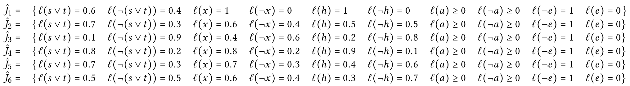
It is well known that for every crisp frame it holds that , see for example [27] for a formal proof. This relationship does not extend to and . We give a counter example. Consider the profile on Table 5. For this profile, and . All the rational judgment sets for , and are given in Table 6. We have that , while
| 0.0 | 0.3 | 0.8 | 0.1 | 0.6 | 0.2 | |
| 0.1 | 0.4 | 0.5 | 0.2 | 0.3 | 0.6 | |
| 0.8 | 0.0 | 0.1 | 0.8 | 0.3 | 0.7 |
| 1 | 1 | 1 | 3.5 | 4.1818 |
| 1 | 0 | 0 | 3.5 | 3.8537 |
| 0 | 1 | 1 | 3.3 | 4.1064 |
| 0 | 1 | 0 | 3.6 | 4.0032 |
The relationship between the distance-based aggregator and the median rule is broken when the distance is used as well and a counter example is not difficult to be found. This is because the relationship between the judgment on and the judgment on is broken - it is not always the case that the likelihood of is a function of the likelihood of .
Lastly we consider a new class of direct aggregators that are not reducible to “classical” JA aggregators.
Most likely prime implicant
One of the oldest and most studied aggregators in “classical” JA is the so called premise-based procedure (PBP) [11]. Some aggregation problems are such that the agenda can be naturally split into two sets: conclusions (or decisions) and premises (or reasons why a decision is taken). For example, the agenda in the example in Table 1 can naturally be split into an agenda of premises and an agenda of conclusions . The PBP aggregator works in two steps: first the majority is calculated for each issue in the premise agenda subset. In the example in Table 1 this would yield the set of premises . Then the constraint is used to entail the judgments on the issues in the conclusion agenda subset. In the example in Table 1 this would yield the collective judgment set . PBP is an aggregator that has many good properties, but it is only applicable to agendas that are split into premises and conclusions. Here we propose a likelihood judgment aggregator that “operates” in the same way as PBP but it is applicable to any agenda.
When the agenda is split into premises and conclusions, the problem is such that the judgments on the premises entail each of the judgments on the conclusions. From a logical perspective, the set of premises is an implicant of the agenda. Let us formally define this concept generalizing it to any agenda.
Definition 3.7.
Given an agenda (not explicitly partitioned into premises and conclusions) and constraints we say that the set is an implicant of if is a consistent (with respect to ) set and either or , for every . is a prime implicant of if is an implicant and there exists no smaller set () that is also an implicant of .
Consider the agenda and constraints of Example 1.1. This agenda has eight prime implicants, i.e., all the consistent three-element subsets of .
We can define a class of irresolute likelihood aggregation functions based on agenda prime implicants and a definition of most likely prime implicant. There are several ways a most likely prime implicant can be defined. We give a few examples. Let be the set of all prime implicants of . Then the most likely prime implicant of is the one with:
-
•
the highest sum of average likelihoods
-
•
the highest minimum average likelihood,
-
•
the highest number of majority supported judgments,
, etc.
Note that the three definitions given above determine three (possibly) different most likely prime implicants for which we could use different names, but for simplicity we omit that.
Once a most likely prime implicant is determined in one of the above described ways, the collective judgment is a union of and the elements of implied by .
Example 3.1.
For the profile, agenda and constraints of Example 1.1, the prime implicant that has the highest sum of average likelihoods is yielding the collective outcome of .
If the agenda and constraints are given in DNF (disjunctive normal form), the prime implicants can be found in polynomial time [39]. To the best of our knowledge, prime implicants have not been used to define aggregation functions in judgment aggregation, with the possible exception of [36] where a distance based function for measuring dissimilarity between two classical judgment sets based on prime implicants has been defined.
4 Properties of aggregators
Having generalized the classical judgment aggregation framework, the immediate question to consider is whether the typical impossibility properties results also hold for aggregators of probabilistic judgments. To establish this, we need to generalize the definitions of aggregation properties. We also need to see whether there are new interesting desirable properties that need to be considered in the new framework. We begin some of this work here.
We begin by exploring the “classical” impossibility theorem [6]. For this we need to define a resolute likelihood aggregator. We then define the properties of universal domain, unanimity, rationality and systematicity.
Definition 4.1.
Let be a probabilistic aggregation frame and let be the set of all rational likelihood profiles for it. A likelihood (resolute) aggregator is a mapping from the set of rational likelihood profiles to the set of consistent and complete crisp judgment sets.
In other words, a (crispifying) aggregator is resolute if it assigns only one collective judgment set to each profile.
Universal domain is the requirement that an aggregator has to be defined for all the probabilistic rational profiles (and all allowable crispifying vectors where applicable). Rationality is the property that produces only consistent and complete crisp judgment sets. These properties are embedded in the Definition 4.1.
An aggregator is dictatorial if there is an information source (a dictator) such that for each likelihood profile , the collective judgment is equal to the collective judgment on the profile , i.e., only the judgment set of the dictator is considered in the aggregation process. Non-dictatorship is the requirement that no information source is a dictator.
In “classical” judgment aggregation, unanimity is the property requiring that if a judgment is in every judgment set in the profile it has to be in the collective judgment set as well. When aggregating likelihood profiles, unanimity has to be defined with respect to some crispifying coefficient , regardless of whether is a direct aggregator or not.
Definition 4.2 (Unanimity).
Let . The aggregator satisfies -unanimity if for every profile of rational probabilistic judgments , , and every it holds that: if : , then .
Lastly we define systematicity. Intuitively, systematicity is satisfied if every two issues that are judged as equally probable in two different profiles are treated equivalently by the aggregation rule .
Definition 4.3 (Systematicity).
Given a profile , let us define to be the projection of on the issue : . The aggregator satisfies systematicity, if for every two profiles and issues , the following holds: implies [ iff ].
The following theorem can easily be proved following the proof method of Theorem 3.7. in [20].
Theorem 4.1.
Consider a frame . Let be the set of all rational likelihood profiles that can be defined for the given frame. The aggregation function satisfies unanimity, rationality and systematicity if and only if is a dictatorial aggregation function.
For other desirable properties that could be applied in our framework we can look to the literature of probabilistic opinion pooling [29, 9] for inspiration.
The systematicity requirement corresponds to a property called Strong setwise function property (SSFP) in opinion pooling [29]. This property requires that the group probability of an event depends only on the individually assigned probabilities of . It was shown that SSFP gives rise to impossibility results in opinion pooling [29]. A weaker property, that is implied by SSFP, is the Zero Preservation Property (ZPP). ZPP is satisfied when for profiles where all of the individually assigned probabilities of an issue are zero, the collective probability of this issue is also zero. The ZPP property is related to the unanimity property in “classical” JA. Here we can define ZPP as -unanimity, namely -unanimity where .
Intuitively, 1-unanimity is desirable: whenever every source is sure that an issue is true (or false), a 1-unanimity satisfying aggregator will capture that certainty. However, unanimity on for does not mean that a rational judgment set such that exists! Recall that we have constraints imposed by the agenda setter on the outcome but not on the judgment sets of the profile. This means that 1-unanimity can only be satisfied in a specific aggregation frame if the set of constraints of the frame allows it. Let us give an example.
Example 4.1.
Let be a probabilistic aggregation frame such that and . Let be a consistent probabilistic profile in this frame such that and are in every individual judgment set in . Then 1-unanimity requires that for every but none such is in .
As seen in the above example, whether an aggregation function can satisfy 1-unanimity is a property of the aggregation frame. We can define the ZPP property for likelihood aggregators (the definition also extends to irresolute direct and indirect aggregators as well) as 1-unanimity when the constraints allow it.
Definition 4.4 (Zero preservation property).
Let be a probabilistic aggregation frame. Given a profile , we define the set as
Namely, the set contains all the agenda issues that have been unanimously awarded likelihood 1 in . We say that an aggregator satisfies the zero preservation property if for all it holds that if is consistent with , then .
We consider one more intuitive property of probabilistic aggregators, that of convexity [29]. Convexity states that the collectively assigned (minimal) probability on an issue should be a value no smaller than the smallest and no higher than the highest individually assigned probability on that issue. For the direct aggregators this property is not applicable, but it is so for the crispifying ones.
Definition 4.5 (Convexity).
Let be one of the probabilistic judgment sets assigned to profile by a function (before crispification). For a given , let and . We say that satisfies convexity when for all collective and every , if then .
It can directly be observed that satisfies convexity and that satisfies ZPP and universal domain. However does not satisfy rationality because the sets in are not always rational sets of judgments.
The aggregator satisfies universal domain and non-dictatorship by design. It is clear that also satisfies ZPP.
The distance-based direct aggregators satisfy universal domain and non-dictatorship by design, however it is safe to conjecture that they will not satisfy ZPP for the same reason that distance-based classical aggregators do not satisfy unanimity [32] – for an agenda with sufficiently many issues, a judgment set that does not contain the unanimously likely judgment might end up being “closer” to the profile.
With the most likely prime implicant class of aggregators, universal domain and rationality will be satisfied by design. However, ZPP will not be satisfied - when the unanimously supported issue is not in the prime implicant its inclusion in the collective judgment set will not be guaranteed.
5 Related work
As mentioned in the introduction, the area of probabilistic opinion pooling is concerned with aggregating probability functions into a single one. As opposed to standard probabilistic opinion pooling, our logic-based approach:
-
1.
allows for an arbitrary agenda, namely instead of taking the entire -algebra, the agenda can be limited to the important issues of consideration in the actual context;
-
2.
We do not limit ourselves to expressing point probabilities over the issues (but we do include that option as well);
-
3.
The result of the opinion aggregation is a set of propositional statements, hence a final decision, and not a probabilistic consensus.
Dietrich and List [9] generalize opinion pooling to general agendas and examine properties and impossibility results. However, their work does not define any particular aggregators and also 2) and 3) are not the case there.
The problem of transforming degrees of belief into binary beliefs is known as belief-binarization. Dietrich and List [10] study how a profile of Boolean judgments, that has been transformed into a vector of beliefs (for example a profile from Table 1 becomes the vector ) can be “binarized” into a consistent set of Boolean judgments. In [10], however, only binary profiles are aggregated.
There are several approaches towards aggregating imprecise probabilities (IP), like aggregation of probability intervals in [30], subjective opinion fusion in [23], etc. More recently [38] extended pooling properties to IPs using convex functions. Moreover, they go further and aggregate precise probabilities into imprecise (the convex hull of the input probabilities as a proof of concept) arguing that IP models are better suited as models of rational consensus. Allowing for inequalities in the likelihood judgments, we allow for modeling IP in the individual judgments. However, unlike [38] we require the collective judgment to be crisp since our goal is to define specific aggregators that support the decision making in various contexts.
Dietrich and List [6] generalize classical JA assuming formulas from a general logic and prove impossibility theorems. They show that the model is applicable to, for example, propositional, modal, and many-valued logic. The model is not directly applicable to the likelihood logic we use here, since it assumes that the agenda issues are formulas in the particular logic. Since it does not make sense to choose a finite agenda of likelihood formulas, we express the issues in propositional logic and use likelihood formulas for the judgments. The latter makes our framework fit better in the general theory of aggregation of propositional attitudes in [8], that integrates probabilistic opinion pooling and judgment aggregation. In this theory, profiles consist of attitude functions (which can be probability functions, truth-value functions, etc.) defined over finite subset of a -algebra (an agenda). We believe that defining notions on the level of a syntax has certain advantages, explicitly defining the concept of rationality being one of them.
It is not always possible to have complete information, sometimes some sources will not be able to provide information on all of the issues. Although impossibility results involving abstentions have been shown [12], designing functions to aggregate the so called incomplete judgments is not given a lot of attention in the JA literature [40, 35]. By showing how crisp profiles can be represented as likelihood ones and designing likelihood judgment aggregators, we enable probabilistic judgment aggregation to also be used for aggregating crisp incomplete judgment sets in a straightforward way.
Interpreting the likelihood operator with a possibility measure leads to the formula being equivalent to the formula as well as the (uniform) crispifying being equivalent to -cut in possibility theory. There are various methods of information fusion considered in this theory [13]. However, they focus on merging information about the true state of a variable or a proposition and take a set theoretic approach to defining the merging functions while we, on the other hand, follow the tradition of judgment aggregation and social-choice theory and take an agenda of (logically related) issues as a starting point. This means that both the (choice of) definitions of the aggregators, and the choice of crispifying coefficients depend on the agenda. Moreover, our goal is not just to merge the imprecise information coming from the different sources, but to make a decision about the true state of the agenda issues.
Probabilistic belief merging is considered in [33, 34]. In belief merging sets of formulas, possibly likelihood formulas, are called knowledge bases. Knowledge bases from several sources, that can be mutually inconsistent, are merged to obtain a consistent knowledge base. The difference between belief merging and judgment aggregation has been analyzed in [18]. Essentially, in belief merging the knowledge bases do not share the same agenda, which entails different properties to be desired for the merging operators as compared to the desired properties for judgment aggregation functions.
6 Conclusions and future work
We consider as the main contribution of our paper the definition of various functions for aggregating likelihood judgments on logically related issues. Furthermore, we show how these aggregators relate to classical judgment aggregation function, and in turn, through the results shown in [24] and [14], how likelihood judgment aggregation relates to voting methods. We also define desirable properties for the aggregation functions and show that the classical impossibility results hold here as well.
Some more consideration needs to be given to further distinguish the likelihood profile aggregators. From the examples we can observe that very different outcomes are produced for the same profile by different aggregators. The minimal set of properties we discuss is not sufficient to allow a user to choose which is the best aggregator for a given probabilistic frame. In light of new properties, particularly the direct aggregators need to be carefully studied.
More properties from opinion pooling can be considered and “translated” into our extended JA framework. An interesting candidate is the so called Independence Preservation (IP) property which intuitively requires that if two issues are probabilistically independent according to all information sources, then this independence should be preserved in the collectively assigned probabilities for the two issues. This has been explored by Wagner in [41] for the case of aggregating point probabilities over an agenda of mutually exclusive events; [38] explores the imprecise probabilities case. Note that to represent probabilistic independencies in the judgments, we need to either extend the logic of likelihood with polynomial likelihood formulas or include likelihood independence formulas as defined in [22] directly in the language. Then we could define IP properties alike [41] and [38] and see what are the consequencies of their impossibility results in our platform. We notice also that the IP property is reminiscent of the agenda separability property studied in [26]. One direction of future work is to establish this intuitive connection and explore other such connections between probability aggregation properties and JA properties.
We believe that with this work we have made several contributions to the classical JA theory as well: We have significantly extended the classical binary judgment aggregation framework, opening up this social choice method for applications in new AI domains, particularly involving the aggregation of uncertain judgments; our framework allows for not only uncertainties but also abstentions to be modelled using , which is a neglected feature in judgment aggregation frameworks overall; furthermore, we generalize the assumption that the same relations between issues should hold for both the information sources and the aggregated result. This “double constraint” framework is actually very intuitive [14].
Having a probabilistic framework also opens possibilities to study the truth-tracking properties of judgment aggregators, namely how good is a function in aggregating profiles into the most likely judgments. This area of judgment aggregation is still relatively little explored [4]. We intend to explore truth-tracking in future work.
We believe that there is a possibility for applying our work to prediction markets [42], specifically in extending the agenda of predictions (which is typically consisting of states of a random variable) to a set of logically related statements. Prediction markets [2] are forums for trading contracts for outcomes of future events. Each market participant possesses certain information about the event in question, and conveys this information to the market by the way she trades contracts. The contract price is a result of aggregation of the information possessed by all the participants, hence is an estimator of the probability of the event in question. We believe we could seek for inspiration in defining new aggregators under our platform by studying the methods of information fusion that various prediction markets apply.
References
- [1]
- [2] A. Barbu & N. Lay (2012): An Introduction to Artificial Prediction Markets for Classification. Journal of Machine Learning Research 13, pp. 2177–2204. Available at http://dl.acm.org/citation.cfm?id=2503312.
- [3] G. Boella, G. Pigozzi, M. Slavkovik & L. van der Torre (2011): Group Intention Is Social Choice with Commitment. In M. De Vos, N. Fornara, J. Pitt & G. Vouros, editors: COIN in Agent Systems VI, LNCS 6541, Springer, Germany, pp. 152–171, 10.1007/978-3-642-21268-09.
- [4] I. Bozbay (2019): Truth-tracking Judgment Aggregation over Interconnected Issues. Social Choice and Welfare, pp. 1–34, 10.1007/s00355-019-01186-6.
- [5] M.M. Deza & E. Deza (2009): Encyclopedia of Distances. Springer, Germany, 10.1007/978-3-642-00234-2.
- [6] F. Dietrich (2007): A Generalized Model of Judgment Aggregation. Social Choice and Welfare 28(4), pp. 529–565, 10.1007/s00355-006-0187-y.
- [7] F. Dietrich (2014): Scoring Rules for Judgment Aggregation. Social Choice and Welfare 42(4), pp. 873–911, 10.1007/s00355-013-0757-8.
- [8] F. Dietrich & C. List (2010): The Aggregation of Propositional Attitudes: Towards a General Theory. Oxford Studies in Epistemology 3, pp. 215–234. Available at http://eprints.lse.ac.uk/id/eprint/31600.
- [9] F. Dietrich & C. List (2017): Probabilistic Opinion Pooling Generalized. Part one: General Agendas. Social Choice and Welfare 48(4), pp. 747–786, 10.1007/s00355-017-1034-z.
- [10] F. Dietrich & C. List (2018): From Degrees of Belief to Binary Beliefs: Lessons from Judgment-aggregation Theory. The Journal of Philosophy 115, pp. 225–270, 10.5840/jphil2018115516.
- [11] F. Dietrich & P. Mongin (2010): The Premisse-Based Approach to Judgment Aggregation. Journal of Economic Theory 145(2), pp. 562–582, 10.1016/j.jet.2010.01.011.
- [12] E. Dokow & R. Holzman (2010): Aggregation of Binary Evaluations with Abstentions. Journal of Economic Theory 145(2), pp. 544 – 561, 10.1016/j.jet.2009.10.015.
- [13] D. Dubois & H. Prade (2001): Possibility Theory in Information Fusion. In G. Della Riccia, H.J. Lenz & R. Kruse, editors: Data Fusion and Perception, Springer Vienna, Vienna, pp. 53–76, 10.1007/978-3-7091-2580-93.
- [14] U. Endriss (2018): Judgment Aggregation with Rationality and Feasibility Constraints. In: Proceedings of the 17th International Conference on Autonomous Agents and MultiAgent Systems, AAMAS ’18, International Foundation for Autonomous Agents and Multiagent Systems, Richland, SC, pp. 946–954. Available at http://dl.acm.org/citation.cfm?id=3237383.3237840.
- [15] U. Endriss, U. Grandi, R. de Haan & J. Lang (2016): Succinctness of Languages for Judgment Aggregation. In: Proceedings of KR-2016, AAAI Press, USA, pp. 176–186. Available at http://www.aaai.org/ocs/index.php/KR/KR16/paper/view/12851.
- [16] U. Endriss & R. de Haan (2015): Complexity of the Winner Determination Problem in Judgment Aggregation: Kemeny, Slater, Tideman, Young. In: Proceedings of the 2015 International Conference on Autonomous Agents and Multiagent Systems, AAMAS ’15, International Foundation for Autonomous Agents and Multiagent Systems, Richland, SC, pp. 117–125. Available at http://dl.acm.org/citation.cfm?id=2772879.2772897.
- [17] P. Everaere, S. Konieczny & P. Marquis (2014): Counting votes for aggregating judgments. In: International conference on Autonomous Agents and Multi-Agent Systems, AAMAS ’14, Paris, France, May 5-9, 2014, pp. 1177–1184. Available at http://dl.acm.org/citation.cfm?id=2617436.
- [18] P. Everaere, S. Konieczny & P. Marquis (2015): Belief Merging versus Judgment Aggregation. In: Proceedings of the AAMAS-2015, pp. 999–1007. Available at http://dl.acm.org/citation.cfm?id=2773279.
- [19] R. Fagin, J. Y. Halpern & N. Megiddo (1990): A Logic for Reasoning about Probabilities. Information and Computation 87, pp. 78–128, 10.1016/0890-5401(90)90060-U.
- [20] D. Grossi & G. Pigozzi (2014): Judgment Aggregation: A Primer. Morgan and Claypool Publishers, San Rafael, CA, USA, 10.2200/S00559ED1V01Y201312AIM027.
- [21] J. Y. Halpern (2005): Reasoning about uncertainty. MIT Press. Available at https://mitpress.mit.edu/books/reasoning-about-uncertainty-second-edition.
- [22] M. Ivanovska & M. Giese (2010): Probabilistic Logic with Conditional Independence Formulae. In: Proceedings of ECAI 2010 - 19th European Conference on Artificial Intelligence, pp. 983–984, 10.3233/978-1-60750-606-5-983.
- [23] A. Jøsang (2016): Subjective Logic: A Formalism for Reasoning Under Uncertainty. Artificial Intelligence: Foundations, Theory, and Algorithms, Springer International Publishing, 10.1007/978-3-319-42337-1.
- [24] J. Lang & M. Slavkovik (2013): Judgment Aggregation Rules and Voting Rules. In: Proceedings of the 3rd International Conference on Algorithmic Decision Theory, Lecture Notes in Artificial Intelligence 8176, Springer-Verlag, Germany, pp. 230–244, 10.1007/978-3-642-41575-318.
- [25] J. Lang & M. Slavkovik (2014): How Hard is it to Compute Majority-Preserving Judgment Aggregation Rules? In: Proceedings of ECAI-2014, Frontiers in Artificial Intelligence and Applications 263:ECAI 2014, IOS Press, Netherlands, pp. 501–506, 10.3233/978-1-61499-419-0-501.
- [26] J. Lang, M. Slavkovik & S. Vesic (2016): Agenda Separability in Judgment Aggregation. In: Proceedings of the 30th AAAI Conference on Artificial Intelligence (AAAI-16), pp. 1016–1022. Available at http://www.aaai.org/ocs/index.php/AAAI/AAAI16/paper/view/12084.
- [27] L. Lang, P. Pigozzi, M. Slavkovik, L. van der Torre & S. Vesic (2016): A partial taxonomy of judgment aggregation rules, and their properties. Social Choice and Welfare 48, pp. 1–30, 10.1007/s00355-016-1006-8.
- [28] C. List & C. Puppe (2009): Judgment aggregation: A survey. In P. Anand, C. Puppe & P. Pattanaik, editors: The Handbook of Rational and Social Choice, Oxford University Press, UK, 10.1093/acprof:oso/9780199290420.003.0020.
- [29] C. Martini & J Sprenger (2017): Opinion Aggregation and Individual Expertise. In: Scientific Collaboration and Collective Knowledge: New Essays, Oxford Scholarship, UK, 10.1093/oso/9780190680534.001.0001.
- [30] S. Moral & J. Del Sagrado (1998): Aggregation of Imprecise Probabilities. In: Aggregation and fusion of imperfect information, Springer, Germany, pp. 162–188, 10.1007/978-3-7908-1889-510.
- [31] K. Nehring & M. Pivato (2013): Majority Rule in the Absence of a Majority. MPRA Paper 46721, University Library of Munich, Germany, 10.1016/j.jet.2019.05.006.
- [32] G. Pigozzi, M. Slavkovik & L. van der Torre (2009): A Complete Conclusion-Based Procedure for Judgment Aggregation. In F. Rossi & A. Tsoukias, editors: Algorithmic Decision Theory, Lecture Notes in Computer Science 5783, Springer, Berlin Heidelberg, pp. 1–13, 10.1007/978-3-642-04428-11.
- [33] N. Potyka, E. Acar, M. Thimm & H. Stuckenschmidt (2016): Group Decision Making via Probabilistic Belief Merging. In: Proceedings of the Twenty-Fifth International Joint Conference on Artificial Intelligence, IJCAI’16, AAAI Press, pp. 3623–3629. Available at http://dl.acm.org/citation.cfm?id=3061053.3061126.
- [34] N. Potyka & M. Thimm (2017): Inconsistency-tolerant Reasoning over Linear Probabilistic Knowledge Bases. International Journal of Approximate Reasoning 88, pp. 209 – 236, 10.1016/j.ijar.2017.06.002.
- [35] M. Slavkovik (2012): Judgment Aggregation for Multiagent Systems. Doctoral Thesis, University of Luxembourg, Uitgeverij BOXPress, Netherlands. Available at http://icr.uni.lu/Marija/thesis.pdf.
- [36] M. Slavkovik & T. Ågotnes (2014): Measuring Dissimilarity between Judgment Sets. In: Logics in Artificial Intelligence, Lecture Notes in Computer Science 8761, Springer International Publishing, pp. 609–617, 10.1007/978-3-319-11558-044.
- [37] M. Slavkovik & G. Boella (2012): Recognition-primed group decisions via judgement aggregation. Synthese 189(1), pp. 51–65, 10.1007/s11229-012-0161-4.
- [38] R. T. Stewart & I. O. Quintana (2018): Probabilistic Opinion Pooling with Imprecise Probabilities. Journal of Philosophical Logic 47(1), pp. 17–45, 10.1007/s10992-016-9415-9.
- [39] T. Strzemecki (1992): Polynomial-time Algorithms for Generation of Prime Implicants. Journal of Complexity 8(1), pp. 37 – 63, 10.1016/0885-064X(92)90033-8.
- [40] Z. Terzopoulou, U. Endriss & R. de Haan (2018): Aggregating Incomplete Judgments: Axiomatisations for Scoring Rules. In: Proceedings of the COMSOC-2018, online. Available at http://research.illc.uva.nl/COMSOC/proceedings/comsoc-2018/TerzopoulouEtAlCOMSOC2018.pdf.
- [41] C. Wagner (1984): Aggregating Subjective Probabilities: Some Limitative Theorems. Notre Dame Journal of Formal Logic 25, pp. 233–240, 10.1305/ndjfl/1093870630.
- [42] J. Wolfers & E. Zitzevitz (2004): Prediction Markets. Journal of Economic Perspectives 18(2), pp. 107–126, 10.1257/0895330041371321.