Strategic Voting Under Uncertainty About the Voting Method

Abstract

Much of the theoretical work on strategic voting makes strong assumptions about what voters know about the voting situation. A strategizing voter is typically assumed to know how other voters will vote and to know the rules of the voting method. A growing body of literature explores strategic voting when there is uncertainty about how others will vote. In this paper, we study strategic voting when there is uncertainty about the voting method. We introduce three notions of manipulability for a set of voting methods: sure, safe, and expected manipulability. With the help of a computer program, we identify voting scenarios in which uncertainty about the voting method may reduce or even eliminate a voter’s incentive to misrepresent her preferences. Thus, it may be in the interest of an election designer who wishes to reduce strategic voting to leave voters uncertain about which of several reasonable voting methods will be used to determine the winners of an election.

1 Introduction

A well-known fact in the study of voting methods is that strategic voting cannot be avoided (see, e.g., [36, 22]). A voter has an incentive to vote strategically, or manipulate, if she will achieve a preferable outcome by misrepresenting her true preferences about the candidates. There are two fundamental results showing that every reasonable voting method is susceptible to strategic voting. The Gibbard-Satterthwaite theorem [14, 33] shows that every voting method for three or more candidates that is resolute (i.e., always elects a single winner), unanimous (i.e., never elects a candidate $y$ if all voters rank another candidate $x$ above $y$), and non-dictatorial (i.e., does not always elect the favorite candidate of some distinguished voter) can be manipulated. To study strategizing for irresolute voting methods, which may select more than one candidate as a winner, additional assumptions are needed about the voters’ rankings of sets of candidates. The Duggan-Schwartz theorem [10] shows that every voting method—whether resolute or irresolute—for three or more candidates that is non-imposed (i.e., any candidate can be elected) and has no nominator (i.e., no voter can always ensure that her top ranked candidate is among the set of winners) can be manipulated by a optimist or pessimist, defined as a voter who compares sets of candidates in terms of her highest (resp. lowest) ranked candidate in each set. Related results by Kelly [20], Benoit [3], Feldman [12], and Gärdenfors [13], among others, show that manipulation is unavoidable under different assumptions about how to lift a voter’s ranking of candidates to sets of candidates.

In the theorems mentioned above, a voter’s decision to manipulate relies on strong assumptions about what the voter knows about the voting situation. Two key assumptions are: (1) the strategizing voter knows how the other voters in the population will vote or have voted; (2) the strategizing voter knows and understands the rules of the voting method. There is a growing body of literature that explores weakening assumption (1) [7, 28, 6, 23, 31, 37]. One reason voters may be uncertain about how other voters will vote, even if they know other voters’ true preferences, is because they think that other voters might be voting strategically. There are sophisticated game-theoretic models that explore the implications of weakening assumption (1) for this reason (consult part II of [22] for an overview of this literature). Whatever the reason, when voters have partial information about how other voters will vote, the decision about whether to manipulate is more complicated, since voters are uncertain about which sets of winners will result from their decision to manipulate. One natural assumption is that voters are risk averse and only strategize when doing so cannot lead to a worse outcome (according to their true preferences) and might lead to a better outcome [7] (cf. [31] for other assumptions about how voters decide to strategize).

The potentially negative aspects of strategic voting (see, e.g., [32, 8]) have motivated the search for barriers against manipulation. One potential barrier, investigated mostly in the AI literature, is the computational complexity of determining a profitable manipulation for a given voting method (see, e.g., [11, 8]). In this paper, we will investigate another potential barrier against strategic voting: adding uncertainty about the voting method that will be used to determine the set of winners. Thus, we weaken assumption (2) above. Suppose that $S$ is a set of voting methods. We assume that the voters know that one of the methods from $S$ will be used to select the winners, but they do not know which one—hence we call $S$ the uncertainty set. To simplify the initial study, in this paper we assume that a strategizing voter knows how the other voters will vote or have voted. This assumption is not unrealistic in certain voting situations; for example, in a hiring committee meeting in which committee members are asked to sequentially report their rankings of job candidates, the committee member last in the sequence will already know how all the other members have ranked the candidates.

As in the situation where a voter has partial information about how other voters will vote, in the situation where a voter has uncertainty about the voting method, the voter must take into account different possible winning sets of candidates when deciding whether to strategize. Given a ranking of sets of candidates, we consider three ways for a voter to solve this decision problem. From the most conservative to the least conservative, the three types of manipulation are:

1. Sure manipulation: It is certain that submitting an insincere ranking will lead to a better outcome no matter which voting method is used.

2. Safe manipulation: It is certain that submitting an insincere ranking will lead to an outcome that is at least as good and might lead to a better outcome.

3. Expected manipulation: Given a probability distribution on the set of voting methods, submitting an insincere ranking is more likely to lead to a better outcome than to lead to a worse outcome.

We aim to find combinations of voting methods that reduce or even eliminate a voter’s incentive to strategize (given one of the above notions of manipulation and a ranking of sets of candidates). That is, does uncertainty about the voting method reduce the chance that voters will strategize?

If so, it may be in the interest of an election designer who wishes to reduce strategic voting to leave voters uncertain about which of several voting methods will be used to determine the winners of an election. Though perhaps implausible in the case of a democratic political election, creating such uncertainty does not seem an implausible choice by, e.g., the Chair of a hiring committee. Moreover, if committee members judge each of the possible voting methods to be reasonable and also wish to reduce strategic voting, they may well endorse the choice of the Chair to create such uncertainty.

Another way that voters may be uncertain about the outcome of an election is that a voting method may use randomization to select the winners. A probabilistic voting method assigns a lottery over the set of candidates to each collection of rankings of the candidates for the voters (see [5] for a recent survey of results about probabilistic voting methods). Gibbard [15] noted that a random dictatorship is immune to strategizing. Suppose that $S$ is a set of dictatorships—one for each voter. After the voters submit their rankings, one of the dictatorships in $S$ is chosen, and the candidate ranked first by the dictator is selected as the winner. Assuming voters submit rankings of the candidates without ties, this method always selects a single winner. It is clear that no voter has an incentive to misrepresent their top choice, since either they will not be chosen as the dictator, in which case their ranking will be ignored, or they will be chosen as the dictator, in which case their top choice is guaranteed to win. Of course, each dictatorship is immune to strategizing by itself. Beyond this example of random dictatorship, there are general results suggesting that randomization can be an effective barrier to manipulation [27, 2].

The relationship between our work and probabilistic voting methods is clarified at the end of this paper. In short, although any uncertainty set $S$ of voting methods determines a probabilistic voting method $F_{\_}S$, none of our three notions of manipulation above with respect to $S$ is equivalent to a standard notion of manipulation with respect to the probabilistic voting method $F_{\_}S$. In addition, since the mapping $S\mapsto F_{\_}S$ from uncertainty sets of voting methods to probabilistic voting methods is not one-to-one, there is no obvious definition of sure, safe, or even expected manipulation for probabilistic voting methods such that for any uncertainty set $S$ of voting methods, $S$ is susceptible to sure/safe/expected manipulation if and only if $F_{\_}S$ is susceptible to sure/safe/expected manipulation. Thus, there is no obvious way to reframe our investigation purely in the language of probabilistic voting methods.

Both our approach and that of probabilistic voting methods involve a loss of transparency at the time of the vote. However, the approaches seem to differ in the explainability of the outcome after the vote. In our approach, the election designer may simply inform voters after the vote of which voting method $f$ from $S$ was used to determine the outcome of the election, so the algorithm for $f$ can be used to explain why the election had one outcome rather than another. This may be a more intelligible reason for voters than “this was the outcome of the lottery.” Abstractly, the difference is that in our setting, initially the voters have subjective uncertainty about which deterministic mechanism will be used; but after this subjective uncertainty is removed, there is an explanation of why the election had one outcome rather than another in terms of the deterministic mechanism applied to the voters’ inputs. By contrast, with a probabilistic voting method, the only available “explanation” of the outcome is in terms of an inherently stochastic mechanism applied to the voters’ inputs, which may fail to explain why the election had one outcome rather than another with non-zero probability (cf. [19, p. 24], [30, p. 238]). Of course, whether such a contrastive explanation is desirable may vary from case to case.

Our findings in this paper are of two main types: analytic results with mathematical proofs and data from computer searches. For these searches we generalize to sets of voting methods a standard index of manipulability for a single voting method, known as the Nitzan-Kelly index [26, 21], which gives the percentage of profiles with $n$ candidates and $m$ voters in which at least one voter in the profile has an incentive to manipulate. In probabilistic terms, assuming the Impartial Culture Model [16] in which every profile is equally probable, this index gives the probability that in a randomly chosen profile, at least one voter has an incentive to manipulate. Similarly, we report data on the percentage of profiles in which at least one voter has an incentive to manipulate against a set $S$ of voting methods. All of the data in the paper were produced by a Python script available at https://github.com/epacuit/strategic-voting.

The rest of the paper is organized as follows. The next section introduces our formal framework, including the definitions of the voting methods we study in this paper. The three notions of manipulation are studied in Sections 3, 4, and 5, respectively. Section 6 discusses the connections with probabilistic social choice. Finally, in Section 7 we conclude with some pointers to future work.

2 Preliminaries

Let $C$ be a nonempty finite set of candidates and $V$ a nonempty finite set of voters. We use lower case letters from the beginning and end of the alphabet $a,b,c,\ldots,x,y,z,\ldots$ for elements of $C$ and lower case letters from the middle of the alphabet $i,j,k,\ldots$ for elements of $V$.

A voter’s ranking of the set of candidates is a strict linear order $P$ on $C$. Let $L(C)$ be the set of all strict linear orders on $C$. For $P\in L(C)$ and $X\subseteq C$, let $\mathrm{max}(X,P)$ be the maximally ranked element of $X$, i.e., $\mathrm{max}(X,P)=y$ where for all $x\in X$, if $x\neq y$, then $y\mathrel{P}x$ (such an element always exists since $P$ is assumed to be a strict linear order). Similarly, let $\mathrm{min}(X,P)$ be the minimally ranked element of $X$, i.e., $\mathrm{min}(X,P)=y$ where for all $x\in X$, if $x\neq y$, then $x\mathrel{P}y$. We say $y\in C$ is ranked $r$th by $P$ when $|\{x\in C\ |\ x\mathrel{P}y\}|=r-1$. So, for example, $y$ is ranked 1st by $P$ if and only if $\mathrm{max}(C,P)=y$. To simplify our notation, we specify a ranking by simply listing candidates from highest to lowest in the ranking, e.g., $a\,b\,c\,d$ for the ranking $a\mathrel{P}b\mathrel{P}c\mathrel{P}d$.

A profile $\mathbf{P}$ for $(C,V)$ is an element of $L(C)^{V}$, i.e., a function assigning to each $i\in V$ a relation $\mathbf{P}_{\_}i\in L(C)$. If $|C|=n$ and $|V|=m$, we call a profile for $(C,V)$ an $(n,m)$-profile. A pointed profile for $(C,V)$ is a pair $(\mathbf{P},i)$ where $\mathbf{P}$ is a profile and $i\in V$. For $x,y\in C$, let $\mathbf{P}(x,y)=\{i\in V\mid x\mathbf{P}_{\_}iy\}$. We write $\mathbf{N}_{\_}\mathbf{P}(x,y)$ for the number of voters in $\mathbf{P}$ ranking $x$ above $y$, i.e., $\mathbf{N}_{\_}\mathbf{P}(x,y)=|\mathbf{P}(x,y)|$. We say that a majority prefers $x$ to $y$ in $\mathbf{P}$, denoted $x>^{M}_{\_}\mathbf{P}y$, when $\mathbf{N}_{\_}\mathbf{P}(x,y)>\mathbf{N}_{\_}\mathbf{P}(y,x)$. Let $Net_{\_}\mathbf{P}(x,y)=\mathbf{N}_{\_}{\mathbf{P}}(x,y)-\mathbf{N}_{\_}{\mathbf{P}}(y,x)$. So $x>_{\_}\mathbf{P}^{M}y$ if and only if $Net_{\_}\mathbf{P}(x,y)>0$. Finally, from the strict linear order $\mathbf{P}_{\_}i$ we define the weak relation $\mathbf{R}_{\_}i$ by $x\mathbf{R}_{\_}iy$ iff $x\mathbf{P}_{\_}iy$ or $x=y$.

A voting method for $(C,V)$ is a function assigning a nonempty subset of candidates, called the winning set, to each profile, i.e., $f:L(C)^{V}\rightarrow\wp(C)\setminus\{\varnothing\}$. The following are the voting methods we will discuss in this paper (also see, e.g., [29]).

(1) Positional scoring rules: Suppose $\langle s_{\_}1,s_{\_}2,\ldots,s_{\_}m\rangle$ is a vector of numbers, called a scoring vector, where for each $l=1,\ldots,m-1$, $s_{\_}l\geq s_{\_}{l+1}$. Suppose ${P}\in L(C)$. The score of $x\in C$ given $P$ is $score(P,x)=s_{\_}r$ where $r$ is the rank of $x$ in $P$. For each profile $\mathbf{P}$ and $x\in C$, let $score(\mathbf{P},x)=\sum_{\_}{i=1}^{n}score(\mathbf{P}_{\_}i,x)$. A positional scoring rule for a scoring vector $\vec{s}$ assigns to each profile $\mathbf{P}$ the set of candidates that maximize their score according to $\vec{s}$ in $\mathbf{P}$. That is, a voting method $f$ is a positional scoring rule for a scoring vector $\vec{s}$ provided that for all $\mathbf{P}\in L(C)^{V}$, $f(\mathbf{P})=\mathrm{argmax}_{\_}{x\in C}score(\mathbf{P},x)$. We study two such rules:

$\mathtt{Borda}$: the positional scoring rule for ${\langle n-1,n-2,\ldots,1,0\rangle}$.

$\mathtt{Plurality}$: the positional scoring rule for $\langle 1,0,\ldots,0\rangle$.

(2) The Condorcet winner in a profile $\mathbf{P}$ is a candidate $x\in C$ that is the maximum of the majority ordering, i.e., for all $y\in C$, if $x\neq y$, then $x>_{\_}\mathbf{P}^{M}y$. The Condorcet voting method is:

$\mathtt{Condorcet}(\mathbf{P})=\begin{cases}\{x\}&\text{if $x$ is the Condorcet winner in $\mathbf{P}$}\\ C&\text{if there is no Condorcet winner}.\end{cases}$

(3) The win-loss record for a candidate $x\in C$ in a profile $\mathbf{P}$ is the number of candidates $z$ such that a majority prefers $x$ to $z$ in $\mathbf{P}$ minus the number of candidates $z$ such that a majority prefers $z$ to $x$ in $\mathbf{P}$. Formally, for each $\mathbf{P}$ and $x\in C$, let $wl_{\_}\mathbf{P}(x)=|\{z\ |\ Net_{\_}\mathbf{P}(x,z)>0\}|-|\{z\ |\ Net_{\_}\mathbf{P}(z,x)>0\}|$. The Copeland winners are the candidates with maximal win-loss records: $\mathtt{Copeland}(\mathbf{P})=\mathrm{argmax}_{\_}{x\in C}(wl_{\_}\mathbf{P}(x))$.

(4) The support for a candidate $x\in C$ in a profile $\mathbf{P}$ is found by calculating for each candidate $y\neq x$ the number of voters who rank $x$ above $y$ and then taking the minimum of these values. Formally, for each $\mathbf{P}$ and $x\in C$, let $supp(x,\mathbf{P})=\mathrm{min}(\{\mathbf{N}_{\_}\mathbf{P}(x,y)\ |\ y\in C,y\neq x\})$. The MaxMin (also known as Simpson’s Rule) winners are the candidates with maximal support: $\texttt{MaxMin}(\mathbf{P})=\mathrm{argmax}_{\_}{x\in C}(supp(x,\mathbf{P}))$.

(5) PluralityWRunoff: Calculate the plurality score for each candidate—the number of voters who rank the candidate first. If there are 2 or more candidates with the highest plurality score, remove all other candidates and select the Plurality winners from the remaining candidates. If there is one candidate with the highest plurality score, remove all candidates except the candidates with the highest or second-highest plurality score, and select the Plurality winners from the remaining candidates.

(6) Hare: Iteratively remove all candidates with the fewest number of voters who rank them first, until there is a candidate who is a majority winner, i.e., ranked first by a majority of voters. If, at some stage of the removal process, all remaining candidates have the same number of voters who rank them first (so all candidates would be removed), then all remaining candidates are selected as winners.

(7) Coombs: Iteratively remove all candidates with the most number of voters who rank them last, until there is a candidate who is a majority winner. If, at some stage of the removal process, all remaining candidates have the same number voters who rank them last (so all candidates would be removed), then all remaining candidates are selected as winners.

(8) Baldwin: Iteratively remove all candidates with the smallest Borda score, until there is a single candidate remaining. If, at some stage of the removal process, all remaining candidates have the same Borda score (so all candidates would be removed), then all remaining candidates are selected as winners.

(9) Rather than removing candidates with the lowest Borda score, the next two methods remove all candidates who have a Borda score below the average Borda score for all candidates. There are two versions of this voting method [25]: StrictNanson iteratively removes all candidates whose Borda score is strictly smaller than the average Borda score (of the candidates remaining at that stage), until one candidate remains. WeakNanson iteratively removes all candidates whose Borda score is less than or equal to the average Borda score (of the candidates remaining at that stage), until one candidate remains. If, at some stage of the removal process, all remaining candidates have the same Borda score (so all candidates would be removed), then all remaining candidates are selected as winners.

Definition 2.1.

Let $\mathsf{Methods}$ be the set of 11 voting methods described above.

We are interested in situations in which the strategizing voter is uncertain about which voting method will be used to determine the winner(s). As noted in Section 1, we represent such uncertainty by a set $S$ of voting methods, called the uncertainty set. This is the set of voting methods $f$ such that it is consistent with the strategizing voter’s knowledge that $f$ will be used.

Each of the above methods may select more than one winner for a given profile. Thus, to discuss strategizing, one needs a notion of when one set of candidates is “preferable” to another for a particular voter. The following are the standard notions from the literature on strategic voting (see, e.g., [36]).

Definition 2.2.

Let $\mathbf{P}$ be a profile, $i\in V$, and $X,Y\subseteq C$. We define the following dominance notions, each of which has a nonstrict ($\geq$) and strict ($>$) version:
weak: (a) $X\geq_{\_}{\mathbf{P}_{\_}i}^{weak}Y$ iff $\forall x\in X$ $\forall y\in Y$: $x\mathbf{R}_{\_}iy$;  (b) $X>_{\_}{\mathbf{P}_{\_}i}^{weak}Y$ iff $X\geq_{\_}{\mathbf{P}_{\_}i}^{weak}Y$ and $\exists x\in X$ $\exists y\in Y$: $x\mathbf{P}_{\_}iy$.

optimistic: (a) $X\geq_{\_}{\mathbf{P}_{\_}i}^{Opt}Y$ iff $\mathrm{max}(X,\mathbf{P}_{\_}i)\mathrel{\mathbf{R}_{\_}i}\mathrm{max}(Y,\mathbf{P}_{\_}i)$; (b) $X>_{\_}{\mathbf{P}_{\_}i}^{Opt}Y$ iff $\mathrm{max}(X,\mathbf{P}_{\_}i)\mathrel{\mathbf{P}_{\_}i}\mathrm{max}(Y,\mathbf{P}_{\_}i)$.

pessimistic: (a) $X\geq_{\_}{\mathbf{P}_{\_}i}^{Pes}Y$ iff $\mathrm{min}(X,\mathbf{P}_{\_}i)\mathrel{\mathbf{R}_{\_}i}\mathrm{min}(Y,\mathbf{P}_{\_}i)$; (b) $X>_{\_}{\mathbf{P}_{\_}i}^{Pes}Y$ iff $\mathrm{min}(X,\mathbf{P}_{\_}i)\mathrel{\mathbf{P}_{\_}i}\mathrm{min}(Y,\mathbf{P}_{\_}i)$.

3 Sure manipulation

If a voter is uncertain about which voting method from a set $S$ of voting methods will determine the winners of an election, the most conservative approach to strategic voting is to submit an insincere ranking if and only if the voter is sure that by doing so, the set of winners will be strictly better from the point of view of her true ranking (and the relevant dominance notion) no matter which voting method from $S$ is used. This approach is appropriate when there is a cost to submitting an insincere ranking that a voter is only willing to incur if it will surely improve the set of winners. For example, in the context of a hiring committee in which committee members know each other’s true preferences over the candidates, e.g., through deliberation, there may be a social cost in submitting an insincere ranking of the candidates, which a committee member is willing to bear only if doing so is sure to result in a preferable set of winners. These considerations motivate the following definition.

Definition 3.1.

Let $(\mathbf{P},i)$ be a pointed profile, $\Delta$ a dominance notion, and $S$ a set of voting methods. We say that $(\mathbf{P},i)$ witnesses sure $\Delta$-manipulability for $S$ if and only if there is a profile $\mathbf{P}^{\prime}$ differing from $\mathbf{P}$ only in $i$’s ranking such that $\forall f\in S:f(\mathbf{P}^{\prime})>_{\_}{\mathbf{P}_{\_}i}^{\Delta}f(\mathbf{P})$. We then say that $(\mathbf{P},i)$ witnesses sure $\Delta$-manipulability for $S$ by transitioning to $\mathbf{P}^{\prime}$ and that $i$ has a sure $\Delta$-manipulation incentive under $S$ to transition to $\mathbf{P}^{\prime}$. A profile $\mathbf{P}$ witnesses sure $\Delta$-manipulability for $S$ if and only if there is an $i\in V$ such that $(\mathbf{P},i)$ witnesses sure $\Delta$-manipulability for $S$. Finally, we say that $S$ is susceptible to sure $\Delta$-manipulation for $(n,m)$ if and only if there is an $(n,m)$-profile $\mathbf{P}$ that witnesses sure $\Delta$-manipulability for $S$.

As an initial example, consider the Borda method. Recall that Borda is not resolute, so the Borda winning set for a particular profile may contain multiple candidates. To obtain a resolute method from an irresolute method $f$ such as Borda, we may fix a tiebreaking mechanism, understood as a strict linear order $L$ on $C$, and define $f_{\_}L$ to be the resolute voting method defined by $f_{\_}L(\mathbf{P})=\mathrm{max}(f(\mathbf{P}),L)$. An especially natural example of uncertainty about the voting method arises when there is uncertainty about the tiebreaking mechanism to be used for a fixed voting method. Moreover, such uncertainty can be a barrier to sure manipulation. For example, for $n=3$, $\{\texttt{Borda}\}$ is susceptible to sure weak dominance manipulation, but this is not so when there is complete uncertainty about the tiebreaking mechanism.

Proposition 3.2.

For any $m\geq 4$, $\{\texttt{Borda}_{\_}L\mid L\mbox{ a linear order on }C\}$ is not susceptible to sure weak dominance manipulation for $(3,m)$.

Proof.

Suppose for contradiction that there is a pointed profile $(\mathbf{P},i)$ that witnesses sure weak dominance manipulation for $S=\{\texttt{Borda}_{\_}L\mid L\mbox{ a linear order on }C\}$ by transitioning to $\mathbf{P}^{\prime}$. By the choice of $S$, it follows that (i) every candidate in the Borda winning set for $\mathbf{P}^{\prime}$ is strictly preferred according to $\mathbf{P}_{\_}i$ to every candidate in the Borda winning set in $\mathbf{P}$. Let $i$’s ranking of the candidates in $\mathbf{P}$ be $\alpha\beta\gamma$.

First, the $\mathtt{Borda}$ winning set in $\mathbf{P}$ cannot contain $\alpha$. For if it does, then there is no incentive to manipulate under $\mathtt{Borda}_{\_}{\alpha>\beta>\gamma}$ or $\mathtt{Borda}_{\_}{\alpha>\gamma>\beta}$, contradicting sure weak dominance manipulation. Second, the $\mathtt{Borda}$ winning set in $\mathbf{P}$ cannot contain $\gamma$. For if it does, then by (i), the $\mathtt{Borda}$ winning set in $\mathbf{P}^{\prime}$ cannot contain $\gamma$; but there is no $\mathbf{P}^{\prime}$ differing from $\mathbf{P}$ only in $i$’s ranking such that $\gamma$ is in the $\mathtt{Borda}$ winning set in $\mathbf{P}$ but not in the $\mathtt{Borda}$ winning set in $\mathbf{P}^{\prime}$. Finally, we claim that the $\mathtt{Borda}$ winning set in $\mathbf{P}$ cannot be $\{\beta\}$. Suppose it is. By (i), the $\mathtt{Borda}$ winning set in $\mathbf{P}^{\prime}$ cannot contain $\beta$ or $\gamma$, so it must be $\{\alpha\}$. But this contradicts the fact that for 3 candidates, $\mathtt{Borda}$ is not single-winner manipulable [36, p. 57]. Having ruled out all possible $\mathtt{Borda}$ winning sets in $\mathbf{P}$, we obtain a contradiction. ∎

In this paper, we will focus on the case where $S$ contains different voting methods, as in the following example, rather than the same voting method with different tiebreaking rules.

Example 3.3.

Consider the following $(3,4)$-profile $\mathbf{P}$ for $C=\{a,b,c\}$ and $V=\{1,2,3,4\}$:

$1$	$2$	$3$	$4$
$a$	$b$	$c$	$c$
$b$	$c$	$a$	$b$
$c$	$a$	$b$	$a$

The winning sets for the voting methods are:

• $\{c\}$ for Borda, Copeland, Hare, WeakNanson, Plurality, PluralityWRunoff;

• $\{b,c\}$ for Baldwin, Coombs, MaxMin, and StrictNanson.

If candidate $1$ changes her ranking to $b\,a\,c$, then all the methods select the winning set $\{b,c\}$. Suppose that $\Delta$ is either weak or optimistic dominance. Since $\{b,c\}>_{\_}{\mathbf{P}_{\_}1}^{\Delta}\{c\}$, $(\mathbf{P},1)$ witnesses sure $\Delta$-dominance manipulability for any nonempty subset of methods from $\{$Borda, Copeland, Hare, WeakNanson, Plurality, PluralityWRunoff$\}$. Since $\{b,c\}\not>_{\_}{\mathbf{P}_{\_}1}^{\Delta}\{b,c\}$, this pointed profile $(\mathbf{P},1)$ does not witness sure $\Delta$-dominance manipulability for any set of voting methods that contains one or more of the following methods: Baldwin, Coombs, MaxMin, StrictNanson. Of course, there may be other pointed profiles witnessing sure $\Delta$-manipulation for sets of methods containing one of these methods.

The above profile $\mathbf{P}$ does not witness sure pessimist manipulation for any set of voting methods. But the following profile $\mathbf{P}^{\prime}$ witnesses sure pessimist manipulation:

$1$	$2$	$3$	$4$
$a$	$a$	$b$	$c$
$b$	$c$	$a$	$b$
$c$	$b$	$c$	$a$

The winning sets for the voting methods are:

• $\{a\}$ for Borda, Copeland, Hare, WeakNanson, Plurality, and PluralityWRunoff;

• $\{a,b\}$ for Baldwin, Coombs, MaxMin, and StrictNanson.

If candidate $1$ changes her ranking to $a\,c\,b$, then all the methods select the winning set $\{a\}$. Since $\{a\}>_{\_}{\mathbf{P}_{\_}1^{\prime}}^{Pes}\{a,b\}$ and $\{a,b\}\not>_{\_}{\mathbf{P}_{\_}1^{\prime}}^{Pes}\{a,b\}$, $(\mathbf{P},1)$ witnesses sure pessimist manipulability for any nonempty subset of methods from $\{\texttt{Baldwin},\texttt{Coombs},\texttt{MaxMin},\texttt{StrictNanson}\}$, but no set containing any of the following methods: Borda, Copeland, Hare, WeakNanson, Plurality, PluralityWRunoff.

3.1 Eliminating sure manipulation with a pair of voting methods

Our first question is whether uncertainty about the voting method may eliminate sure manipulation.

Definition 3.4.

Let $S$ be a set of voting methods. We say that $S$ eliminates sure $\Delta$-manipulation for $(n,m)$ iff $S$ is not susceptible to sure $\Delta$-manipulation for $(n,m)$ but every nonempty $S^{\prime}\subsetneq S$ is susceptible to sure $\Delta$-manipulation for $(n,m)$.

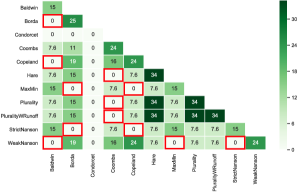
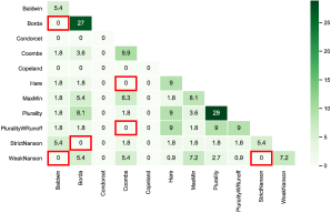
Figure 1: Percentage of profiles witnessing sure weak dominance manipulation for $(3,4)$ (left) and $(3,7)$ (right).

The numbers in Figure 1 represent the percentage of profiles that witness sure weak dominance manipulation for $(3,4)$ and $(3,7)$. For example, 7.6% of $(3,4)$-profiles witness sure weak dominance manipulation for $\{\texttt{Plurality},\texttt{Copeland}\}$. The numbers along the diagonal give the percentage of profiles witnessing weak dominance manipulation for a single voting method. The numbers highlighted in red identify pairs of voting methods that eliminate sure weak dominance manipulation according to Definition 3.4. For instance, 25% of the $(3,4)$-profiles witness weak dominance manipulation for Borda, 15% of the pointed $(3,4)$-profiles witness weak dominances manipulation for StrictNanson, but there are no instances of sure weak dominance manipulation for $\{\texttt{Borda},\texttt{StrictNanson}\}$.

To illustrate what happens with larger number of voters, we present in Figure 2 percentages for sure weak dominance manipulation for Borda alone and Borda paired with several other voting methods. The data for $(4,4)$ was obtain by exhaustive search, while the data for $(4,5)$–$(4,70)$ was obtained by generating 10,000 profiles for each $(4,m)$ using the Impartial Culture model.

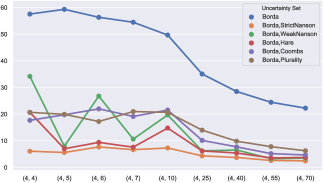
Figure 2: Percentage of $(4,m)$-profiles witnessing sure
weak dominance manipulation for Borda alone and
Borda paired with several other methods.

By exhaustive search from $(3,4)$–$(3,8)$, we find that $\{$Borda, Baldwin$\}$, $\{$Borda, StrictNanson$\}$, $\{$WeakNanson, Baldwin$\}$, and $\{$WeakNanson, StrictNanson$\}$ are not susceptible to sure weak dominance manipulation, while each method individually is. This raises the question of whether one can prove that for all $(3,m)$, those sets of methods eliminate sure weak dominance manipulation. Indeed, we will prove this result.

Lemma 3.5.

For any $n\geq 3$ and $m\geq 4$, Baldwin, Borda, StrictNanson, and WeakNanson are each susceptible to sure weak dominance manipulation for $(n,m)$.

Proof.

Given a $(3,m)$-profile $\mathbf{P}$, let $\mathbf{P}\uplus\mathbf{P}_{\_}2$ be the $(3,m+2)$-profile that results from adding to $\mathbf{P}$ two fresh voters with rankings $a\,b\,c$ and $c\,b\,a$, respectively. The rankings of candidates by Borda score in $\mathbf{P}$ and $\mathbf{P}\uplus\mathbf{P}_{\_}2$ are the same; the sets of candidates with the lowest Borda scores in $\mathbf{P}$ and $\mathbf{P}\uplus\mathbf{P}_{\_}2$ are the same; and the sets of candidates with less than average (resp. less than or equal to average) Borda scores in $\mathbf{P}$ and $\mathbf{P}\uplus\mathbf{P}_{\_}2$ are the same. Thus, the set of Borda (resp. Baldwin, StrictNanson, WeakNanson) winners does not change from $\mathbf{P}$ and $\mathbf{P}\uplus\mathbf{P}_{\_}2$. It follows that if $\mathbf{P}$ witnesses $\Delta$-manipulation for Borda (resp. Baldwin, StrictNanson, WeakNanson) by transitioning to $\mathbf{P}^{\prime}$, then $\mathbf{P}\uplus\mathbf{P}_{\_}2$ witnesses $\Delta$-manipulation for Borda (resp. Baldwin, StrictNanson, WeakNanson) by transitioning to $\mathbf{P}^{\prime}\uplus\mathbf{P}_{\_}2$. Thus, to prove that one of these voting methods is susceptible to $\Delta$-dominance manipulation for $(3,m)$ for any $m\geq 4$, it suffices to show this for $(3,4)$ and $(3,5)$, as susceptibility for all other pairs $(3,m)$ then follows by the preceding observation about $\mathbf{P}\uplus\mathbf{P}_{\_}2$. As we verified using our Python script, there are indeed $(3,4)$ and $(3,5)$ profiles witnessing weak dominance manipulability for all four methods individually.

For any $(n,m)$-profile $\mathbf{P}$, let $\mathbf{P}^{+}$ be the $(n+1,m)$-profile that results from adding to $\mathbf{P}$ a fresh candidate at the bottom of every voter’s ranking. The set of Borda (resp. Baldwin, StrictNanson, WeakNanson) winners does not change from $\mathbf{P}$ to $\mathbf{P}^{+}$. Thus, to prove that one of these methods is susceptible to $\Delta$-dominance manipulation for $(n,m)$ for any $n\geq 3$, it suffices to show this for $(3,m)$, as above.∎

The following main theorems, proved in the Appendix, show that uncertainty about the voting method can entirely eliminate sure weak dominance manipulation.

Theorem 3.6.

For any $m\geq 4$, the sets $\{\texttt{Borda},\texttt{Baldwin}\}$ and $\{\texttt{Borda},\texttt{StrictNanson}\}$ eliminate sure weak dominance manipulation for $(3,m)$.

Theorem 3.7.

For any $m\geq 4$, the sets $\{\texttt{WeakNanson},\texttt{Baldwin}\}$ and $\{\texttt{WeakNanson},\texttt{StrictNanson}\}$ eliminate sure weak dominance manipulation for $(3,m)$.

By contrast, already for $(3,5)$, $\{\texttt{Baldwin},\texttt{Borda},\texttt{StrictNanson},\texttt{WeakNanson}\}$ is susceptible to sure optimistic dominance and sure pessimistic dominance. We give an example for optimistic dominance, leaving pessimistic dominance as an exercise.

Example 3.8.

Let $\mathbf{P}$ be the following $(3,5)$ profile:

$1$	$2$	$3$	$4$	$5$
$a$	$a$	$b$	$c$	$c$
$b$	$b$	$a$	$b$	$b$
$c$	$c$	$c$	$a$	$a$

Baldwin, Borda, StrictNanson, and WeakNanson choose $\{b\}$. If voter 1 changes her ranking to $a\ c\ b$, then $\{a,b,c\}$ is the winning set for all four methods. Since $\{a,b,c\}>_{\_}{\mathbf{P}_{\_}1}^{Opt}\{b\}$, $(\mathbf{P},1)$ witnesses sure optimist dominance manipulability for $\{\texttt{Baldwin},\texttt{Borda},\texttt{StrictNanson},\texttt{WeakNanson}\}$.

For another contrast to Theorems 3.6-3.7, when we increase to 4 candidates, $\{$Baldwin, Borda, StrictNanson, WeakNanson$\}$ is susceptible to sure weak dominance manipulation.

Example 3.9.

Consider the following $(4,3)$-profile $\mathbf{P}$:

$1$	$2$	$3$
$a$	$b$	$c$
$b$	$d$	$a$
$c$	$c$	$b$
$d$	$a$	$d$

The Borda winning set is $\{b\}$, while the Baldwin, StrictNanson, and WeakNanson winning sets are all $\{a,b,c\}$. If voter 1 changes her ranking to $a\,d\,b\,c$, then the Borda winning set is $\{a,b\}$, while the Baldwin, StrictNanson, and WeakNanson winning sets are $\{a\}$. Since $\{a,b\}>_{\_}{\mathbf{P}_{\_}1}^{weak}\{b\}$ and $\{a\}>_{\_}{\mathbf{P}_{\_}1}^{weak}\{a,b,c\}$, $(\mathbf{P},1)$ witnesses sure weak dominance manipulability for $\{\texttt{Baldwin},\texttt{Borda},\texttt{StrictNanson},\texttt{WeakNanson}\}$.

3.2 The failure of the Duggan-Schwartz theorem for sets of voting methods

A natural analogue of the Duggan-Schwartz theorem [10] for sure manipulation of sets of voting methods would state that for any $(n,m)$ with $n\geq 3$ and set $S$ of methods, each of which is non-imposed and has no nominator, $S$ is susceptible to sure optimistic or pessimistic dominance manipulation for $(n,m)$. However, this statement is false, as shown by the following example verified by our Python script.

Example 3.10.

These sets of methods (which are non-imposed and have no nominator) eliminate sure optimistic and pessimistic dominance manipulation for $(3,6)$: $\{$Baldwin, Condorcet$\}$, $\{$Condorcet, Copeland$\}$, $\{$Condorcet, MaxMin$\}$, $\{$Condorcet, StrictNanson$\}$, and $\{$Condorcet, WeakNanson$\}$.

3.3 Cases where three methods are needed for elimination

So far we have only considered sets of two voting methods. But in some cases three voting methods are needed to eliminate sure manipulation. We saw in Example 3.9 that $\{\texttt{Borda},\texttt{Baldwin}\}$ is susceptible to sure weak dominance manipulation for $(4,3)$. However, adding Coombs to $\{\texttt{Borda},\texttt{Baldwin}\}$ eliminates sure weak dominance manipulation, as verified by our Python script (which also finds profiles witnessing sure weak dominance manipulability for $\{\texttt{Borda},\texttt{Coombs}\}$ and $\{\texttt{Coombs},\texttt{Baldwin}\}$).

Fact 3.11.

$\{\texttt{Borda},\texttt{Coombs},\texttt{Baldwin}\}$ eliminates sure weak dominance manipulation for $(4,3)$.

3.4 $(n,m)$ for which sure manipulation cannot be eliminated

So far we have focused on eliminating sure manipulation using uncertainty about the voting method. However, as the following result shows, eliminating sure manipulation is not always possible.

Proposition 3.12.

For every $(n,m)$, there are $n^{\prime}>n$ and $m^{\prime}>m$ such that every nonempty subset of $\mathsf{Methods}\setminus\{\texttt{Condorcet}\}$ is susceptible to sure weak dominance manipulation for $(n^{\prime},m^{\prime})$.

Proof.

First, we claim that if there is one $(n,m)$-profile that witnesses sure weak dominance manipulability for every nonempty subset of $\mathsf{Methods}\setminus\{\texttt{Condorcet}\}$, then for all $k\in\mathbb{N}$, there is an $(n,m+24k)$-profile that does so. For any profile $\mathbf{P}$, let $\mathbf{P}\uplus\mathbf{P}_{\_}{24}$ be the result of adding 24 new voters to $\mathbf{P}$, one with each of the possible 24 rankings of $\{a,b,c,d\}$. It is easy to see that for any $f\in\mathsf{Methods}$, $f(\mathbf{P})=f(\mathbf{P}\uplus\mathbf{P}_{\_}{24})$. It follows that if $\mathbf{P}$ witnesses sure $\Delta$-dominance manipulability for $S$ by transitioning to $\mathbf{P}^{\prime}$, then so does $\mathbf{P}\uplus\mathbf{P}_{\_}{24}$ by transitioning to $\mathbf{P}^{\prime}\uplus\mathbf{P}_{\_}{24}$. In addition, using the construction from $\mathbf{P}$ to $\mathbf{P}^{+}$ in the proof of Lemma 3.5, we can increase the number $n$ of candidates, since for any $f\in\mathsf{Methods}$, $f(\mathbf{P})=f(\mathbf{P}^{+})$. Now consider the following $(4,4)$-profile $\mathbf{P}$:

$1$	$2$	$3$	$4$
$a$	$b$	$c$	$c$
$b$	$d$	$a$	$a$
$c$	$c$	$b$	$b$
$d$	$a$	$d$	$d$

Every method in $\mathsf{Methods}\setminus\{\texttt{Condorcet}\}$ chooses $\{c\}$ as the set of winners. If voter 1 changes to $b\,d\,c\,a$, then the winning set for all methods in ${\mathsf{Method}\setminus\{\texttt{Condorcet}\}}$ becomes $\{b,c\}$. Since $\{b,c\}>_{\_}{\mathbf{P}_{\_}1}^{weak}\{c\}$, $(\mathbf{P},1)$ witnesses sure weak dominance manipulability for any nonempty subset of $\mathsf{Method}\setminus\{\texttt{Condorcet}\}$.∎

3.5 Reduction without elimination

Even when eliminating sure manipulation is not possible, one may hope to reduce it. For example, in Figures 1 and 2, there are a number of cases in which a pair of methods does not eliminate sure weak dominance manipulation but does reduce the number of profiles witnessing sure weak dominance manipulation relative to either method individually. This motivates the following notions.

Definition 3.13.

For any sets $S$ and $S^{\prime}$ of voting methods, $S$ is less susceptible to sure $\Delta$-manipulation than $S^{\prime}$ for $(n,m)$-profiles (resp. pointed $(n,m)$-profiles) iff there are fewer $(n,m)$-profiles (resp. pointed $(n,m)$-profiles) witnessing sure $\Delta$-manipulation for $S$ than there are for $S^{\prime}$.

Definition 3.14.

A set $S$ of methods improves on all its subsets with respect to sure $\Delta$-manipulation for $(n,m)$ iff $S$ is less susceptible to sure $\Delta$-manipulation for $(n,m)$-profiles than any nonempty $S^{\prime}\subsetneq S$.

Such improvement is especially pronounced with optimistic and pessimistic dominance, as in Figure 3.

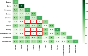
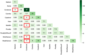
Figure 3: Percentage of profiles witnessing sure optimistic dominance manipulation for $(3,7)$ (left) and sure pessimistic dominance manipulation for $(3,6)$ (right).

Even if a set $S$ does not improve on all of its subsets, that $S$ is less susceptible to sure $\Delta$-manipulation than one of its subset may still be significant. An election designer who intends to use method $f$ may wish to leave voters uncertain between $f$ and $f^{\prime}$ in order to reduce the chance that voters will surely manipulate, relative to what would happen if voters knew the method was $f$, even if there is no reduction relative to what would happen if the planner intended to use $f^{\prime}$ and voters knew this. For example, in Figure 1 for $(3,7)$, someone intending to use Plurality could reduce the percentage of profiles in which a voter will surely manipulate from 29% to 9% by leaving the voter uncertain between Plurality and Hare, even though an election designer intending to use Hare would have no incentive to do so, since the percentage of profiles witnessing sure manipulation for Hare by itself is already 9%.

A striking pattern in Figures 1, 2, and 3 is that pairing Borda with another method leads to significant reductions in sure dominance manipulation. Using one or more methods to help reduce manipulation for a preferred method is even more important in the case of safe manipulation discussed next.

4 Safe manipulation

We now turn to a less conservative approach to strategic voting under uncertainty about the voting method: submit an insincere ranking whenever you know that doing so will lead to an outcome that is at least as good and might lead to a better outcome.

Definition 4.1.

Let $(\mathbf{P},i)$ be a pointed profile, $\Delta$ a dominance notion, and $S$ a set of voting methods. Then $(\mathbf{P},i)$ witnesses safe $\Delta$-manipulability for $S$ iff there is a profile $\mathbf{P}^{\prime}$ differing from $\mathbf{P}$ only in $i$’s ballot such that: $\forall f\in S:f(\mathbf{P}^{\prime})\geq_{\_}{\mathbf{P}_{\_}i}^{\Delta}f(\mathbf{P})\,\mbox{ and }\,\exists f\in S:f(\mathbf{P}^{\prime})>_{\_}{\mathbf{P}_{\_}i}^{\Delta}f(\mathbf{P})$. We then say that $(\mathbf{P},i)$ witnesses safe $\Delta$-manipulability for $S$ by transitioning to $\mathbf{P}^{\prime}$. A profile $\mathbf{P}$ witnesses safe $\Delta$-manipulability for $S$ iff there is an $i\in V$ such that $(\mathbf{P},i)$ witnesses safe $\Delta$-manipulability for $S$.

Remark 4.2.

A variant of safe manipulability, which we will call harmless manipulability, says that you should submit an insincere ranking whenever you know that doing so will not lead to a worse outcome and might lead to a better outcome: $\forall f\in S:f(\mathbf{P}^{\prime})\not<_{\_}{\mathbf{P}_{\_}i}^{\Delta}f(\mathbf{P})\,\mbox{ and }\,\exists f\in S:f(\mathbf{P}^{\prime})>_{\_}{\mathbf{P}_{\_}i}^{\Delta}f(\mathbf{P})$. Since $f(\mathbf{P}^{\prime})\not<_{\_}{\mathbf{P}_{\_}i}^{weak}f(\mathbf{P})$ does not imply $f(\mathbf{P}^{\prime})\geq_{\_}{\mathbf{P}_{\_}i}^{weak}f(\mathbf{P})$, harmless weak dominance manipulability does not imply safe weak dominance manipulability for a given $(\mathbf{P},i)$ transitioning to $\mathbf{P}^{\prime}$. But for pessimistic and optimistic dominance, harmless and safe manipulability are equivalent.

For certain profiles and uncertainty sets $S$, submitting an insincere ranking may lead to a better outcome with one method in $S$ but a worse outcome with another method in $S$, in which case it is not safe to manipulate using that insincere ranking.

Example 4.3.

Let $\mathbf{P}$ be the following $(3,5)$-profile:

$1$	$2$	$3$	$4$	$5$
$c$	$a$	$b$	$c$	$a$
$b$	$c$	$a$	$b$	$c$
$a$	$b$	$c$	$a$	$b$

Here $\texttt{Hare}(\mathbf{P})=\{a\}$, $\texttt{Borda}(\mathbf{P})=\{c\}$, and $\texttt{MaxMin}(\mathbf{P})=\{a,c\}$. Suppose voter 1 changes her ranking to $b\ a\ c$, resulting in $\mathbf{P}^{\prime}$. Then $\texttt{Hare}(\mathbf{P}^{\prime})=\{b\}$, $\texttt{Borda}(\mathbf{P}^{\prime})=\{a\}$, and $\texttt{MaxMin}(\mathbf{P}^{\prime})=\{a,b\}$. Since $\{b\}>_{\_}\mathbf{P}^{weak}\{a\}$, voter 1 has an incentive to manipulate with Hare. But voter 1 does not have an incentive to manipulate with Borda, since $\{c\}>^{weak}_{\_}{\mathbf{P}_{\_}1}\{a\}$, or MaxMin, since $\{a,b\}\not\geq^{weak}_{\_}{\mathbf{P}_{\_}1}\{a,c\}$.

Thus, $(\mathbf{P},1)$ does not witness safe weak dominance manipulation for Borda together with any nonempty subset of $\{\texttt{Hare},\texttt{MaxMin}\}$.

It seems too much to hope to eliminate safe manipulation by adding reasonable methods to $S$; for this would require that for every profile in which a manipulation results in a better outcome for one method in $S$, it results in a worse outcome for another method in $S$, which seems unlikely to hold for a set of reasonable methods. However, one can eliminate safe manipulation by adding methods that would be considered unreasonable by themselves.

Example 4.4.

For any distinct $x,y\in C$ and $i\in V$, let $f_{\_}{x,y,i}$ be the method such that $f_{\_}{x,y,i}(\mathbf{P})$ selects as the winner whichever of $x$ and $y$ is ranked higher according to $\mathbf{P}_{\_}i$ (cf. [27]). It is easy to see that if $S$ contains $f_{\_}{x,y,i}$ for each distinct $x,y\in C$, then $i$ cannot safely manipulate with $S$.

Although eliminating safe manipulation with reasonable methods may be too much to hope for, one can reduce safe manipulation. Thus, we are interested in the following analogue of Definition 3.13.

Definition 4.5.

For any sets $S$ and $S^{\prime}$ of voting methods, $S$ is less susceptible to safe $\Delta$-manipulation than $S^{\prime}$ for $(n,m)$-profiles (resp. pointed $(n,m)$-profiles) iff there are fewer $(n,m)$-profiles (resp. pointed $(n,m)$-profiles) witnessing sure safe $\Delta$-manipulation for $S$ than there are for $S^{\prime}$.

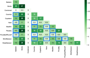
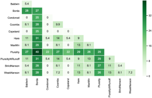
Figure 4: Percentage of profiles witnessing safe weak dominance manipulation for $(3,6)$ (left) and $(3,7)$ (right).

Figure 4 shows the percentage of profiles witnessing safe weak dominance manipulation for $(3,6)$ and $(3,7)$ for sets of two voting methods. All of the following can happen: (1) Unlike with sure manipulation, with safe manipulation a voter who is uncertain between methods $f$ and $f^{\prime}$ may have an incentive to manipulate on more profiles than a voter who knows the method is $f$ and more profiles than a voter who knows the method is $f^{\prime}$. E.g., this happens for $(3,7)$ when $f=\mathtt{Borda}$ and $f^{\prime}=\mathtt{Hare}$. (2) A voter who is uncertain between methods $f$ and $f^{\prime}$ may have an incentive to manipulate on fewer profiles than a voter who knows the method is $f$ and fewer profiles than a voter who knows the method if $f^{\prime}$. E.g., this happens for $(3,6)$ when $f=\mathtt{Coombs}$ and $f^{\prime}=\mathtt{Hare}$. In Figure 4, all examples of this phenomenon are indicated with the blue boxes. For $(3,7)$, there are no examples.

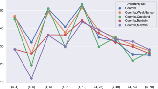
Figure 5: Percentage of $(4,m)$-profiles witnessing safe
weak dominance manipulation for Coombs alone and
Coombs paired with several other methods.
 

(3) A voter who is uncertain between methods $f$ and $f^{\prime}$ may have an incentive to manipulate on fewer profiles than a voter who knows the method is $f$ but more profiles than a voter who knows the method is $f^{\prime}$. E.g., this happens with $(3,6)$ when $f=\mathtt{Borda}$ and $f^{\prime}=\mathtt{Hare}$. In case (3), an election designer who intends to use method $f$ may decide to leave voters uncertain between $f$ and $f^{\prime}$ in order to decrease the chance that voters will safely manipulate (cf. the end of Section 3.5). E.g., Figure 5 shows how an election designer intending to use Coombs could pair Coombs with several other methods to form an uncertainty set of two methods in order to decrease the percentage of profiles in which a voter will safely manipulate.

5 Expected manipulation

Our last approach to strategic voting under uncertainty about the voting method is the most liberal: assuming one’s uncertainty about the voting method is given by a lottery on the set of voting methods, submit an insincere ranking if and only if doing so is more likely to lead to a better outcome than to lead to a worse outcome. Recall that a lottery on a set $Y$ is a function $\nu:Y\to[0,1]$ such that $\sum_{\_}{y\in Y}\nu(y)=1$. For $X\subseteq Y$, let $\nu(X)=\sum_{\_}{x\in X}\nu(x)$.

Definition 5.1.

Let $(\mathbf{P},i)$ be a pointed profile, $\Delta$ a dominance notion, $S$ a set of voting methods, and $\nu$ a lottery on $S$. Then $(\mathbf{P},i)$ witnesses $\nu$-expected $\Delta$-manipulability for $S$ if and only if there is a profile $\mathbf{P}^{\prime}$ differing from $\mathbf{P}$ only in $i$’s ballot such that $\nu(\{f\in S\mid f(\mathbf{P}^{\prime})>_{\_}{\mathbf{P}_{\_}i}^{\Delta}f(\mathbf{P})\})>\nu(\{f\in S\mid f(\mathbf{P}^{\prime})<_{\_}{\mathbf{P}_{\_}i}^{\Delta}f(\mathbf{P})\})$. Then we say $(\mathbf{P},i)$ witnesses $\nu$-expected $\Delta$-manipulability for $S$ by transitioning to $\mathbf{P}^{\prime}$.

For simplicity, here we focus on $\nu$ being the uniform lottery on $S$, in which case we simply speak of ‘expected $\Delta$-manipulability’ instead of ‘$\nu$-expected $\Delta$-manipulability’. For $\nu$ uniform, this amounts to simply counting the number of voting methods in $S$ that lead to a better outcome vs. a worse outcome.

Example 5.2.

The pointed profile $(\mathbf{P},1)$ in Example 4.3 does not witness expected weak dominance manipulability for $\{\mathtt{Borda},\mathtt{Hare}\}$ by transitioning to $\mathbf{P}^{\prime}$ since voter 1’s manipulation results in a better outcome according to one method (Hare) but a worse outcome according to another method (Borda). However, like Hare, Baldwin chooses $\{a\}$ as the set of winners in $\mathbf{P}$ and $\{b\}$ as the set in $\mathbf{P}^{\prime}$. Hence $(\mathbf{P},1)$ witnesses expected weak dominance manipulability for $\{\mathtt{Baldwin},\mathtt{Borda},\mathtt{Hare}\}$ by transitioning to $\mathbf{P}^{\prime}$, as two methods lead to a better outcome and only one leads to a worse outcome.

The following fact is immediate from the definitions.

Fact 5.3.

If $(\mathbf{P},i)$ witnesses safe $\Delta$-dominance manipulability for $S$, then $(\mathbf{P},i)$ witnesses expected $\Delta$-dominance manipulability for $S$.

The converse of Fact 5.3 does not hold, as shown by Example 5.2. But for $|S|=2$ expected weak dominance manipulability is equivalent to harmless weak dominance manipulability (recall Remark 4.2).

Using the obvious notion of less susceptible to expected $\Delta$-dominance manipulation analogous to Definitions 3.13 and 4.5, we have the following result, inspired by [27], showing how adding a method to the set $S$ may reduce expected manipulation.

Proposition 5.4.

Suppose $S$ is a set of voting methods such that for some $f\in S$, $(n,m)$, pointed $(n,m)$-profile $(\mathbf{P},i)$, and $a,b\in C$, (1) $(\mathbf{P},i)$ witnesses weak dominance manipulability for $f$, and (2) for any $\mathbf{P}^{\prime}$ differing from $\mathbf{P}$ only in $i$’s ranking, if $(\mathbf{P},i)$ witnesses weak dominance manipulability for $f$ by transitioning to $\mathbf{P}^{\prime}$, then $\mathbf{P}^{\prime}$ differs from $\mathbf{P}$ in $i$’s ranking of $a$ vs. $b$, and for all $g\in S\setminus\{f\}$, $g(\mathbf{P})=g(\mathbf{P}^{\prime})$. Then where $f_{\_}{a,b,i}$ is the method defined in Example 4.4, $S\cup\{f_{\_}{a,b,i}\}$ is less susceptible to expected weak dominance manipulation than $S$ for pointed $(n,m)$-profiles.

Proof.

The key properties of $f_{\_}{a,b,i}$ are that (i) there are no profiles $\mathbf{P}$ and $\mathbf{P}^{\prime}$ differing only in $i$’s ranking such that we have $f_{\_}{a,b,i}(\mathbf{P}^{\prime})>^{weak}_{\_}{\mathbf{P}_{\_}i}f_{\_}{a,b,i}(\mathbf{P})$, and (ii) if $\mathbf{P}$ and $\mathbf{P}^{\prime}$ differ in $i$’s ranking of $a$ vs. $b$, then $f_{\_}{a,b,i}(\mathbf{P}^{\prime})<^{weak}_{\_}{\mathbf{P}_{\_}i}f_{\_}{a,b,i}(\mathbf{P})$. It follows from (i) that any pointed profile witnessing expected weak dominance manipulability for ${S\cup\{f_{\_}{a,b,i}\}}$ also witnesses expected weak dominance manipulability for $S$. Thus, to prove the proposition, we need only find a pointed profile witnessing expected weak dominance manipulability for $S$ but not ${S\cup\{f_{\_}{a,b,i}\}}$. By assumption, there is a pointed $(n,m)$-profile $(\mathbf{P},i)$ and $a,b\in C$ satisfying items (1) and (2) of the proposition. Given (1), consider any $\mathbf{P}^{\prime}$ such that $(\mathbf{P},i)$ witnesses weak dominance manipulability for $f$ by transitioning to $\mathbf{P}^{\prime}$. It then follows by (2) that $(\mathbf{P},i)$ witnesses expected weak dominance manipulability for $S$ by transitioning to $\mathbf{P}^{\prime}$. However, we claim that $(\mathbf{P},i)$ does not witness expected weak dominance manipulability for $S\cup\{f_{\_}{a,b,i}\}$ by transitioning to $\mathbf{P}^{\prime}$. This follows from the facts that $f$ and $f_{\_}{a,b,i}$ are equally likely according to the uniform measure, $\{h\in S\cup\{f_{\_}{a,b,i}\}\mid h(\mathbf{P}^{\prime})<^{weak}_{\_}{\mathbf{P}_{\_}i}h(\mathbf{P})\}=\{f_{\_}{a,b,i}\}$ by (2) and (ii), and $\{h\in S\cup\{f_{\_}{a,b,i}\}\mid h(\mathbf{P}^{\prime})>^{weak}_{\_}{\mathbf{P}_{\_}i}h(\mathbf{P})\}=\{f\}$ by (2).∎

We conclude this section with an example in which the conditions of Proposition 5.4 apply.

Example 5.5.

Consider the following $(3,5)$-profile $\mathbf{P}$:

$1$	$2$	$3$	$4$	$5$
$c$	$c$	$a$	$a$	$a$
$a$	$a$	$c$	$c$	$c$
$b$	$b$	$b$	$b$	$b$

Let $S=\{\texttt{Borda},\texttt{Coombs}\}$. $(\mathbf{P},i)$ witnesses the weak manipulability of Borda by transitioning to the profile $\mathbf{P^{\prime}}$ in which $i$’s new ranking is $c\,b\,a$, as the Borda winning set in $\mathbf{P}$ is $\{a\}$, the Borda winning set in $\mathbf{P}^{\prime}$ is $\{a,c\}$, and $\{a,c\}>^{weak}_{\_}{\mathbf{P}_{\_}1}\{a\}$.

Moreover, this is the only $\mathbf{P}^{\prime}$ differing from $\mathbf{P}$ only in $i$’s ranking such that $(\mathbf{P},i)$ witnesses the weak manipulability of Borda by transitioning to $\mathbf{P^{\prime}}$. Finally, the winning set for Coombs in both $\mathbf{P}$ and $\mathbf{P}^{\prime}$ is $\{a\}$. Thus, the conditions of Proposition 5.4 are satisfied for $f=\mathtt{Borda}$, so $\{\texttt{Borda},\texttt{Coombs},f_{\_}{a,b,i}\}$ is less susceptible to expected weak dominance manipulation than $\{\texttt{Borda},\texttt{Coombs}\}$.

6 Relation to probabilistic social choice

In this section, we briefly relate our work to strategic voting in the setting of probabilistic social choice.

Definition 6.1.

A probabilistic social choice function (PSCF) is a function $F$ assigning to each profile $\mathbf{P}$ a lottery $F(\mathbf{P})$ on $C$.

To define manipulation of PSCFs, we need a notion of when a voter prefers one lottery to another. Among many possible options (see, e.g., [5, Sec. 1.3.2]), the following is popular.

Definition 6.2.

Let $\mu$ and $\mu^{\prime}$ be lotteries on $C$ and $(\mathbf{P},i)$ a pointed profile. We say that $\mu$ stochastically dominates $\mu^{\prime}$ in $(\mathbf{P},i)$ if and only if for every $x\in C$, the probability that $\mu$ selects a candidate ranked at least as highly as $x$ by $i$ is greater than or equal to the probability that $\mu^{\prime}$ selects a candidate ranked at least as highly as $x$ by $i$:

$$\forall x\in C:\underset{y\,:\,y\mathbf{R}_{\_}ix}{\sum}\mu(y)\geq\underset{y\,:\,y\mathbf{R}_{\_}ix}{\sum}\mu^{\prime}(y).$$

We write $\mu\succsim_{\_}{\mathbf{P}_{\_}i}\mu^{\prime}$ if $\mu$ stochastically dominates $\mu^{\prime}$ in $(\mathbf{P},i)$ and $\mu\succ_{\_}{\mathbf{P}_{\_}i}\mu^{\prime}$ if $\mu\succsim_{\_}{\mathbf{P}_{\_}i}\mu^{\prime}$ but $\mu^{\prime}\not\succsim_{\_}{\mathbf{P}_{\_}i}\mu$.

Note that $\mu\succsim_{\_}{\mathbf{P}_{\_}i}\mu^{\prime}$ if and only if for every utility function on $C$ that is compatible with $\mathbf{P}_{\_}i$, the expected utility of $\mu$ is at least as great as the expected utility of $\mu^{\prime}$ (see, e.g., [4, p. 302-3]).

Definition 6.3.

Let $F$ be a PSCF. A pointed profile $(\mathbf{P},i)$ witnesses stochastic dominance manipulability for $F$ if and only if there is a profile $\mathbf{P}^{\prime}$ differing only in $i$’s ranking such that $F(\mathbf{P}^{\prime})\succ_{\_}{\mathbf{P}_{\_}i}F(\mathbf{P})$. We then say that $(\mathbf{P},i)$ witnesses stochastic dominance manipulability for $F$ by transitioning to $\mathbf{P}^{\prime}$.

For results on stochastic dominance manipulability, see [5].

To relate the above notions to this paper, we observe how any set $S$ of voting methods gives rise to a PSCF, assuming that (i) each method in $S$ is equally likely to be used and (ii) each candidate in the set of winners selected by a method is equally likely to be chosen as the unique winner by a tiebreaking mechanism. Then the probability that a given candidate $a\in C$ will be chosen as the winner is:

$$Pr(a\mbox{ wins}) = \underset{f\in S}{\sum}Pr(a\mbox{ wins}\,|\,f\mbox{ is used})\times Pr(f\mbox{ is used})$$

$$= \underset{\underset{a\in f(\mathbf{P})}{f\in S}}{\sum}Pr(a\mbox{ wins}\,|\,f\mbox{ is used})\times Pr(f\mbox{ is used})+\underset{\underset{a\not\in f(\mathbf{P})}{f\in S}}{\sum}Pr(a\mbox{ wins}\,|\,f\mbox{ is used})\times Pr(f\mbox{ is used})$$

$$= \Big{(}\underset{\underset{a\in f(\mathbf{P})}{f\in S}}{\sum}\frac{1}{|f(\mathbf{P})|}\times\frac{1}{|S|}\Big{)}+\Big{(}\underset{\underset{a\not\in f(\mathbf{P})}{f\in S}}{\sum}0\times\frac{1}{|S|}\Big{)}\quad=\quad\underset{\underset{a\in f(\mathbf{P})}{f\in S}}{\sum}\frac{1}{|f(\mathbf{P})|}\times\frac{1}{|S|}.$$

Thus, for a profile $\mathbf{P}$ and set $S$ of voting methods, we define the lottery $\mu^{\mathbf{P}}_{\_}S$ on $C$ by

$$\mu^{\mathbf{P}}_{\_}S(a)=\underset{\underset{a\in f(\mathbf{P})}{f\in S}}{\sum}\frac{1}{|f(\mathbf{P})|}\times\frac{1}{|S|}.$$

Finally, for any set $S$ of voting methods, we define the PSCF $F_{\_}S$ by $F_{\_}S(\mathbf{P})=\mu^{\mathbf{P}}_{\_}S$.

Remark 6.4.

For any set $S$ of voting methods and lottery $\nu$ on $S$, one can define a PSCF $F_{\_}{S,\nu}$ in the obvious way by weighting the methods in $S$ according to $\nu$ (and one can modify assumption (ii) with a non-uniform measure for tiebreaking). For simplicity, here we focus on the uniform measure on $S$.

The following fact can be verified from the definitions.

Fact 6.5.

If $(\mathbf{P},i)$ witnesses safe weak dominance manipulation for $S$ by transitioning to $\mathbf{P}^{\prime}$, then $(\mathbf{P},i)$ witnesses stochastic dominance manipulation for $F_{\_}S$ by transitioning to $\mathbf{P}^{\prime}$.

However, stochastic manipulation does not imply safe weak manipulation.

Example 6.6.

Consider the following $(3,4)$-profile $\mathbf{P}$ for $C=\{a,b,c\}$ and $V=\{1,2,3,4\}$:

$1$	$2$	$3$	$4$
$a$	$a$	$b$	$b$
$b$	$c$	$a$	$a$
$c$	$b$	$c$	$c$

The Coombs, Copeland, and Hare winning set is $\{a,b\}$. If voter 1 changes to the ranking $c\,a\,b$, transitioning to the profile $\mathbf{P}^{\prime}$, then the new winning set for Coombs and Copeland is $\{a\}$ and the new winning set for Hare is $\{b\}$. Note that $\{a\}>_{\_}{\mathbf{P}_{\_}1}^{weak}\{a,b\}$ and $\{a,b\}>_{\_}{\mathbf{P}_{\_}1}^{weak}\{b\}$, so voter 1’s new ranking leads to a better weak dominance outcome according to Coombs and Copeland but a worse weak dominance outcome according to Hare.

Thus, $(\mathbf{P},1)$ does not witness safe weak dominance manipulability by transitioning to $\mathbf{P}^{\prime}$.

Let $S=\{\texttt{Coombs},\texttt{Copeland},\texttt{Hare}\}$. The lottery $F_{\_}S(\mathbf{P})$ is [$a:1/2$, $b:1/2$, $c:0$]. The lottery $F_{\_}S(\mathbf{P}^{\prime})$ is [$a:2/3$, $b:1/3$, $c:0$]. As voter $1$’s ranking in $\mathbf{P}$ is $a\,b\,c$, $F_{\_}S(\mathbf{P}^{\prime})$ stochastically dominates $F_{\_}S(\mathbf{P})$, since the probability according to $F_{\_}S(\mathbf{P}^{\prime})$ of selecting a candidate at least as good as $b$ is equal to the probability according to $F_{\_}S(\mathbf{P})$ (both are 1), and the probability according to $F_{\_}S(\mathbf{P}^{\prime})$ of selecting a candidate at least as good as $a$ (probability $2/3$) is greater than the probability according to $F_{\_}S(\mathbf{P})$ (probability $1/2$). So $(\mathbf{P},1)$ witnesses stochastic dominance manipulability for $F_{\_}S(\mathbf{P})$ by transitioning to $\mathbf{P}^{\prime}$.

It is easy to see abstractly that stochastic dominance manipulation also does not imply expected weak dominance manipulation: e.g., if $S=\{f_{\_}1,f_{\_}2\}$ and the transition from $(\mathbf{P},i)$ to $\mathbf{P}$ is such that ${f_{\_}1(\mathbf{P})<_{\_}{\mathbf{P}_{\_}i}^{weak}f_{\_}1(\mathbf{P}^{\prime})}$ and $f_{\_}2(\mathbf{P})>_{\_}{\mathbf{P}_{\_}i}^{weak}f_{\_}2(\mathbf{P}^{\prime})$, then the transition does not witness expected weak manipulation, but the amount by which $f_{\_}1$ increases the probability of getting a preferred candidate may be greater than the amount by which $f_{\_}2$ decreases the probability of getting a preferred candidate, so that the lottery $F_{\_}{f_{\_}1,f_{\_}2}(\mathbf{P}^{\prime})$ stochastically dominates the lottery $F_{\_}{f_{\_}1,f_{\_}2}(\mathbf{P})$. The same idea applies for more than two methods. It remains to be seen whether an example of this kind exists with standard voting methods.

We can, however, use standard methods to show that expected weak dominance manipulation does not imply stochastic weak dominance manipulation.

Example 6.7.

Let $\mathbf{P}$ and $\mathbf{P}^{\prime}$ be the profiles in Example 4.3 and $S=\{\mathtt{Baldwin},\mathtt{Borda},\mathtt{Hare}\}$. In $\mathbf{P}$, Baldwin and Hare select $a$ as the winner, while Borda selects $c$ as the winner. Thus, the lottery $F_{\_}S(\mathbf{P})$ is [$a:2/3$, $b:0$, $c:1/3$]. In $\mathbf{P}^{\prime}$, Baldwin and Hare select $b$ as the winner, while Borda selects $a$ as the winner. Thus, the lottery $F_{\_}S(\mathbf{P}^{\prime})$ is [$a:1/3$, $b:2/3$, $c:0$]. As voter $1$’s ranking in $\mathbf{P}$ is $c\,b\,a$, $F_{\_}S(\mathbf{P}^{\prime})$ does not stochastically dominate $F_{\_}S(\mathbf{P})$, since the probability according to $F_{\_}S(\mathbf{P}^{\prime})$ of selecting a candidate at least as good as $c$ is not greater than or equal to the probability according to $F_{\_}S(\mathbf{P})$ of selecting a candidate at least as good as $c$. Thus, $(\mathbf{P},1)$ does not witness stochastic dominance manipulability for $F_{\_}S(\mathbf{P})$ by transitioning to $\mathbf{P}^{\prime}$. However, as two of the three methods in $S$ lead to a better set of winners (in the sense of weak dominance) in $\mathbf{P}^{\prime}$ than in $\mathbf{P}$ according to voter $1$’s ranking in $\mathbf{P}$, $(\mathbf{P},1)$ does witness expected weak dominance manipulability for $\{\mathtt{Baldwin},\mathtt{Borda},\mathtt{Hare}\}$ by transitioning to $\mathbf{P}^{\prime}$.

7 Conclusion

In this paper, we have shown that uncertainty about the voting method can be used as a barrier to manipulation. Considering such uncertainty led to three decision rules that voters may use to decide when to manipulate: sure, safe, and expected manipulation. Related issues arise when studying probabilistic voting methods, though Section 6 shows that our notions of sure, safe, and expected manipulation do not collapse to a standard notion of stochastic manipulation of probabilistic voting methods.

This initial study relied heavily on computer searches. Two natural next steps are (i) to prove additional possibility (or impossibility) theorems, like our Theorems 3.6-3.7, and (ii) to incorporate uncertainty about voting methods into the asymptotic analysis of strategic voting as the number of candidates or voters increases (see, e.g., [34, 24]). Finally, a full analysis should take into account both uncertainty about the voting method and uncertainty about how others will vote.

Appendix A Proof of Theorem 3.6

In this appendix, we prove Theorem 3.6: for any $m\geq 4$, the sets $\{$Borda, Baldwin$\}$ and $\{$Borda, StrictNanson$\}$ eliminate sure weak dominance manipulation for $(3,m)$.

Proof.

Given Lemma 3.5, we need only show that the two sets of methods are not susceptible to sure weak dominance manipulation for $(3,m)$. Toward a contradiction, suppose $(\mathbf{P},i)$ is a pointed $(3,m)$-profile witnessing sure weak dominance manipulation for either of the two sets by transitioning to a profile $\mathbf{P}^{\prime}$. Suppose $i$’s ballot in $\mathbf{P}$ is $\alpha\beta\gamma$.

Claim 1: the Borda winning set in $\mathbf{P}^{\prime}$ does not contain all three candidates. This follows by analyzing the possible sets of Borda winners in P. A three-way tie $\{\alpha,\beta,\gamma\}$ does not weakly dominate any of the following sets for $i$: $\{\alpha\}$, $\{\beta\}$, $\{\alpha,\beta\}$, $\{\alpha,\gamma\}$, $\{\alpha,\beta,\gamma\}$. This leaves only the winning sets $\{\beta,\gamma\}$ and $\{\gamma\}$ to consider. But voter $i$ cannot manipulate so as to change the set of Borda winners from $\{\beta,\gamma\}$ to $\{\alpha,\beta,\gamma\}$; for the Borda scores of $\beta$ and $\gamma$ must still be tied in $\mathbf{P}^{\prime}$, so $i$’s ranking in $\mathbf{P}^{\prime}$ must be $\beta\gamma\alpha$, which decreases $\alpha$’s Borda score. In addition, voter $i$ cannot manipulate so as to change the set of Borda winners from $\{\gamma\}$ to $\{\alpha,\beta,\gamma\}$. For if $i$ ranks $\gamma$ higher in $\mathbf{P}^{\prime}$, then $\gamma$’s Borda score increases by at least one, and no other candidate’s Borda score increases by more than one, so the set of winners is still $\{\gamma\}$; hence $i$’s ranking in $\mathbf{P}^{\prime}$ must be $\beta\alpha\gamma$, but this fails to add $\alpha$ to the set of winners.

Label the candidates in order of ascending Borda score in $\mathbf{P}^{\prime}$ as $\varphi$, $\psi$, and $\chi$. Thus, by Claim 1,

$$B^{\prime}(\varphi)<B^{\prime}(\psi)\leq B^{\prime}(\chi)\mbox{ or }$$ (1)

$$B^{\prime}(\varphi)=B^{\prime}(\psi)<B^{\prime}(\chi),$$ (2)

where $B^{\prime}$ indicates the Borda score in $\mathbf{P}^{\prime}$. Let $B(\varphi),B(\psi),B(\chi)$ be the Borda scores of $\varphi$, $\psi$, and $\chi$ in $\mathbf{P}$.

Claim 2: $i$’s ranking changes from $\mathbf{P}$ to $\mathbf{P}^{\prime}$ either by switching her 1st and 2nd placed candidates or by switching her 2nd and 3rd candidates; thus, one candidate’s Borda score remains the same, and no candidate’s Borda score changes by more than one point. Suppose for a contradiction that $i$’s 3rd place candidate in $\mathbf{P}$ is her 1st place candidate in $\mathbf{P}^{\prime}$ or her 1st place candidate in $\mathbf{P}$ is her 3rd place candidate in $\mathbf{P}^{\prime}$. Then since $i$’s ranking in $\mathbf{P}$ is $\alpha\beta\gamma$, we have that $i$’s ranking in $\mathbf{P}^{\prime}$ is either $\gamma\beta\alpha$, $\gamma\alpha\beta$, or $\beta\gamma\alpha$. But we claim $i$ does not have an incentive to transition to any of these rankings from the original ranking $\alpha\beta\gamma$. The first two transitions are such that the only candidate to increase in Borda score is $i$’s last place candidate, which never improves the winning set for $i$. The transition from $\alpha\beta\gamma$ to $\beta\gamma\alpha$ does not improve the winning set if the winning set in $\mathbf{P}$ contains $\alpha$; and if the winning set in $\mathbf{P}$ is $\{\beta\}$, $\{\gamma\}$, or $\{\beta,\gamma\}$, again the transition from $\alpha\beta\gamma$ to $\beta\gamma\alpha$ does not change the winning set. Thus, we have a contradiction with the assumption that $(\mathbf{P},i)$ witnesses sure weak dominance manipulation for Borda.

Using Claim 2, we can rule out case (2) above. For $(3,m)$, Borda is not single-winner manipulable [36, p. 57, Exercise 10], which means that if $\{\chi\}$ is the set of Borda winners in $\mathbf{P}^{\prime}$, then the set of Borda winners in $\mathbf{P}$ cannot be a singleton, so it must be one of $\{\varphi,\psi,\chi\}$, $\{\psi,\chi\}$, $\{\varphi,\chi\}$, or $\{\varphi,\psi\}$. By Claim 2, there is no way $i$ can change the Borda scores from $B(\varphi)=B(\psi)=B(\chi)$ to $B^{\prime}(\varphi)=B^{\prime}(\psi)<B^{\prime}(\chi)$, so we can rule out $\{\varphi,\psi,\chi\}$. Also by Claim 2, in order for $i$ to change the Borda scores from $B(\varphi)<B(\psi)=B(\chi)$ to $B^{\prime}(\varphi)=B^{\prime}(\psi)<B^{\prime}(\chi)$, her ranking must go from $\psi\chi\varphi$ to $\chi\psi\varphi$ or from $\varphi\psi\chi$ to $\varphi\chi\psi$, but then the new winning set $\{\chi\}$ is worse for $i$ than the original $\{\psi,\chi\}$. Thus, we can rule out $\{\psi,\chi\}$, and by the same reasoning, $\{\varphi,\chi\}$. Finally, by Claim 2, there is no way for $i$ to change the Borda scores from $B(\chi)<B(\varphi)=B(\psi)$ to $B^{\prime}(\varphi)=B^{\prime}(\psi)<B^{\prime}(\chi)$, so we can rule out $\{\varphi,\psi\}$. Thus, (1) holds.

Claim 3: $\varphi$ has the unique below average Borda score in $\mathbf{P}$ and $\mathbf{P}^{\prime}$. We argue by cases.

Case 1: $B^{\prime}(\psi)=B^{\prime}(\chi)$. Then it is immediate from (1) that $\varphi$ has the unique below average Borda score in $\mathbf{P}^{\prime}$. We now show that $\varphi$ has the unique below average Borda score in $\mathbf{P}$. Given $B^{\prime}(\psi)=B^{\prime}(\chi)$ and $B^{\prime}(\varphi)+B^{\prime}(\psi)+B^{\prime}(\chi)=3m$, we have

$$B^{\prime}(\varphi)+2B^{\prime}(\psi)=3m.$$ (3)

We claim that

$$B^{\prime}(\psi)-B^{\prime}(\varphi)>2.$$ (4)

For $B^{\prime}(\psi)-B^{\prime}(\varphi)\neq 0$ since $\varphi$ was chosen as the candidate with the lowest Borda score in $\mathbf{P}^{\prime}$, and if $B^{\prime}(\psi)-B^{\prime}(\varphi)=k$ for $k\in\{1,2\}$, so $B^{\prime}(\varphi)=B^{\prime}(\psi)-k$, then from (3) we have $3B^{\prime}(\psi)-k=3m$, a contradiction. Now by Claim 2, we have $|B(\varphi)-B^{\prime}(\varphi)|\leq 1$, $|B(\psi)-B^{\prime}(\psi)|\leq 1$, and $|B(\chi)-B^{\prime}(\chi)|\leq 1$. It follows by (4) that $B(\varphi)<B(\psi)$ and $B(\varphi)<B(\chi)$. Thus, $\varphi$ has a below average Borda score in $\mathbf{P}$. Finally, we claim that $\varphi$ is the only candidate with a below average Borda score in $\mathbf{P}$. Since the average Borda score is $m$, this means $B(\psi)\geq m$ and $B(\chi)\geq m$. Suppose for contradiction that $B(\psi)<m$ or $B(\chi)<m$. Without loss of generality, suppose $B(\psi)<m$. By Claim 2 and the fact that $B^{\prime}(\psi)=B^{\prime}(\chi)$, we have $|B(\psi)-B(\chi)|\leq 2$. But together $B(\varphi)<B(\psi)$, $B(\psi)<m$, and $|B(\psi)-B(\chi)|\leq 2$ contradict the fact that $B(\varphi)+B(\psi)+B(\chi)=3m$. Thus, $\varphi$ has the unique below average Borda score in $\mathbf{P}$.

Case 2: $B^{\prime}(\psi)<B^{\prime}(\chi)$. First, we claim it is not the case that $B(\varphi)=B(\psi)=B(\chi)$. It follows from Claim 2 that there are only two ways to go from $B(\varphi)=B(\psi)=B(\chi)$ to ${B^{\prime}(\varphi)<B^{\prime}(\psi)<B^{\prime}(\chi)}$: $i$’s ranking goes from $\varphi\chi\psi$ to $\chi\varphi\psi$ or from $\psi\varphi\chi$ to $\psi\chi\varphi$. But in both cases the new Borda winning set $\{\chi\}$ does not weakly dominate the old winning Borda set $\{\varphi,\psi,\chi\}$, contradicting the assumption that $i$ had an incentive to manipulate. In addition, it is not the case that $B(\varphi)=B(\psi)<B(\chi)$ or $B(\varphi)<B(\psi)<B(\chi)$, for then $i$ would have no incentive to transition to $B^{\prime}(\varphi)<B^{\prime}(\psi)<B^{\prime}(\chi)$, since the Borda winning set would not change. Thus, we have that $B(\varphi)<B(\psi)=B(\chi)$, so $\varphi$ has the unique below average Borda score in $\mathbf{P}$. Now by Claim 2, the Borda score of one of $\varphi$, $\psi$, and $\chi$ must remain the same from $\mathbf{P}$ to $\mathbf{P}^{\prime}$. But we cannot have $B(\varphi)=B^{\prime}(\varphi)$, for then in order to go from $B(\psi)=B(\chi)$ to $B^{\prime}(\psi)<B^{\prime}(\chi)$, by Claim 2 $i$’s ranking must either change from $\psi\chi\varphi$ to $\chi\psi\varphi$ or from $\varphi\psi\chi$ to $\varphi\chi\psi$; but in both cases the new Borda winning set $\{\chi\}$ does not weakly dominate the old winning Borda set $\{\psi,\chi\}$, contradicting the assumption that $i$ had an incentive to manipulate. Thus, either $B(\psi)=B^{\prime}(\psi)$ or $B(\chi)=B^{\prime}(\chi)$. But if $B(\psi)=B^{\prime}(\psi)$ or $B(\chi)=B^{\prime}(\chi)$, then together $B(\psi)=B(\chi)$ and $B^{\prime}(\psi)<B^{\prime}(\chi)$ imply $|B^{\prime}(\psi)-B^{\prime}(\chi)|=1$ by Claim 2, in which case $B^{\prime}(\varphi)<B^{\prime}(\psi)<B^{\prime}(\chi)$ implies that $\varphi$ has the unique below average Borda score in $\mathbf{P}^{\prime}$.

Claim 4: the majority ordering between $\psi$ and $\chi$ does not change from $\mathbf{P}$ to $\mathbf{P}^{\prime}$. This follows from the claim that $i$’s ordering of $\psi$ and $\chi$ does not change from $\mathbf{P}$ to $\mathbf{P}^{\prime}$. We know $\varphi$ is not in the set of Borda winners in $\mathbf{P}$ or in $\mathbf{P}^{\prime}$ by Claim 3, and the set of Borda winners in $\mathbf{P}^{\prime}$ is not $\{\varphi,\psi,\chi\}$ by Claim 1.

Case 1: the Borda winning set in $\mathbf{P}^{\prime}$ is $\{\psi,\chi\}$, so $B^{\prime}(\psi)=B^{\prime}(\chi)$. Suppose for contradiction that $i$’s ranking for $\psi$ vs. $\chi$ in $\mathbf{P}$ is the reverse of $i$’s ranking in $\mathbf{P}^{\prime}$. Suppose, without loss of generality, that $i$ ranks $\psi$ over $\chi$ in $\mathbf{P}$ but $i$ ranks $\chi$ over $\psi$ in $\mathbf{P}^{\prime}$. Then since in $\mathbf{P}^{\prime}$, we have $B^{\prime}(\psi)=B^{\prime}(\chi)$, it follows that $B(\psi)>B(\chi)$, which with Claim 3 implies that $\psi$ is the unique Borda winner in $\mathbf{P}$. But then there is no incentive for $i$ to manipulate, as $i$ would do worse with the winning set $\{\psi,\chi\}$ in $\mathbf{P}^{\prime}$. This contradicts our assumption that $(\mathbf{P},i)$ witnesses manipulation for Borda by transitioning to $\mathbf{P}^{\prime}$.

Case 2: the Borda winning set in $\mathbf{P}^{\prime}$ is $\{\chi\}$, so $B^{\prime}(\psi)<B^{\prime}(\chi)$. Since $\varphi$ is not in the Borda winning set in $\mathbf{P}$ by Claim 3, the Borda winning set in $\mathbf{P}$ is $\{\psi,\chi\}$ or $\{\psi\}$, but the latter is ruled out since Borda is not single-winner manipulable. Since by assumption the winning set in $\mathbf{P}^{\prime}$ weakly dominates that in $\mathbf{P}$ for $i$, it follows that $i$ ranks $\chi$ above $\psi$ in $\mathbf{P}$. But then the transition from the Borda winning set $\{\psi,\chi\}$ to $\{\chi\}$ cannot be the result of $i$ switching her ranking of $\chi$ and $\psi$ so that $\psi$ is ranked above $\chi$ in $\mathbf{P}^{\prime}$.

For any $(3,m)$-profile, the set of Baldwin (resp. StrictNanson) winners may be obtained by first eliminating the candidates (if there are any) with the strictly lowest Borda scores (resp. with below average Borda scores) and then selecting as winners from the remaining candidates those who are maximal in the majority ordering. Thus, by Claim 3 and Claim 4, the sets of Baldwin winners and StrictNanson winners do not change from $\mathbf{P}$ to $\mathbf{P}^{\prime}$. This contradicts the assumption that $(\mathbf{P},i)$ witnesses sure weak dominance manipulation for $\{\texttt{Borda},\texttt{Baldwin}\}$ or $\{\texttt{Borda},\texttt{StrictNanson}\}$ by transitioning to $\mathbf{P}^{\prime}$.∎

Appendix B Proof of Theorem 3.7

In this appendix, we prove Theorem 3.7: for any $m\geq 4$, $\{$WeakNanson, Baldwin$\}$ and $\{$WeakNanson, StrictNanson$\}$ eliminate sure weak dominance manipulation for $(3,m)$.

Proof.

Given Lemma 3.5, we need only show that the two sets of methods are not susceptible to sure weak dominance manipulation for $(3,m)$. Consider an arbitrary pointed profile $(\mathbf{P},i)$. We show that for any profile $\mathbf{P}^{\prime}$ differing from $\mathbf{P}$ only in $i$’s ranking, $(\mathbf{P},i)$ does not witness sure weak dominance manipulation for $\{\texttt{WeakNanson},\texttt{Baldwin}\}$ or $\{\texttt{WeakNanson},\texttt{StrictNanson}\}$ by transitioning to $\mathbf{P}^{\prime}$. Let $i$’s ranking in $\mathbf{P}$ be $\alpha\beta\gamma$. Let $B(\alpha)$, $B(\beta)$, and $B(\gamma)$ be the Borda scores of $\alpha$, $\beta$, and $\gamma$, respectively, in $\mathbf{P}$, and likewise for $B^{\prime}(\alpha)$, $B^{\prime}(\beta)$, and $B^{\prime}(\gamma)$ in $\mathbf{P}^{\prime}$. For any $(3,m)$-profile, the set of WeakNanson (resp. StrictNanson, Baldwin) winners may be obtained by first eliminating the candidates (if there are any) with less than or equal to average Borda scores (resp. with below average Borda scores, with strictly lowest Borda scores) and then selecting as winners from the remaining candidates those who are maximal in the majority ordering. Note that the average Borda score for any given $(3,m)$-profile is $m$. We consider the following exhaustive list of cases, where ‘WN’ stands for WeakNanson:

1. $B(\beta),B(\gamma)\leq m<B(\alpha)$; or $B(\beta)\leq m<B(\alpha),B(\gamma)$ and $\alpha>^{M}_{\_}\mathbf{P}\gamma$; or $B(\gamma)\leq m<B(\alpha),B(\beta)$ and $\alpha>^{M}_{\_}\mathbf{P}\beta$. Then $\{\alpha\}$ is the WN-winning set in $\mathbf{P}$, so $i$ has no incentive to transition from $\mathbf{P}$ to $\mathbf{P}^{\prime}$

2. $B(\alpha)\leq m<B(\beta),B(\gamma)$ and $\beta>^{M}_{\_}\mathbf{P}\gamma$, so $\{\beta\}$ is the WN-winning set in $\mathbf{P}$. Then $B^{\prime}(\alpha)\leq m<B^{\prime}(\gamma)$, so $\alpha$ is not in the WN-winning set in $\mathbf{P}^{\prime}$. But only sets that contain $\alpha$ weakly dominate $\{\beta\}$ for $i$.

3. $B(\alpha)\leq m<B(\beta),B(\gamma)$ and $\gamma>^{M}_{\_}\mathbf{P}\beta$, so $\{\gamma\}$ is the WN-winning set in $\mathbf{P}$. In this case $B^{\prime}(\alpha)\leq m\leq B^{\prime}(\beta)$, $m<B^{\prime}(\gamma)$, and $\gamma>^{M}_{\_}{\mathbf{P}^{\prime}}\beta$ for any $\mathbf{P}^{\prime}$ differing only in $i$’s ranking. So the winning set in $\mathbf{P}^{\prime}$ is again $\{\gamma\}$, providing no incentive under WN to transition to $\mathbf{P}^{\prime}$.

4. $B(\alpha)\leq m<B(\beta),B(\gamma)$ and $\gamma=^{M}_{\_}\mathbf{P}\beta$, so $\{\beta,\gamma\}$ is the WN-winning set in $\mathbf{P}$. In this case $B^{\prime}(\alpha)\leq m\leq B^{\prime}(\beta)$, $m<B^{\prime}(\gamma)$, and $\gamma\geq^{M}_{\_}{\mathbf{P}^{\prime}}\beta$ for any $\mathbf{P}^{\prime}$ differ only in $i$’s ranking. So the WN-winning set in $\mathbf{P}^{\prime}$ is $\{\gamma\}$ or $\{\beta,\gamma\}$, neither of which weakly dominates $\{\beta,\gamma\}$ for $i$.

5. $B(\beta)\leq m<B(\alpha),B(\gamma)$ and $\gamma\geq^{M}_{\_}\mathbf{P}\alpha$, so the WN-winning set in $\mathbf{P}$ is either $\{\gamma\}$ or $\{\alpha,\gamma\}$. It follows that $B(\beta)\leq m-2$ and hence $B^{\prime}(\beta)<m$, and $\gamma\geq^{M}_{\_}{\mathbf{P}^{\prime}}\alpha$ for any $\mathbf{P}^{\prime}$ differ only in $i$’s ranking. Thus, if $\{\gamma\}$ is the WN-winning set in $\mathbf{P}$, it is the WN-winning set in $\mathbf{P}^{\prime}$; and if $\{\alpha,\gamma\}$ is the WN-winning set in $\mathbf{P}$, then the WN-winning set in $\mathbf{P}^{\prime}$ contains $\gamma$, but no set containing $\gamma$ weakly dominates $\{\alpha,\gamma\}$.

6. $B(\gamma)\leq m<B(\alpha),B(\beta)$, and $\beta\geq^{M}_{\_}\mathbf{P}\alpha$, so the WN-winning set is either $\{\beta\}$ or $\{\alpha,\beta\}$. It follows that $B(\gamma)<m$ and indeed $B(\gamma)\leq m-2$. Hence $B^{\prime}(\gamma)\leq m$. Thus, $\gamma$ is eliminated for WN in the first round for $\mathbf{P}^{\prime}$. Since $\beta\geq^{M}_{\_}\mathbf{P}\alpha$ with $i$ having the ranking $\alpha\beta\gamma$ in $\mathbf{P}$, it follows that $\beta\geq^{M}_{\_}{\mathbf{P}^{\prime}}\alpha$ for any $\mathbf{P}^{\prime}$ differing from $\mathbf{P}$ only in $i$’s ranking. Thus, if $\{\beta\}$ is the WN-wining set in $\mathbf{P}$, it is still the WN-winning set in $\mathbf{P}^{\prime}$; and if $\{\alpha,\beta\}$ is the WN-winning set in $\mathbf{P}$, then the WN-winning set in $\mathbf{P}^{\prime}$ contains $\beta$, but no set containing $\beta$ weakly dominates $\{\alpha,\beta\}$.

7. $B(\alpha),B(\gamma)\leq m\leq B(\beta)$, so the WN-winning set in $\mathbf{P}$ is $\{\beta\}$ or $\{\alpha,\beta,\gamma\}$. In this case $B^{\prime}(\alpha)\leq m$, so the WN-winning set in $\mathbf{P}^{\prime}$ is either $\{\alpha,\beta,\gamma\}$ or a set not containing $\alpha$, and in both cases the WN-winning set in $\mathbf{P}^{\prime}$ does not weakly dominate the WN-winning set in $\mathbf{P}$.

8. $B(\alpha),B(\beta)\leq m<B(\gamma)$, so $\{\gamma\}$ is the WN-winning set in $\mathbf{P}$. Hence $B^{\prime}(\alpha)\leq m<B^{\prime}(\gamma)$. If $B^{\prime}(\beta)\leq m$, then $\{\gamma\}$ is still the WN-winning set in $\mathbf{P}^{\prime}$. So suppose $m<B^{\prime}(\beta)$, which implies $B(\beta)=m$, $B(\alpha)<m$, and $B^{\prime}(\alpha)<m$. There are only two post-manipulation rankings consistent with $m<B^{\prime}(\beta)$: $\beta\alpha\gamma$ and $\beta\gamma\alpha$. Note that the majority ordering of $\beta$ and $\gamma$ has not changed from $\mathbf{P}$ to $\mathbf{P}^{\prime}$, and in both $\mathbf{P}$ and $\mathbf{P}^{\prime}$, $\alpha$ is the unique candidate with below average Borda score. It follows that the StrictNanson winning set in $\mathbf{P}$ and $\mathbf{P}^{\prime}$ is the same, and the Baldwin winning set in $\mathbf{P}$ and $\mathbf{P}^{\prime}$ is the same. Hence the transition from $\mathbf{P}$ to $\mathbf{P}^{\prime}$ does not witness sure manipulation. ∎

References

- [1]
- [2] Haris Aziz, Florian Brandl, Felix Brandt & Markus Brill (2018): On the tradeoff between efficiency and strategyproofness. Games and Economic Behavior 110, pp. 1–18, 10.1016/j.geb.2018.03.005.
- [3] Jean-Pierre Benoit (2002): Strategic Manipulation in Voting Games When Lotteries and Ties Are Permitted. Journal of Economic Theory 102(2), pp. 421–436, 10.1006/jeth.2001.2794.
- [4] Anna Bogomolnaia & Hervé Moulin (2001): A New Solution to the Random Assignment Problem. Journal of Economic Theory 100(2), pp. 295–328, 10.1006/jeth.2000.2710.
- [5] Felix Brandt (2017): Rolling the dice: Recent results in probabilistic social choice. In Ulle Endriss, editor: Trends in Computational Social Choice, AI Access, pp. 3–26.
- [6] Samir Chopra, Eric Pacuit & Rohit Parikh (2004): Knowledge-theoretic properties of strategic voting. In: Proceedings of the 8th European Conference on Logics in Artificial Intelligence (JELIA), pp. 18–30, 10.1007/1149340215.
- [7] Vincent Conitzer, Tobby Walsh & Lirong Xia (2011): Dominating manipulations in voting with partial information. In: Proceedings of AAAI 2011, pp. 638–643.
- [8] Vincent Conitzer & Toby Walsh (2016): Barriers to Manipulation in Voting. In: Handbook of Computational Social Choice, Cambridge University Press, pp. 127–145, 10.1017/CBO9781107446984.007.
- [9] Keith Dowding & Martin Van Hees (2008): In Praise of Manipulation. British Journal of Political Science 38(1), pp. 1–15, 10.1017/S000712340800001X.
- [10] John Duggan & Thomas Schwartz (2000): Strategic manipulability without resoluteness or shared beliefs: Gibbard-Satterthwaite generalized. Social Choice and Welfare 17(1), pp. 85–93, 10.1007/PL00007177.
- [11] Piotr Faliszewski & Ariel D. Procaccia (2010): AI’s War on Manipulation: Are We Winning? AI Magazine 31(4), pp. 53–64, 10.1609/aimag.v31i4.2314.
- [12] Allan M. Feldman (1980): Strongly nonmanipulable multi-valued collective choice rules. Public Choice 35(4), pp. 503–509, 10.1007/BF00128127.
- [13] Peter Gärdenfors (1976): Manipulation of social choice functions. Journal of Economic Theory 13, pp. 217–228, 10.1016/0022-0531(76)90016-8.
- [14] Allan Gibbard (1973): Manipulation of Voting Schemes: A General Result. Econometrica 41(4), pp. 587–601, 10.2307/1914083.
- [15] Allan Gibbard (1977): Manipulation of Schemes that Mix Voting with Chance. Econometrica 45(3), pp. 665–681, 10.2307/1911681.
- [16] Georges-Théodule Guilbaud (1952): Les théories de l’intéret genéral et le problémelogique de l’agrégation. Economie Appliquée 5(4), pp. 501–551.
- [17] Aanund Hylland (1980): Strategy proofness of voting procedures with lotteries as outcomes and infinite sets of strategies. University of Oslo.
- [18] Egor Ianovski, Lan Yu, Edith Elkind & Mark C. Wilson (2011): The Complexity of Safe Manipulation under Scoring Rules. In: Proceedings of the Twenty-Second International Joint Conference on Artificial Intelligence, pp. 246–251, 10.5591/978-1-57735-516-8/IJCAI11-052.
- [19] Richard Jeffrey (1971): Statistical Explanation vs. Statistical Inference. In Wesley C. Salmon, editor: Statistical Explanation and Statistical Relevance, University of Pittsburgh Press, pp. 19–28, 10.2307/j.ctt6wrd9p.5.
- [20] Jerry S. Kelly (1977): Strategy-Proofness and Social Choice Functions Without Single-valuedness. Econometrica 45(2), pp. 439–446, 10.2307/1911220.
- [21] Jerry S. Kelly (1985): Minimal Manipulability and Local Strategy-Proofness. Social Choice and Welfare 5(1), pp. 81–85, 10.1007/BF00435499.
- [22] Reshef Meir (2018): Strategic Voting. Synthesis Lectures on Artificial Intelligence and Machine Learning, Morgan & Claypool.
- [23] Samuel Merrill (1982): Strategic voting in multicandidate elections under uncertainty and under risk. In: Power, voting, and voting power, Springer, pp. 179–187, 10.1007/978-3-662-00411-112.
- [24] Elchanan Mossel & Miklós Z. Rácz (2015): A quantitative Gibbard-Satterthwaite theorem without neutrality. Combinatorica 35(3), pp. 317–387, 10.1007/s00493-014-2979-5.
- [25] Emerson M. S. Niou (1987): A Note on Nanson’s Rule. Public Choice 54(2), pp. 191–193, 10.1007/BF00123006.
- [26] Shmuel Nitzan (1985): The vulnerability of point-voting schemes to preference variation and strategic manipulation. Public Choice 47(2), pp. 349–370, 10.1007/BF00127531.
- [27] Matias Nunez & Marcus Pivato (2019): Truth-revealing voting rules for large populations. Games and Economic Behaviour 113, pp. 285–305, 10.1016/j.geb.2018.09.009.
- [28] Martin Osborne & Ariel Rubinstein (2003): Sampling equilibrium, with an application to strategic voting. Games and Economic Behavior 45(2), pp. 434–441, 10.1016/S0899-8256(03)00147-7.
- [29] Eric Pacuit (2019): Voting Methods. In Edward N. Zalta, editor: The Stanford Encyclopedia of Philosophy, Metaphysics Research Lab, Stanford University.
- [30] Peter Railton (1981): Probability, Explanation, and Information. Synthese 48(2), pp. 233–256, 10.1007/BF01063889.
- [31] Annemieke Reijngoud & Ulle Endriss (2012): Voter response to iterated poll information. In: Proceedings of the 11th International Conference on Autonomous Agents and Multiagent Systems, pp. 635–644.
- [32] Mark Satterthwaite (1973): The Existence of a Strategy Proof Voting Procedure. Ph.D. thesis, University of Wisconsin.
- [33] Mark Satterthwaite (1975): Strategy-proofness and Arrow’s Conditions: Existence and Correspondence Theorems for Voting Procedures and Social Welfare Functions. Journal of Economic Theory 10(2), pp. 187–217, 10.1016/0022-0531(75)90050-2.
- [34] Arkadii Slinko (2002): On Asymptotic Strategy-Proofness of Classical Social Choice Rules. Theory and Decision 52(4), pp. 389–398, 10.1023/A:1020240214900.
- [35] Arkadii Slinko & Shaun White (2014): Is it ever safe to vote strategically? Social Choice and Welfare 43(2), pp. 403–427, 10.1007/s00355-013-0785-4.
- [36] Alan D. Taylor (2005): Social Choice and the Mathematics of Manipulation. Cambridge University Press, Cambridge, 10.1017/CBO9780511614316.
- [37] Hans van Ditmarsch, Jerome Lang & Abdallah Saffidine (2013): Strategic voting and the logic of knowledge. In: Proceedings of the 14th Conference on Theoretical Aspects of Rationality and Knowledge (TARK), pp. 196–205.