Evaluation of the $B^{+}_{c}\rightarrow D^{0}K^{+}$ decay by the factorization approaches and applying the effects of the final state interaction

Abstract

In this paper the decay of $B^{+}_{c}$ meson, consisting of two b and c heavy quarks, into the $D^{0}$ and $K^{+}$ mesons is studied. Given that the experimental branching ratio for this decay is within the range of $3.72\times 10^{-5}$ to $11.16\times 10^{-5}$ and in our estimating the theoretical result by using the QCD factorization approaches is $10^{2}$ times less than experimental one (we have obtained $1.41\times 10^{-7}$), it is decided to calculate the theoretical branching ratio by applying the final state interaction (FSI) through the T and cross section channels. In this process, before the $B^{+}_{c}$ meson decays into two final state mesons of $D^{0}K^{+}$, it first decays into two intermediate mesons like $J/\psi D^{*+}_{s}$, then these two mesons transformed into two final mesons by exchanging another meson like $D^{0}$. The FSI effects are very sensitive to the changes in the phenomenological parameter that appear in the form factor relation, as in most calculation changing two units in this parameter, makes the final result multiply in the branching ratio, therefor the decision to use FSI is not unexpected. In this study there are nineteen intermediate states in which the contribution of each one is calculated and summed in the final amplitude. Therefore, the numerical value of the branching ratio of $B^{+}_{c}\rightarrow D^{0}K^{+}$ decay is obtained by calculating the FSI effects from $1.17\times 10^{-5}$ to $11.65\times 10^{-5}$ which is consistent with the experimental result.

1 Introduction

The discovery of $B^{+}_{c}$ meson was first reported by CDF collaboration at the Fermi Lab in 1998, during the process of the $B^{+}_{c}\rightarrow J/\psi\ell^{+}\nu_{\ell}$ decay [1]. After that, in 2008 the $B^{+}_{c}\rightarrow J/\psi\pi^{+}$ decay was observed by CDF and $D^{0}$ collaborations with $8\sigma$ [2] and $5\sigma$ [3], respectively. Also the $B^{+}_{c}\rightarrow J/\psi\pi^{+}$ decay in 2013 was observed by LHCb collaboration in proton-proton collision with center of mass energy 7 TeV. The $B^{+}_{c}$ meson is the only meson that has been observed until now that has two heavy quarks with different flavors. Both of these quarks have a strong desire for decay. This meson can not be destroyed to produce a gluon, it can only be decayed by weak interaction. For this reason the meson $B^{+}_{c}$ is a good case to study the mechanism of weak decay of heavy flavors and evaluation of quark-flavor mixing in the standard model. The $B^{+}_{c}$ meson has many weak decay channels, all of them can be classified into three different classes:
1- The decay of b-quark into two c or u-quarks, which at this step another c-quark is added as a spectator to the collection.
2- The decay of c-quark into two s or d-quarks which a b-quark used as a spectator.
3- Weak annihilation decay channel.
For the class 1, the $|V_{ub}|$ and $|V_{cb}|$ matrix elements of CKM matrix elements are of interest.
For the class 2, in which the heavy mesons $B_{s}$ or $B_{d}$ are in the final state can have significant effects for the c-quark decay in the phase space. In this class, $|V_{cs}|$ and $|V_{cd}|$ of CKM matrix elements are of interest which in comparison with the elements $|V_{ub}|$ and $|V_{cb}|$ used in class 1 have much larger values.
In the class 3, the weak annihilation decay of $B^{+}_{c}$ meson has significant amount compared with the $B^{+}_{u}$ decay so that the ratio of $|V_{cb}|^{2}$ to $|V_{ub}|^{2}$ in weak annihilation decay of $B^{+}_{c}$ and $B^{+}_{u}$, is approximately 100, in fact, we have $|V_{cb}|^{2}/|V_{ub}|^{2}\sim 100$. This means that unlike $B^{+}_{u}$ decay, which can be ignored, the annihilation decay step has a significant value. In the study of $B^{+}_{c}$ meson decay, all three classes are very important. Unlike $B^{+}_{u}$ and $B^{0}_{d}$ mesons decay, more than $70\%$ of the $B^{+}_{c}$ meson decays occurs by c-quark decay which in this context the transition $c\rightarrow s$ with $B^{+}_{c}\rightarrow B^{0}_{s}\pi^{+}$ has been observed. The b-quark decay has only near to $20\%$ of $B^{+}_{c}$ meson decays. In the case that there is no c-quark in the final state, the $\bar{b}c\rightarrow W^{+}\rightarrow\bar{q}q$ annihilation amplitudes are only $10\%$ of the total $B^{+}_{c}$ meson decays. The $B^{+}_{c}\rightarrow D^{0}K^{+}$ branching ratio was calculated using perturbative quantum chromodynamics (pQCD) method before it was observed in the experiment, which has been obtained the value of $6.60\times 10^{-5}$ [4]. It has also been solved using the factorization approaches which is that result of $1.34\times 10^{-7}$ [5] which is in good agreement with what we have achieved in this way. Until the decay $B^{+}_{c}\rightarrow D^{0}K^{+}$ has been observed by LHCb collaboration, they have obtained $B^{+}_{c}$ production compared to $B^{+}_{u}$ as [6]:

$$\frac{f_{c}}{f_{u}}\mathcal{B}(B^{+}_{c}\rightarrow D^{0}K^{+})=(9.3^{+2.8}_{-2.5}\pm 0.6)\times 10^{-7},$$ (1)

in which, the ratio $f_{c}/f_{u}$ is an unknown value obtained by evaluating two decays $B^{+}_{c}\rightarrow J/\psi\pi^{+}$ [7, 8] and $B^{+}_{c}\rightarrow J/\psi K^{+}$ [9] in the range of 0.004 to 0.012. In this case, the branching ratio that LHCb collaboration have obtained is:

$$\mathcal{B}(B^{+}_{c}\rightarrow D^{0}K^{+})=(3.72^{+1.12}_{-1.00}\pm 0.24)\times 10^{-5}\sim(11.16^{+3.36}_{-3.00}\pm 0.72)\times 10^{-5}.$$ (2)

It is clear that the factorization approach is about 100 times smaller than experience, while the pQCD result is within the experimental range. In [5], unfactorizable contributions are not considered, which reflects the fact that the heavy observed gluon contributions in strong interactions is neglected. By doing this, it will not matter how other parameters like strong phase and phenomenological parameter can be adjusted. The phenomenological parameter is a parameter that appears in the FSI form factors that increase strong interaction share. The final results are very sensitive to this parameter so that, the range of final results with a little change in phenomenological parameter changes dramatically.
In [6], it is explicitly stated that this decay is expected to continue with penguin and weak annihilation amplitudes but, as we know, the main contribution of the final amplitude lies in the tree amplitudes. In fact, if we remove the tree amplitude share from what was done in [5], the result will be $10^{3}$ times smaller than the experience. By entering unfactorizable share, one can not compensate $10^{3}$ times the smaller of the result. It seems, it is needed a model, a method or applying natural effects to compensate this major difference, we enter FSI effects. As it was said, the experimental range of $B^{+}_{c}\rightarrow D^{0}K^{+}$ decay is within the range of $3.72\times 10^{-5}$ to $11.16\times 10^{-5}$, that is, a relatively large range, this is why we decided to re-calculate the branching ratio of this decay by entering FSI effects. In the previous works [10, 11, 12], we have seen that the calculation of intermediate state effects is very sensitive to phenomenological parameter. In some cases, by changing the two units in the value of this parameter, the final result is changed to several times. In the $B^{+}_{c}\rightarrow D^{0}K^{+}$ decay, since the limit of the experimental result is approximately three times, the phenomenological parameter change can cover the range of experimental results. In this paper, we are talking about the fact that during the $B^{+}_{c}\rightarrow D^{0}K^{+}$ decay some middle particles are produced, in the way that before $D^{0}$ and $K^{+}$ particles occur in the final state the middle particles are formed which have been converted into final mesons by exchanging another particle. The process of producing these middle and exchanged particles is determined through Feynman diagrams.
For FSI quark model, the Feynman graphs are presented in two types: the first one is the T-channel and the second one is the cross section-channel. In the T-channel, two final mesons of $D^{0}$ and $K^{+}$ share one quark and one anti-quark with the same flavor (u). The intermediate mesons are produced by sharing c, d and s quarks. In this case, the intermediate state mesons $J/\psi D^{+(*)}_{s}$ (both $J/\psi D^{+}_{s}$ and $J/\psi D^{*+}_{s}$), $D^{+(*)}K^{0(*)}$ and $D^{+(*)}_{s}\phi$ can be produced with $D^{0}$, $\pi^{-}$ and $K^{-}$ exchange mesons, respectively. In the cross section channel, two final mesons exchange one non-flavored quark with intermediate mesons crosswisely. For the $B^{+}_{c}\rightarrow D^{0}K^{+}$ decay, the two final state mesons $D^{0}$ and $K^{+}$ exchange c and u quarks with intermediate mesons, crosswisely. In this case, $D^{+(*)}p$ mesons in which p can be $\pi^{0},\rho^{0},\eta$ and $\omega$ in the intermediate and $D^{0}$ meson as the exchange meson can be presented in this process. Also, two final mesons $D^{0}$ and $K^{+}$ each of them can exchanges one anti-particle $\bar{u}$ and $\bar{s}$, respectively, with intermediate state mesons, crosswisely. Then, intermediate mesons will be the same as the previous mesons $D^{+(*)}p$ (which p-types have already been identified), while exchanged meson in this process is $K^{-}$. In general, the $B^{+}_{c}\rightarrow D^{0}K^{+}$ decay is transformed into following decays using FSI effects on the T-channel:

$$B^{+}_{c} \rightarrow J/\psi D^{+(*)}_{s}\rightarrow D^{0}K^{+}\;\;\rm{exchang\;meson\;is}\;D^{0},$$

$$B^{+}_{c} \rightarrow D^{+(*)}K^{0(*)}\rightarrow D^{0}K^{+}\;\;\rm{exchang\;meson\;is}\;\pi^{-},$$

$$B^{+}_{c} \rightarrow D^{+(*)}_{s}\phi\rightarrow D^{0}K^{+}\;\;\rm{exchang\;meson\;is}\;K^{-},$$ (3)

and transformed into the following decays in the cross section-channel:

$$B^{+}_{c} \rightarrow D^{+(*)}_{s}P\rightarrow D^{0}K^{+}\;\;\rm{exchang\;meson\;is}\;D^{0},$$

$$B^{+}_{c} \rightarrow D^{+(*)}_{s}P\rightarrow D^{0}K^{+}\;\;\rm{exchang\;meson\;is}\;K^{-}.$$ (4)

As an example, for the intermediate state $B^{+}_{c}\rightarrow J/\psi D^{+(*)}_{s}$, it can be said that before the two mesons $D^{0}$, $K^{+}$ are produced in the final state, two mesons $J/\psi$ and $D^{+(*)}_{s}$ which are produced in the intermediate state are transformed to the final state mesons by exchanging $D^{0}$ meson. To calculate the total amplitude of the $B^{+}_{c}\rightarrow D^{0}K^{+}$ decay, the five channels listed above (three T-channels and two cross section-channels) which are calculated using FSI method, should be added. In the calculations, we also need the individual amplitudes of the intermediate states. So, in the next section, we calculate the intermediate state amplitudes.

2 Short distance processes

2.1 Amplitude of $B^{+}_{c}\rightarrow D^{0}K^{+}$ decay by using the QCD factorization approaches

A detailed discussion of the QCD factorization approaches can be found in [13, 14]. Factorization is a property of the heavy-quark limit, in which we assume that the b quark mass is parametrically large. The QCD factorization formalism allows us to compute systematically the matrix elements of the effective weak Hamiltonian in the heavy-quark limit for certain two-body final states $D^{0}K^{+}$. In this section, we obtain the amplitude of $B^{+}_{c}\rightarrow D^{0}K^{+}$ decay using QCD factorization method. Under the factorization approach, there are color-allowed tree and suppressed penguin diagrams to $B^{+}_{c}\rightarrow D^{0}K^{+}$ decay. We adopt leading order Wilson coefficients at the scale $m_{b}$ for QCD factorization approach. The diagrams describing this decay are shown in Fig. 1.

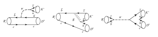
Figure 1: Diagrams for $B^{+}_{c}\rightarrow D^{0}K^{+}$ decay.

According to the QCD factorization, the amplitude of $B^{+}_{c}\rightarrow D^{0}K^{+}$ decay is given by

$$M_{QCDF}(B^{+}_{c}\rightarrow D^{0}K^{+})=\frac{G_{F}}{\sqrt{2}}f_{K^{+}}\Big{[} (m_{B^{+}_{c}}^{2}-m_{D^{0}}^{2})F^{B^{+}_{c}\rightarrow D^{0}}(m_{K^{+}}^{2})(a_{1}V^{*}_{ub}V{us}+a_{4}V^{*}_{tb}V_{ts})$$ (5)

$$+f_{B^{+}_{c}}f_{D^{0}}b_{2}V^{*}_{cb}V_{cs}\Big{]},$$

where $a_{1}$ and $a_{4}$ correspond to the current-current tree and penguin, and $b_{2}$ corresponds to the current-current annihilation coefficients that are given by

$$a_{1} = c_{1}+\frac{c_{2}}{N_{c}},\quad a_{4}=c_{4}+\frac{c_{3}}{N_{c}},$$

$$b_{2} = \frac{C_{F}}{N_{c}^{2}}c_{2}A_{1}^{i},$$ (6)

$c_{i}$ are the Wilson coefficients, $N_{c}=3$ is the color number and

$$A_{1}^{i} = 2\pi\alpha_{s}[9(X_{A}-4+\frac{\pi^{2}}{3})+r_{\chi}^{D^{0}}r_{\chi}^{K^{+}}X_{A}^{2}],$$

$$C_{F} = \frac{N_{c}^{2}-1}{2N_{c}},$$ (7)

where $r_{\chi}^{D^{0}}=1.85$ and $r_{\chi}^{K^{+}}1.14$. For the running coupling constant, at two loop order (NLO) the solution of the renormalizaton group equation can always be written in the form

$$\alpha_{s}(\mu)=\frac{4\pi}{\beta_{0}ln\frac{\mu^{2}}{\Lambda_{QCD}^{2}}}[1-\frac{\beta_{1}}{\beta_{0}^{2}}\frac{ln(ln\frac{\mu^{2}}{\Lambda_{QCD}^{2}})}{ln\frac{\mu^{2}}{\Lambda_{QCD}^{2}}}],$$ (8)

here

$$\beta_{0}=\frac{11N_{c}-2n_{f}}{3},\;\beta_{1}=\frac{34N_{c}^{2}}{3}-\frac{10N_{c}n_{f}}{3}-2C_{F}n_{f},$$ (9)

and running $\alpha_{s}(\mu)$ evaluated with $n_{f}=5$. There are large theoretical uncertainties related to the modeling of power corrections corresponding to weak annihilation effects, we parameterize these effects in terms of the divergent integrals $X_{A}$ (weak annihilation)

$$X_{A}=(1+\rho e^{i\phi})\ln{\frac{m_{B^{+}_{c}}}{\Lambda_{h}}},$$ (10)

where, can be obtained by using $\rho=0.5$, $\phi=-55^{\circ}$ and $\Lambda_{h}=0.5Gev$.

2.2 Decay amplitudes of intermediate states

Each decay in the intermediate states is a two body decay of $B^{+}_{c}$ meson that until now the amplitude of such decays has been achieved in many ways: naive factorization, QCD factorization, improved factorization and using QCD perturbation. In present section, we use QCD factorization to obtain intermediate state amplitudes.
The first intermediate state decay is: $B^{+}_{c}\rightarrow J/\psi D^{+(*)}_{s}$. Usually, in FSI, the dominant contribution of intermediate amplitudes is considered, however, here we consider all of them. The decay $B^{+}_{c}\rightarrow J/\psi D^{+}_{s}$ happens both through $\bar{b}\rightarrow\bar{c}$ and $\bar{b}\rightarrow\bar{s}$ transitions. The tree transition of $\bar{b}\rightarrow\bar{c}$ concludes two contributions of Wilson’s coefficients: $a_{1}$ and $a_{2}$. The matrix elements of both contributions are $V_{cb}^{*}V_{cs}$. For $a_{1}$ contribution, the mesons of $J/\psi$ and $D^{+}_{s}$ place in form factor and decay constant, respectively. But, in $a_{2}$ contribution, conversely.
The penguin transition $\bar{b}\rightarrow\bar{s}$ has $a_{3}$ and $a_{4}$ Wilson contributions. In $a_{3}$ contribution, mesons of $D^{+}_{s}$ and $J/\psi$ place in the form factor and decay constant, respectively. But, in the $a_{4}$ coefficient the rule is the opposite of this. Corresponded matrix elements are $V_{tb}^{*}V_{ts}$.
The second and third intermediate state decays are $B^{+}_{c}\rightarrow D^{+(*)}_{s}\phi$ and $B^{+}_{c}\rightarrow D^{+(*)}K^{0(*)}$. These decays only have penguin transition. In fact, they have just $a_{4}$ contribution in which mesons of $D^{+}_{s}$ and $D^{+}$ place in form factor and mesons of $\phi$ and $K^{0}$ place in decay constant. Their CKM matrix elements are $V_{tb}^{*}V_{ts}$.
The fourth and fifth intermediate state decays are the decays of $B^{+}_{c}\rightarrow D^{+(*)}_{s}P$ with $P=\pi^{0},\rho^{0},\omega,\eta$ which include the $a_{2}$ and $a_{3}$ contributions of tree transition $\bar{b}\rightarrow\bar{u}$ and penguin transition $\bar{b}\rightarrow\bar{s}$, respectively. The corresponding matrix elements are $V_{ub}^{*}V_{us}$ and $V_{tb}^{*}V_{ts}$, respectively. The appearance of the five decays mentioned above can be seen in the Fig. 2.

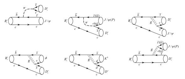
Figure 2: Feynman diagrams for intermediate states decays.

In all these decays, there were contributions of Wilson. These contributions are derived from the combination of Wilson coefficients. If these coefficients are used in the normal from, the factorization is called naive factorization, while, using Wilson effective coefficients, it is called QCD factorization. Wilson tree and penguin contributions get from $a_{1,2}=c_{1,2}+c_{2,1}/3$ and $a_{3,4}=c_{3,4}+c_{4,3}/3$, respectively. The $c_{i}$ are normal Wilson coefficients, these become Wilson effective coefficients if the vertex correction and hard gluon scattering are taken into account ($c_{i}\rightarrow c_{i}^{eff}$). In all of these decays, we used terms like: tree transition, penguin transition, decay constant and form factor. The form factors and decay constants for pseudo scalar and vector mesons can be written respectively as [13]:

$$\langle P(p^{\prime})|V_{\mu}|B(p)\rangle = [(p+p^{\prime})_{\mu}-\frac{m_{B}^{2}-m_{P}^{2}}{q^{2}}q_{\mu}]F_{1}(q^{2})+\frac{m_{B}^{2}-m_{P}^{2}}{q^{2}}q_{\mu}F_{0}(q^{2})$$

$$\langle 0|A_{\mu}|P(q)\rangle = if_{p}q_{\mu}$$

$$\langle V(\epsilon,p^{\prime})|V_{\mu}-A_{\mu}|B(p)\rangle = (\epsilon^{*}\cdot q)\frac{2m_{V}}{q^{2}}q_{\mu}A_{0}(q^{2})+(m_{B}+m_{V})[\epsilon^{*}_{\mu}-\frac{\epsilon^{*}\cdot q}{q^{2}}q_{\mu}]A_{1}(q^{2})$$

$$-\frac{\epsilon^{*}\cdot q}{m_{B}+m_{V}}[(p+p^{\prime})_{\mu}-\frac{m_{B}^{2}-m_{V}^{2}}{q^{2}}q_{\mu}]A_{2}(q^{2})$$

$$\langle 0|V_{\mu}|V(\epsilon,q)\rangle = if_{V}m_{V}\epsilon_{\mu},$$ (11)

where p and v are pseudo scalar and vector mesons, respectively. The q parameter is the four-momentum of propagator the square of which is $q^{2}=m_{B}^{2}+m_{p}^{2}-2m_{B}p^{0}_{p}$. So, amplitudes of intermediate decays take the following form:

$$M(B^{+}_{c}\rightarrow J/\psi D^{+}_{s}) = i\sqrt{2}G_{F}m_{J/\psi}(\epsilon_{J/\psi}\cdot p_{B})\{[a_{1}f_{D^{+}_{s}}A_{0}^{B^{+}_{c}\rightarrow J/\psi}(m^{2}_{D^{+}_{s}})+a_{2}f_{J/\psi}F_{1}^{B^{+}_{c}\rightarrow D^{+}_{s}}(m^{2}_{J/\psi})]$$

$$\times V^{*}_{cb}V_{cs}+[a_{3}f_{J/\psi}F_{1}^{B^{+}_{c}\rightarrow D^{+}_{s}}(m^{2}_{J/\psi})+a_{4}f_{D^{+}_{s}}A_{0}^{B^{+}_{c}\rightarrow J/\psi}(m^{2}_{D^{+}_{s}})]V^{*}_{tb}V_{ts}\}$$

$$M(B^{+}_{c}\rightarrow J/\psi D^{*+}_{s}) = i\frac{G_{F}}{\sqrt{2}}\{f_{D^{*+}_{s}}m_{D^{*+}_{s}}[(\epsilon_{J/\psi}\cdot\epsilon_{D^{*+}_{s}})(m_{B^{+}_{c}}+m_{J/\psi})A_{1}^{B^{+}_{c}\rightarrow J/\psi}(m^{2}_{D^{*+}_{s}})$$

$$-(\epsilon_{J/\psi}\cdot p_{B^{+}_{c}})(\epsilon_{D^{*+}_{s}}\cdot p_{B^{+}_{c}})\frac{2A_{2}^{B^{+}_{c}\rightarrow J/\psi}(m^{2}_{D^{*+}_{s}})}{m_{B^{+}_{c}}+m_{J/\psi}}](a_{1}V^{*}_{cb}V_{cs}+a_{4}V^{*}_{tb}V_{ts})$$

$$+f_{J/\psi}m_{J/\psi}[(\epsilon_{J/\psi}\cdot\epsilon_{D^{*+}_{s}})(m_{B^{+}_{c}}+m_{D^{*+}_{s}})A_{1}^{B^{+}_{c}\rightarrow D^{*+}_{s}}(m^{2}_{J/\psi})$$

$$-(\epsilon_{J/\psi}\cdot p_{B^{+}_{c}})(\epsilon_{D^{*+}_{s}}\cdot p_{B^{+}_{c}})\frac{2A_{2}^{B^{+}_{c}\rightarrow D^{*+}_{s}}(m^{2}_{J/\psi})}{m_{B^{+}_{c}}+m_{D^{*+}_{s}}}]a_{2}V^{*}_{cb}V_{cs}\}$$

$$M(B^{+}_{c}\rightarrow D^{*+}_{s}\phi) = i\frac{G_{F}}{\sqrt{2}}[(\epsilon_{D^{*+}_{s}}\cdot\epsilon_{\phi})(m_{B^{+}_{c}}+m_{D^{*+}_{s}})A_{1}^{B^{+}_{c}\rightarrow D^{*+}_{s}}(m^{2}_{\phi})$$

$$-(\epsilon_{\phi}\cdot p_{B^{+}_{c}})(\epsilon_{D^{*+}_{s}}\cdot p_{B^{+}_{c}})\frac{2A_{2}^{B^{+}_{c}\rightarrow D^{*+}_{s}}(m^{2}_{\phi})}{m_{B^{+}_{c}}+m_{D^{*+}_{s}}}]a_{4}V^{*}_{tb}V_{ts}$$

$$M(B^{+}_{c}\rightarrow D^{+}_{s}\phi) = i\sqrt{2}G_{F}f_{\phi}m_{\phi}(\epsilon_{\phi}\cdot p_{B})F_{1}^{B^{+}_{c}\rightarrow D^{+}_{s}}(m^{2}_{\phi})a_{4}V^{*}_{tb}V_{ts}$$

$$M(B^{+}_{c}\rightarrow D^{+}K^{0}) = i\frac{G_{F}}{\sqrt{2}}f_{K^{0}}(m^{2}_{B^{+}_{c}}-m^{2}_{D^{+}})F^{B^{+}_{c}\rightarrow D^{+}}(m^{2}_{K^{0}})a_{4}V^{*}_{tb}V_{ts}$$

$$M(B^{+}_{c}\rightarrow D^{+}_{s}P) = i\frac{G_{F}}{\sqrt{2}}f_{P}(m^{2}_{B^{+}_{c}}-m^{2}_{D^{+}_{s}})F^{B^{+}_{c}\rightarrow D^{+}_{s}}(m^{2}_{P})(a_{2}V^{*}_{ub}V_{us}+a_{3}V^{*}_{tb}V_{ts}),$$ (12)

with $P=\pi^{0},\rho^{0},\omega,\eta$; $a_{2}=c_{2}+c_{1}/3$ and $a_{3}=c_{3}+c_{4}/3$.

3 Amplitudes of the long distance processes

We know the above mentioned decays as intermediate state decays. In this process, first the decaying meson decays into two intermediate mesons, then, these two intermediate mesons are changed into final mesons by exchanging a meson. FSI is done using two channels named T-channel and cross section-channel. In T-channel, the two final mesons share co-flavour quark and anti-quark with their same flavour. But, in cross section channel, two final mesons exchange two non-flavoured quarks or anti-quarks, crosswisely. As we know, the $D^{0}$ and $K^{+}$ mesons constructed from $c\bar{u}$ and $u\bar{s}$ quark anti-quark, respectively. Then, these two mesons, which are in the final state, can share quark anti-quark with their same flavour i.e. u quark in channel T. On the other hand, intermediate state mesons can be produced by sharing co-flavoured quark anti-quark like c, s and d which can be $J/\psi D_{s}^{+(*)}$, $D_{s}^{+(*)}\phi$ and $D^{+(*)}K^{0(*)}$ mesons. Interchanging mesons of these processes are called $D^{0}$, $K^{-}$ and $\pi^{-}$, respectively. In cross section channel, two final state mesons $D^{0}$ and $K^{+}$ exchange $\bar{u}$ and $\bar{s}$ anti-quarks, respectively. In this state, $D^{+}_{s}P$ with $P=\omega$, $\rho^{0}$, $\eta$ and $\pi^{0}$ are intermediate mesons and $K^{-}$ is interchange meson. In this channel, there is another state in which two final mesons $D^{0}$ and $K^{+}$ mesons exchange c and u quarks, respectively. Thus, intermediate mesons are the same as the previous i.e. $D^{+}_{s}p$ and $D^{0}$ is the intermediate meson. Fig. 3

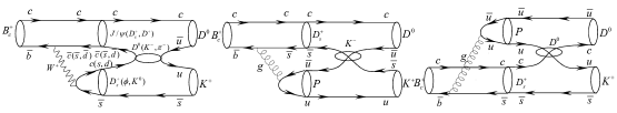
Figure 3: Diagrams of meson vertexes.

illustrates FSI diagrams for $B^{+}_{c}\rightarrow D^{0}K^{+}$ decay through T and cross section channels. The form factors corresponded to FSI are different from those defined in the previous section. In the two-body decay of previous section the exchanged particle in interaction i.e. propagator is the elementary particle boson or gluon, but in FSI the exchange particle is a meson. Since, the form factor depends on mass and momentum of particle, here too, we introduce the FSI form factor as a function of mass and momentum $F(q^{2},m_{i}^{2})=(\Lambda^{2}-m_{i}^{2})/(\Lambda^{2}-q^{2})$ in which $m_{i}$ and q are the mass and momentum parameter that shows the effectiveness of strong interaction in a weak interaction through $\Lambda=m_{i}+\eta\Lambda_{QCD}$. The parameter $\Lambda_{QCD}$ is strong interaction energy scale which has the range of from 225 MeV to 750 MeV. We usually consider the value of $\Lambda_{QCD}$ constant equal to 225 MeV. Then, we change the phenomenological parameter $\eta$. The range of this parameter is defined according to the exchanged mesons. In Ref. [15], D and $D^{*}$ are exchanged mesons which the authors have considered the range of $\eta$ parameter from 0.5 to 3. However, in Ref [16], for similar exchanged mesons, authors have considered 5 for parameter $\eta$. In Ref [17], calculations are made for $\eta=4$. In present paper, we have considered the range of $\eta$ from 1 to 3. The more the value of $\eta$, the more the effect of strong interaction. The mesons vertex factor is another important factor in FSI. This factor is proportional to the coupling constant of meson in vertices. There are three mesons in the top vertex and three mesons in the down vertex which should follow meson vertex rules. The first of them says that there must be at least one vector meson in each vertex. Also, vector mesons should be symmetric in the final and intermediate state in the manner that if two final mesons are pseudo scalar, the intermediate mesons both should either be pseudo scalar or vector mesons. In the decay considered in this article, $B^{+}_{c}\rightarrow D^{0}K^{+}$, because two final mesons are pseudo scalar, the intermediate mesons both should be either pseudo scalar or vector mesons. In the case in which both intermediate mesons are pseudo scalar, the exchanged meson should be vector meson. In the case in which both intermediate mesons are vector , the intermediate mesons can be both scalar and vector. Applying these rules, the following decays in the T-channel can be calculated:

$$B^{+}_{c} \rightarrow J/\psi D^{*+}_{s}\rightarrow D^{0}K^{+}\;\;\rm{exchang\;mesons\;are}\;D^{0},D^{*0}$$

$$B^{+}_{c} \rightarrow D^{+}K^{0}\rightarrow D^{0}K^{+}\;\;\rm{exchang\;meson\;is}\;\rho^{-}$$

$$B^{+}_{c} \rightarrow D^{*+}K^{*0}\rightarrow D^{0}K^{+}\;\;\rm{exchang\;mesons\;are}\;\pi^{-},\rho^{-}$$

$$B^{+}_{c} \rightarrow D^{*+}_{s}\phi\rightarrow D^{0}K^{+}\;\;\rm{exchang\;mesons\;are}\;K^{-},K^{*-}.$$ (13)

Also in the cross section channel the following decays are calculated:

$$B^{+}_{c} \rightarrow D^{+}_{s}\pi^{0}\rightarrow D^{0}K^{+}\;\;\rm{exchang\;meson\;is}\;D^{*0}$$

$$B^{+}_{c} \rightarrow D^{+}_{s}\eta\rightarrow D^{0}K^{+}\;\;\rm{exchang\;meson\;is}\;D^{*0}$$

$$B^{+}_{c} \rightarrow D^{*+}_{s}\rho^{0}\rightarrow D^{0}K^{+}\;\;\rm{exchang\;mesons\;are}\;D^{0},D^{*0}$$

$$B^{+}_{c} \rightarrow D^{*+}_{s}\omega\rightarrow D^{0}K^{+}\;\;\rm{exchang\;mesons\;are}\;D^{0},D^{*0}$$

$$B^{+}_{c} \rightarrow D^{+}_{s}\pi^{0}\rightarrow D^{0}K^{+}\;\;\rm{exchang\;meson\;is}\;K^{*-}$$

$$B^{+}_{c} \rightarrow D^{+}_{s}\eta\rightarrow D^{0}K^{+}\;\;\rm{exchang\;meson\;is}\;K^{*-}$$

$$B^{+}_{c} \rightarrow D^{*+}_{s}\rho^{0}\rightarrow D^{0}K^{+}\;\;\rm{exchang\;mesons\;are}\;K^{-},K^{*-}$$

$$B^{+}_{c} \rightarrow D^{*+}_{s}\omega\rightarrow D^{0}K^{+}\;\;\rm{exchang\;mesons\;are}\;K^{-},K^{*-}.$$ (14)

The meson vertices corresponded to FSI are seen in the Fig. 4.

Figure 4: Diagrams of meson vertexes.

For example, consider to the meson vertex $\phi KK$. This vertex shows the decay of $\phi$ meson into two KK mesons. The coupling constant of the vertex is obtained from the relation $g_{\phi KK}=(m_{\phi}/|\overrightarrow{p}_{K}|)\sqrt{(6\pi\Gamma^{exp}_{\phi\rightarrow KK})/|\overrightarrow{p}_{K}|}$ in which in the particles data group (PDG), $\Gamma^{exp}_{\phi\rightarrow KK}$ is given 2.09 MeV [9]. The parameter $|\vec{p}|$ is the K-meson’s momentum in the $\phi$-meson’s rest frame. The rest of the coupling constant of their meson vertices, can be obtained from the similar relation for $\phi$-meson decay. The vertex factors which include a vector meson V and two pseudo scalar mesons P, can be obtained from $\langle P_{1}(p_{1})P_{2}(p_{2})|i\ell|V_{3}(\epsilon_{3},p_{3})\rangle=-ig_{p_{1}p_{2}V}\epsilon_{3}\cdot(p_{1}+p_{2})$. As an example, vertex factor of $J/\psi DD$ and $\phi KK$ are:

$$\langle D(p_{1})D(p_{2})|i\ell|J/\psi(\epsilon_{3},p_{3})\rangle = -ig_{J/\psi DD}\epsilon_{3}\cdot(p_{1}+p_{2}),$$

$$\langle K(p_{1})K(p_{2})|i\ell|\phi(\epsilon_{3},p_{3})\rangle = -ig_{\phi KK}\epsilon_{3}\cdot(p_{1}+p_{2}).$$ (15)

The factor of the $\langle P_{1}(p_{1})V_{2}(\epsilon_{2},p_{2})|i\ell|V_{3}(\epsilon_{3},p_{3})\rangle=-i\sqrt{2}g_{p_{1}V_{2}V_{3}}\epsilon_{\mu\nu\alpha\beta}\epsilon_{2}^{\mu}\epsilon_{3}^{*\nu}p_{1}^{\alpha}p_{2}^{\beta}$ is used for the vertex factors which include a pseudo scalar meson P and two vector mesons V, so, the vertex factor of $J/\psi D^{*}D$ and $\phi K^{*}K$ are:

$$\langle D(p_{1})D^{*}(\epsilon_{2},p_{2})|i\ell|J/\psi(\epsilon_{3},p_{3})\rangle = -i\sqrt{2}g_{J/\psi D^{*}D}\epsilon_{\mu\nu\alpha\beta}\epsilon_{2}^{\mu}\epsilon_{3}^{*\nu}p_{1}^{\alpha}p_{2}^{\beta}$$

$$\langle K(p_{1})K^{*}(\epsilon_{2},p_{2})|i\ell|\phi(\epsilon_{3},p_{3})\rangle = -i\sqrt{2}g_{\phi K^{*}K}\epsilon_{\mu\nu\alpha\beta}\epsilon_{2}^{\mu}\epsilon_{3}^{*\nu}p_{1}^{\alpha}p_{2}^{\beta}.$$ (16)

Finally, one can calculate the amplitude of graphs that have meson loops as shown in Fig. 4, for the case in which both mesons are pseudo scalar as:

$$M(B^{+}_{c}(p_{B^{+}_{c}}) \rightarrow P_{1}(p_{1})P_{2}(p_{2})\rightarrow P_{3}(p_{3})P_{4}(p_{4}))=\frac{1}{2}\int\frac{d^{3}\overrightarrow{p_{1}}}{2E_{1}(2\pi)^{3}}\frac{d^{3}\overrightarrow{p_{2}}}{2E_{2}(2\pi)^{3}}$$ (17)

$$\times(2\pi)^{4}\delta^{4}(p_{B^{+}_{c}}-p_{1}-p_{2})M(B^{+}_{c}\rightarrow P_{1}P_{2})G(P_{1}P_{2}\rightarrow P_{3}P_{4}),$$

in Eq. (17), $P_{1}P_{2}$ and $P_{3}P_{4}$ mesons are intermediate and final state mesons, respectively and $G(P_{1}P_{2}\rightarrow P_{3}P_{4})$ shows meson vortices factors which include the product of top factor in down factor in each graph. For the case which both intermediate mesons are vector mesons, the amplitude of graph, including meson loop is obtained from the following equation:

$$M(B^{+}_{c}(p_{B^{+}_{c}}) \rightarrow V_{1}(\epsilon_{1},p_{1})V_{2}(\epsilon_{2},p_{2})\rightarrow P_{3}(p_{3})P_{4}(p_{4}))=\frac{1}{2}\int\frac{d^{3}\overrightarrow{p_{1}}}{2E_{1}(2\pi)^{3}}\frac{d^{3}\overrightarrow{p_{2}}}{2E_{2}(2\pi)^{3}}$$ (18)

$$\times(2\pi)^{4}\delta^{4}(p_{B^{+}_{c}}-p_{1}-p_{2})f_{V_{1}}m_{V_{1}}V_{CKM}[(\epsilon_{1}^{*}\cdot\epsilon_{2}^{*})(m_{B^{+}_{c}}+m_{2})A_{1}^{B^{+}_{c}\rightarrow V_{2}}(m_{1}^{2})$$

$$-(\epsilon^{*}_{1}\cdot p_{B^{+}_{c}})(\epsilon^{*}_{2}\cdot p_{B^{+}_{c}})\frac{2A_{2}^{B^{+}_{c}\rightarrow V_{2}}(m_{1}^{2})}{m_{B^{+}_{c}}+m_{2}}]G(P_{1}P_{2}\rightarrow P_{3}P_{4}),$$

which is assumed in that the vector mesons $V_{2}$ and $V_{1}$ are set in form factor and vacuum state, respectively. But, in the case with vector mesons $V_{1}$ and $V_{2}$ are setted in form factor and vacuum state, respectively, indices are replaced in Eq. (18). So, the first amplitude of the nineteen amplitudes of Fig. 4. i.e amplitude $B^{+}_{c}\rightarrow D^{0}K^{+}$, with $D^{0}(q)$ as an exchanged meson, can be written as:

$$M(3a,D^{0}) = i\frac{G_{F}}{4\sqrt{2}\pi m_{B^{+}_{c}}}f_{D^{*+}_{s}}m_{D^{*+}_{s}}a_{1}V^{*}_{cb}V_{cs}g_{J/\psi DD}g_{D_{s}^{*}DK}\int^{+1}_{-1}|\overrightarrow{p}_{1}|d(cos\theta)\frac{F^{2}(q^{2},m_{D}^{2})}{q^{2}-m_{D}^{2}}$$ (19)

$$\times[(m_{B^{+}_{c}}+m_{J/\psi})A_{1}^{B^{+}_{c}\rightarrow J/\psi}(m^{2}_{D^{*+}_{s}})K_{1}-\frac{2A_{2}^{B^{+}_{c}\rightarrow J/\psi}(m^{2}_{D^{*+}_{s}})}{m_{B^{+}_{c}}+m_{J/\psi}}K^{\prime}_{1}],$$

in Eq. (19) $\theta$ is the angle between momentums $\overrightarrow{p}_{1}$ and $\overrightarrow{p}_{3}$, also $q=p_{1}-p_{3}=p_{4}-p_{2}$ is the momentum of exchanged meson. In this case, $q^{2}-m_{D}^{2}$ has the form $m_{1}^{2}-2E_{1}E_{3}+2|\overrightarrow{p}_{1}||\overrightarrow{p}_{3}|cos\theta$. The parameters $K_{1}$ and $K^{\prime}_{1}$ show the product of polarization vectors of vector mesons where $K_{1}=(\epsilon_{1}\cdot p_{3})(\epsilon_{2}\cdot p_{4})(\epsilon^{*}_{1}\cdot\epsilon_{2}^{*})$ and $K^{\prime}_{1}=(\epsilon_{1}\cdot p_{3})(\epsilon_{2}\cdot p_{4})(\epsilon_{1}\cdot p_{2})(\epsilon_{2}\cdot p_{1})$. The second amplitude shows the same process as before with the difference that the exchanged meson in this case is vector meson, so, we have:

$$M(3a,D^{*0}) = i\frac{G_{F}}{8\sqrt{2}\pi m_{B^{+}_{c}}}f_{D^{*+}_{s}}m_{D^{*+}_{s}}a_{1}V^{*}_{cb}V_{cs}g_{J/\psi D^{*}D}g_{D_{s}^{*}D^{*}K}\int^{+1}_{-1}|\overrightarrow{p}_{1}|d(cos\theta)\frac{F^{2}(q^{2},m_{D^{*}}^{2})}{q^{2}-m_{D^{*}}^{2}}$$ (20)

$$\times[(m_{B^{+}_{c}}+m_{J/\psi})A_{1}^{B^{+}_{c}\rightarrow J/\psi}(m^{2}_{D^{*+}_{s}})K_{2}-\frac{2A_{2}^{B^{+}_{c}\rightarrow J/\psi}(m^{2}_{D^{*+}_{s}})}{m_{B^{+}_{c}}+m_{J/\psi}}K^{\prime}_{2}],$$

where $K_{2}=\epsilon_{\mu\nu\alpha\beta}\epsilon_{1}^{\mu}\epsilon_{D^{*}}^{\nu}p_{3}^{\alpha}p_{1}^{\beta}\epsilon_{\rho\sigma\lambda\eta}\epsilon_{2}^{\rho}\epsilon_{D^{*}}^{\sigma}p_{4}^{\lambda}p_{2}^{\eta}(\epsilon_{1}^{*}\cdot\epsilon_{2}^{*})$ and $K^{\prime}_{2}=\epsilon_{\mu\nu\alpha\beta}\epsilon_{1}^{\mu}\epsilon_{D^{*}}^{\nu}p_{3}^{\alpha}p_{1}^{\beta}\epsilon_{\rho\sigma\lambda\eta}\epsilon_{2}^{\rho}\epsilon_{D^{*}}^{\sigma}p_{4}^{\lambda}p_{2}^{\eta}(\epsilon_{1}\cdot p_{B_{c}})(\epsilon_{2}\cdot p_{B_{c}})$. In this amplitude, $q^{2}-m_{D^{*}}^{2}$ has the form of $m_{1}^{2}+m_{3}^{2}-m_{D^{*}}^{2}-2E_{1}E_{3}+2|\overrightarrow{p}_{1}||\overrightarrow{p}_{3}|cos\theta$.

$$M(3b,K^{-}) = i\frac{G_{F}}{4\sqrt{2}\pi m_{B^{+}_{c}}}f_{\phi}m_{\phi}a_{4}V^{*}_{tb}V_{ts}g_{D^{*}_{s}DK}g_{\phi KK}\int^{+1}_{-1}|\overrightarrow{p}_{1}|d(cos\theta)\frac{F^{2}(q^{2},m_{K}^{2})}{q^{2}-m_{K}^{2}}$$ (21)

$$\times[(m_{B^{+}_{c}}+m_{D^{*+}_{s}})A_{1}^{B^{+}_{c}\rightarrow D^{*+}_{s}}(m^{2}_{\phi})K_{1}-\frac{2A_{2}^{B^{+}_{c}\rightarrow D^{*+}_{s}}(m^{2}_{\phi})}{m_{B^{+}_{c}}+m_{D^{*+}_{s}}}K^{\prime}_{1}].$$

To calculate the amplitude $M(3b,K^{*-})$ it is enough to do as follow:
1) convert 4 to 8 in the denominator of the first fraction line,
2) replace $g_{D^{*}_{s}DK}g_{KK\phi}$ with $g_{D^{*}_{s}DK^{*}}g_{KK^{*}\phi}$,
3) replace $m_{K}$ with $m_{K^{*}}$ in the face and denominator of the second fraction line,
4) convert coefficients $K_{1}$ and $K^{\prime}_{1}$ to $K_{2}$ and $K^{\prime}_{2}$, respectively.
The FSI amplitude of the third graph of figure 3, the amplitude $B^{+}_{c}\rightarrow D^{+}(p_{1})K^{0}(p_{2})\rightarrow D^{0}(p_{3})K^{+}(p_{4})$ with $\rho^{-}(q)$ as exchange meson can be written as:

$$M(3c) = -g_{DD\rho}g_{KK\rho}\int^{+1}_{-1}\frac{|\overrightarrow{p}_{1}|d(cos\theta)}{16\pi m_{B^{+}_{c}}}M(B^{+}_{c}\rightarrow D^{+}K^{0})\frac{F^{2}(q^{2},m_{\rho}^{2})}{q^{2}-m_{\rho}^{2}}K_{3},$$ (22)

where $K_{3}=p_{1\mu}\epsilon_{\rho}^{\mu}p_{2\nu}\epsilon_{\rho}^{\nu}$. The amplitude of the remaining graphs of figure 3 are obtained as written amplitudes. Finally, the total amplitude of the FSI for $B^{+}_{c}\rightarrow D^{0}K^{+}$ decay is calculated as:

$$M_{FSI}(B^{+}_{c}\rightarrow D^{0}K^{+}) = M(3a,D)+M(3a,D^{*})+M(3b,K)+M(3b,K^{*})$$ (23)

$$+M(3c)+M(3d,\pi)+M(3d,\rho)\ldots M(3l,K)+M(3l,K^{*}).$$

At the end, one can calculate the branching ratio as:

$$\mathcal{B}(B^{+}_{c}\rightarrow D^{0}K^{+}) = \frac{1}{\Gamma_{{\rm{tot}}}}\frac{|M(B^{+}_{c}\rightarrow D^{0}K^{+})|^{2}}{16\pi m_{B^{+}_{c}}},$$ (24)

where $\Gamma_{\rm{tot}}=4.219\times 10^{-13}$ GeV [18].

4 Experimental and theoretical dada

The meson masses and decay constants needed in our calculations are listed in the section (I) of the table 1. The Cabibbo-Kobayashi-Maskawa (CKM) matrix is a $3\times 3$ unitary matrix, the elements of this matrix can be parameterized by three mixing angles $A$, $\lambda$, $\rho$ and a CP-violating phase $\eta$ [9]: $V_{us}=\lambda$, $V_{ub}=A\lambda^{3}(\rho-i\eta)$, $V_{cs}=1-\lambda^{2}/2$, $V_{cb}=A\lambda^{2}$, $V_{ts}=-A\lambda^{2}$ and $V_{tb}=1$, the results are shown in section (II) of the table 1. The values of the coupling constants and the corresponding form factors are given in sections (III) and (IV) of the table 1, respectively. The Wilson coefficients $c_{1}$, $c_{2}$, $c_{3}$ and $c_{4}$ in the effective weak Hamiltonian have been reliably evaluated by the next-to-leading logarithmic order. To proceed, we use the following numerical values at $\mu=m_{b}$ scale, which have been obtained in the NDR scheme, these coefficient numbers are inserted in the section (V) of the table 1 [14].

Table 1: Input parameters.

I) Mesons masses
decay constants
(in units of MeV) [9]
$m_{B^{+}_{c}}=6274.9\pm 0.08$	$m_{J/\psi}=3096.900\pm 0.006$	$m_{D^{+*}_{s}}=2112.2\pm 0.4$
$m_{D^{+}_{s}}=1968.34\pm 0.07$	$m_{D^{0}}=1864.83\pm 0.05$	$m_{\phi}=1019.461\pm 0.016$
$m_{\omega}=782.65\pm 0.12$	$m_{\rho^{0}}=775.26\pm 0.25$	$m_{\eta}=547.862\pm 0.017$
$m_{K^{0}}=497.611\pm 0.013$	$m_{K^{+}}=493.677\pm 0.016$	$m_{\pi^{0}}=134.9773\pm 0.0005$
$f_{B_{c}}=489\pm 4$	$f_{J/\psi}=418\pm 9$	$f_{D^{*}_{s}}=315\pm 8$
$f_{D_{s}}=294\pm 7$	$f_{D}=234\pm 15$	$f_{\phi}=215\pm 5$
$f_{\rho}=210\pm 4$	$f_{\omega}=195\pm 2$	$f_{K}=159.8\pm 1.84$
$f_{\pi}=130.70\pm 0.46$	$f_{\eta}=63.6\pm 0.23$
II) CKM matrix elements [9]
$V_{ub}=0.00394\pm 0.00036$	$V_{cb}=0.0422\pm 0.0008$	$V_{tb}=1.019\pm 0.025$
$V_{us}=0.2243\pm 0.0005$	$V_{cs}=0.997\pm 0.017$	$V_{ts}=0.0394\pm 0.0023$
III) Coupling constants
$g_{DD\rho}=2.52$	$g_{D^{*}D\rho}=2.82$	$g_{J/\psi DD}=7.71$
$g_{J/\psi D^{*}D}=8.64$ [19]	$g_{D^{*}D\pi}=12.5$ [20]	$g_{D^{*}_{s}DK}=18.34$ [21]
$g_{D^{*}_{s}D^{*}K}=9.23$	$g_{K^{*}K\pi}=4.6$ [22]
$g_{K^{*}K\rho}=g_{K^{*}K\phi}=6.48$	$g_{KK\rho}=g_{KK\phi}=5.55$ [23]
IV) Form factors [24]
$A_{0}^{B_{c}\rightarrow J/\psi}=0.58^{+0.01}_{-0.03}$	$A_{1}^{B_{c}\rightarrow J/\psi}=0.63^{+0.03}_{-0.03}$	$A_{2}^{B_{c}\rightarrow J/\psi}=0.74^{+0.05}_{-0.06}$
$A_{1}^{B_{c}\rightarrow D^{+*}_{s}}=0.18^{+0.01}_{-0.02}$	$A_{2}^{B_{c}\rightarrow D^{+*}_{s}}=0.20^{+0.02}_{-0.03}$
$F^{B_{c}\rightarrow D}=0.057^{+0.06}_{-0.08}$	$F^{B_{c}\rightarrow D_{s}}=0.15\pm 0.01$
V) Wilson coefficients [14]
$c_{1}=1.081$	$c_{2}=-0.190$	$c_{3}=0.014$
$c_{4}=-0.036$

Using the parameters relevant for the $B^{+}_{c}\rightarrow D^{0}K^{+}$ decay, we get flavor averaged branching ratio for the QCD factorization method as:

$$\mathcal{B}_{QCDF}(B^{+}_{c}\rightarrow D^{0}K^{+})=1.41\times 10^{-7}.$$ (25)

Now, applying the effects of the FSI, we obtain the branching ratios of $B^{+}_{c}\rightarrow D^{0}K^{+}$ decay with different values of $\eta$, for $\eta=1$ we get the number of the $(1.17\pm 0.19)\times 10^{-5}$, for $\eta=2$ the value is $(5.89\pm 0.92)\times 10^{-5}$ and the result of our calculation is $(11.65\pm 1.73)\times 10^{-5}$ by choosing $\eta=3$. The results show that the branching ratios are very sensitive to the variation of $\eta$.

5 Conclusion

The decay of $B^{+}_{c}\rightarrow D^{0}K^{+}$ was calculated theoretically before being experimentally observed and before any experimented data is measured for it. The result was $1.34\times 10^{-7}$ using QCD factorization approach and $6.60\times 10^{-5}$ using perturbative QCD method. Until the LHCb collaboration obtained the experimental branching ratio of this decay between $3.72\times 10^{-5}$ and $11.16\times 10^{-5}$. In this work, we have calculated the contribution of the FSI, i.e. inelastic rescattering processes to the branching ratio of $B^{+}_{c}\rightarrow D^{0}K^{+}$ decay and find that it spans a relatively wider range of $(1.17\sim 11.65)\times 10^{-5}$ which is obviously larger than the theoretically predicted value and comparable with the perturbative QCD prediction. Our predicted also covers the experimental range.

References

- [1] F. Abe et al., CDF Collaboration, Phys. Rev. Lett 81 (1998) 2432.
- [2] T. Aaltonen et al., CDF Collaboration, Phys. Rev. Lett 100 (2008) 182002.
- [3] V. Abazov et al., Collaboration, Phys. Rev. Lett 101 (2008) 012001.
- [4] J. Zhang and X.Q. Yu, Eur. Phys. J. C 63 (2009) 435.
- [5] H.f. Fu, Y. Jiang, C.S. Kim and G.L. Wang, JHEP 1106 (2011) 015.
- [6] R. Aaij et al., LHCb Collaboration, Phys. Rev. Lett 118 (2017) 118003.
- [7] D. Ebert, R.N. Faustov, and V.O. Galkin, Phys. Rev. D 68 (2003) 094020.
- [8] C.H. Chang and Y.Q. Chen, Phys. Rev. D 49 (1994) 3399.
- [9] M. Tanabashi et al. (Particle Data Group), Phys. Rev. D 98 (2018) 030001.
- [10] B. Mohammadi, Nucl. Phys. A 969 (2018) 196.
- [11] B. Mohammadi and H. Mehraban, Adv. High Energy Phys 2012 (2012) 203692.
- [12] B. Mohammadi and H. Mehraban, Int. J. Theor. Phys 52 (2013) 2363.
- [13] A. Ali, G. Kramer and C.D. Lu, Phys. Rev. D 58 (1998) 094009.
- [14] M. Beneke, G. Buchalla, M. Neubert and C.T. Sachrajda, Nucl. Phys. B 606 (2001) 245.
- [15] X. Liu, B. Zhang and S.L. Zhu, Phys. Lett. B 645 (2007) 185.
- [16] P. Colangelo, F.D. Fazio and T.N. Pham, Phys. Lett. B 542 (2002) 71.
- [17] C. Meng and K.T. Chao, Phys. Rev. D 75 (2007) 114002.
- [18] Z. Xiao, W. Li, L. Guo and G. Lu, Eur. Phys. J. C 18 (2001) 681.
- [19] Y.S. Oh, T. Song and S.H. Lee, Phys. Rev. C 63 (2001)034901.
- [20] V.M. Belyaev, V.M. Braun, A. Khodjamirian and R. Ruchl, Phys. Rev. D 51 (1995) 6177.
- [21] H.Y. Cheng, C.K. Chua and A. Soni, Phys. Rev. D 71 (2005) 014030.
- [22] C. D. Lu, Y.L. Shen and W. Wang, Phys. Rev. D 73 (2006) 034005.
- [23] X. Liu, B. Zhang, L.L. Shen and S.L. Zhu, Phys. Rev. D 75 (2007) 074017.
- [24] R. Dhir and R.C. Verma, Phys. Rev. D 79 (2009) 034004.