The Impact of Execution Delay on Kelly-Based Stock
Trading: High-Frequency Versus Buy and Hold

Abstract

Stock trading based on Kelly’s celebrated Expected Logarithmic Growth (ELG) criterion, a well-known prescription for optimal resource allocation, has received considerable attention in the literature. Using ELG as the performance metric, we compare the impact of trade execution delay on the relative performance of high-frequency trading versus buy and hold. While it is intuitively obvious and straightforward to prove that in the presence of sufficiently high transaction costs, buy and hold is the better strategy, is it possible that with no transaction costs, buy and hold can still be the better strategy? When there is no delay in trade execution, we prove a theorem saying that the answer is “no.” However, when there is delay in trade execution, we present simulation results using a binary lattice stock model to show that the answer can be “yes.” This is seen to be true whether self-financing is imposed or not.

I Introduction

Stock trading based on Kelly’s celebrated Expected Logarithmic Growth (ELG) criterion, a well-known prescription for optimal resource allocation, has received considerable attention in the literature. The formulation, first introduced in a betting scenario in the seminal paper [1], has been extended to address stock trading and portfolio rebalancing problems; e.g., see [2]–[8]. The reader is also referred to [9] for a rather comprehensive exposition covering many aspects of the theory.

This paper is most closely related to more recent work such as [10]–[13] which provide results on the effect of rebalancing frequency on optimal trading performance. Specifically, in [12] and [13], it is shown that in a so-called idealized market with a stock satisfying a certain “sufficient attractiveness” condition, the buy and holder can match the performance of the high-frequency trader. Additionally, in [12], it was shown that when transaction costs are added into the mix, consistent with intuition, the buy and holder can strictly outperform the high-frequency trader. In [13], the question is raised whether this strict out-performance can happen when there are no transaction costs. In this paper, we prove that it cannot. In other words, for this case, high-frequency trading is “unbeatable” in terms of expected logarithmic growth.

This result brings us to the next question which we address in this paper: If there is a delay in the trading system, sometimes called latency, is high-frequency trading still unbeatable? To this end, here we consider the practical issue of delay in trade execution, which has not been considered to date in the existing ELG literature. In this regard, we introduce a one-step delay in trade execution into our formulation and consider both the self-financed and leveraged cases. In this context, our goal is to raise the possibility that when such a delay is present in real-world financial markets, the buy-and-hold strategy can achieve strictly higher ELG performance than high-frequency trading. We use the word “possibility” here because our formal results are obtained using a mathematical model with returns $X(k)$ which are larger than those seen with real “high-frequency” trading data. In view of this issue, in the final section, based on a simulation using high-frequency historical tick data leading to suggestive, but numerically inconclusive results, we suggest future directions for research.

The plan for the remainder of this paper is as follows: In Section II, for the sake of self-containment, we summarize our frequency-based formulation introduced in [12] and [13]. In Section III, we consider the no-delay case, and we provide a new result which we call the High-Frequency Maximality Theorem. This theorem indicates that in the absence of transaction costs, high-frequency trading is unbeatable in the sense of expected logarithmic growth. Then in Section IV, we extend the formulation to include execution delay and self-financing considerations. In Section V, working with this new formulation, we use a binary lattice stock price model to demonstrate that the buy-and-hold strategy can outperform high-frequency trading. In Section VI, some concluding remarks are provided and, per discussion above, an approach to study trading performance using high-frequency trading historical data is given, and some possible directions for future research are indicated.

II Frequency-Based Problem Formulation

A single stock is considered for trading over a finite time window at prices $S(k)>0$ for $k=0,\ldots,n$. The time between stage $k$ and $k+1$, call it $\Delta t$, is viewed as small in the spirit of high-frequency trading; i.e., a fraction of a second. Additionally, we assume that stock-trading occurs within an idealized market. That is, we assume zero transaction costs, zero interest rates and perfect liquidity conditions. There is no gap between the bid and ask prices, and the trader can buy or sell any number of shares including fractions at the traded price $S(k)$. For more details on the idealized market assumption, the reader is referred to reference [16].

In this setting, we compare the performance of two traders. The first is a high-frequency trader who submits an order at each stage, and the other is a buy and holder who only submits one order at $k=0$. Let the trader’s account value and investment in dollars at time $k$ be denoted by $V(k)$ and $I(k)$, respectively. We require that all trades be long-only, that is, $I(k)\geq 0$, and self-financed; i.e., $I(k)\leq V(k)$. Together, these imply that we also require $V(k)\geq 0$. Now in the Kelly framework, discussed later in this section, the trader’s investment level is given by a linear feedback $I(k)=KV(k)$; e.g., see [8] and [12]–[14]. Hence, the long-only condition leads to the requirement $K\geq 0$. The self-financing requirement corresponds to $K\leq 1$ when there is no execution delay. On the other hand, when execution delay is present, as seen in Section IV, this leads to constraint $K\leq{1}/(1+X_{\max})$.

In the sequel, we primarily work with the returns

$$X(k)\doteq\frac{S(k+1)-S(k)}{S(k)}$$

for $k=0,\ldots,n-1$. We assume that the returns are independent and identically distributed (i.i.d.) random variables satisfying

$$X_{\min}\leq X(k)\leq X_{\max}$$

with $-1<X_{\min}<0<X_{\max}<\infty$ being known bounds.

Frequency Considerations with Zero Execution Delay: To study performance for a high-frequency trader, we use $V_{1}(k)$ to denote the account value at stage $k$ and the investment takes the form of linear feedback

$$I_{1}(k)=KV_{1}(k)$$

where $K\in\mathcal{K}\doteq[0,1]$ is the fraction of the trader’s account at risk. For any admissible value of $K$, beginning with $V_{1}(0)=V(0)>0$, the dynamic evolution of the account value is described by the recursive equation

$$V_{1}(k+1) =V_{1}(k)+I_{1}(k)X(k)$$

$$=(1+KX(k))V_{1}(k).$$

In the sequel, since we primarily focus on the final account value $V_{1}(n)$, whenever convenient, we use notation $V_{1}(n,K)$ to emphasize the dependence on $K$ at this endpoint with $k=n$.

On the other hand, for the buy and holder who does no rebalancing, using $V_{n}(k)$ to denote the account value at stage $k$, with initial account value $V_{n}(0)=V(0)$, this trader uses investment

$$I_{n}(0)=KV(0)$$

where $K\in[0,1]$. Note that the fraction $K$ used for the buy and holder is not necessarily the same $K$ used for the high-frequency trader. The associated account value evolves over time via

$$V_{n}(k+1) =V_{n}(k)+I_{n}(0)X(k)$$

$$=V_{n}(k)+KV(0)X(k).$$

In the sequel, similar to the case of the high-frequency trader, whenever convenient, we use $V_{n}(n,K)$ instead of $V_{n}(n)$ to emphasize the dependence on $K$ at the endpoint $k=n$.

Now, for the two traders above, we consider the expected logarithmic growths

$$g_{1}(K) \doteq\frac{1}{n}\mathbb{E}\left[\log\frac{V_{1}(n,K)}{V(0)}\right];$$

$$g_{n}(K) \doteq\frac{1}{n}\mathbb{E}\left[\log\frac{V_{n}(n,K)}{V(0)}\right]$$

and our goal is to find optima $K_{1}^{*}$ and $K_{n}^{*}$ achieving

$$g_{1}^{*}=\max_{K\in\mathcal{K}}g_{1}(K)$$

and

$$g_{n}^{*}=\max_{K\in\mathcal{K}}g_{n}(K)$$

respectively. In the sequel, $K_{1}^{*},K_{n}^{*}\in\mathcal{K}$ are called optimal Kelly fractions for high-frequency trading and buy and hold, respectively.

III No Delay: Buy and Hold Versus High-Frequency

In our previous paper [12], we introduced the notion of a sufficiently attractive stock; i.e., one whose i.i.d. returns $X(k)$ satisfy

$$\mathbb{E}\bigg{[}\frac{1}{1+X(k)}\bigg{]}\leq 1.$$

We then proved that under this condition, the buy and holder matches the ELG performance achieved by high-frequency trader; i.e., $g_{n}^{*}=g_{1}^{*}.$

In the theorem below, we prove that with no execution delay, high-frequency trading is unbeatable in this same ELG content; i.e., $g_{n}^{*}\leq g_{1}^{*}.$ In Section V, we see that this is no longer the case when execution delays and associated self-financing considerations are incorporated into the model.

High-Frequency Maximality Theorem: For the frequency-based trading scenario defined in Section II, it follows that

$$g_{n}^{*}\leq g_{1}^{*}.$$

Proof: Using shorthand $X_{k}$ for $X(k)$, for $K\in[0,1]$, the account value of the high-frequency trader is given by

$$V_{1}(n,K)=\prod_{k=0}^{n-1}(1+KX_{k})V(0).$$

Note that since $X_{k}>-1$ for all $k$, and since $0\leq K\leq 1$, we have $1+KX_{k}>0.$ Since the $X_{k}$ are i.i.d., the associated expected logarithmic growth is

$$g_{1}(K) =\frac{1}{n}\mathbb{E}\left[\log\frac{V_{1}(n,K)}{V(0)}\right]$$

$$=\mathbb{E}[\log(1+KX_{n-1})].$$

The account value for the buy and holder is given by $V_{n}(n,K)=\left(1+K\mathcal{X}_{n}\right)V(0)$, where

$$\mathcal{X}_{n}\doteq\prod_{k=0}^{n-1}(1+X_{k})-1$$

is the compound return. To show $g_{n}^{*}\leq g_{1}^{*}$, we use the smoothing property of conditional expectation to write the expected logarithmic growth as

$$g_{n}(K) =\frac{1}{n}\mathbb{E}\left[\log\frac{V_{n}(n,K)}{V(0)}\right]$$

$$=\frac{1}{n}\mathbb{E}[\log(1+K\mathcal{X}_{n})]$$

$$=\frac{1}{n}\mathbb{E}\left[\,\mathbb{E}[\log(1+K\mathcal{X}_{n})|X_{n-1}]\,\right]$$

$$=\frac{1}{n}\mathbb{E}\left[\,\mathbb{E}\left[\log\frac{1+K\mathcal{X}_{n}}{1+KX_{n-1}}\bigg{|}X_{n-1}\right]\,\right]$$

$$\hskip 14.22636pt+\frac{1}{n}\mathbb{E}\left[\,\mathbb{E}\left[\log(1+KX_{n-1})|X_{n-1}\right]\,\right]$$

$$=\frac{1}{n}\mathbb{E}\left[\,\mathbb{E}\left[\log\frac{1+K\mathcal{X}_{n}}{1+KX_{n-1}}\bigg{|}X_{n-1}\right]\,\right]$$

$$\hskip 14.22636pt+\frac{1}{n}\mathbb{E}\left[\log(1+KX_{n-1})\right]$$

$$=\frac{1}{n}\mathbb{E}\left[\,\mathbb{E}\left[\log\frac{1+K\mathcal{X}_{n}}{1+KX_{n-1}}\bigg{|}X_{n-1}\right]\,\right]+\frac{1}{n}g_{1}(K),$$

where the last step follows from the calculation at the beginning of the proof. The simplification of the inner conditional expectation uses the independence of $\mathcal{X}_{n-1}$ and $X_{n-1}$ and the fact that

$$\mathcal{X}_{n}-X_{n-1}=(1+X_{n-1})\mathcal{X}_{n-1}.$$

Conditioning on $X_{n-1}=x$ for $x>-1$, we can write

$$\mathbb{E}\left[\log\frac{1+K\mathcal{X}_{n}}{1+KX_{n-1}}\bigg{|}X_{n-1}=x\right]$$

$$\hskip 14.22636pt=\mathbb{E}\left[\log\left(1+\frac{K(\mathcal{X}_{n}-X_{n-1})}{1+KX_{n-1}}\right)\bigg{|}X_{n-1}=x\right]$$

$$\hskip 14.22636pt=\mathbb{E}\left[\log\left(1+\frac{K(1+X_{n-1})}{1+KX_{n-1}}\mathcal{X}_{n-1}\right)\bigg{|}X_{n-1}=x\right]$$

$$\hskip 14.22636pt=\mathbb{E}\left[\log\left(1+\frac{K(1+x)}{1+Kx}\mathcal{X}_{n-1}\right)\bigg{|}X_{n-1}=x\right]$$

$$\hskip 14.22636pt=\mathbb{E}\left[\log\left(1+\frac{K(1+x)}{1+Kx}\mathcal{X}_{n-1}\right)\right]$$

$$\hskip 14.22636pt=(n-1)g_{n-1}\left(K_{x}\right)$$

where

$$K_{x}\doteq\frac{K(1+x)}{1+Kx}.$$

Since $K\in[0,1]$ and $x>-1$, it follows that $K_{x}\in[0,1]$. Hence,

$$g_{n-1}(K_{x})\leq\sup_{K\in[0,1]}g_{n-1}(K).$$

Since the right-hand side is equal to $g_{n-1}^{*}$, it follows that

$$\mathbb{E}\left[\log\frac{1+K\mathcal{X}_{n}}{1+KX_{n-1}}\bigg{|}X_{n-1}=x\right] \leq(n-1)g_{n-1}^{*}.$$

We now have

$$g_{n}(K) \leq\frac{n-1}{n}g_{n-1}^{*}+\frac{1}{n}g_{1}(K).$$

Taking the supremum over $K\in[0,1]$, we obtain

$$g_{n}^{*}\leq\frac{n-1}{n}g_{n-1}^{*}+\frac{1}{n}g_{1}^{*}.$$

To complete the proof, it is now noted that the foregoing argument for $g_{n}^{*}$ also applies to any $g_{m}^{*}$ for $m>1$. Hence,

$$g_{m}^{*}\leq\frac{m-1}{m}g_{m-1}^{*}+\frac{1}{m}g_{1}^{*}.$$

Now with $m=2$, we have $g_{2}^{*}\leq g_{1}^{*}$. Similarly, for $m=3,$ it follows that

$$g_{3}^{*}\leq\frac{2}{3}g_{2}^{*}+\frac{1}{3}g_{1}^{*}\leq g_{1}^{*},$$

Continuing in this way we arrive at $g_{n}^{*}\leq g_{1}^{*}$.       $\square$

IV Extended Formulation with Execution Delay

Motivated by the fact that a trader’s interactions with the market are not instantaneous, in this section, our aim is to extend the formulation in Section II to incorporate a one-step delay in trade execution. One complication is that while in the delay-free case, an order specified in dollars is equivalent to an order specified in shares, when orders are delayed this is no longer true. This is an important observation because brokers typically accept orders in shares, not dollars. To illustrate the difference between orders in dollars versus shares, we first suppose that a broker were willing to accept an order in dollars. Then an order made at stage $k=0$ to buy shares worth $KV(0)$ dollars is executed at stage $k=1$ at price $S(1)$. This results in a stock holding at $k=1$, whose value is exactly $KV(0)$. In contrast, consider an order made at stage $k=0$ for

$$N(0)\doteq\frac{KV(0)}{S(0)}$$

shares, which is executed at stage $k=1$ at price $S(1)$. The value of these shares is

$$N(0)S(1)=KV(0)(1+X(0)).$$

Thus, depending on $X(0)$, orders in dollars versus shares can lead to very different results. In the sequel, following broker practices, orders are expressed in shares. It should be emphasized here that the analysis above at $k=0$ holds for both the high-frequency trader and for the buy and holder.

For the case of the high-frequency trader, similarly, our convention is that at stage $k$, the trader places an order for

$$N_{1}(k)\doteq\frac{KV_{1}(k)}{S(k)}$$

shares which are purchased at stage $k+1$ at price $S(k+1)$.

Account Value Dynamics with Delay: As in the zero-delay case described in Section II, the trade is required to be long only and self-financed. To be more specific, for the high-frequency trader, we require that the corresponding investment executed at stage $k$

$$I_{1}(k)\doteq N_{1}(k-1)S(k)$$

satisfies $0\leq I_{1}(k)\leq V_{1}(k)$ for all $k\geq 1$. Then the evolution of the account value is described by

$$V_{1}(k+1) =V_{1}(k)+N_{1}(k-1)(S(k+1)-S(k))$$

for $k\geq 1$ with $V_{1}(0)=V_{1}(1)=V(0)>0$.

On the other hand, for the buy and holder, since only one order is executed at stage $k=1$, the long-only and self-financing conditions force the corresponding investment,

$$I_{n}(1)\doteq N_{n}(0)S(1)$$

where $N_{n}(0)\doteq{KV_{n}(0)}/{S(0)}$, to satisfy

$$0\leq I_{n}(1)\leq V_{n}(1).$$

Then the corresponding account value is readily shown to satisfy the recursion

$$V_{n}(k+1)=V_{n}(k)+N_{n}(0)(S(k+1)-S(k))$$

for $k\geq 1$ with $V_{n}(0)=V_{n}(1)=V(0)>0$. Given the fact that the number of shares never changes, it is straightforward to obtain the closed-form

$$V_{n}(n)=\biggl{(}1+K(1+X(0))\biggl{(}\prod_{k=1}^{n-1}(1+X(k))-1\biggr{)}\biggr{)}V_{n}(0).$$

Similar to the case without delay, for ELG purposes, we use the notation $g_{1}(K)$ and $g_{n}(K)$ to denote the performance, as a function of $K$, achieved by high-frequency trading and buy and hold, respectively. In addition, we denote optima by $K_{1}^{*}$ and $K_{n}^{*}$ and the associated optimal values by $g_{1}^{*}$ and $g_{n}^{*}$.

On Long-Only and Self-Financing with Delay: When execution delay is in play, in contrast to the no-delay case, $K\leq 1$ does not guarantee self-financing. For the buy and holder at stage $k=1$, self-financing requires $I_{n}(1)\leq V_{n}(1),$ which is equivalent to

$$\frac{KV_{n}(0)}{S(0)}S(1)\leq V_{n}(1).$$

Now using the fact that  ${S(1)}/{S(0)}=1+X(0)$ and $V_{n}(0)=V_{n}(1)$, the inequality above holds for all possible values of $X(0)$ if and only if

$$K\leq\frac{1}{1+X_{\max}}.$$

Combining this with the long only constraint that $I_{n}(1)\geq 0$, we have

$$0\leq K\leq\frac{1}{1+X_{\max}}.$$

For the case of the high-frequency trader, as seen in the lemma below, once again, the same restriction on $K$ results, but a lengthier argument is required.

The Self-Financing Lemma: For the case of one-step delay in execution, the high-frequency trader is long only and self-financed if and only if

$$0\leq K\leq\frac{1}{1+X_{\max}}.$$

Furthermore, when $K$ satisfies the above inequality, the trader’s account is nonnegative; i.e., $V_{1}(k)\geq 0$ for all $k\geq 0.$

Proof: The necessity of the conditions on $K$ follows by the same argument used for the buy and holder given preceding the lemma statement.

To prove sufficiency, we assume that $K$ satisfies the given inequality. We also assume that the $V_{1}(k)\geq 0$ noting that the argument that this holds is given at the end of the proof. Next, since

$$I_{1}(k) \doteq N_{1}(k-1){S(k)}$$

$$=(1+X(k-1))KV_{1}(k-1)$$

must be nonnegative, it remains to show that $I_{1}(k)\leq V_{1}(k)$ for all $k\geq 1$. Proceeding by induction, we begin by noting that for $k=1$,

$$I_{1}(1) =(1+X(0))KV_{1}(0)$$

$$\leq(1+X_{\max})KV_{1}(0)\leq V_{1}(0)=V_{1}(1).$$

We next fix any $k\geq 1$, and suppose that for all paths $(X(0),X(1),\ldots,X(k-1)),$ we have $I_{1}(i)\leq V_{1}(i)$ for $i\leq k$. We must show $I_{1}(k+1)\leq V_{1}(k+1)$. We split the proof into two cases:
Case 1: If $X(k)\geq 0$, then using the assumed bound on $K$ and the fact that $I_{1}(k)\geq 0$, we obtain

$$I_{1}(k+1) \leq(1+X_{\max})KV_{1}(k)$$

$$\leq V_{1}(k)$$

$$\leq V_{1}(k)+I_{1}(k)X(k)=V_{1}(k+1).$$

Case 2: If $X(k)<0$, then, with the aid of the assumed inductive hypothesis $I_{1}(k)\leq V_{1}(k)$, we have

$$I_{1}(k)X(k)\geq V_{1}(k)X(k).$$

Now, using the facts that $0\leq K\leq 1/(1+X_{\max})<1$ and $X(k)>-1$, we observe that

$$V_{1}(k+1) =V_{1}(k)+I_{1}(k)X(k)$$

$$\geq V_{1}(k)+V_{1}(k)X(k)$$

$$=1\cdot(1+X(k))V_{1}(k)$$

$$>K(1+X(k))V_{1}(k)$$

$$=I_{1}(k+1).$$

This completes the proof of sufficiency.

To complete the proof of the lemma, it remains to show $V_{1}(k)\geq 0$ for all $k$. Noting that $V_{1}(0)=V_{1}(1)>0$, using the assumed inequality on $K$, we first see that

$$V_{1}(2) =V_{1}(1)+N_{1}(0)(S(2)-S(1))$$

$$=(1+K(1+X(0))X(1))V_{1}(0)$$

$$\geq(1+\frac{1}{1+X_{\max}}(1+X_{\max})X_{\min})V_{1}(0)$$

$$=(1+X_{\min})V_{1}(0)\geq 0.$$

Then, continuing with an induction argument similar in flavor to the one above, it follows that $V_{1}(k)\geq 0$ for all $k$.       $\square$

V Delay: Buy and Hold Versus High-Frequency

In this section, we show that trade execution delay can lead to better performance for a buy and holder versus that of the high-frequency trader. To accomplish this, we provide examples involving a binary lattice model for the stock returns. For such a model, $X(k)$ takes the value $X_{\max}$ with probability $p$ and the value $X_{\min}$ with probability $1-p$. The rationale for use of the binary lattice is that the computations to follow are not too complex and that this model is used in finance. In addition this model also has the property that as the time $\Delta t$ between stages becomes small, one obtains an approximation of classical Geometric Brownian Motion which is widely used in the financial community; e.g., see [7].

Our theoretical results in the no-delay case apply to a wide class of distributions of the returns. In particular, distributions that approximate real market returns are covered. In contrast, in this section on delay, we work with specific examples to make inferences about real markets. Hence, it is important that the distributions we use approximate what is seen in practice.

Before we provide our main example with $n=100$ steps and with returns that are a somewhat reasonable facsimile of real-world trading, we first analyze a toy example with only three trades and unrealistic returns. For this simple case, it is easy to show mathematically, rather than by simulation, that execution delay in combination with the self-financing requirement leads to

$$g_{n}^{*}>g_{1}^{*}.$$

To this end, we let $n=3$ and use returns $X_{\max}=0.8$ and $X_{\min}=-0.2$ with equal probability. Since $n$ is small, a straightforward calculation allows one to obtain both $g_{1}(K)$ and $g_{n}(K)$ in closed form. First restricting $K$ to guarantee self-financing, we find that

$$K_{1}^{*}=K_{n}^{*}=\frac{1}{1+X_{\max}}\approx 0.556$$

with associated ELGs given by are $g_{1}^{*}\approx 0.1009$ and $g_{n}^{*}\approx 0.1104$. Hence, the buy and holder outperforms the high-frequency trader by about $9.44\%$. If the self-financing constraint is removed, say by allowing $K\in[0,1]$, then a straightforward calculation leads to optimal fractions $K_{1}^{*}=K_{n}^{*}=1$, which corresponds to allowing leverage. That is, the associated optimal investments satisfy

$$I_{i}^{*}(k) =K_{i}^{*}(1+X(k))V_{i}(k)$$

$$\leq(1+X_{\max})V_{i}(k)=1.8V_{i}(k)$$

for $i\in\{1,n\}$. In this case, the associated ELGs are $g_{1}^{*}\approx 0.1237$ and $g_{n}^{*}\approx 0.1262$. Hence, the buy and holder outperforms the high-frequency trader by about $2.11\%$. Therefore, in this example, when delay is present, we see that if one drops the self-financing constraint, the buy and holder still outperforms the high-frequency trader. This shows that delay alone, rather than in combination with the self-financing constraint, can allow the buy and holder to outperform the high-frequency trader.

Since our goal is to argue that when execution delay is present, real markets might also see that the buy and holder outperforms the high-frequency trader, in the main example below, we work with $n=100$ rather than $n=3$, and smaller returns are used. Note that although the returns used below are small, they are not quite as small as those in real markets; see the discussion on this issue in Section VI.

Example (Binary Lattice Model): We consider the binary lattice model with returns $X_{\max}=0.02$ with probability $p=0.6$ and $X_{\min}=-0.01$ with probability $1-p=0.4$. When there is no delay, we recall the sufficient attractiveness inequality from Section III and note that for the more general binary lattice model parameterized in $X_{\min}$, $X_{\max}$ and $p$, the inequality reduces to

$$p\geq\frac{X_{\min}(1+X_{\max})}{X_{\min}-X_{\max}}.$$

For the lattice with $X_{\min}=-0.01$ and $X_{\max}=0.02$ under consideration, the sufficient attractiveness condition reduces to the requirement that $p\geq 0.34.$ Since the assumed value is $p=0.6$, the requirement is therefore satisfied. Starting with $V(0)=10,000$ and stopping at stage $n=100$, we obtain the optimal fractions $K_{1}^{*}=K_{n}^{*}=1$ and identical optimal expected logarithmic growths; i.e., $g_{1}^{*}=g_{n}^{*}$.

For this same stock model example, we now consider the effect of a unit execution delay. According to the Self-Financing Lemma in Section IV, we require $0\leq K\leq{1}/{(1+X_{\max})}\approx 0.9804.$ Now, for the buy and holder, we use the closed-form solution in Section IV to calculate $g_{n}(K)$. Indeed, a lengthy but straightforward calculation leads to

$$g_{n}(K) =\frac{1}{n}p\sum_{i=0}^{n-1}p_{i}\log\left(1+K(1+X_{\max})z_{i}\right)$$

$$\hskip 22.76219pt+\frac{1}{n}(1-p)\sum_{i=0}^{n-1}p_{i}\log\left(1+K(1+X_{\min})z_{i}\right)$$

where $z_{i}\doteq(1+X_{\max})^{i}(1+X_{\min})^{n-1-i}-1$ and

$$p_{i}\doteq\begin{pmatrix}n-1\\ i\end{pmatrix}p^{i}(1-p)^{n-1-i}.$$

Then, by plotting $g_{n}(K)$ versus $K$, we see in Figure V that the optimal fraction $K_{n}^{*}\approx 0.9804$ corresponds to the limit imposed by self-financing. We also obtain the associated optimal ELG $g_{n}^{*}\approx 0.007719$; see the dash-dotted line in Figure V.

On the other hand, for the high-frequency trader, since a closed-form for $g_{1}(K)$ is unavailable, we perform a Monte-Carlo simulation using $500,000$ sample paths. In Figure V, from the plots of $g_{1}(K)$ and $g_{n}(K)$ versus $K$, we obtain $K_{1}^{*}=K_{n}^{*}\approx 0.9804,$ which leads to the optimal expected logarithmic growth $g_{1}^{*}\approx 0.0076$. Recalling that $g_{n}^{*}\approx 0.007719$, the optimal ELG for the buy-and-hold strategy exceeds that of the high-frequency trading strategy by about $1.1\%$. The difference $g_{n}^{*}-g_{1}^{*}>0$ is consistently observed when one carries out many repetitions of the simulation. It is also noted that, if one drops the self-financing constraint, then the optimal fractions become $K_{1}^{*}=K_{n}^{*}=1$, which corresponds to allowing leverage as we saw in the $n=3$ case. That is, the optimal investments satisfy

$$I_{i}^{*}(k) =K_{i}^{*}(1+X(k))V_{i}(k)$$

$$\leq(1+X_{\max})V_{i}(k)=1.02V_{i}(k)$$

for $i\in\{1,n\}$. In this case, we obtain $g_{1}^{*}\approx 0.0077$ and $g_{n}^{*}\approx 0.007826$, which shows that the buy-and-hold strategy outperforms the high-frequency strategy by about $0.56\%$. This shows again that delay alone, rather than in combination with the self-financing constraint can lead to $g_{n}^{*}>g_{1}^{*}$.

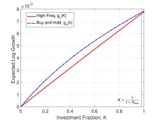
Figure 1: Expected Log-Growth with $n=100$

Fractional Kelly Strategies: The optimum above for $p=0.6$ requires that almost all funds be invested in the underlying stock. Since this might be viewed as far too aggressive for many traders, many authors suggest using a so-called fractional Kelly strategy. This is obtained by scaling down the fraction $K$ so that the investment level is lower; e.g., see [4], [5], [14] and [15]. Now if one uses a fractional Kelly strategy for the binary lattice model above, as seen in Figure V, the “margin of victory” for the buy and holder can be larger. In fact, $g_{n}(K)>g_{1}(K)$ for the entire open interval $0<K<1$.

Binary Lattice with Variable Probability: We now revisit the binary lattice example above with the same parameters $X_{\max}=0.02$, $X_{\min}=-0.01$ and $n=100$, but now let the probability $p$ vary. Recalling the analysis in the previous subsection, when there is no delay, the trade is sufficiently attractive if $p>0.34.$ Thus, within this range of $p$, for the no-delay case, the buy and holder matches the performance of the high-frequency trader. However, when a unit execution delay is in play, Figure V shows that the buy and holder becomes the “winner.” The plot of the percentage difference $(g_{n}^{*}-g_{1}^{*})/g_{1}^{*}\times 100\%$ versus $p$ in this figure shows an increasing “margin of victory” for the buy and holder as $p$ varies over its range.

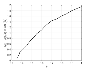
Figure 2: $(g_{n}^{*}-g_{1}^{*})/g_{1}^{*}\times 100\%$ Versus $p$

VI Conclusion and Future Work

In this paper, we studied a stock trading problem using Kelly’s expected logarithmic growth criterion as the performance metric. We first proved a theorem showing that high-frequency trading is unbeatable when there are no transaction costs and no execution delays. Then, when delay in execution is considered, we showed, using a binary lattice model, that there are cases when trading at high-frequency can be inferior to buy and hold. The binary lattice stock model used in Section V is based on a mathematical model with returns $X(k)$ which are larger than those seen with real “high-frequency” trading data. Thus, it is important to ask whether the buy and holder can still achieve a higher ELG than a high-frequency trader based on a real-world model obtained from historical data. This situation is discussed below.

Testing with Historical Data: In this subsection, we provide a gateway to future research by describing how the ideas in this paper might be further pursued using historical intra-day tick data instead of a mathematical price model. For such data, each “tick” corresponds to a new stock price, and the time between order book transactions can be as low as a microsecond. Let $t$ and $s$ denote the arrays of time stamps and transaction prices, respectively. For a trader confronted with an execution delay of $\Delta t$, in seconds the prices used for simulation are selected as follows: If a trade occurs at $t(k)$, the next trading time which one should use occurs at time $t(k^{\prime})$ where

$$k^{\prime}=\min\{i:t(i)\geq t(k)+\Delta t\}.$$

With the convention above, we obtain a subsequence $t(k_{j})$ of $t(k)$ with total number of trades denoted by $m$, and we work with the associated stock prices $s(k_{j})$ and the corresponding returns

$$x_{j}\doteq\frac{s(k_{j+1})-s(k_{j})}{s(k_{j})}.$$

These returns define an empirical probability mass function given by the sum of impulses

$$\widehat{f}_{{}_{X}}(x)=\frac{1}{m}\sum_{j=0}^{m-1}\delta(x-x_{j}),$$

which is used to generate random returns for the Monte-Carlo simulation which is needed to maximize expected logarithmic growth going forward.

Using the procedure above with $\Delta t=1$, we conducted a preliminary experiment using high-frequency historical intra-day tick data for APPLE (ticker AAPL) for the period 9:30:00 AM to 10:00:00 AM on December 2, 2015. We obtained $m=1293$ trades with approximately $1.4$ seconds as the mean value of $t(k_{j+1})-t(k_{j})$. Our Monte-Carlo simulation, carried out using $50,000$ sample paths for each value of $K$, resulted in optimal fractions are $K_{1}^{*}=K_{n}^{*}\approx 0.9978$ and associated optimal ELGs $g_{1}^{*}\approx 3.9966\times 10^{-6}$ and $g_{n}^{*}\approx 4.002\times 10^{-6}$. Since the difference between these quantities is too small to rule out roundoff error, we deemed our simulation to be inconclusive as to which of the two traders achieves better performance. Another confounding factor to mention is that in our simulation, both traders own between $85.1$ and $85.5$ shares during the entirety of the thirty minutes of market time under consideration. In conclusion, studies of ELG performance using real market data are relegated to future research.

Other Future Research Directions: Regarding further research on delay-related issues, another interesting direction would be to extend our results in trade execution to also include delay in information acquisition. A second additional direction of future research is motivated by the fact that we only dealt with a single stock in this paper. In the future, we envision a formulation which involves a portfolio with multiple stocks. Our preliminary work to date suggests that a generalization of the High-Frequency Maximality Theorem given in Section III should be possible to obtain. If this proves to be true, such a result would serve as a good starting point for future work.

References

- [1] J. L. Kelly, “A New Interpretation of Information Rate,” Bell System Technical Journal, vol. 35.4, pp. 917–926, 1956.
- [2] N. H. Hakansson, “On Optimal Myopic Portfolio Policies With and Without Serial Correlation of Yields,” Journal of Business, vol. 44, pp. 324-334, 1971.
- [3] R. C. Merton, Continuous Time Finance, Wiley-Blackwell, 1992.
- [4] E. O. Thorp, “The Kelly Criterion in Blackjack Sports Betting and The Stock Market,” Handbook of Asset and Liability Management: Theory and Methodology, vol. 1, pp. 385–428, Elsevier Science, 2006.
- [5] L. C. MacLean, E. O. Thorp, and W. T. Ziemba “Long-term Capital Growth: The Good and Bad Properties of The Kelly and Fractional Kelly Capital Growth Criteria,” Quantitative Finance, vol. 10, pp. 681–687, 2010.
- [6] T. M. Cover and J. A. Thomas, Elements of Information Theory, John Wiley and Sons, 2006.
- [7] D. G. Luenberger, Investment Science, Oxford University Press, 2013.
- [8] C. H. Hsieh, B. R. Barmish, and J. A. Gubner, “Kelly Betting Can Be Too Conservative,” Proceedings of the IEEE Conference on Decision and Control, pp. 3695-3701, Las Vegas, 2016.
- [9] L. C. MacLean, E. O. Thorp, and W. T. Ziemba, The Kelly Capital Growth Investment Criterion: Theory and Practice, World Scientific Publishing Company, 2011.
- [10] D. Kuhn and D. G. Luenberger, “Analysis of the Rebalancing Frequency in Log-Optimal Portfolio Selection,” Quantitative Finance, vol. 10, pp. 221–234, 2010.
- [11] S. R. Das, D. Kaznachey and M. Goyal, “Computing Optimal Rebalance Frequency for Log-Optimal Portfolios,” Quantitative Finance, vol. 14, pp.1489–1502, 2014.
- [12] C. H. Hsieh, B. R. Barmish, and J. A. Gubner, “At What Frequency Should the Kelly Bettor Bet,” Proceedings of the American Control Conference, pp. 5485–5490, Milwaukee, 2018.
- [13] C. H. Hsieh, J. A. Gubner, and B. R. Barmish, “Rebalancing Frequency Considerations for Kelly-Optimal Stock Portfolios in a Control-Theoretic Framework,” Proceedings of the IEEE Conference on Decision and Control, pp. 5820–5825, Miami, 2018.
- [14] N. Rujeerapaiboon, B. R. Barmish and D. Kuhn, “On Risk Reduction in Kelly Betting Using the Conservative Expected Value,” Proceedings of the IEEE Conference on Decision and Control, pp. 5801–5806, Miami, 2018.
- [15] M. Davis and S. Lleo, “Fractional Kelly Strategies for Benchmarked Asset Management,” in L. C. MacLean, E. O. Thorp, and W. T. Ziemba, The Kelly Capital Growth Investment Criterion: Theory and Practice, World Scientific, pp. 385-407, 2010.
- [16] B. R. Barmish and J. A. Primbs, “On a New Paradigm for Stock Trading Via a Model-Free Feedback Controller,” IEEE Transactions on Automatic Control, AC-61, pp. 662-676, 2016.