The analysis of the excited bottom and bottom strange states $B_{1}(5721)$, $B_{2}^{*}(5747)$, $B_{s1}(5830)$, $B_{s2}^{*}(5840)$, $B_{J}(5840)$ and $B_{J}(5970)$ in B meson family.

Abstract

In order to make a further confirmation about the assignments of the excited bottom and bottom strange mesons $B_{1}(5721)$, $B_{2}^{*}(5747)$, $B_{s1}(5830)$, $B_{s2}^{*}(5840)$ and meanwhile identify the possible assignments of $B_{J}(5840)$, $B_{J}(5970)$, we study the strong decays of these states with the ${}^{3}P_{0}$ decay model. Our analysis support $B_{1}(5721)$ and $B_{2}^{*}(5747)$ to be the $1P_{1}^{\prime}$ and $1^{3}P_{2}$ assignments and the $B_{s1}(5830)$, $B_{s2}^{*}(5840)$ to be the strange partner of $B_{1}(5721)$ and $B_{2}^{*}(5747)$. Besides, we tentatively identify the recently observed $B_{J}(5840)$, $B_{J}(5970)$ as the $2^{3}S_{1}$ and $1^{3}D_{3}$ states, respectively. It is noticed that this conclusion needs further confirmation by measuring the decay channel to $B\pi$ of $B_{J}(5840)$ and $B_{J}(5970)$ in experiments.
Key words: Bottom mesons, ${}^{3}P_{0}$ model, Strong decays
PACS: 13.25.Ft, 14.40.Lb

1 Introduction

In recent decades, theoretical and experimental physicists have made a progress in studying the heavy-light meson spectrum with the observation of a large number of charmed and bottom mesons. Especially, the charmed meson spectrum has been mapped out with high precision with the observation of many new charmed states such as $D_{1}^{*}(2680)$, $D_{2}^{*}(2460)$, $D_{J}(2580)$, $D_{J}^{*}(2650)$, $D_{J}^{*}(2760)$, $D_{J}(2740)$, $D_{J}(3000)$, $D_{J}^{*}(3000)$, etc.Aaij1 ; Aaij2 ; Del1 . In our previous work, we studied the strong decay behaviors of some charmed states with the ${}^{3}P_{0}$ decay model and the heavy meson effective theory, and identified the quantum numbers of these charmed statesGuo1 ; Wang1 ; Wang2 . Whereas for bottom sector, only the ground states, $B^{0}(5279)$, $B^{\pm}(5279)$, $B^{*}(5324)$, $B_{s}(5366)$, $B_{s}^{*}(5415)$ and a few of low lying excited states, $B_{1}(5721)$, $B_{2}^{*}(5747)$ have been identified in PDGPDG . Comparing with the charmed mesons, we know little about the information of most of the excited bottom states

Fortunately for us, the LHCb collaboration have observed some new bottom states in recent years, such as $B_{J}(5721)^{0}$, $B_{J}(5721)^{+}$, $B_{2}^{*}(5747)^{0}$, $B_{2}^{*}(5747)^{+}$, $B_{J}(5840)^{0}$, $B_{J}(5840)^{+}$, $B_{J}(5970)^{0}$, $B_{J}(5970)^{+}$B1 ; B2 ; B3 ; B7 . Besides, CDF, D0 and LHCb collaborations have also observed two bottom strange mesons, $B_{s1}(5830)$, $B_{s2}^{*}(5840)$B4 ; B5 ; B6 and assigned its $J^{P}$ to be $1^{+}$ and $2^{+}$, respectively. The masses and the widths of these newly observed bottom and bottom strange mesons are listed in Table I. For these mesons, an important work is to identify its quantum numbers and assign a place in the bottom meson spectrum. We can adopt several approaches to carry out this work such as quark modelM1 ; M2 ; M3 , Heavy Quark Effective Theory(HQET)M4 ; Wang1 , lattice QCDLattice1 and ${}^{3}P_{0}$ model3P01 ; 3P02 ; 3P03 etc. However, the predictions obtaining from different theoretical approaches, even the same theoretical method with different parameters are not completely consistent with each other.

Table 1: The experimental information about the excited bottom and bottom strange states in this paper.

States	Mass(MeV/c2)	Width(MeV)	$J^{PC}$	Decay channels
$B_{1}(5721)^{+}$ PDG	$5725.9^{+2.5}_{-2.7}MeV$	$31\pm 6MeV$	$1^{+}$	$B^{*0}\pi^{+}$
$B_{1}(5721)^{0}$PDG	$5726.1\pm 1.3MeV$	$27.5\pm 3.4MeV$	$1^{+}$	$B^{*+}\pi^{-}$
$B_{2}^{*}(5747)^{+}$PDG	$5737.2\pm 0.7MeV$	$20\pm 5$	$2^{+}(1^{3}P_{2})$	$B^{0}\pi^{+}$, $B^{*0}\pi^{+}$
$B_{2}^{*}(5747)^{0}$PDG	$5739.5\pm 0.7$	$24.2\pm 1.7$	$2^{+}(1^{3}P_{2})$	$B^{+}\pi^{-}$, $B^{*+}\pi^{-}$
$B_{J}(5970)^{+}$PDG	$5964\pm 5MeV$	$62\pm 20$	-	$B^{*0}\pi^{+}$, [$B^{0}\pi^{+}$]
$B_{J}(5970)^{0}$PDG	$5971\pm 5MeV$PDG	$81\pm 12$	-	$B^{*0}\pi^{+}$, [$B^{+}\pi^{-}$]
$B_{J}(5840)^{+}$B7	$5862.9\pm 5.0$	$224\pm 80MeV$	-	$B^{*0}\pi^{+}$, [$B^{0}\pi^{+}$]
$B_{J}(5840)^{0}$B7	$5862.9\pm 5.0$	$127.4\pm 16.7MeV$	-	$B^{*0}\pi^{+}$, [$B^{+}\pi^{-}$]
$B_{s1}(5830)$PDG	$5828.7\pm 0.1$	$0.5\pm 0.3$	$1^{+}$	$B^{*}K$
$B_{s2}^{*}(5840)$PDG	$5839.85\pm 0.7$	$1.40\pm 0.4$	$2^{+}(1^{3}P_{2})$	$B^{*}K$,$BK$

Since the discoveries of the bottom mesons $B_{1}(5721)$ and $B_{2}^{*}(5747)$ by the $D0$ collaboration in 2007B1 , people studied its nature with different models and identified these two mesons as the $1^{+}$ and $2^{+}$ bottom states in PDGPDG . However, it is still need confirmation for the assignments of the $B_{1}(5721)$ meson because it is the mixing of the ${}^{3}P_{1}$ and ${}^{1}P_{1}$ states. For $B_{J}(5970)$ bottom meson, it was mainly explained to be a $2S1^{-}$ or $1D3^{-}$ state by different theoretical approaches701 ; 702 ; 703 ; 704 ; 705 ; 706 ; 707 . And its spin parity still remain undetermined in the PDG, which only listed its mass and decay width. Further more, we note that the $B_{J}(5840)$ meson was omitted from the summary tables in the PDG, which indicates that the assignment of this meson needs more theoretical and experimental verifications. As for the $B_{s2}^{*}(5840)$ and $B_{s1}(5830)$ bottom-strange mesons, people assigned these two mesons as the strange parters of $B_{2}^{*}(5747)$ and $B_{1}(5721)$ with quantum numbers to be $2^{+}$ and $1^{+}$ respectivelyPDG ; 301 ; 302 ; 303 ; 304 .

In our previous work, we studied the two-body strong decays of the $B_{1}(5721)$, $B_{2}^{*}(5747)$, $B(5970)$, $B_{s1}(5830)$ and $B_{s2}(5840)$ with the heavy meson effective theory in the leading order approximation, and assigned states $2S1^{-}$, $1D1^{-}$ and $1D3^{-}$ as the candidate of $B_{J}(5970)$701 . As a continuation of our previous work, we study the strong decay behaviors of more bottom mesons with the ${}^{3}P_{0}$ decay model and give a simple discussion about the quantum numbers of these mesons. The calculated strong decay widths in this work will be confronted with the experimental data in the future and will be helpful in determining the nature of these heavy-light mesons. This article is arranged as follows: In section 2, we give a brief review of the ${}^{3}P_{0}$ decay model; in Sec.3 we study the strong decays of $B_{1}(5721)$, $B_{2}^{*}(5747)$, $B_{s1}(5830)$, $B_{s2}^{*}(5840)$, $B_{J}(5840)$ and $B_{J}(5970)$ and identify the assignments of these states; in Sec.4, we present our conclusions.

2 Strong decay model

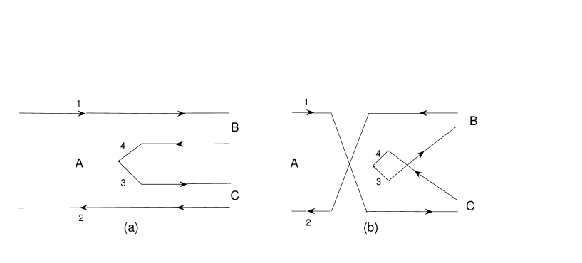
Figure 1: The two possible diagrams contributing to $A\rightarrow BC$ in the ${}^{3}P_{0}$ model.

To study the strong decay properties of the mesons, the ${}^{3}P_{0}$ decay model is an effective and simple method, which can give a good prediction about the decay behaviors of many hadrons3P1 ; 3P2 ; 3P3 ; 3P4 ; 3P5 . This model was first introduced by Micu in 19693P01 and further developed by Le Yaouanc and other collaborations3P02 ; 3P03 . In Ref.Barnes Barnes et al. performed a comprehensive study of light meson strong decays with the ${}^{3}P_{0}$ model. Now, this model has been extensively used to describe the strong decays of the heavy mesons in the charmonium3P6 ; 3P7 ; 3P8 ; 3P9 and bottommonium systems3P10 ; 3P11 ; 3P12 , the baryons3P13 and even the teraquark states3P14 .

At first, people considered an alternative phenomenological model to study the strong decays, in which quark-antiquark pairs are produced with ${}^{3}S_{1}$ quantum numbers. However, this possibility is disfavoured by measuring ratios of partial wave amplitudesGeiger . In ${}^{3}P_{0}$ decay model, it is now generally accepted that a quark-antiquark pair($q_{3}\overline{q}_{4}$) with $0^{++}$ quantum numbers(in the ${}^{3}P_{0}$ state) is created from the vacuum3P01 ; 3P02 ; 3P03 ; 3P1 . For a meson decay process $A$$\rightarrow$$BC$, the quark-antiquark pair($q_{3}\overline{q}_{4}$) regroups into final state mesons($BC$) with the $q_{1}\overline{q}_{2}$ from the initial meson $A$. This process is illustrated in FIG.1 and its transition operator in the nonrelativistic limit is written as,

$$\begin{split}T=&-3\gamma\sum_{m}\langle 1m1-m\mid 00\rangle\int d^{3}\vec{p}_{3}d^{3}\vec{p}_{4}\delta^{3}(\vec{p}_{3}+\vec{p}_{4})\mathcal{Y}_{1}^{m}(\frac{\vec{p}_{3}-\vec{p}_{4}}{2})\chi_{1-m}^{34}\varphi_{0}^{34}\omega_{0}^{34}q_{3}^{{\dagger}}(\vec{p}_{3})q_{4}^{{\dagger}}(\vec{p}_{4})\end{split}$$ (1)

where $q_{3}^{{\dagger}}$ and $q_{4}^{{\dagger}}$ are the creation operators in the momentum-space for the quark-antiquark $q_{3}\overline{q}_{4}$ pair. $\gamma$ is a dimensionless parameter reflecting the creation strength of the quark-antiquark pair. $\varphi_{0}^{34}$, $\omega_{0}^{34}$ and $\chi_{1-m}^{34}$ denote its flavor, color and spin wave functions.

In the c.m. frame, the amplitude of a decay process $A\rightarrow BC$ can be written as,

$$\mathcal{M}^{M_{J_{A}}M_{J_{B}}M_{J_{C}}}(\vec{P})= \gamma\sqrt{8E_{A}E_{B}E_{C}}\sum_{\mbox{\tiny$\begin{array}[]{c}M_{L_{A}},M_{S_{A}},\\ M_{L_{B}},M_{S_{B}},\\ M_{L_{C}},M_{S_{C}},m\end{array}$}}\langle L_{A}M_{L_{A}}S_{A}M_{S_{A}}\mid J_{A}M_{J_{A}}\rangle\langle L_{B}M_{L_{B}}S_{B}M_{S_{B}}\mid J_{B}M_{J_{B}}\rangle$$ (2)

$$\times\langle L_{C}M_{L_{C}}S_{C}M_{S_{C}}\mid J_{C}M_{J_{C}}\rangle\langle 1m1-m\mid 00\rangle\langle\chi_{S_{B}M_{S_{B}}}^{14}\chi_{S_{C}M_{S_{C}}}^{32}\mid\chi_{S_{A}M_{S_{A}}}^{12}\chi_{1-m}^{34}\rangle$$

$$\times\Big{[}\langle\phi_{B}^{14}\phi_{C}^{32}\mid\phi_{A}^{12}\phi_{0}^{34}\rangle I(\vec{P},m_{1},m_{2},m_{3})$$

$$+(-1)^{1+S_{A}+S_{B}+S_{C}}\langle\phi_{B}^{32}\phi_{C}^{14}\mid\phi_{A}^{12}\phi_{0}^{34}\rangle I(-\vec{P},m_{2},m_{1},m_{3})\Big{]},$$

where $\langle\chi_{S_{B}M_{S_{B}}}^{14}\chi_{S_{C}M_{S_{C}}}^{32}\mid\chi_{S_{A}M_{S_{A}}}^{12}\chi_{1-m}^{34}\rangle$, $\langle\phi_{B}^{14}\phi_{C}^{32}\mid\phi_{A}^{12}\phi_{0}^{34}\rangle$ are the spin and flavor matrix elements. The two terms in the last factor correspond to the two possible diagrams in FIG.1. The momentum space integral $I(\vec{P},m_{1},m_{2},m_{3})$ is given by

$$\begin{split}I(\vec{P},m_{1},m_{2},m_{3})=&\int d^{3}\vec{p}\psi^{*}_{n_{B}L_{B}M_{L_{B}}}(\frac{m_{3}}{m_{1}+m_{2}}\vec{P}_{B}+\vec{p})\psi^{*}_{n_{C}L_{C}M_{L_{C}}}(\frac{m_{3}}{m_{2}+m_{3}}\vec{P}_{B}+\vec{p})\\ &\times\psi_{n_{A}L_{A}M_{L_{A}}}(\vec{P}_{B}+\vec{p})\mathcal{Y}_{1}^{m}(\vec{p})\end{split}$$ (3)

where $\vec{P}=\vec{P}_{B}=-\vec{P}_{C},\vec{p}=\vec{p}_{3}$, $m_{3}$ is the mass of the created quark $q_{3}$. In Eq.(3), $\psi$ is the simple harmonic oscillator (SHO) function which is use to describe the space part of the meson. In momentum space, it is defined as

$$\begin{split}\Psi_{nLM_{L}}(\vec{p})=&(-1)^{n}(-i)^{L}R^{L+\frac{3}{2}}\sqrt{\frac{2n!}{\Gamma(n+L+\frac{3}{2})}}exp(-\frac{R^{2}p^{2}}{2})L_{n}^{L+\frac{1}{2}}(R^{2}p^{2})\mathcal{Y}_{LM_{L}}(\vec{p})\end{split}$$ (4)

where $R$ is the scale parameter of the SHO. With the Jacob-Wick formula, we can convert the helicity amplitude into the partial wave amplitude

$$\begin{split}\mathcal{M}^{JL}(\vec{P})=&\frac{\sqrt{4\pi(2L+1)}}{2J_{A}+1}\sum_{M_{J_{B}}M_{J_{C}}}\langle L0JM_{J_{A}}|J_{A}M_{J_{A}}\rangle\langle J_{B}M_{J_{B}}J_{C}M_{J_{C}}|JM_{J_{A}}\rangle\mathcal{M}^{M_{J_{A}}M_{J_{B}}M_{J_{C}}}(\vec{P})\end{split}$$ (5)

where $M_{J_{A}}=M_{J_{B}}+M_{J_{C}}$, $\mathbf{J_{A}=J_{B}+J_{C}}$ and $\mathbf{J_{A}+J_{P}=J_{B}+J_{C}+L}$.

The decay width in terms of partial wave amplitudes using the relative phase space is

$$\Gamma=\frac{\pi}{4}\frac{|\vec{P}|}{M_{A}^{2}}\sum_{JL}|\mathcal{M}^{JL}|^{2}$$ (6)

where $P=|\vec{P}|=\frac{\sqrt{[M_{A}^{2}-(M_{B}+M_{C})^{2}][M_{A}^{2}-(M_{B}-M_{C})^{2}]}}{2M_{A}}$ is the three momentum of the daughter mesons in the c.m. frame. $M_{A}$, $M_{B}$, and $M_{C}$ are the masses of the mesons $A$, $B$, and $C$, respectively. One can consult references3P01 ; 3P02 ; 3P03 ; 3P1 for more details of the decay model.

3 The results and discussions

The parameters involved in the ${}^{3}P_{0}$ model include the light quark pair($q\overline{q}$) creation strength $\gamma$, the SHO wave function scale parameter $R$, and the masses of the mesons and the constituent quarks. First, the masses of the quark are taken as $m_{u}=m_{d}=0.22$ GeV, $m_{s}=0.42$ GeV and $m_{b}=4.81GeV$PDG . Second, as for the factor $\gamma$, it describes the strength of quark-antiquark pair creation from the vacuum and its value needs to be fitted according to experimental data. We take the fitted value $\gamma=6.25$ for $u/d$ quark and $\gamma_{s\overline{s}}=\gamma/\sqrt{3}$ for $s$ quark3P1 . This value is higher than that used by Kokoski and Isgur by a factor of $\sqrt{96\pi}$ due to different field theory conventions, constant factors in $T$, etcKokoski .

The input parameter $R$ has a significant influence on the shape of the radial wave function, which lead to the spatial integral of Eq.(3) being sensitive to the parameter $R$. Thus, the decay width based on the ${}^{3}P_{0}$ decay model is also sensitive to the parameter $R$. Taking the strong decay of $B_{2}^{*}(5747)$ as an example, we plot the decay width versus the input parameters $R$ in FIG.2. We can clearly see the dependence of the decay widths on the input parameter $R$. If the $R_{B^{0}}$, $R_{B^{+}}$, $R_{B^{*0}}$, $R_{B^{*+}}$ and $R_{\pi}$ are fixed to be $2.5GeV^{-1}$, the decay width of $B_{2}^{*}(5747)$ changes several times with the value of $R_{B_{2}^{*}(5747)}$ changing from $2.0GeV^{-1}$ to $3.0GeV^{-1}$. As for this problem, there are two kinds of choices which are the common value and the effective value. The effective value is fixed to reproduce the realistic root mean square radius by solving the Schrodinger equation with a linear potential. For the common value, H.G. Blunder et al3P1 carry out a series of least squares fits of the model predictions to the decay widths of $28$ of the best known meson decays. And the common oscillator parameter $R$ with the vaue $2.5GeV^{-1}$ is suggested to be optimal. In our previous work, we studied strong decays of some charmed mesons with common value and obtained consistent results with experimental data. Thus, we still adopt common value as the input of $R$ in this work.

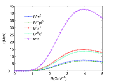
Figure 2: The strong decay of $B^{*+}_{2}(5747)$ as the $1^{3}P_{2}$ state on scale parameter $R$.

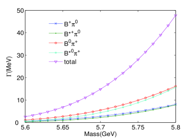
Figure 3: The strong decay of $B^{*+}_{2}(5747)$ as the $1^{3}P_{2}$ state on the mass.

Table 2: The adopted masses of the hadrons used in our calculations.

States	$\pi^{\pm}$	$\pi^{0}$	$\eta$	$B^{\pm}$	$B^{0}$
Mass(MeV)	$139.6$	$135.0$	$547.9$	$5279.3$	5279.6
States	$B^{*}$	$B_{s}^{0}$	$B_{s}^{*}$	$K^{\pm}$	$\overline{K^{0}}$
Mass(MeV)	$5324.7$	$5366.9$	$5415.4$	$493.67$	$497.61$

Finally, the mass of the meson has also a significant influence on the strong decay of the studied meson. For $B_{2}^{*}(5747)$ as an example, if the masses of the daughter mesons are taken to be the standard values in PDG, the decay widths of $B_{2}^{*}(5747)$ vary greatly with its mass, which can be seen in FIG.3. We know that the masses of the bottom mesons, especially the newly observed bottom states, have been updated from time to time. In this work, we take the recently updated values in PDGPDG as the input and list these values in TABLE II. As for the newly observed bottom states which were omitted in PDG, we take the experimental data as the input.

It is noticed that mixing can occur between states with $J=L$ and $S=1$ or $S=0$. The relation between the heavy quark symmetric states and the non-relativistic states ${}^{3}L_{L}$ and ${}^{1}L_{L}$ is written asMatsuki ,

$${\left(\begin{array}[]{ccc}|s_{l}=L+\frac{1}{2},L^{P}\rangle\\ |s_{l}=L-\frac{1}{2},L^{P}\rangle\end{array}\right)}=\frac{1}{\sqrt{2L+1}}{\left(\begin{array}[]{ccc}\sqrt{L+1}&-\sqrt{L}\\ \sqrt{L}&\sqrt{L+1}\end{array}\right)}{\left(\begin{array}[]{ccc}|^{3}L_{L}\\ |^{1}L_{L}\end{array}\right)}$$ (7)

For the states $J=L=1$, the mixture angle is $\theta=-54.7^{\circ}$ or $\theta=35.3^{\circ}$, thus this relation transforms into

$${\left(\begin{array}[]{ccc}|\frac{3}{2},1^{+}\rangle\\ |\frac{1}{2},1^{+}\rangle\end{array}\right)}={\left(\begin{array}[]{ccc}cos\theta&-sin\theta\\ sin\theta&cos\theta\end{array}\right)}{\left(\begin{array}[]{ccc}|^{3}P_{1}\\ |^{1}P_{1}\end{array}\right)}$$ (8)

For a decay process $A\rightarrow BC$, if the initial states $A(l^{P})$are the mixture, the partial wave amplitude can be written as

$${\left(\begin{array}[]{ccc}\mathcal{M}^{JL}_{|l+\frac{1}{2},l^{P}\rangle\rightarrow BC}\\ \mathcal{M}^{JL}_{|l-\frac{1}{2},l^{P}\rangle\rightarrow BC}\end{array}\right)}={\left(\begin{array}[]{ccc}cos\theta&-sin\theta\\ sin\theta&cos\theta\end{array}\right)}{\left(\begin{array}[]{ccc}\mathcal{M}^{JL}_{|^{3}l_{l}\rangle\rightarrow BC}\\ \mathcal{M}^{JL}_{|^{1}l_{l}\rangle\rightarrow BC}\end{array}\right)}$$ (9)

In our calculations, the states $B_{1}(5721)$, $B_{s1}(5830)$ are the $1^{+}$ bottom and bottom-strange states and each of them is the mixing of ${}^{3}P_{1}$ and ${}^{1}P_{1}$ states. In addition, we will study the strong decays of $B_{J}(5970)$ as the $2^{-}$ state and it is the mixture of ${}^{3}D_{2}$ and ${}^{1}D_{2}$ states. Considering the mixture of the initial states, the decay width can be expressed as

$$\Gamma(|l+\frac{1}{2},l^{P}\rangle\rightarrow BC)=\frac{\pi}{4}\frac{|\overrightarrow{P}|}{M_{A}^{2}}\sum_{JL}|cos\theta\mathcal{M}^{JL}_{|^{3}L_{L}\rightarrow BC}-sin\theta\mathcal{M}^{JL}_{|^{1}L_{L}\rightarrow BC}|^{2}$$

$$\Gamma(|l-\frac{1}{2},l^{P}\rangle\rightarrow BC)=\frac{\pi}{4}\frac{|\overrightarrow{P}|}{M_{A}^{2}}\sum_{JL}|sin\theta\mathcal{M}^{JL}_{|^{3}L_{L}\rightarrow BC}+cos\theta\mathcal{M}^{JL}_{|^{1}L_{L}\rightarrow BC}|^{2}$$

3.1 $B_{2}^{*}(5747)$, $B_{1}(5721)$, $B^{*}_{0}$

Table 3: The strong decay widths of the $B_{2}^{*}(5747)$, $B_{1}(5721)$, $B^{*}_{0}$ with possible assignments. If the corresponding decay channel is forbidden, we mak it by ”-”. All values in units of $MeV$.

	$B_{2}^{*+}(5747)$	$B_{1}^{+^{\prime}}(5721)$	$B_{1}^{+}(5721)$	$B^{*+}_{0}$
State	$1^{3}P_{2}$	$1P_{1}^{\prime}$	$1P_{1}$	$1^{3}P_{0}$
Mass	$5737.2$PDG	$5726.0$PDG	$5726.0$PDG	$5697.4$707
$B^{+}\pi^{0}$	$4.3$	$-$	$-$	$76.3$
$B^{*+}\pi^{0}$	$3.7$	$26.5$	$138.8$	$-$
$B^{0}\pi^{+}$	$8.6$	$-$	$-$	$155.1$
$B^{*0}\pi^{+}$	$7.3$	$13.3$	$69.4$	$-$
total	$23.9$	$39.8$	$208.2$	$231.4$

Table 4: The strong decay widths of the $B_{2}^{*}(5747)$, $B_{1}(5721)$, $B^{*}_{0}$ with possible assignments. If the corresponding decay channel is forbidden, we mak it by ”-”. All values in units of $MeV$.

	$B_{2}^{*0}(5747)$	$B_{1}^{0^{\prime}}(5721)$	$B_{1}^{0}(5721)$	$B^{*0}_{0}$
State	$1^{3}P_{2}$	$1P_{1}^{\prime}$	$1P_{1}$	$1^{3}P_{0}$
Mass	$5739.5$PDG	$5726.1$PDG	$5726.1$PDG	$5697.4$707
$B^{+}\pi^{-}$	$8.9$	$-$	$-$	$78.3$
$B^{*+}\pi^{-}$	$7.6$	$25.3$	$134.9$	$-$
$B^{0}\pi^{0}$	$4.4$	$-$	$-$	$156.5$
$B^{*0}\pi^{0}$	$3.8$	$12.6$	$67.6$	$-$
total	$24.7$	$37.9$	$202.5$	$234.8$

The bottom mesons $B_{2}^{*+}(5747)$, $B_{2}^{*0}(5747)$ are assigned to be the $2^{+}$ state with their total decay widths to be $20\pm 5MeV$ and $24.2\pm 1.7MeV$, respectively. As the $1^{3}P_{2}(2^{+})$ states, we calculate their strong decay widths and the results $23.9MeV$ and $24.7MeV$ for $B_{2}^{*+}(5747)$, $B_{2}^{*0}(5747)$ are consistent well with these experimental data. A further confirmation of this assignment is the predicted versus measured ratio of partial widths to $B^{0}\pi^{+}$ and $B^{*0}\pi^{+}$. The predicted partial ratio

$$\frac{\Gamma_{B_{2}^{*+}(5747)\rightarrow B^{0}\pi^{+}}}{\Gamma_{B_{2}^{*+}(5747)\rightarrow B^{*0}\pi^{+}}}=1.18$$

is in agreement with the experimental data $1.12$, and so does for the $B_{2}^{*0}(5747)$. As for $B_{1}^{+}(5721)$, $B_{1}^{0}(5721)$ mesons, each of them is the mixing bottom state of ${}^{3}P_{1}$ and ${}^{1}P_{1}$. In TABLE III and TABLE IV, the $1P_{1}$, $1P_{1}^{{}^{\prime}}$ states denote the $j_{q}=\frac{1}{2}$ and $j_{q}=\frac{3}{2}$ state, respectively. We can see that the results for $j_{q}=\frac{3}{2}(1P_{1}^{{}^{\prime}})$ bottom states with total decay widths to be $39.8MeV$, $37.9MeV$, are roughly compatible with the experimental data $31\pm 6MeV$ and $27.5\pm 3.4MeV$. These results favor $B_{1}(5721)$ to be the $j_{q}=\frac{3}{2}$ spin partner of $B_{2}^{*}(5747)$ state

$$(B_{1}(5721),B_{2}^{*}(5747))=(1^{+},2^{+})_{\frac{3}{2}}\qquad n=1,L=1$$

After identifying the $1P_{1}^{\prime}$ assignment, the remaining $1P_{1}$ together with $1^{3}P_{0}$ state are the spin doublets with $j_{q}=\frac{1}{2}$. The total widths of $1^{3}P_{0}$ are predicted to be $231.4MeV$, which is broader comparing with those of $j_{q}=\frac{3}{2}$ P-wave doublets. This prediction is consistent with that of the heavy quark limit(HQL).

3.2 $B_{J}(5840)$, $B_{J}(5970)$

Table 5: The strong decay widths of the $B_{J}^{+}(5840)$, $B_{J}^{+}(5970)$ with possible assignments. If the corresponding decay channel is forbidden, we mak it by ”-”. All values in units of $MeV$

	$B_{J}^{+}(5840)$		$B_{J}^{+}(5970)$
States	$2^{1}S_{0}$	$2^{3}S_{1}$	$2^{3}S_{1}$	$1^{3}D_{1}$	$1^{3}D_{3}$	$1D_{2}^{\prime}$	$1D_{2}$
Mass	$5862.9$B7		$5964$PDG
$B^{+}\pi^{0}$	$-$	$12.9$	$10.2$	$27.3$	$6.5$	$-$	$-$
$B^{*+}\pi^{0}$	$38.1$	$25.4$	$23.7$	$14.1$	$6.0$	$23$	$80.9$
$B^{0}\pi^{+}$	$-$	$25.8$	$20.4$	$54.6$	$13.1$	$-$	$-$
$B^{0*}\pi^{+}$	$76.1$	$50.8$	$47.4$	$28.2$	$11.9$	$11.6$	$40.5$
$B^{+}\eta$	$-$	$2.7$	$14.4$	$25.8$	$0.5$	$-$	$-$
$B^{*+}\eta$	$-$	$1.6$	$20.0$	$8.5$	$0.5$	$1.2$	$23.4$
$B_{S}^{0}K^{+}$	$-$	$-$	$13.1$	$21.4$	$0.2$	$-$	$-$
$B_{S}^{0*}K^{+}$	$-$	$-$	$12.3$	$4.9$	$0.03$	$0.6$	$13.9$
total	$114.2$	$121.9$	$171.5$	$194.3$	$38.7$	$36.4$	$158.7$

Table 6: The strong decay widths of the $B_{J}^{0}(5840)$, $B_{J}^{0}(5970)$ with possible assignments. If the corresponding decay channel is forbidden, we mak it by ”-”. All values in units of $MeV$.

	$B_{J}^{0}(5840)$B7		$B_{J}^{0}(5970)$
States	$2^{1}S_{0}$	$2^{3}S_{1}$	$2^{3}S_{1}$	$1^{3}D_{1}$	$1^{3}D_{3}$	$1D_{2}^{\prime}$	$1D_{2}$
Mass	$5862.9$B7		$5971.0$PDG
$B^{+}\pi^{-}$	$-$	$25.8$	$20.0$	$54.3$	$13.4$	$-$	$-$
$B^{*+}\pi^{-}$	$76.1$	$50.8$	$46.7$	$28.3$	$12.2$	$22.9$	$80.9$
$B^{0}\pi^{0}$	$-$	$12.9$	$10.0$	$27.1$	$6.7$	$-$	$-$
$B^{0*}\pi^{0}$	$38.0$	$25.3$	$23.3$	$14.1$	$6.1$	$11.4$	$40.5$
$B^{0}\eta$	$-$	$2.7$	$14.7$	$26.3$	$0.5$	$-$	$-$
$B^{*0}\eta$	$-$	$-$	$20.9$	$8.9$	$0.2$	$1.3$	$23.9$
$B_{S}^{0}K^{+}$	$-$	$-$	$13.7$	$22.1$	$0.2$	$-$	$-$
$B_{S}^{0*}K^{+}$	$-$	$-$	$13.5$	$5.2$	$0.03$	$0.6$	$13.5$
total	$114.1$	$117.5$	$162.8$	$186.3$	$39.3$	$36.2$	$158.8$

We notice that the PDG only reported the $B_{J}(5970)$ bottom meson and omitted the $B_{J}(5840)$ state from the summary tables, and the spin-parity of $B_{J}(5970)$ was unknown. Thus, we study the strong decay behaviors with the $2^{1}S_{0}$, $2^{3}S_{1}$ assignments for $B_{J}(5840)$ state and $2^{3}S_{1}$, $1^{3}D_{1}$, $1^{3}D_{3}$, $1D_{2}^{\prime}$, $1D_{2}$ assignments for $B_{J}(5970)$ state. The results are showed in TABLE V and TABLE VI. The LHCb collaboration has suggested that the $B_{J}(5840)$, $B_{J}(5970)$ signals should be identified with the $2^{1}S_{0}$ and $2^{3}S_{1}$ bottom states. We note also that the $B\pi$ decay mode is reported by LHCb as ’possibly seen’ for the strong decays of $B_{J}(5840)$ and $B_{J}(5970)$. However, our analysis indicate that the decay mode to $B\pi$ is forbidden for $B_{J}(5840)$ as a $2^{1}S_{0}$ assignment. If the decay to $B\pi$ is confirmed in the future, the $2^{1}S_{0}$ assignment can be ruled out. As the $2^{3}S_{1}$ assignments for $B_{J}^{+}(5840)$ and $B_{J}^{0}(5840)$, their total decay widths are $121.9MeV$ and $117.5MeV$, and these values are compatible with the experimental data. Overall, we tentatively identify $2^{3}S_{1}$ as the assignment of $B_{J}(5840)$.

The same with $B_{J}(5840)$, the decay channel $B\pi$ of $B_{J}(5970)$ is ’possibly seen’ in experiments, so the assignments $1D_{2}^{{}^{\prime}}$ and $1D_{2}$ are tentatively ruled out as the decay to $B\pi$ is forbidden. The experiments suggested the total decay widths for $B_{J}^{+}(5970)$ and $B_{J}^{0}(5970)$ are $62\pm 20MeV$ and $81\pm 12MeV$. For the assignments $1^{3}D_{3}$ and $1^{3}D_{1}$, we can see that the predicted total widths of $1^{3}D_{3}$ assignments, $38.7MeV$ and $39.3MeV$, are consistent with the experiments within the predictive power of the model and experimental uncertainties. Thus, we slightly prefer the $1^{3}D_{3}$ assignment of the $B_{J}(5970)$. Certainly, the conclusion about the assignments depend strongly on the accurate measurement of the decay mode $B\pi$ of $B_{J}(5840)$ and $B_{J}(5970)$.

3.3 $B_{s1}(5830)$, $B_{s2}^{*}(5840)$, $B_{s0}^{*}$

Table 7: The strong decay widths of the $B_{s2}^{*}(5840)$, $B_{s0}^{*}$, $B_{s1}(5830)$ with possible assignments. If the corresponding decay channel is forbidden, we mak it by ”-”. All values in units of $MeV$.

	$B_{s2}^{*}(5840)$	$B_{s0}^{*}$	$B_{s1}(5830)$
States	$1^{3}P_{2}$	$1^{3}P_{0}$	$1P_{1}^{\prime}$	$1P_{1}$
Mass	$5839.85$PDG	$5794.8$707	$5828.7$PDG	$5828.7$PDG
$B^{+}K^{-}$	$0.6$	$217$	$-$	$-$
$B^{*+}K^{-}$	$0.09$	$-$	$1.59$	$31.9$
$B_{0}\overline{K^{0}}$	$0.6$	$217$	$-$	$-$
$B_{0}^{*}\overline{K^{0}}$	$0.06$	$-$	$1.51$	$30.2$
total	$1.35$	$434$	$3.1$	$62.1$

The bottom strange mesons $B_{s1}(5830)$ and $B_{s2}^{*}(5840)$ are identified as the $1^{+}$ and $2^{+}$ assignments in PDG, but it is noted that the $J^{P}$ need confirmationPDG . In order to give a further confirmation, we study the strong decay behaviors of $B_{s2}^{*}(5840)$ as the $1^{3}P_{2}$ assignment and $B_{s1}(5830)$ as the $1P_{1}^{\prime}$, $1P_{1}$ assignments. The predicted total decay width of $B_{s2}^{*}(5840)$ is $1.35MeV$ and it is consistent well with the experimental data $1.40\pm 0.4$. In addition, the predicted partial decay ratio

$$\frac{\Gamma_{B_{s2}^{*}(5840)\rightarrow B^{*+}K^{-}}}{\Gamma_{B_{s2}^{*}(5840)\rightarrow B^{+}K^{-}}}=0.15$$ (10)

This value is roughly compatible with the experimental data $0.093\pm 0.018$, which supports $1^{3}P_{2}$ to be the assignment of $B_{s2}^{*}(5840)$. As a $1^{+}$ state, $B_{s1}(5830)$ meson is the mixture between $1^{3}P_{1}$ and $1^{1}P_{1}$. From the results in TABLE VII, we can see that the predicted total decay width of $1P_{1}^{\prime}$ is $3.1MeV$ and this value is consistent with the experimental data $0.5\pm 0.4MeV$ within the predictive power of the model. Thus, the $1P_{1}^{\prime}$ is the optimal assignment for $B_{s1}(5830)$ and we can conclude that $B_{s1}(5830)$ and $B_{s2}^{*}(5840)$ are the $j_{q}=\frac{3}{2}$ doublets,

$$(B_{s1}(5830),B_{s2}^{*}(5840))=(1^{+},2^{+})_{\frac{3}{2}}\qquad n=1,L=1$$

Again, the remaining states $1P_{1}$ and $1^{3}P_{0}$ in TABLE VII are the spin doublets with $j_{q}=\frac{1}{2}$ and their total decay widths are much broader than those of the spin doublets with $j_{q}=\frac{3}{2}$.

4 Conclusion

In summary, we study the two-body strong decays of the excited bottom and bottom strange states $B_{1}(5721)^{0}$, $B_{1}(5721)^{+}$, $B_{2}^{*}(5747)^{0}$, $B_{2}^{*}(5747)^{+}$, $B_{J}(5840)^{0}$, $B_{J}(5840)^{+}$, $B_{J}(5970)^{0}$, $B_{J}(5970)^{+}$, $B_{s1}(5830)$, $B_{s2}^{*}(5840)$ with the ${}^{3}P_{0}$ decay model. By analyzing the decay properties of these mesons, we further confirm the assignments of $B_{1}(5721)$, $B_{2}^{*}(5747)$, $B_{s1}(5830)$, $B_{s2}^{*}(5840)$ and identify the possible assignments of $B_{J}(5840)$, $B_{J}(5970)$. Our analysis support $B_{1}(5721)$ and $B_{2}^{*}(5747)$ are the spin doublets $(1^{+},2^{+})_{\frac{3}{2}}$ with $n=1$, $L=1$ and $B_{s1}(5830)$, $B_{s2}^{*}(5840)$ are the strange partner of $B_{1}(5721)$ and $B_{2}^{*}(5747)$. The possible assignments for $B_{J}(5840)$, $B_{J}(5970)$ are $2^{3}S_{1}$ and $1^{3}D_{3}$, which need further confirmation in experiments. Especially, the decay of $B_{J}(5840)$, $B_{J}(5970)$ state to $B\pi$ is crucial to identifying the optimal assignments for these states.

Acknowledgment

This work has been supported by the Fundamental Research Funds for the Central Universities, Grant Number $2016MS133$ and Natural Science Foundation of HeBei Province, Grant Number A2018502124.

References

(1) R. Aaij et al [LHCb Collaboration], Phys. Rev. D 94,072001(2016).
(2) R. Aaij et al [LHCb Collaboration], JHEP 145, 1309(2013).
(3) P. del Amo Sanchez et al [BaBar Collaboration], Phys. Rev. D 82, 111101(2010).
(7) M. Tanabashi et al. (Particle Data Group), Phys. Rev. D 98, 030001(2018).
(8) V. M. Abazov et al, Phys. Rev. Lett. 99,172001(2007).
(9) T. Aaltonen et al, Phys. Rev. Lett. 102,102003(2009).
(10) T. Aaltonen et al, Phys. Rev. D 90, 012013(2014)[arXiv:1309.5961].
(11) R. Aaij et al. [LHCb Collaboration],JHEP 024,1504(2015).
(12) T. Aaltonen et al, Phys. Rev. Lett. 100,082001(2008).
(13) V. Abazov et al, Phys. Rev. Lett. 100,082002(2008).
(14) R. Aaij et al, Phys. Rev. Lett. 110,151803(2013).
(15) S. Godfrey and N. Isgur,Phys. Rev. D 32,189 (1985).
(16) D. Ebert, R. N. Faustov and V. O. Galkin, Eur. Phys. J. C66,197(2010).
(17) L. Y. Xiao and X. H. Zhong, Phys. Rev. D 90, 074029(2014).
(18) P. Colangelo et. al., Phys. Rev. D 86, 054024 (2012).
(19) C. B. Lang, Daniel Mohler, Sasa Prelovsek, et al, Phys. Lett. B750,17(2015).
(20)L. Micu, Nucl. Phys. B 10, 521 (1969).
(21) R. Carlitz and M. Kislinger, Phys. Rev. D 2, 336 (1970); E. W.
Colglazier and J. L. Rosner, Nucl. Phys. B 27, 349 (1971); W. P.
Petersen and J. L. Rosner, Phys. Rev. D 6, 820 (1972).
(22)A. Le Yaouanc, L. Oliver, O. Pene, and J.-C. Raynal, Phys. Rev. D 8,
2223 (1973); 9, 1415 (1974); 11, 1272 (1975); Phys. Lett. B 71, 397
(1977); A. Le Yaouanc, L. Oliver, O. Pene, and J. C. Raynal, Phys.
Lett. B 72,57(1977).
(32)Zhi-Feng Sun, Ju-Jun Xie, E. Oset, arXiv:1801.04367.
(33)Xiu-Lei Ren, Zhi-Feng Sun, Phys. Rev. D 99, 094041(2019).
(34)H. G. Blundell, arXiv:hep-ph/9608473; H. G. Blundell and
S. Godfrey, Phys. Rev. D 53, 3700 (1996); H. G. Blundell, S.
Godfrey, and B. Phelps, Phys. Rev. D 53, 3712 (1996).
(35)H. Q. Zhou, R. G. Ping, and B. S. Zou, Phys. Lett. B 611,
123 (2005).
(36)D.-M. Li and S. Zhou, Phys. Rev. D 78, 054013 (2008); D.-M. Li and
E. Wang, Eur. Phys. J. C 63, 297 (2009); D.-M. Li, P.-F. Ji, and B.
Ma, Eur. Phys. J. C 71, 1582 (2011).
(37)B. Zhang, X. Liu, W. Z. Deng, and S. L. Zhu, Eur. Phys. J. C 50,
617 (2007); Y. Sun, Q. T. Song, D. Y. Chen, X. Liu, and S. L. Zhu,
Phys. Rev. D 89, 054026 (2014).
(39)T. Barnes, F. E. Close, P. R. Page, and E. S. Swanson, Phys. Rev. D 55, 4157 (1997).
(40)E. S. Ackleh, T. Barnes, and E. S. Swanson, Phys. Rev. D
54, 6811 (1996); T. Barnes, N. Black, and P. R. Page, Phys. Rev. D
68, 054014 (2003); T. Barnes, S. Godfrey, and E. S. Swanson, Phys.
Rev. D 72, 054026 (2005).
(41)J. Ferretti, G. Galata, and E. Santopinto, Phys. Rev. C 88,
015207 (2013).
(42)P. G. Ortega, J. Segovia, D. R. Entem and F. Fernandez, arXiv:1706.02639.
(43)J. Ferretti, G. Galata, and E. Santopinto, Phys. Rev.
D 90, 054010 (2014).
(44)J. Ferretti and E. Santopinto, Phys. Rev. D 90,
094022 (2014).
(45)F. E. Close and E. S. Swanson, Phys. Rev. D 72, 094004
(2005); F. E. Close, C. E. Thomas, O. Lakhina, and E. S. Swanson,
Phys. Lett. B 647, 159 (2007).
(46)J. Segovia, D.R. Entem, F. Fernandez, Phys. Lett. B
715, 322 (2012).
(47)Ze Zhao, Dan-Dan Ye, and Ailin Zhang,Phys. Rev. D 95, 114024
(2017).
(48)Xue-wen Liu, Hong-Wei Ke, Xiang Liu, Xue-Qian Li, Eur. Phys. J. C 76, 549 (2016).
(49)P. Geiger and E. Swanson, Phys. Rev. D50, 6855 (1994).
(50)R. Kokoski and N. Isgur, Phys. Rev. D35,907(1987).
(51)T. Matsuki, T. Morii, K. SEO, Prog. Theor. Phys. 124,285(2010).