Latency Minimization for Multiuser Computation Offloading in Fog-Radio Access Networks

Abstract

This paper considers computation offloading in fog-radio access networks (F-RAN), where multiple user equipments (UEs) offload their computation tasks to the F-RAN through a number of fog nodes. Each UE can choose one of the fog nodes to offload its task, and each fog node may serve multiple UEs. Depending on the computation burden at the fog nodes, the tasks may be computed by the fog nodes or further offloaded to the cloud via capacity-limited fronthaul links. To compute all UEs’ tasks as fast as possible, joint optimization of UE-Fog association, radio and computation resources of F-RAN is proposed to minimize the maximum latency of all UEs. This min-max problem is formulated as a mixed integer nonlinear program (MINP). We first show that the MINP can be reformulated as a continuous optimization problem, and then employ the majorization minimization (MM) approach to find a solution. The MM approach that we develop is unconventional in that—each MM subproblem can be solved inexactly with the same provable convergence guarantee as the conventional exact MM, thereby reducing the complexity of each MM iteration. In addition, we also consider a cooperative offloading model, where the fog nodes compress-and-forward their received signals to the cloud. Under this model, a similar min-max latency optimization problem is formulated and tackled again by the inexact MM approach. Simulation results show that the proposed algorithms outperform some heuristic offloading strategies, and that the cooperative offloading can better exploit the transmission diversity to attain better latency performance than the non-cooperative one.

Index terms—Fog-radio access networks, Fog computing, Majorization minimization, WMMSE.

I Introduction

The next generation wireless communication system is expected to provide ubiquitous connections for massive heterogenous Internet of Things (IoT) devices with high speed and low latency. The current cloud-computing-based network infrastructure is facing challenges to meet these requirements, because massive heterogenous requests with different data size and latency requirements need to be forwarded to and processed at the central baseband processing units (BBUs), which, however, could cause heavy burden on the fronthaul, and incur intolerable latency for some delay-critical missions. For example, in some interactive applications, e.g., virtual reality, industrial automation and vehicle-to-vehicle communications, the round-trip delay may be required below a few tens of milliseconds [1]. To meet the critical latency requirement and alleviate the pressure on the fronthaul, a fog-computing-based radio access network (F-RAN) has recently been proposed as a promising solution [2]. The concept of F-RAN is developed from the fog computing, which was originally proposed by Cisco [3]. By shifting certain amount of computing, storage and networking functions from the cloud to the edge of the network, F-RAN is able to provide more prompt responses to users’ requests with less fronthaul bandwidth occupation.

Evolving from cloud RAN (C-RAN) to F-RAN, the wireless access point (AP) is endowed with more capabilities and functions, such as computation and content caching. In this work, we focus on the computation aspect of F-RAN, and investigate how the enhanced APs (also called fog nodes in the rest of the paper) near the user equipments (UEs) can help improve the latency performance in the fog-assisted computation offloading applications. Conventionally, computation offloading has been extensively studied in the context of mobile-edge computation (MEC) [4, 5, 6, 7]. MEC considers that there is one or multiple computing servers to process the tasks, which are partially or wholly offloaded by UEs. The offloading is usually accomplished via wireless transmissions from UEs to the MEC server, and the UEs are competing with each other for the radio and computation resources. To provide satisfactory quality-of-service (QoS) for UEs, a joint optimization of the offloading decision and resource allocation is the crux of achieving efficient MEC.

Earlier studies on MEC focused on the offloading decision-making for single UE admission. By assuming infinite computation capacity of the server, the trade-off between the offloading and local computation was thoroughly investigated in [8, 9, 10]. Recently, more efforts have been devoted to joint optimization of offloading decision, communication and computation resource allocations. Typically, this kind of problems are formulated as mixed-integer nonlinear programs (MINP) with different utility functions. In [11, 12, 13] the authors studied the MEC problem with the goal of minimizing the total energy consumption, including transmission and computation energy, subject to UEs’ latency requirements. CCCP [11], quantized dynamic programming [12] and Lagrangian duality method [13] are employed to find approximate solutions for the MINP. In [14, 15, 16, 17, 18, 19], the latency is adopted as the system utility function. The work [14] developed an iRAR algorithm to minimize the sum latency for multiple base stations (BSs) and multiple computing servers. For the case of single computing server, the work [15] derived the optimal resource allocations under local computing, cloud computing and mixed computing models. Different from [14, 15], the work [16, 19] studied the worst-case latency minimization problem in order to provide latency fairness for UEs. By extending the fireworks algorithm to the binary case, a heuristic offloading decision and resource allocation scheme was proposed. To balance energy consumption and latency, the weighted energy-plus-latency utility function is also commonly adopted in MEC offloading [20, 21, 22, 23, 24]. Apart from the above models, there are also other MEC models, which are proposed to address some specific issues in offloading, such as dynamic environment change, online and distributed implementations of offloading schemes; see [25, 26, 27, 28, 29, 30, 31] and the references therein.

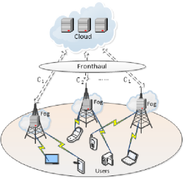
Figure 1: F-RAN model.

Back to F-RAN, this work focuses on the fog-assisted computation offloading. Different from the above MEC models, the fog-assisted computation offloading model consists of three layers, the UE layer, the fog layer and the cloud layer; see Figure 1 for an illustration. Each UE offloads its computation task to F-RAN via one of the fog nodes. The tasks may be processed by the fog nodes or further offloaded to the cloud, depending on the computation and the fronthaul capacities of the fog nodes. To guarantee fairness, a min-max latency minimization criterion is adopted herein to optimize the F-RAN resources—which include the UE-Fog association, radio and computation resources—so that the worst latency of all UEs induced by transmission and computation is as small as possible. This min-max latency optimization problem is formulated as an MINP. With a careful treatment of the binary variables, we show that the MINP can be equivalently reformulated into a form involving only continuous variables, and thereby powerful machinery in continuous optimization can be exploited to handle it. Specifically, by incorporating the idea of majorization minimization (MM) [32] and the weighted MMSE (WMMSE) reformulation [33], we develop an inexact MM algorithm for the min-max problem with convergence guarantee to a Karush-Kuhn-Tucker (KKT) solution.

We should mention that the aforementioned min-max fairness problem assumes that each fog node individually forwards the associated UE’s task to the cloud, if the task is processed at the cloud. To fully capture the cooperative gain of the fog nodes, we also consider a cooperative offloading strategy, where all the fog nodes compress-and-forward their received signals to the cloud. With cooperative offloading, the UE-to-cloud channel can be seen as a virtual multiple-access channel (V-MAC). By applying a similar discrete-to-continuous variable reformulation, an inexact MM algorithm is developed to find a solution. Simulation results demonstrate that the cooperative offloading can generally provide better latency performance as compared with the non-cooperative one.

I-A Related Works and Contributions

There are some related works worth mentioning. The works [34] and [35, 36] considered a joint optimization of radio and computation resources for energy minimization with latency constraints in single-cell and multicell networks, respectively, where all the computation is done at the cloud with the UE-BS association prefixed. In [37, 38], a cooperative computation model is considered, but their focus is more on choosing appropriate number of fog nodes for each task, given the communication resource constraints. The latency minimization, the energy minimization and the energy-plus-delay minimization are respectively considered in [21, 22, 39], [40] and [16, 41] under the setting of multiple UEs, one computing AP (or fog node) and a cloud server. The work [42] studied the optimal computation task scheduling problem in order to minimize the total latency. Since there is only one computing AP, no UE-AP association optimization is needed and moreover transmit beamforming is not considered in [21, 22, 39, 40, 16, 41, 42]. The work [23] deals with a similar problem as [21, 22, 43] under the multi-fog setting, however, beamforming and cooperative offloading among fog nodes is again not considered. The work [44] studied a hybrid communication and computation offloading problem in F-RAN by jointly optimizing the UE-AP association and the bandwith allocation. A genetic convex optimization algorithm (GCOA) was proposed to divide the original MINP into two convex optimization problems. Apart from the optimization-based approach, learning-based offloading decision approach has also attracted much attention recently. In particular, the works [45, 46, 47, 48, 49] proposed deep reinforcement learning and federated learning methods to centralized or decentralized learn the offloading policy. Besides computation offloading decision, there are other works investigating F-RAN from various perspectives, including the offloading performance analysis [50, 51, 52], energy efficiency optimization [53, 54] and cache deployment [55, 56], to name a few; see [57] and the references therein.

To summarize, compared with the existing works on F-RAN, the main contributions of this work are as follows.

1. We consider a general compuation offloading model in F-RAN, which include transmit beamforming between multiple multi-antenna UEs and multiple multi-antenna fog nodes, UE-fog association, fog-cloud computation task distribution and cooperative computation offloading among fog nodes. To the best of our knowledge, this comprehensive model has not been touched in the current literature.

2. Aiming at providing latency fairness for all UEs, we formulate a min-max delay problem by jointly optimizing the UE-fog association, the fog-cloud task distribution, radio and computation resource allocation. This min-max problem is a MINLP problem in its original form. We show that it can be equivalently transformed into a pure continuous optimization problem. Upon the latter, an inexact MM-based block-coordinate descent (BCD) method is proposed, and its convergence to a KKT point is also proved.

3. We have conducted extensive numerical simulations to demonstrate the efficacy of the proposed offloading scheme. Especially, simulation results reveal that under some conditions, the proposed cooperative offloading via compression-and-forward among fog nodes attains superior performance over the non-cooperative one. To the best of our knowledge, this is the first work that investigates advantage of cooperative offloading via compression-and-forward in the F-RAN.

I-B Organization and Notations

This paper is organized as follows. The system model and problem statement are given in Section II. Section III develops an inexact MM approach to tackling the min-max latency optimization problem. Section IV considers a cooperative fog-assisted offloading model and develops an iterative algorithm to optimize the resources. Simulation results comparing the proposed designs are illustrated in Section V. Section VI concludes the paper.

Our notations are as follows. $(\cdot)^{T}$ and $(\cdot)^{H}$ denote the transpose and conjugate transpose, respectively; $\bm{I}$ denotes an identity matrix with an appropriate dimension; $\mathbb{C}^{N}$ denotes the set of complex vectors of dimension $N$; $\bm{A}\succeq\mathbf{0}$ (respectively $\bm{A}\succ\mathbf{0}$) means that $\bm{A}$ is Hermitian positive semidefinite (respectively definite); ${\rm Tr}(\cdot)$ denotes a trace operation; ${\rm Diag}({\bm{A}},{\bm{B}})$ represents a block diagonal matrix with the diagonal blocks $\bm{A}$ and $\bm{B}$; $\mathcal{CN}(\bm{a},\bm{\Sigma})$ represents a complex Gaussian distribution with mean $\bm{a}$ and covariance matrix $\bm{\Sigma}$.

II System Model and Problem Statement

Consider an F-RAN, consisting of $K$ multi-antenna UEs, $L$ fog nodes and a cloud server. Each UE has a computation task, however, due to limited computation capacity, all the tasks have to be offloaded to the F-RAN via the fog nodes. Suppose the user $k$’s task ${\sf T}_{k}$ is described by a two-tuple of $(D_{k},B_{k})$ integers, where $D_{k}$ denotes the number of flops needed for completing ${\sf T}_{k}$, and $B_{k}$ represents the number of bits needed for encoding ${\sf T}_{k}$. To offload the task to F-RAN, user $k$ has to send the $B_{k}$ bits to the fog nodes through wireless transmission. For simplicity, we assume that each user gets access to F-RAN through one of the fog nodes, while each fog node may simultaneously provide access for multiple users. The association between the fog nodes and the users is not prefixed and needs to be jointly optimized with other resources. To highlight this, we introduce a binary variable $\alpha_{k,\ell}\in\{0,~{}1\}$ to indicate the association. In particular,

$$\alpha_{k,\ell}=\begin{cases}1,&\mbox{if user $k$ is connected with fog $\ell$},\\ 0,&\mbox{otherwise,}\end{cases}$$

and $\sum_{\ell=1}^{L}\alpha_{k,\ell}=1,~{}\forall~{}k\in{\cal K}\triangleq\{1,\ldots,K\}$.

Now, the offloading process can be described in the following two stages:

Stage 1: Wireless Transmissions from Users to Fog Nodes. For ease of exposition, let us assume that user $k$ is associated with fog node $\ell\in{\cal L}\triangleq\{1,\ldots,L\}$, i.e., $\alpha_{k,\ell}=1$ and $\alpha_{k,\ell^{\prime}}=0,\forall\ell^{\prime}\neq\ell$. Let

$$\bm{x}_{k}(t)=\bm{v}_{k}s_{k}(t)\in\mathbb{C}^{N_{k}},\quad k\in\cal K$$

be the transmit signal of UE $k$, where $\bm{v}_{k}\in\mathbb{C}^{N_{k}}$ is the transmit beamformer with $N_{k}$ being the number of transmit antennas, and $s_{k}(t)\in\mathbb{C}$ is the encoded signal for task ${\sf T}_{k}$. Then, the received signal at the fog $\ell$ is given by

$$\bm{y}_{\ell}(t)=\bm{H}_{k,\ell}^{H}\bm{v}_{k}s_{k}(t)+\textstyle\sum_{j\neq k}\bm{H}_{j,\ell}^{H}\bm{v}_{j}s_{j}(t)+\bm{n}_{\ell}(t),$$

where $\bm{H}_{j,\ell}\in\mathbb{C}^{N_{j}\times M_{\ell}}$ is the channel between UE $j$ and fog $\ell$ with $M_{\ell}$ being the number of antennas at fog $\ell$, and $\bm{n}_{\ell}(t)\sim{\cal CN}(\bm{0},\sigma_{\ell}^{2}\bm{I})$ is additive white Gaussian noise. The communication rate between UE $k$ and fog $\ell$ is given by

$$R_{k,\ell}=W\log(1+\bm{v}_{k}^{H}\bm{H}_{k,\ell}(\sigma_{\ell}^{2}\bm{I}+\sum_{j\neq k}\bm{H}_{j,\ell}^{H}\bm{v}_{j}\bm{v}_{j}^{H}\bm{H}_{j,\ell})^{-1}\bm{H}_{k,\ell}^{H}\bm{v}_{k})$$ (1)

where $W$ (Hz) is the bandwidth of the wireless transmission. The corresponding wireless transmission latency is

$$\tau_{k,\ell}^{T}=\frac{B_{k}}{R_{k,\ell}}.$$ (2)

Stage 2: Computing at the Fog Nodes/Cloud. After the reception, the fog node $\ell$ may compute the task by itself or further offload the task to the cloud, depending on the fog’s computation load and the complexity of ${\sf T}_{k}$. There are two cases:

1. Computing ${\sf T}_{k}$ at the fog node. Let $f_{k,\ell}^{F}$ be the number of CPU flops allocated for executing ${\sf T}_{k}$ in every second. Then, the computation latency is

   $$\tau_{k,\ell}^{F}=\frac{D_{k}}{f_{k,\ell}^{F}}.$$ (3)

2. Computing ${\sf T}_{k}$ at the cloud. In such a case, the processing latency consists of two parts. One is transmission latency from the fog node to the cloud, and the other is the computation latency at the cloud. We consider that fog $\ell$ is connected with the cloud via fronthaul with limited capacity $C_{\ell,\max}$ (bits/second). Let $C_{k,\ell}(\leq C_{\ell,\max})$ be the fronthaul capacity allocated by fog $\ell$ for further offloading ${\sf T}_{k}$ to the cloud. Then, the processing latency at the cloud is given by

   $$\tau_{k,\ell}^{C}=\frac{B_{k}}{C_{k,\ell}}+\frac{D_{k}}{f_{k}^{C}},$$ (4)

   where $f_{k}^{C}$ is the number of CPU flops allocated by the cloud to execute ${\sf T}_{k}$ in every second.

To differentiate the above two cases, we introduce a binary variable $\beta_{k}\in\{0,~{}1\}$ to indicate where the computation is performed. In particular,

$$\beta_{k}=\begin{cases}0,&\mbox{if the fog performs computation,}\\ 1,&\mbox{if the cloud performs computation.}\end{cases}$$

Based on the above offloading model, our goal is to optimize the communication and computation resources, so that the maximum latency among UEs is minimized:

$$\min_{\begin{subarray}{c}\{\bm{v}_{k},f_{k}^{C},\beta_{k}\}_{k},\\ \{f_{k,\ell}^{F},C_{k,\ell},\alpha_{k,\ell}\}_{k,\ell}\end{subarray}}\max_{k\in{\cal K}}~{}\sum_{\ell=1}^{L}\alpha_{k,\ell}\left(\tau_{k,\ell}^{T}+(1-\beta_{k})\tau_{k,\ell}^{F}+\beta_{k}\tau_{k,\ell}^{C}\right)$$

$$\hskip 28.45274pt{\rm s.t.}\quad f_{k,\ell}^{F}\leq\alpha_{k,\ell}(1-\beta_{k})F_{\ell,\max},~{}\forall~{}k,\ell,$$ (5a)

$$\hskip 42.67912pt~{}\sum_{k=1}^{K}f_{k,\ell}^{F}\leq F_{\ell,\max},\quad f_{k,\ell}^{F}\geq 0,~{}\forall~{}k,\ell,$$ (5b)

$$\hskip 42.67912pt~{}f_{k}^{C}\leq\beta_{k}F_{C,\max},~{}\forall~{}k,$$ (5c)

$$\hskip 42.67912pt~{}\sum_{k=1}^{K}f_{k}^{C}\leq F_{C,\max},\quad f_{k}^{C}\geq 0,~{}\forall~{}k,$$ (5d)

$$\hskip 42.67912pt~{}C_{k,\ell}\leq\alpha_{k,\ell}\beta_{k}C_{\ell,\max},~{}\forall k,~{}\ell,$$ (5e)

$$\hskip 42.67912pt~{}\sum_{k=1}^{K}C_{k,\ell}\leq C_{\ell,\max},~{}C_{k,\ell}\geq 0,~{}\forall~{}k,~{}\ell,$$ (5f)

$$\hskip 42.67912pt~{}\|\bm{v}_{k}\|^{2}\leq P_{k},~{}\forall~{}k,$$ (5g)

$$\hskip 42.67912pt~{}\alpha_{k,\ell}\in\{0,~{}1\},\quad\sum_{\ell=1}^{L}\alpha_{k,\ell}=1,~{}\forall~{}k,$$ (5h)

$$\hskip 42.67912pt~{}\beta_{k}\in\{0,~{}1\},~{}\forall~{}k,$$ (5i)

where $F_{\ell,\max}$ and $F_{C,\max}$ are the maximum number of flops that the fog $\ell$ and the cloud can execute in every second, respectively. The constraints (5a)-(5b) correspond to the computation resource allocation at fog $\ell$. In particular, (5a) implies that fog $\ell$ will allocate computing resource for user $k$ only if $\alpha_{k,\ell}=1$ and $\beta_{k}=0$, i.e., user $k$ is associated with fog $\ell$ and meanwhile the task ${\sf T}_{k}$ is processed at fog $\ell$. Similarly, the constraints (5c)-(5d) correspond to the computation resource allocation at the cloud. The constraints (5e)-(5f) are introduced to account for the finite capacity of fronthaul, and (5g) limits the peak transmit power at the UEs.

Problem (5) is a MINP, which is generally NP-hard. In the next section, we will develop a tractable approach to (5) with a careful treatment of the discrete variables.

III An Inexact MM Approach to Problem (5)

Let us first show that problem (5) can be reformulated as a discrete-variable-free form, and thus continuous optimization approach can be leveraged to handle it. Specifically, we have the following result.

Theorem 1.

The MINP problem (5) is equivalent to the following continuous optimization problem:

$$\min_{\begin{subarray}{c}\{\bm{v}_{k},f_{k}^{C}\},\\ \{f_{k,\ell}^{F},C_{k,\ell},\theta_{k,\ell}^{F},\theta_{k,\ell}^{C}\}\end{subarray}} \max_{k\in{\cal K}}\sum_{\ell=1}^{L}(\theta_{k,\ell}^{F}(\tau_{k,\ell}^{T}+\tau_{k,\ell}^{F})+\theta_{k,\ell}^{C}(\tau_{k,\ell}^{T}+\tau_{k,\ell}^{C}))$$ (6a)

$${\rm s.t.} ~{}~{}\theta_{k,\ell}^{F}\geq 0,\quad\theta_{k,\ell}^{C}\geq 0,~{}\forall~{}k,\ell,$$ (6b)

$$~{}~{}\sum_{\ell=1}^{L}\theta_{k,\ell}^{F}+\theta_{k,\ell}^{C}=1,~{}\forall~{}k,$$ (6c)

$$~{}~{}\eqref{eq:main_c},\eqref{eq:main_e},\eqref{eq:main_g}~{}{\rm and}~{}\eqref{eq:main_a}~{}{\rm satisfied}.$$ (6d)

Proof. See Appendix A. $\blacksquare$

Building upon the above equivalence, we consider solving problem (6). Let us denote $\bm{\theta}_{k}=[\theta_{k,1}^{F},\ldots,\theta_{k,L}^{F},\theta_{k,1}^{C},\ldots,\theta_{k,L}^{C}]^{T}\in\mathbb{R}^{2L}$ and $\bm{\tau}_{k}=[\tau_{k,1}^{T}+\tau_{k,1}^{F},\ldots,\tau_{k,L}^{T}+\tau_{k,L}^{F},\tau_{k,1}^{T}+\tau_{k,1}^{C},\ldots,\tau_{k,L}^{T}+\tau_{k,L}^{C}]^{T}\in\mathbb{R}^{2L}.$ Problem (6) is rewritten as

$$\min_{\begin{subarray}{c}\{\bm{v}_{k},f_{k}^{C},\bm{\tau}_{k},\bm{\theta}_{k}\}_{k},\\ \{R_{k,\ell},f_{k,\ell}^{F},C_{k,\ell}\}_{k,\ell}\end{subarray}}~{}\max_{k\in{\cal K}}~{}\bm{\theta}_{k}^{T}\bm{\tau}_{k}$$ (7a)

$$\hskip 14.22636pt{\rm s.t.}~{}~{}~{}~{}~{}R_{k,\ell}\leq\phi_{k,\ell}(\bm{V}),~{}\forall~{}k,\ell,$$ (7b)

$$\hskip 2.84544pt~{}\tau_{k,\ell}^{T}\geq\frac{B_{k}}{R_{k,\ell}},~{}\tau_{k,\ell}^{F}\geq\frac{D_{k}}{f_{k,\ell}^{F}},~{}\tau_{k,\ell}^{C}\geq\frac{B_{k}}{C_{k,\ell}}+\frac{D_{k}}{f_{k}^{C}},\forall~{}k,\ell,$$ (7c)

$$\hskip 14.22636pt~{}\eqref{eq:main_c},~{}\eqref{eq:main_e},~{}\eqref{eq:main_g},~{}\eqref{eq:main_a},~{}\eqref{eq:main_reform_c},~{}\eqref{eq:main_reform_d}~{}{\rm satisfied}.$$ (7d)

where $\bm{V}\triangleq\{\bm{v}_{k}\}_{k}$ and $\phi_{k,\ell}(\bm{V})\triangleq W\log\Big{(}1+\bm{v}_{k}^{H}\bm{H}_{k,\ell}\big{(}\sigma_{\ell}^{2}\bm{I}+\sum_{j\neq k}\bm{H}_{j,\ell}^{H}\bm{v}_{j}\bm{v}_{j}^{H}\bm{H}_{j,\ell}\big{)}^{-1}\bm{H}_{k,\ell}^{H}\bm{v}_{k}\Big{)}$. Notice that in (7b) and (7c) we have changed the equalities in (1)-(4) as inequalities. This does not incur any loss of optimality because the inequalities in (7b) and (7c) must be active at the optimal solution; for otherwise, we can further decrease $\tau_{k,\ell}^{X},X\in\{T,F,C\}$ and increase $R_{k,\ell}$ to get a lower objective value.

The constraints (7c) and (7d) are convex, but the objective (7a) and the constraint (7b) are still nonconvex. For (7a), we handle it by MM. Let ${\cal X}\triangleq\{\bm{v}_{k},f_{k}^{C},\bm{\tau}_{k},\bm{\theta}_{k}R_{k,\ell},f_{k,\ell}^{F},C_{k,\ell}\}$ be a collection of optimization variables, and ${\cal F}$ be the feasible set of problem (7). The idea of MM is to find a surrogate function $g({\cal X}|\bar{\cal X})$, parameterized by some given point $\bar{\cal X}\in{\cal F}$, for the nonconvex objective (7a) such that the following holds:

$$g({\cal X}|\bar{\cal X}) \geq\max_{k\in{\cal K}}~{}\bm{\theta}_{k}^{T}\bm{\tau}_{k},\forall~{}{\cal X}\in{\cal F},$$ (8)

$$g(\bar{\cal X}|\bar{\cal X}) =\max_{k\in{\cal K}}~{}\bar{\bm{\theta}_{k}}^{T}\bar{\bm{\tau}}_{k}.$$

To this end, we make use of the following fact.

Fact 1.

The function

$$g({\cal X}|\bar{\cal X})=\max_{k\in\cal K}\left\{\frac{\|\bm{\theta}_{k}+\bm{\tau}_{k}\|^{2}}{2}-(\bar{\bm{\theta}}_{k})^{T}\bm{\theta}_{k}-(\bar{\bm{\tau}}_{k})^{T}\bm{\tau}_{k}-\bar{c}_{k}\right\}$$

with $\bar{c}_{k}=\frac{\|\bar{\bm{\theta}}_{k}\|^{2}+\|\bar{\bm{\tau}}_{k}\|^{2}}{2}$ is a surrogate function of $\max_{k\in{\cal K}}~{}\bm{\theta}_{k}^{T}\bm{\tau}_{k}$.

Fact 1 can be easily shown by noting

$$\bm{\theta}_{k}^{T}\bm{\tau}_{k} =\frac{\|\bm{\theta}_{k}+\bm{\tau}_{k}\|^{2}}{2}-\frac{\|\bm{\theta}_{k}\|^{2}+\|\bm{\tau}_{k}\|^{2}}{2}$$

$$\leq\frac{1}{2}\|\bm{\theta}_{k}+\bm{\tau}_{k}\|^{2}-(\bar{\bm{\theta}}_{k})^{T}\bm{\theta}_{k}-(\bar{\bm{\tau}}_{k})^{T}\bm{\tau}_{k}-\bar{c}_{k}$$

for all feasible $(\bar{\bm{\theta}}_{k},\bar{\bm{\tau}}_{k})$, where the inequality is due to the first-order condition for the concave function $-\frac{\|\bm{\theta}_{k}\|^{2}+\|\bm{\tau}_{k}\|^{2}}{2}$. By invoking Fact 1, the MM for problem (7) entails repeatedly performing the following updates:

$${\cal X}^{(t+1)}=\arg\min_{\cal X} ~{}g({\cal X}|{\cal X}^{(t)})$$ (9)

$${\rm s.t.} ~{}\eqref{eq:main_reform2_a}-\eqref{eq:main_reform2_c}~{}{\rm satisfied},$$

for $t=0,1,2,\ldots$ until some stopping criteria is satisfied.

According to the classical convergence result for MM [32], it is well known that every limit point of the iterates generated by (9) is a stationary point of problem (7). However, this convergence result holds under the premise that each MM subproblem is optimally solved. As for the considered problem (9), it may be hard to do so due to the nonconvex constraint (7b). To circumvent this difficulty, we apply the WMMSE method [33] to find an approximate solution for (9). Specifically, define by $\bm{u}_{k,\ell}\in\mathbb{C}^{M}$ the receive beamformer employed by fog $\ell$ to receive user $k$’s signal. Then, the rate function $\phi_{k,\ell}(\bm{V})$ can be alternatively expressed as [33]:

$$\phi_{k,\ell}(\bm{V})=\max_{\bm{u}_{k,\ell},w_{k,\ell}\geq 0}f_{k,\ell}(\bm{u}_{k,\ell},w_{k,\ell},\bm{V})$$ (10)

where

$$f_{k,\ell}(\bm{u}_{k,\ell},w_{k,\ell},\bm{V})\triangleq W\left(-w_{k,\ell}e_{k,\ell}(\bm{u}_{k,\ell},\bm{V})+\log w_{k,\ell}+1\right)$$ (11)

and

$$e_{k,\ell}(\bm{u}_{k,\ell},\bm{V})$$

$$\triangleq \|1-\bm{u}_{k,\ell}^{H}\bm{H}_{k,\ell}^{H}\bm{v}_{k}\|^{2}+\textstyle\sum_{j\neq k}\|\bm{v}_{j}^{H}\bm{H}_{j,\ell}\bm{u}_{k,\ell}\|^{2}+\sigma_{\ell}^{2}\|\bm{u}_{k,\ell}\|^{2}$$

is the MSE of estimating user $k$’s signal at fog $\ell$, when the beamformer $\bm{u}_{k,\ell}$ is used for reception. By substituting (10) into (9), the MM subproblem is equivalently written as

$$\min_{{\cal X},\{\bm{u}_{k,\ell},w_{k,\ell}\}_{k,\ell}} ~{}~{}g({\cal X}|{\cal X}^{(t)})$$ (12)

$${\rm s.t.} ~{}~{}R_{k,\ell}\leq f_{k,\ell}(\bm{u}_{k,\ell},w_{k,\ell},\bm{V}),~{}\forall~{}k,\ell,$$

$$~{}~{}\eqref{eq:main_reform2_b}-\eqref{eq:main_reform2_c}~{}{\rm satisfied}.$$

Problem (12) can be efficiently handled by block-coordinate descent (BCD) method. In particular, given $\bm{V}$ the optimal $\bm{u}_{k,\ell}$ and $w_{k,\ell}$ for (12) is given by [33]

$$\bm{u}_{k,\ell} =(\sigma_{\ell}^{2}\bm{I}+\textstyle\sum_{j=1}^{K}\bm{H}_{j,\ell}^{H}{\bm{v}}_{j}{\bm{v}}_{j}^{H}\bm{H}_{j,\ell})^{-1}\bm{H}_{k,\ell}^{H}\bm{v}_{k},$$ (13a)

$$w_{k,\ell} =e_{k,\ell}^{-1}(\bm{u}_{k,\ell},\bm{V}).$$ (13b)

On the other hand, given $(\bm{u}_{k,\ell},w_{k,\ell})$, problem (12) is convex with respect to the remaining variables, and thus can be optimally solved, say by off-the-shelf software CVX [58]. Theoretically speaking, the above BCD procedure needs to be performed sufficiently large number of rounds in order to obtain a good approximate solution for problem (9). However, this could incur high computational complexity for each MM update. To trade off the solution quality and the computational complexity, we propose a computationally-cheap inexact MM algorithm for problem (7); see Algorithm 1, where for the $t$th MM iteration, we perform only a small number $J^{(t)}$ rounds of BCD update to compute an approximate solution for problem (9). The parameter $J^{(t)}$ controls the solution quality for each MM iteration. While Algorithm 1 performs MM inexactly, the following theorem reveals that the same convergence result as the exact MM (i.e., using the optimal solution of (9) to update ${\cal X}^{(t+1)}$) holds.

Theorem 2.

The iterates $\{{\cal X}^{(t)}\}_{t=0,1,\ldots}$ generated by Algorithm 1 yield a sequence of non-increasing objective values for problem (7). Moreover, every limit point of $\{{\cal X}^{(t)}\}_{t=0,1,\ldots}$ is a KKT point of problem (7).

Proof. See Appendix B. $\blacksquare$

The idea of proving Theorem 2 is that the inexact MM (even for the case of $J^{(t)}=1,\forall~{}t$) is sufficient to provide certain improvement for the objective (7a). By accumulating these improvements, the iterations will finally reside at a KKT point of problem (7).

Algorithm 1 An Inexact MM Approach to (7)

1:Initialize with a feasible point ${\cal X}^{(0)}$, a set of small positive integers $\{J^{(t)}\}_{t=0,1,\ldots}$ and set $t=0$

2:repeat

3:     Set ${\cal X}^{(t_{0})}={\cal X}^{(t)}$;

4:     for $j=0,1,\ldots,J^{(t)}-1$ do

5:         Update $(\bm{u}_{k,\ell}^{(t_{j})},w_{k,\ell}^{(t_{j})})$ according to (13a) and (13b);

6:         Update ${\cal X}^{(t_{j+1})}$ by solving (12) with fixed $(\bm{u}_{k,\ell},w_{k,\ell})=(\bm{u}_{k,\ell}^{(t_{j})},w_{k,\ell}^{(t_{j})})$;

7:     end for

8:     Set ${\cal X}^{(t+1)}={\cal X}^{(t_{j+1})}$;

9:     $t\leftarrow t+1$

10:until some stopping criterion is satisfied

11:Output ${\cal X}^{(t)}$.

IV The Cooperative Offloading Case

In the last two sections, we have considered a two-stage offloading, where each UE’s task is decoded and forwarded to the cloud via the associated fog node, if the task is processed at the cloud. However, this decode-and-forward strategy may not be able to fully exploit the cooperative gain among the fog nodes. In this section, we investigate another forwarding strategy, namely, compress-and-forward, where the fog nodes quantize their received signals using single-user compression, and then transmit the compressed bits to the cloud. By doing so, the UEs’ signals can be simultaneously delivered to the cloud via all the fog nodes. To put it into context, recall the received signal model at the fog nodes

$$\bm{y}_{\ell}(t)=\sum_{k\in{\cal K}}\bm{H}_{k,\ell}^{H}\bm{v}_{k}s_{k}(t)+\bm{n}_{\ell}(t),~{}\forall~{}\ell.$$ (14)

After the reception, the fog $\ell$ quantizes its received signal $\bm{y}_{\ell}$. Assuming Gaussian quantization, the quantized signal $\hat{\bm{y}}_{\ell}(t)$ is given by

$$\hat{\bm{y}}_{\ell}(t)=\bm{y}_{\ell}(t)+\bm{q}_{\ell}(t),~{}\ell\in{\cal L},$$ (15)

where $\bm{q}_{\ell}(t)$ is the quantization noise and follows $\bm{q}_{\ell}(t)\sim{\cal CN}(\bm{0},\bm{Q}_{\ell})$ with $\bm{Q}_{\ell}\succeq\bm{0}$ [59]. Notice that $\bm{Q}_{\ell}$ needs to be jointly optimized with the other resource variables to achieve minimum latency. The quantized signals $\{\hat{\bm{y}}_{\ell}\}_{\ell\in\cal L}$ are then compressed and forwarded to the cloud via the capacity-limited fronthaul links. At the cloud, a two-stage successive decoding strategy is employed—the cloud first recovers the quantized signals $\{\hat{\bm{y}}_{\ell}\}_{\ell\in\cal L}$, and then decodes UEs’ messages $\{s_{k}\}_{k\in\cal K}$ based on the quantized signals $\{\hat{\bm{y}}_{\ell}\}_{\ell\in\cal L}$. Overall, when the compress-and-forward scheme is employed at the fog nodes, the UE-to-cloud channel can be seen as a V-MAC. Following the results in [59] and assuming linear MMSE reception at the cloud, the achievable rate $R_{k,C}$ of UE $k$ for the V-MAC is given by

$$R_{k,C}=W\log(1+\bm{v}_{k}^{H}\bm{H}_{k,{\cal L}}\bm{J}_{k}^{-1}\bm{H}_{k,{\cal L}}^{H}\bm{v}_{k})$$ (16)

where

$$\bm{H}_{k,{\cal L}} =[\bm{H}_{k,1},\ldots,\bm{H}_{k,L}],$$

$$\bm{J}_{k} =\textstyle\sum_{j\neq k}\bm{H}_{j,{\cal L}}^{H}\bm{v}_{j}\bm{v}_{j}^{H}\bm{H}_{j,{\cal L}}+\bm{\Sigma}_{\cal L}+\bm{Q}_{\cal L},$$

$$\bm{\Sigma}_{\cal L} ={\rm Diag}(\sigma_{1}^{2}\bm{I},\ldots,\sigma_{L}^{2}\bm{I}),\quad\bm{Q}_{\cal L}={\rm Diag}(\bm{Q}_{1},\ldots,\bm{Q}_{L}).$$

Since the fog nodes are connected with the cloud via limited-capacity fronthaul, the compression rates at the fog nodes should also satisfy the fronthaul capacity constraints, so that the cloud can correctly recover the quantized signals $\{\hat{\bm{y}}_{\ell}\}_{\ell\in\cal L}$. Specifically, the fronthaul constraint under single-user compression is given by

$$\log\frac{|\sum_{k=1}^{K}\bm{H}_{k,\ell}^{H}\bm{v}_{k}\bm{v}_{k}^{H}\bm{H}_{k,\ell}+\sigma_{\ell}^{2}\bm{I}+\bm{Q}_{\ell}|}{|\bm{Q}_{\ell}|}\leq C_{\ell,\max},~{}\forall~{}\ell\in\cal L.$$

If UE $k$’s task is computed at the cloud, the total latency is calculated as

$$\tau_{k,C}=\frac{B_{k}}{R_{k,C}}+\frac{D_{k}}{f_{k}^{C}}.$$

Now, our min-max latency optimization problem under cooperative offloading is formulated as

$$\min_{\begin{subarray}{c}\{\bm{v}_{k},f_{k}^{C},\beta_{k}\}_{k},\\ \{f_{k,\ell}^{F},\bm{Q}_{\ell},\alpha_{k,\ell}\}_{k,\ell}\end{subarray}}\max_{k\in{\cal K}}~{}\sum_{\ell=1}^{L}\alpha_{k,\ell}\left((1-\beta_{k})(\tau_{k,\ell}^{T}+\tau_{k,\ell}^{F})+\beta_{k}\tau_{k,C}\right)$$

$$\hskip 28.45274pt{\rm s.t.}\quad f_{k,\ell}^{F}\leq\alpha_{k,\ell}(1-\beta_{k})F_{\ell,\max},~{}\forall~{}k,\ell,$$ (17a)

$$\hskip 42.67912pt~{}\sum_{k=1}^{K}f_{k,\ell}^{F}\leq F_{\ell,\max},~{}~{}f_{k,\ell}^{F}\geq 0,~{}\forall~{}k,\ell,$$ (17b)

$$\hskip 42.67912pt~{}f_{k}^{C}\leq\beta_{k}F_{C,\max},~{}\forall~{}k,$$ (17c)

$$\hskip 42.67912pt~{}\sum_{k=1}^{K}f_{k}^{C}\leq F_{C,\max},\quad f_{k}^{C}\geq 0,~{}\forall~{}k,$$ (17d)

$$~{}\log\frac{\left|\displaystyle\sum_{k=1}^{K}\bm{H}_{k,\ell}^{H}\bm{v}_{k}\bm{v}_{k}^{H}\bm{H}_{k,\ell}+\sigma_{\ell}^{2}\bm{I}+\bm{Q}_{\ell}\right|}{|\bm{Q}_{\ell}|}\leq C_{\ell,\max},~{}\forall~{}\ell,$$ (17e)

$$\hskip 42.67912pt~{}\bm{Q}_{\ell}\succeq\bm{0},\quad\forall~{}\ell\in{\cal L},$$ (17f)

$$\hskip 42.67912pt~{}\|\bm{v}_{k}\|^{2}\leq P_{k},~{}\forall~{}k,$$ (17g)

$$\hskip 42.67912pt~{}\alpha_{k,\ell}\in\{0,~{}1\},\quad\textstyle\sum_{\ell=1}^{L}\alpha_{k,\ell}=1,~{}\forall~{}k,$$ (17h)

$$\hskip 42.67912pt~{}\beta_{k}\in\{0,~{}1\},~{}\forall~{}k.$$ (17i)

Similar to problem (5), problem (17) is an MINP. Following the proof of Theorem 1, one can show that problem (17) can be reformulated as the following discrete-variable-free form:

$$\min_{\begin{subarray}{c}\{\bm{v}_{k},f_{k}^{C}\}_{k},\\ \{f_{k,\ell}^{F},\bm{Q}_{\ell},\theta_{k,\ell}^{F},\theta_{k,C}\}\end{subarray}}\max_{k\in{\cal K}}~{}\left\{\theta_{k,C}\tau_{k,C}+\sum_{\ell=1}^{L}\theta_{k,\ell}^{F}(\tau_{k,\ell}^{T}+\tau_{k,\ell}^{F})\right\}$$

$$\hskip 28.45274pt{\rm s.t.}\quad\theta_{k,\ell}^{F}\geq 0,~{}\forall~{}k,\ell,\quad\theta_{k,C}\geq 0,~{}\forall~{}k,$$ (18a)

$$\hskip 42.67912pt~{}\theta_{k,C}+\textstyle\sum_{\ell=1}^{L}\theta_{k,\ell}=1,$$ (18b)

$$\hskip 42.67912pt~{}\eqref{eq:soft_main_c},\eqref{eq:soft_main_e}-\eqref{eq:soft_main_a}~{}{\rm satisfied}.$$ (18c)

Denote $\bm{\theta}_{k}=[\theta_{k,C},~{}\theta_{k,1},\ldots,\theta_{k,L}]\in\mathbb{R}^{L+1}$ and $\bm{\tau}_{k}=[\tau_{k,C},~{}\tau_{k,1}^{T}+\tau_{k,1}^{F},\ldots,\tau_{k,L}^{T}+\tau_{k,L}^{F}]\in\mathbb{R}^{L+1}$. Problem (18) can be reexpressed as

$$\min_{\begin{subarray}{c}\{\bm{v}_{k},f_{k}^{C},\bm{\theta}_{k},\bm{\tau}_{k}\}_{k},\\ \{f_{k,\ell}^{F},\bm{Q}_{\ell}\}\end{subarray}}\max_{k\in{\cal K}}~{}\bm{\theta}_{k}^{T}\bm{\tau}_{k}$$

$${\rm s.t.}~{}R_{k,\ell}\leq W\log\Big{(}1+\bm{v}_{k}^{H}\bm{H}_{k,\ell}\times$$

$$\hskip 36.98866pt(\sigma_{\ell}^{2}\bm{I}+\sum_{j\neq k}\bm{H}_{j,\ell}^{H}\bm{v}_{j}\bm{v}_{j}^{H}\bm{H}_{j,\ell})^{-1}\bm{H}_{k,\ell}^{H}\bm{v}_{k}\Big{)}$$ (19a)

$$\hskip 14.22636pt~{}R_{k,C}\leq W\log(1+\bm{v}_{k}^{H}\bm{H}_{k,{\cal L}}\bm{J}_{k}^{-1}\bm{H}_{k,{\cal L}}^{H}\bm{v}_{k})$$ (19b)

$$\tau_{k,\ell}^{T}\geq\frac{B_{k}}{R_{k,\ell}},\,\tau_{k,\ell}^{F}\geq\frac{D_{k}}{f_{k,\ell}^{F}},\,\tau_{k,C}\geq\frac{B_{k}}{R_{k,C}}+\frac{D_{k}}{f_{k}^{C}},\forall~{}k,\ell,$$ (19c)

$$\log\frac{\left|\displaystyle\sum_{k=1}^{K}\bm{H}_{k,\ell}^{H}\bm{v}_{k}\bm{v}_{k}^{H}\bm{H}_{k,\ell}+\sigma_{\ell}^{2}\bm{I}+\bm{Q}_{\ell}\right|}{|\bm{Q}_{\ell}|}\leq C_{\ell,\max},\forall~{}\ell$$ (19d)

$$\hskip 14.22636pt~{}\eqref{eq:soft_main_a_eqv}-\eqref{eq:soft_main_b_eqv},\eqref{eq:soft_main_c},\eqref{eq:soft_main_e},\eqref{eq:soft_main_g},\eqref{eq:soft_main_a}~{}{\rm satisfied}.$$ (19e)

The constraints (19a)-(19b) can be handled similarly as before by using WMMSE reformulation. Specifically, the constraints (19a) and (19b) can be expressed as

$$R_{k,\ell}\leq f_{k,\ell}(\bm{u}_{k,\ell},w_{k,\ell},\bm{V})$$ (20)

and

$$R_{k,C}\leq f_{k,C}(\bm{u}_{k,C},w_{k,C},\bm{V},\bm{Q}_{\cal L}),$$ (21)

respectively, where $f_{k,\ell}$ is defined in (11), $f_{k,C}(\bm{u}_{k,C},w_{k,C},\bm{V},\bm{Q}_{\cal L})\triangleq W\left(-w_{k,C}e_{k,C}(\bm{u}_{k,C},\bm{V},\bm{Q}_{\cal L})+\log(w_{k,C})+1\right)$, and $e_{k,C}(\bm{u}_{k,C},\bm{V},\bm{Q}_{\cal L})\triangleq\|1-\bm{u}_{k,C}^{H}\bm{H}_{k,{\cal L}}\bm{v}_{k}\|^{2}+\textstyle\sum_{j\neq k}\|\bm{u}_{k,C}^{H}\bm{H}_{j,{\cal L}}\bm{v}_{j}\|^{2}+\bm{u}_{k,C}^{H}(\bm{\Sigma}_{\cal L}+\bm{Q}_{\cal L})\bm{u}_{k,C}$.

As for the fronthaul-capacity constraint (19d), the following lemma is leveraged to recast it into a more tractable form:

Lemma 1 ([60] ).

Let ${\bf E}\in\mathbb{C}^{N\times N}$ be any matrix such that ${\bf E}\succ{\bf 0}$. Consider the function $f({\bf S})=-{\rm Tr}({\bf S}{\bf E})+\ln|{\bf S}|+N$. Then,

$$\ln|{\bf E}^{-1}|=\max_{{\bf S}\in\mathbb{C}^{N\times N},{\bf S}\succeq{\bf 0}}f({\bf S}),$$ (22)

and the optimal ${\bf S}^{\star}={\bf E}^{-1}$.

Applying Lemma 1 to the constraint (19d) yields

$$\max_{\bm{S}_{\ell}\succeq\bm{0}}\{-{\rm Tr}(\bm{S}_{\ell}\bm{E}_{\ell})+\log|\bm{S}_{\ell}|+M_{\ell}\}+\log|\bm{Q}_{\ell}|+C_{\ell,\max}\geq 0,~{}\forall~{}\ell$$ (23)

where $\bm{E}_{\ell}=\sum_{k=1}^{K}\bm{H}_{k,\ell}^{H}\bm{v}_{k}\bm{v}_{k}^{H}\bm{H}_{k,\ell}+\sigma_{\ell}^{2}\bm{I}+\bm{Q}_{\ell}$. By substituting (20), (21) and (23) into (19a), (19b) and (19d), respectively, we can equivalently express problem (19) as

$$\min_{\begin{subarray}{c}\{\bm{v}_{k},\bm{u}_{k},\bm{w}_{k},f_{k}^{C},\bm{\theta}_{k},\bm{\tau}_{k}\}_{k,\ell},\\ \{f_{k,\ell}^{F},\bm{Q}_{\ell},\bm{S}_{\ell},R_{k,\ell}\}_{k,\ell}\end{subarray}}\max_{k\in{\cal K}}~{}\bm{\theta}_{k}^{T}\bm{\tau}_{k}$$ (24)

$${\rm s.t.}~{}~{}R_{k,\ell}\leq f_{k,\ell}(\bm{u}_{k,\ell},w_{k,\ell},\bm{V}),$$

$$\hskip 14.22636pt~{}R_{k,C}\leq f_{k,C}(\bm{u}_{k,C},w_{k,C},\bm{V},\bm{Q}_{\cal L}),$$

$$\hskip 14.22636pt~{}\tau_{k,\ell}^{T}\geq\frac{B_{k}}{R_{k,\ell}},~{}~{}\tau_{k,\ell}^{F}\geq\frac{D_{k}}{f_{k,\ell}^{F}},~{}~{}\tau_{k,C}\geq\frac{B_{k}}{R_{k,C}}+\frac{D_{k}}{f_{k}^{C}},$$

$$-{\rm Tr}(\bm{S}_{\ell}\bm{E}_{\ell})+\log|\bm{S}_{\ell}|+M_{\ell}+\log|\bm{Q}_{\ell}|+C_{\ell,\max}\geq 0,$$

$$\hskip 14.22636pt~{}\bm{S}_{\ell}\succeq\bm{0},~{}\forall~{}\ell,$$

$$\hskip 14.22636pt~{}\eqref{eq:soft_main_a_eqv}-\eqref{eq:soft_main_b_eqv},\eqref{eq:soft_main_c},\eqref{eq:soft_main_e},\eqref{eq:soft_main_g},\eqref{eq:soft_main_a}~{}{\rm satisfied}.$$

Let us denote $\tilde{\cal X}\triangleq\{\bm{\theta}_{k},\bm{\tau}_{k},\bm{V},f_{k}^{C},f_{k,\ell}^{F},\bm{Q}_{\ell}\}_{k,\ell}$. Notice that by fixing $\{\bm{u}_{k,\ell},w_{k,\ell},\bm{S}_{\ell}\}_{k,\ell}$ in (24), the feasible set of problem (24) is convex with respect to $\tilde{\cal X}$. Meanwhile, given $\tilde{\cal X}$ the optimal $\{\bm{u}_{k,\ell},w_{k,\ell},\bm{S}_{\ell}\}_{k,\ell}$ for problem (24) can be computed in closed form by (13) and Lemma 1. Therefore, problem (24) can be handled similarly as before by using the MM and the BCD method; the detailed procedure is summarized in Algorithm 2. Moreover, following a similar proof of Theorem 2, it can be shown that every limit point generated by Algorithm 2 is a KKT point of problem (19). We omit the detailed proof for brevity.

Algorithm 2 An Inexact MM Approach to (24)

1:Initialize with a feasible point $\tilde{\cal X}^{(0)}$, a set of small positive integers $\{J^{(t)}\}_{t=0,1,\ldots}$ and set $t=0$

2:repeat

3:     Set $\tilde{\cal X}^{(t_{0})}=\tilde{\cal X}^{(t)}$;

4:     for $j=0,1,\ldots,J^{(t)}-1$ do

5:         Update $(\bm{u}_{k,\ell}^{(t_{j})},w_{k,\ell}^{(t_{j})})$ according to (13a) and (13b);

6:         Update $\bm{S}_{\ell}^{(t_{j})}=(\bm{E}_{\ell}^{(t_{j})})^{-1},~{}\forall~{}\ell$;

7:         Update ${\cal X}^{(t_{j+1})}$ by solving problem (24) with $(\bm{S}_{\ell}^{(t_{j})},\bm{u}_{k,\ell}^{(t_{j})},w_{k,\ell}^{(t_{j})})_{k,\ell}$ fixed and the objective replaced by its majorant $g(\tilde{\cal X}|\tilde{\cal X}^{(t)})$;

8:     end for

9:     Set $\tilde{\cal X}^{(t+1)}=\tilde{\cal X}^{(t_{j+1})}$;

10:     $t\leftarrow t+1$

11:until some stopping criterion is satisfied

12:Output $\tilde{\cal X}^{(t)}$.

V Simulation Results

In this section, we test the performance of the proposed offloading schemes by Monte-Carlo simulations. The following simulation settings are used, unless otherwise specified: all the UEs have the same number of transmit antennas $N_{j}=4,~{}\forall~{}j\in{\cal K}$; all the fog nodes have the same number of receive antennas $M_{\ell}=8,~{}\forall~{}\ell\in{\cal L}$; the maximum transmit power at the $k$th UE is $P_{k}=30$ dBm, $\forall~{}k\in{\cal K}$, the wireless transmission bandwidth is $W=20$ MHz and the noise’s variances is normalized to one. For simplicity, we set $J^{(t)}=1,~{}\forall~{}t$ in Algorithm 1. We consider that there are $L=4$ fog nodes and $K=10$ UEs, which are randomly distributed in the cell with radius $1\times 10^{3}$ m. The channels were randomly generated according to the distance model— the channel coefficients between user $k$ and fog $\ell$ are modeled as zero mean circularly symmetric complex Gaussian vector with $(2000/d_{k,\ell})^{3}\beta_{k,\ell}$ as variance for both real and imaginary dimensions, where $10\log 10(\beta_{k,\ell})\sim{\cal N}(0,64)$ is a real Gaussian random variable modeling the shadowing effect. In the ensuring two subsections, we will first study the performance of non-cooperative offloading in Section II-III, and then the cooperative offloading in Section IV.

V-A The Non-cooperative Offloading Case

In the first example, we investigate the convergence behavior of Algorithm 1. We set $F_{C,\max}=2\times 10^{3}$ (Gflops/sec), $F_{1:4,\max}=[3,~{}4,~{}4,~{}5]\times 10^{2}$ (Gflops/sec), $C_{1:4,\max}=[30,~{}35,~{}40,~{}50]$ (Mbps), $D_{1:10}=[2,2,2,6,6,6,6,8,8,8]\times 10^{2}$ (Mflops) and $B_{1:10}=[20,20,20,40,40,40,40,60,60,60]$ (Kbits). Figure 2 shows the result, where four random initializations are tested. From the figure, we have the following observations. First, the maximum latency decreases monotonically as the iteration number increases. In particular, after 20 iterations, the maximum latency has already decreased from 14 ms to 7 ms, and all the tests converge after 25 iterations. This validates the conclusion in Theorem 2. Secondly, different initializations lead to almost the same convergence process with the same convergence rate and convergent value, which demonstrates that Algorithm 1 is not sensitive to the initialization. This property is favorable when non-convex optimization problem is considered.

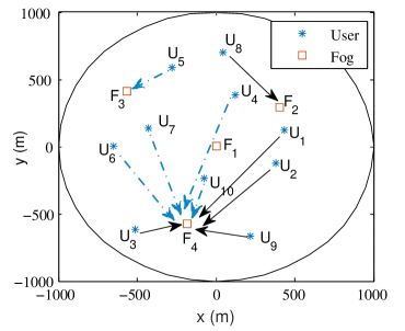
Figure 3: UE-Fog association after convergence.

Figure 3 shows the corresponding UE-Fog association and the task distribution after convergence in Figure 2. The arrow, which starts from UE and ends up at fog node, means that the UE offloads its task via the connected fog node. In particular, the solid black line means that the computation is performed at the fog node, and the blue broken line means that the computation is done at the cloud. From the figure we have the following observations: First, the UE-Fog association is not solely determined by the distance; i.e., UEs may offload their tasks to the fog nodes with larger distance. For example, most of UEs offload tasks via the fourth fog node, because the fourth fog node has the most powerful communication and computation capability. Therefore, Algorithm 1 can adaptively assign the UE-Fog association according to the available communication and computation resources. Secondly, when looking into the UEs connected with the fourth fog node, we found that the fourth fog node tends to locally perform the computation for those UEs with relatively “easy” tasks, i.e., smaller $D_{k}$ and $B_{k}$ such as UE1, UE2 and UE3, and forward the “hard” tasks to the cloud such as UE4, UE6 and UE7. This is intuitively reasonable, since the latency of completing the hard tasks is dominated by the computation latency rather than the transmission latency.

In the second example, we study how the task’s complexity $D_{k}$ affects the latency. For simplicity, we assume that all the fog nodes have the same computation capacity $F_{\ell,\max}=200$ (Gflops/second) and the same fronthaul capacity $C_{\ell,\max}=200$ (Mbps); all the UEs have the same $B_{k}=60$ (Kbits) and $D_{k}$; the cloud’s computation capacity is $F_{C,\max}=2\times 10^{3}$ (Gflops/second). For comparison, we have included two heuristic UE-Fog association strategies, namely, the minimum distance-based association and the random association, under which all the tasks are offloaded to the connected fog nodes or the cloud, and the fog nodes or the cloud equally allocate their resources for the served UEs. The result is shown in Figure 4. From the figure, we see that the proposed Algorithm 1 attains the minimum latency among the compared methods. The minimum distance-based offloading strategy is better than the random one, but there is still a notable performance gap between the former and Algorithm 1. In addition, we see that for both random connection and minimum distance-based connection schemes, the fog node computation is slightly better than the cloud computation, because for low-complexity tasks the latency is dominated by the transmission latency and further offloading to the cloud could incur larger latency. Actually, for the proposed Algorithm 1 we see a similar trend. More specifically, we calculate the ratio of tasks that are computed at the fog nodes for Algorithm 1 under the same setting as Figure 4, and the result is shown in Table I. As seen, with the increase of the tasks’ complexity, Algorithm 1 adaptively assigns more tasks to the cloud.

TABLE I: Ratio of tasks computed at the fog nodes vs. $D_{k}$.

$D_{k}$ (Mflops)	55	60	65	70	75	80	85
Ratio (%)	97	91	79	55	30	20	17

In the third example, we study how the maximum latency changes with the increase of the fog nodes’ computation capacity $F_{\ell,\max}$. The simulation is basically the same as the last one, except that we increase $B_{k}=150$ (Kbits), and $D_{k}=200$ (Mflops). The result is shown in Figure 5. As expected, when the fog nodes’ computation capacity increases, the maximum latency of all the schemes decrease. In addition, for the two compared schemes, they prefer to perform the computation at the fog nodes when $F_{\ell,\max}$ exceeds 400 Gflops/sec, since in such a case the latency is dominated by the transmission. Similar to Figure 4, the performance of Algorithm 1 is still far better than the other two schemes for all the tested $F_{\ell,\max}$.

In the fourth example, we investigate the relationship between the number of users and the maximum latency for different offloading strategies. The number of users increases from 2 to 11 according to the setting in Figure 2, and the result is shown in Figure 6. We see that with the increase of UEs, the maximum latency of all the schemes increases, but at different speed. Particularly, the random association scheme is more sensitive to the number of UEs, due to the lack of optimization for the UE-Fog association. Also, the proposed Algorithm 1 yields the best performance among the compared offloading schemes.

V-B The Cooperative Offloading Case

In this subsection, we study the performance of the cooperative offloading scheme, and make a comparison with the previous non-cooperative offloading. In the first example, we compare the performance of the cooperative and non-cooperative offloading schemes, when the fog nodes’ computation capacity $F_{\ell,\max}$ increases. For simplicity, we assume that all the fog nodes have the same $F_{\ell,\max}$ and $F_{C,\max}=1.5\times 10^{3}$  (Gflops/sec), $C_{\ell,\max}=200$ (Mbps), $\forall~{}\ell\in{\cal L}$, $B_{k}=100$ (Kbits) and $D_{k}=200$ (Mflops), $\forall~{}k\in{\cal K}$. The result is shown in Figure 7. From the figure, we see that with the increase of $F_{\ell,\max}$, the maximum latency decreases consistently. In particular, for small-to-medium $F_{\ell,\max}$ the cooperative offloading attains smaller latency than the non-cooperative one. However, when the fog nodes’ computation capacity exceeds the cloud’s, i.e., $F_{\ell,\max}\geq 1.5\times 10^{3}$ (Gflops/sec), the non-cooperative offloading becomes better. This can be explained as follows: When fog nodes have sufficient computation resources, it would be more preferable to process the tasks at the fog nodes, rather than compress-and-forwarding the tasks to the cloud, because the latter may further incur latency due to the capacity-limited fronthaul links. To verify this, we tabulate the ratio of tasks computed at the fog nodes for the two offloading schemes in Table II. It can be seen that the non-cooperative offloading has more fog nodes participating in the computation. By contrast, the cooperative scheme tends to offload the task to the cloud, because the cooperative compress-and-forwarding can better exploit the transmission diversity to reduce the transmission latency as compared with the non-cooperative offloading. In addition, we see that the “Cooperative min. distance (cloud compute)” scheme is better than the “non-cooperative min. distance (fog compute)” scheme, even if the fog’s computation capability exceeds the cloud’s. This again demonstrates the advantage of cooperative transmission in reducing the transmission latency.

TABLE II: Ratio of tasks computed at the fog nodes vs. fog nodes’ computation capacity $F_{\ell,\max}$.

$\begin{subarray}{c}F_{\ell,\max}\\ (\times 100\,{\rm Gflops/sec})\end{subarray}$	3	6	9	12	15	18	21
$\begin{subarray}{c}{\rm Non-cooperative}\\ (\%)\end{subarray}$	90	100	100	100	100	100	100
$\begin{subarray}{c}{\rm Cooperative}\\ (\%)\end{subarray}$	21	37	50	61	73	76	79

In the second example, we investigate the effect of the task size $B_{k}$ on the latency. We assume that all the UEs have same $B_{k}$, and other simulation parameters are $F_{\ell,\max}=500$  (Gflops/sec), $F_{C,\max}=2\times 10^{3}$ (Gflops/sec), $C_{\ell,\max}=200$ (Mbps), $\forall~{}\ell\in{\cal L}$ and $D_{k}=300$ (Mflops), $\forall~{}k\in{\cal K}$. The result is shown in Figure 8. As expected, the latency increases with $B_{k}$, and the cooperative offloading is consistently better than the non-cooperative one for all the tested $B_{k}$. Interestingly, under the cooperative mode, even the minimum distance-based UE-Fog association scheme can outperform the non-cooperative offloading; similar observation can be seen in Figure 7 for $F_{\ell,\max}\leq 600$ (Gflops/sec). This demonstrates that the cooperative gain is important for reducing latency.

VI Conclusion

We have considered multiuser computation offloading in fog-radio access networks under both non-cooperative and cooperative offloading models. To guarantee the worst latency performance of all UEs, a joint communication and computation resource allocation problem is formulated as a min-max MINP. By leveraging the continuous reformulation, we have developed efficient inexact MM approach to the min-max problems. Simulation results have demonstrated that the proposed offloading schemes are much better than some heuristic ones, and that the cooperative offloading is generally better than the non-cooperative one, owing to the cooperative gain from multiple fog nodes in the fronthaul transmissions.

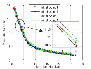
Figure 2: Convergence behavior of Algorithm 1 with different initializations.

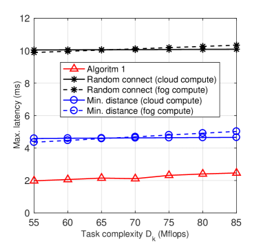
Figure 4: Maximum latency vs. $D_{k}$ (Mflops).

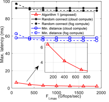
Figure 5: Maximum latency vs. fog nodes’ computation capacity $F_{\ell,\max}$.

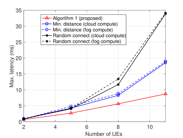
Figure 6: Maximum latency vs. number of UEs.

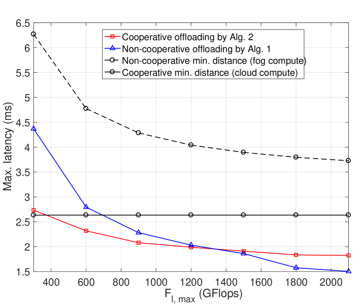
Figure 7: Maximum latency vs. fog nodes’ maximum computation capacity $F_{\ell,\max}$ for cooperative and non-cooperative offloading.

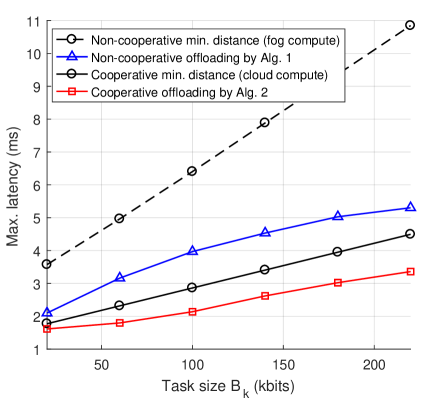
Figure 8: Maximum latency vs. the task size $B_{k}$.

Appendix A. Proof of Theorem 1

We first show that problem (6) is a relaxation of (5). Since the objective of (5) can be rewritten as $\alpha_{k,\ell}(1-\beta_{k})(\tau_{k,\ell}^{T}+\tau_{k,\ell}^{F})+\alpha_{k,\ell}\beta_{k}(\tau_{k,\ell}^{T}+\tau_{k,\ell}^{C})$, we set $\theta_{k,\ell}^{F}=\alpha_{k,\ell}(1-\beta_{k})$ and $\theta_{k,\ell}^{C}=\alpha_{k,\ell}\beta_{k}$. It is easy to see that $\theta_{k,\ell}^{F}$ and $\theta_{k,\ell}^{C}$ are both nonnegative, and $\sum_{\ell=1}^{L}\theta_{k,\ell}^{F}+\theta_{k,\ell}^{C}=\sum_{\ell=1}^{L}(\alpha_{k,\ell}(1-\beta_{k})+\alpha_{k,\ell}\beta_{k})=\sum_{\ell=1}^{L}\alpha_{k,\ell}=1,\forall~{}k$. Hence, the optimal solution of (5) is a feasible solution of (6). Next, we show that problem (6) has an optimal solution, which is also a feasible solution of (5), thereby establishing equivalence of the two problems. Suppose that $(\tilde{\theta}_{k,\ell}^{F},\tilde{\theta}_{k,\ell}^{C})$ is an optimal solution of (6) and $\tilde{\tau}_{k,\ell}^{X},~{}X\in\{T,F,C\},\forall~{}k,\ell$ is the corresponding latency calculated at the optimal solution. Without loss of generality, we assume $\tilde{\tau}_{k,\hat{\ell}}^{T}+\tilde{\tau}_{k,\hat{\ell}}^{F}\leq\tilde{\tau}_{k,{\ell}}^{T}+\tilde{\tau}_{k,{\ell}}^{F}$ and $\tilde{\tau}_{k,\hat{\ell}}^{T}+\tilde{\tau}_{k,\hat{\ell}}^{F}\leq\tilde{\tau}_{k,{\ell}}^{T}+\tilde{\tau}_{k,{\ell}}^{C}$ for all $\ell\neq\hat{\ell}$. In view of (6b) and (6c), it holds that

$$\sum_{\ell=1}^{L}\left(\tilde{\theta}_{k,\ell}^{F}(\tilde{\tau}_{k,\ell}^{T}+\tilde{\tau}_{k,\ell}^{F})+\tilde{\theta}_{k,\ell}^{C}(\tilde{\tau}_{k,\ell}^{T}+\tilde{\tau}_{k,\ell}^{C})\right)\geq\tilde{\tau}_{k,\hat{\ell}}^{T}+\tilde{\tau}_{k,\hat{\ell}}^{F},$$ (25)

That is, the choice of $\theta_{k,\hat{\ell}}^{F}=1$ and $\theta_{k,{\ell}}^{F}=\theta_{k,{\ell}}^{C}=0$ for all $\ell\neq\hat{\ell}$ is also optimal for (6). In addition, since the lower bound in (25) is independent of $\tilde{\tau}_{k,{\ell}}^{F},\forall~{}\ell\neq\hat{\ell}$ and $\tilde{\tau}_{k,{\ell}}^{C},\forall~{}\ell$, we can always set the communication and computational resources $f_{k,\ell}^{F}$, $C_{k,\ell}$ and $f_{k}^{C}$ appearing in $\tilde{\tau}_{k,{\ell}}^{F},\forall~{}\ell\neq\hat{\ell}$ and $\tilde{\tau}_{k,{\ell}}^{C},\forall~{}\ell$ to zero  without changing the optimal value $\tilde{\tau}_{k,\hat{\ell}}^{T}+\tilde{\tau}_{k,\hat{\ell}}^{F}$ of (6). It is easy to verify that this particularly constructed optimal solution is also feasible, and attains the same objective value $\tilde{\tau}_{k,\hat{\ell}}^{T}+\tilde{\tau}_{k,\hat{\ell}}^{F}$ for problem (5), if we set $\alpha_{k,\hat{\ell}}=1$, $\alpha_{k,{\ell}}=0,\forall~{}\ell\neq\hat{\ell}$ and $\beta_{k}=0$ in (6). This completes the proof.

Appendix B. Proof of Theorem 2

Let us define

$$\bm{x}\triangleq\{\bm{v}_{k},f_{k}^{C},\bm{\tau}_{k},\bm{\theta}_{k}R_{k,\ell},f_{k,\ell}^{F},C_{k,\ell}\}_{k,\ell},$$

$${\bm{y}}\triangleq\{\bm{u}_{k,\ell},w_{k,\ell}\}_{k,\ell},\quad\nu(\bm{x})\triangleq\max_{k\in\cal K}\Gamma_{k}(\bm{x}),\quad\Gamma_{k}(\bm{x})\triangleq\bm{\theta}_{k}^{T}\bm{\tau}_{k},$$

$$\tilde{\nu}(\bm{x},\bm{y};\bm{x}^{(t)})\triangleq\max_{k\in{\cal K}}\tilde{\Gamma}_{k}(\bm{x},\bm{y};\bm{x}^{(t)}),$$

$$\tilde{\Gamma}_{k}(\bm{x},\bm{y};\bm{x}^{(t)})\triangleq\frac{\|\bm{\theta}_{k}+\bm{\tau}_{k}\|^{2}}{2}-\left(\frac{1}{2}\|\bm{\theta}_{k}^{(t)}\|^{2}+\frac{1}{2}\|\bm{\tau}_{k}^{(t)}\|^{2}\right.$$

$$\left.+(\bm{\theta}_{k}^{(t)})^{T}(\bm{\theta}_{k}-\bm{\theta}_{k}^{(t)})+(\bm{\tau}_{k}^{(t)})^{T}(\bm{\tau}_{k}-\bm{\tau}_{k}^{(t)})\right).$$

Then, problem (12) can be concisely expressed as

$$\min_{\bm{x},\bm{y}} ~{}\tilde{\nu}(\bm{x},\bm{y};\bm{x}^{(t)})$$ (26)

$${\rm s.t.} ~{}\zeta_{k,\ell}(\bm{x},\bm{y})\leq 0,\forall~{}k,\ell,$$

$$~{}\psi_{i}(\bm{x})\leq 0,~{}i=1,\ldots,I,$$

where $\zeta_{k,\ell}(\bm{x},\bm{y})\triangleq R_{k,\ell}-f_{k,\ell}(\bm{u}_{k,\ell},w_{k,\ell},\bm{V})$ and $\psi_{i}(\bm{x})\leq 0$ denotes the constraints in (7c)-(7d) with $I$ being the total number of constraints. Without loss of generality, we assume $J^{(t)}=J$ for all $t$ in the following proof. With the above definitions and according to Algorithm 1, we have

$$\nu(\bm{x}^{(t)}) =\tilde{\nu}(\bm{x}^{(t)},\bm{y}^{(t)};\bm{x}^{(t)})$$ (27a)

$$=\tilde{\nu}(\bm{x}^{(t_{0})},\bm{y}^{(t_{0})};\bm{x}^{(t)})$$ (27b)

$$\geq\tilde{\nu}(\bm{x}^{(t_{1})},\bm{y}^{(t_{1})};\bm{x}^{(t)})$$ (27c)

$$\vdots$$

$$\geq\tilde{\nu}(\bm{x}^{(t_{J})},\bm{y}^{(t_{J})};\bm{x}^{(t)})$$ (27d)

$$\geq\nu(\bm{x}^{(t_{J})})$$ (27e)

$$=\nu(\bm{x}^{(t+1)})$$ (27f)

where (27a) follows from the definitions of $\nu$ and $\tilde{\nu}$; (27b) is because $\bm{x}^{(t)}$ is chosen as initialization of $\bm{x}^{(t_{0})}$; (27c) follows from the descent property of block-coordinate minimization; (27e) is because $\tilde{\nu}$ majorizes $\nu(\bm{x})$; (27f) follows from the definition of $\bm{x}^{t+1}$ in Algorithm 1. Therefore, the iterates $\{\bm{x}^{(t)}\}_{t}$ generated by Algorithm 1 yield a non-increasing objective values for problem (7). Since problem (7) is lower bounded below, by monotone convergence theorem, $\nu(\bm{x}^{(t)})$ must converge to some finite value, i.e.,

$$\lim_{t\rightarrow\infty}\nu(\bm{x}^{(t)})=\nu^{\star}>-\infty.$$

From (27a)-(27f), we also have

$$\lim_{t\rightarrow\infty}\tilde{\nu}(\bm{x}^{(t)},\bm{y}^{(t)};\bm{x}^{(t)})=\nu^{\star}.$$ (28)

Consider a converging subsequence $(\bm{x}^{(t_{j})},\bm{y}^{(t_{j})})_{j}$ of $(\bm{x}^{(t)},\bm{y}^{(t)})_{t}$ such that

$$\lim_{j\rightarrow\infty}(\bm{x}^{(t_{j})},\bm{y}^{(t_{j})})=(\bar{\bm{x}},\bar{\bm{y}}).$$

Now, by taking limit along the converging subsequence $({\bm{x}}^{(t_{j})},{\bm{y}}^{(t_{j})})_{j}$ on both sides of (28), we get

$$\tilde{\nu}(\bar{\bm{x}},\bar{\bm{y}};\bar{\bm{x}})=\nu^{\star}.$$ (29)

From the descent property in (27), we also have

$$\tilde{\nu}({\bm{x}},{\bm{y}}^{(t_{j})};{\bm{x}}^{(t_{j})})\geq\nu^{\star},~{}~{}\forall~{}\bm{x}\in{\cal F}(\bm{y}^{(t_{j})}),$$ (30)

where ${\cal F}(\bm{y}^{(t_{j})})$ denotes the feasible set of problem (26) when fixing $\bm{y}=\bm{y}^{(t_{j})}$. By taking limit along the converging subsequence $({\bm{x}}^{(t_{j})},{\bm{y}}^{(t_{j})})$ on both sides of (30), we get

$$\tilde{\nu}({\bm{x}},\bar{\bm{y}};\bar{\bm{x}})\geq\nu^{\star},\quad\forall~{}{\bm{x}}\in{\cal F}(\bar{\bm{y}})$$ (31)

Combining (29) and (31), we obtain the following key inequality:

$$\tilde{\nu}({\bm{x}},\bar{\bm{y}};\bar{\bm{x}})\geq\tilde{\nu}(\bar{\bm{x}},\bar{\bm{y}};\bar{\bm{x}}),\quad\forall~{}{\bm{x}}\in{\cal F}(\bar{\bm{y}}).$$ (32)

On the other hand, since ${\bm{y}}^{(t_{0})}$ is obtained by minimizing problem (26) with fixed ${\bm{x}}^{(t_{0})}$, we have

$$\tilde{\nu}({\bm{x}}^{(t_{0})},{\bm{y}}^{(t_{0})};{\bm{x}}^{(t)})\leq\tilde{\nu}({\bm{x}}^{(t_{0})},{\bm{y}};{\bm{x}}^{(t)}),~{}\forall~{}\bm{y}$$ (33)

Again, by taking limit along the converging subsequence $(\bm{x}^{(t_{j})},{\bm{y}}^{(t_{j})})_{j}$ on both sides of (33), we get another key inequality

$$\tilde{\nu}(\bar{\bm{x}},{\bm{y}};\bar{\bm{x}})\geq\tilde{\nu}(\bar{\bm{x}},\bar{\bm{y}};\bar{\bm{x}}),\quad\forall~{}\bm{y}.$$ (34)

Next, we will complete the proof by exploiting the two key inequalities in (32) and (34). Specifically, the inequality (32) implies that $\bar{\bm{x}}$ is an optimal solution for the following problem:

$$\min_{\bm{x}} ~{}\tilde{\nu}(\bm{x},\bar{\bm{y}};\bar{\bm{x}})$$ (35)

$${\rm s.t.} ~{}\zeta_{k,\ell}(\bm{x},\bar{\bm{y}})\leq 0,\forall~{}k,\ell,$$

$$~{}\psi_{i}(\bm{x})\leq 0,~{}i=1,\ldots,I.$$

Hence, $\bar{\bm{x}}$ must satisfy the KKT conditions of problem (35), which are listed below.

$$\bm{0}\in\partial_{\bm{x}}\tilde{\nu}(\bar{\bm{x}},\bar{\bm{y}};\bar{\bm{x}})+\textstyle\sum_{k,\ell}\kappa_{k,\ell}\nabla_{\bm{x}}\zeta_{k,\ell}(\bar{\bm{x}},\bar{\bm{y}})+\textstyle\sum_{i}\eta_{i}\nabla_{\bm{x}}\psi_{i}(\bar{\bm{x}})$$ (36)

$$\kappa_{k,\ell}\zeta_{k,\ell}(\bar{\bm{x}},\bar{\bm{y}})=0,$$

$$\eta_{i}\psi_{i}(\bar{\bm{x}})=0,$$

$$\zeta_{k,\ell}(\bar{\bm{x}},\bar{\bm{y}})\leq 0,~{}\forall~{}k,\ell,$$

$$\psi_{i}(\bar{\bm{x}})\leq 0,~{}\forall~{}i,$$

$$\kappa_{k,\ell}\geq 0,\quad\eta_{i}\geq 0,~{}\forall~{}k,\ell,i,$$

where $\kappa_{k,\ell}$ and $\eta_{i}$ are Lagrangian multipliers; $\partial_{\bm{x}}\tilde{\nu}$ denotes the subdifferential of $\tilde{\nu}$. Moreover, the inequality (34) implies that $\bar{\bm{y}}$ is an optimal solution of problem (26) for fixed $\bar{\bm{x}}$. Recall that for fixed $\bm{x}$, the optimal $\bm{y}$ can be uniquely computed in closed form by (13). Therefore, the optimal $\bar{\bm{y}}$ of problem (26) takes the form of (13) (with $\bm{V}$ replaced by $\bar{\bm{V}}$). Now, by substituting this specific $\bar{\bm{y}}$ into $\zeta_{k,\ell}(\bar{\bm{x}},\bar{\bm{y}})$, one can easily verify that the following holds:

$$\zeta_{k,\ell}(\bar{\bm{x}},\bar{\bm{y}}) =R_{k,\ell}-\phi_{k,\ell}(\bar{\bm{x}})$$ (37)

$$\nabla_{\bm{x}}\zeta_{k,\ell}(\bar{\bm{x}},\bar{\bm{y}}) =\nabla_{\bm{x}}\phi_{k,\ell}(\bar{\bm{x}}),$$

where $\phi_{k,\ell}$ is defined in (7). Notice that we have used Danskin’s theorem [61] to obtain the second equation in (37). By substituting (37) into (36), we almost obtain the KKT conditions of problem (7), except for one remaining issue to verify, i.e., $\partial_{\bm{x}}\tilde{\nu}(\bar{\bm{x}},\bar{\bm{y}};\bar{\bm{x}})=\partial_{\bm{x}}{\nu}(\bar{\bm{x}})$. This can be shown as follows. Notice that

$$\partial_{\bm{x}}\tilde{\nu}(\bar{\bm{x}},\bar{\bm{y}};\bar{\bm{x}})= {\rm Conv}\{\cup_{k\in\cal A}\nabla_{\bm{x}}\tilde{\Gamma}_{k}(\bar{\bm{x}},\bar{\bm{y}};\bar{\bm{x}})\}$$ (38)

$$= {\rm Conv}\{\cup_{k\in\cal A}\nabla_{\bm{x}}\Gamma_{k}(\bar{\bm{x}})\}$$

$$= \partial_{\bm{x}}{\nu}(\bar{\bm{x}})$$

where ${\rm Conv}\{\cdot\}$ denotes the convex hull, and ${\cal A}$ represents the set of active indices satisfying $\tilde{\Gamma}_{k}(\bar{\bm{x}},\bar{\bm{y}};\bar{\bm{x}})=\tilde{\nu}(\bar{\bm{x}},\bar{\bm{y}};\bar{\bm{x}})$. The second equality in (38) is due to the fact that $\tilde{\Gamma}_{k}({\bm{x}},\bar{\bm{y}};\bar{\bm{x}})$ is the tight approximation of $\Gamma_{k}({\bm{x}})$ up to first order at the point $\bm{x}=\bar{\bm{x}}$. This completes the proof.

References

- [1] M. Chiang and T. Zhang, “Fog and IoT: An overview of research opportunities,” IEEE Internet of Things Journal, vol. 3, no. 6, pp. 854–864, Dec. 2016.
- [2] M. Peng, S. Yan, K. Zhang, and C. Wang, “Fog-computing-based radio access networks: Issues and challenges,” IEEE Network, vol. 30, no. 4, pp. 46–53, July 2016.
- [3] F. Bonomi, R. Milito, J. Zhu, and S. Addepalli, “Fog computing and its role in the internet of things,” in Proc. ACM SIGCOMM Workshop on Mobile Cloud Computing, 2012, pp. 13–16.
- [4] P. Mach and Z. Becvar, “Mobile edge computing: A survey on architecture and computation offloading,” IEEE Communications Surveys Tutorials, vol. 19, no. 3, pp. 1628–1656, 3rd Quart. 2017.
- [5] M. Maray and J. Shuja, “Computation offloading in mobile cloud computing and mobile edge computing: Survey, taxonomy, and open issues,” Mobile Information Systems, vol. 2022, pp. 1–17, 2022.
- [6] S. Nayak, R. Patgiri, L. Waikhom, and A. Ahmed, “A review on edge analytics: Issues, challenges, opportunities, promises, future directions, and applications,” Digital Communications and Networks, 2022. [Online]. Available: https://www.sciencedirect.com/science/article/pii/S2352864822002255
- [7] K. Sadatdiynov, L. Cui, L. Zhang, J. Z. Huang, S. Salloum, and M. S. Mahmud, “A review of optimization methods for computation offloading in edge computing networks,” Digital Communications and Networks, 2022. [Online]. Available: https://www.sciencedirect.com/science/article/pii/S2352864822000244
- [8] M.-R. Ra, A. Sheth, L. Mummert, P. Pillai, D. Wetherall, and R. Govindan, “Odessa: Enabling interactive perception applications on mobile devices,” in Proc. 9th Int. Conf. Mobile Syst., Appl., Services, July 2011, pp. 43–56.
- [9] W. Zhang, Y. Wen, K. Guan, D. Kilper, H. Luo, and D. O. Wu, “Energy-optimal mobile cloud computing under stochastic wireless channel,” IEEE Trans. Wireless Commun., vol. 12, no. 9, pp. 4569–4581, Sep. 2013.
- [10] W. Zhang, Y. Wen, and D. O. Wu, “Collaborative task execution in mobile cloud computing under a stochastic wireless channel,” IEEE Trans. Wireless Commun., vol. 14, no. 1, pp. 81–93, Jan. 2015.
- [11] X. Chen, Y. Cai, Q. Shi, M. Zhao, and G. Yu, “Energy-efficient resource allocation for latency-sensitive mobile edge computing,” in IEEE VTC-Fall, Aug. 2018, pp. 1–5.
- [12] X. Lyu, H. Tian, W. Ni, Y. Zhang, P. Zhang, and R. Liu, “Energy-efficient admission of delay-sensitive tasks for mobile edge computing,” IEEE Trans. Commun., vol. 66, no. 6, pp. 2603–2616, June 2018.
- [13] F. Wang, J. Xu, X. Wang, and S. Cui, “Joint offloading and computing optimization in wireless powered mobile-edge computing systems,” IEEE Trans. Wireless Commun., vol. 17, no. 3, pp. 1784–1797, Mar. 2018.
- [14] Q. Liu, T. Han, and N. Ansari, “Joint radio and computation resource management for low latency mobile edge computing,” in IEEE Globecom, Dec. 2018, pp. 1–7.
- [15] Y. C. J. Ren, G. Yu and Y. He, “Latency optimization for resource allocation in mobile-edge computation offloading,” IEEE Trans. Wireless Commun., vol. 17, no. 8, pp. 5506–5519, Aug. 2018.
- [16] J. Du, L. Zhao, X. Chu, F. Yu, J. Feng, and C.-L. I, “Enabling low-latency applications in LTE-A based mixed fog/cloud computing systems,” IEEE Trans. Veh. Tech., vol. 68, no. 2, pp. 1757–1771, Feb. 2019.
- [17] U. Saleem, Y. Liu, S. Jangsher, X. Tao, and Y. Li, “Latency minimization for D2D-enabled partial computation offloading in mobile edge computing,” IEEE Transactions on Vehicular Technology, vol. 69, no. 4, pp. 4472–4486, 2020.
- [18] Z. Kuang, Z. Ma, Z. Li, and X. Deng, “Cooperative computation offloading and resource allocation for delay minimization in mobile edge computing,” Journal of Systems Architecture, vol. 118, p. 102167, 2021. [Online]. Available: https://www.sciencedirect.com/science/article/pii/S1383762121001181
- [19] Y. Li, T. Wang, Y. Wu, and W. Jia, “Optimal dynamic spectrum allocation-assisted latency minimization for multiuser mobile edge computing,” Digital Communications and Networks, vol. 8, no. 3, pp. 247–256, 2022.
- [20] T. X. Tran and D. Pompili, “Joint task offloading and resource allocation for multi-server mobile-edge computing networks,” IEEE Trans. Veh. Tech., vol. 68, no. 1, pp. 856–868, Jan. 2019.
- [21] J. Du, L. Zhao, J. Feng, and X. Chu, “Computation offloading and resource allocation in mixed fog/cloud computing systems with min-max fairness guarantee,” IEEE Trans. Commun., vol. 66, no. 4, pp. 1594–1608, Apr. 2018.
- [22] M.-H. Chen, M. Dong, and B. Liang, “Resource sharing of a computing access point for multi-user mobile cloud offloading with delay constraints,” IEEE Trans. Mobile Comput., vol. 17, no. 12, pp. 2868–2881, Dec. 2018.
- [23] Y. Liu, F. Yu, X. Li, H. Ji, and C.-M. Leung, “Distributed resource allocation and computation offloading in fog and cloud networks with non-orthogonal multiple access,” IEEE Trans. Veh. Tech., vol. 67, no. 12, pp. 12 137–12 151, Dec. 2018.
- [24] S. Liu, Y. Yu, L. Guo, P. L. Yeoh, B. Vucetic, and Y. Li, “Adaptive delay-energy balanced partial offloading strategy in mobile edge computing networks,” Digital Communications and Networks, 2022. [Online]. Available: https://www.sciencedirect.com/science/article/pii/S2352864822001225
- [25] T. Chen, Q. Ling, Y. Shen, and G. Giannakis, “Heterogeneous online learning for “thing-adaptive” fog computing in IoT,” IEEE Internet Things J., vol. 5, no. 6, pp. 4328–4341, Dec. 2018.
- [26] Y. Dong, X. Jiang, H. Zhou, Y. Lin, and Q. Shi, “SR2CNN: Zero-shot learning for signal recognition,” IEEE Transactions on Signal Processing, vol. 69, pp. 2316–2329, 2021.
- [27] Y. Lin, Y. Tu, Z. Dou, L. Chen, and S. Mao, “Contour Stella image and deep learning for signal recognition in the physical layer,” IEEE Transactions on Cognitive Communications and Networking, vol. 7, no. 1, pp. 34–46, 2021.
- [28] Y. Tu, Y. Lin, and H. Zha, “Large-scale real-world radio signal recognition with deep learning,” Chinese Journal of Aeronautics, vol. 35, no. 9, pp. 35–48, Sep. 2022.
- [29] Y. Li, S. Xia, M. Zheng, B. Cao, and Q. Liu, “Lyapunov optimization-based trade-off policy for mobile cloud offloading in heterogeneous wireless networks,” IEEE Transactions on Cloud Computing, vol. 10, no. 1, pp. 491–505, 2022.
- [30] S. Xia, Z. Yao, Y. Li, and S. Mao, “Online distributed offloading and computing resource management with energy harvesting for heterogeneous mec-enabled iot,” IEEE Transactions on Wireless Communications, vol. 20, no. 10, pp. 6743–6757, 2021.
- [31] Y. Li, H. Ma, L. Wang, S. Mao, and G. Wang, “Optimized content caching and user association for edge computing in densely deployed heterogeneous networks,” IEEE Transactions on Mobile Computing, vol. 21, no. 6, pp. 2130–2142, 2022.
- [32] D. R. Hunter and K. Lange, “A tutorial on MM algorithms,” The American Statistician, vol. 58, no. 12, pp. 30–37, 2004.
- [33] Q. Shi, M. Razaviyayn, Z.-Q. Luo, and C. He, “An iteratively weighted MMSE approach to distributed sum-utility maximization for a MIMO interfering broadcast channel,” IEEE Trans. Signal Process., vol. 59, no. 9, pp. 4331–4340, Sep. 2011.
- [34] S. Sardellitti, G. Scutari, and S. Barbarossa, “Joint optimization of radio and computational resources for multicell mobile-edge computing,” IEEE Trans. Signal Inf. Process. Netw., vol. 1, no. 2, pp. 89–103, Jun. 2015.
- [35] M. Salmani and T. N. Davidson, “Multiple access computational offloading with computation constraints,” in IEEE Workshop on Sig. Proc. Adv. in Wireless Commun., July 2017, pp. 385–389.
- [36] S. Mostafa, C. W. Sung, and Y. Guo, “Joint computation and communication resource allocation with NOMA and OMA offloading for multi-server systems in F-RAN,” IEEE Access, vol. 10, pp. 24 456–24 466, 2022.
- [37] T.-C. Chiu, W.-H. Chung, A.-C. Pang, Y.-J. Yu, and P.-H. Yen, “Ultra-low latency service provision in 5G fog-radio access networks,” in Proc. IEEE PIMRC, Sept. 2016.
- [38] A.-C. Pang, W.-H. Chung, T.-C. Chiu, and J. Zhang, “Latency-driven cooperative task computing in multi-user fog-radio access networks,” in IEEE 37th International Conference on Distributed Computing Systems, June 2017, pp. 615–624.
- [39] Y. Pan, H. Jiang, H. Zhu, and J. Wang, “Latency minimization for task offloading in hierarchical fog-computing c-ran networks,” in ICC 2020 - 2020 IEEE International Conference on Communications (ICC), 2020, pp. 1–6.
- [40] J. Tan, T.-H. Chang, K. Guo, and T. Quek, “Robust computation offloading in fog radio access network with fronthaul compression,” IEEE Trans. Wireless Commun., vol. 20, no. 10, pp. 6506–6521, Oct. 2021.
- [41] Z. Zhao, S. Bu, T. Zhao, Z. Yin, M. Peng, Z. Ding, and T. Q. S. Quek, “On the design of computation offloading in fog radio access networks,” IEEE Transactions on Vehicular Technology, vol. 68, no. 7, pp. 7136–7149, 2019.
- [42] K. Guo, M. Sheng, T. Q. S. Quek, and Z. Qiu, “Task offloading and scheduling in fog ran: A parallel communication and computation perspective,” IEEE Wireless Communications Letters, vol. 9, no. 2, pp. 215–218, 2020.
- [43] Q. D. La, M. V. Ngo, T. Q. Dinh, T. Q. Quek, and H. Shin, “Enabling intelligence in fog computing to achieve energy and latency reduction,” Digital Communications and Networks, vol. 5, no. 1, pp. 3–9, 2019.
- [44] Y. Ma, H. Wang, J. Xiong, J. Diao, and D. Ma, “Joint allocation on communication and computing resources for fog radio access networks,” IEEE Access, vol. 8, pp. 108 310–108 323, 2020.
- [45] Z. Zhao, C. Feng, H. H. Yang, and X. Luo, “Federated-learning-enabled intelligent fog radio access networks: Fundamental theory, key techniques, and future trends,” IEEE Wireless Communications, vol. 27, no. 2, pp. 22–28, 2020.
- [46] G. M. S. Rahman, T. Dang, and M. Ahmed, “Deep reinforcement learning based computation offloading and resource allocation for low-latency fog radio access networks,” Intelligent and Converged Networks, vol. 1, no. 3, pp. 243–257, 2020.
- [47] H. Lee, J. Kim, and S.-H. Park, “Learning optimal fronthauling and decentralized edge computation in fog radio access networks,” IEEE Transactions on Wireless Communications, vol. 20, no. 9, pp. 5599–5612, 2021.
- [48] F. Jiang, X. Zhu, and C. Sun, “Double dqn based computing offloading scheme for fog radio access networks,” in 2021 IEEE/CIC International Conference on Communications in China (ICCC), 2021, pp. 1131–1136.
- [49] L. Zhang, Y. Jiang, F.-C. Zheng, M. Bennis, and X. You, “Computation offloading and resource allocation in f-rans: A federated deep reinforcement learning approach,” in 2022 IEEE International Conference on Communications Workshops (ICC Workshops), 2022, pp. 97–102.
- [50] M. Xu, Z. Zhao, M. Peng, Z. Ding, T. Q. S. Quek, and W. Bai, “Performance analysis of computation offloading in fog-radio access networks,” in ICC 2019 - 2019 IEEE International Conference on Communications (ICC), 2019, pp. 1–6.
- [51] J. Jijin, B.-C. Seet, and P. H. J. Chong, “Performance analysis of opportunistic fog based radio access networks,” IEEE Access, vol. 8, pp. 225 191–225 200, 2020.
- [52] Q. Ren, K. Liu, and L. Zhang, “Multi-objective optimization for task offloading based on network calculus in fog environments,” Digital Communications and Networks, 2021. [Online]. Available: https://www.sciencedirect.com/science/article/pii/S2352864821000729
- [53] T. H. L. Dinh, M. Kaneko, E. H. Fukuda, and L. Boukhatem, “Energy efficient resource allocation optimization in fog radio access networks with outdated channel knowledge,” IEEE Transactions on Green Communications and Networking, vol. 5, no. 1, pp. 146–159, 2021.
- [54] X. Liu, H. Zhang, K. Long, A. Nallanathan, and V. C. M. Leung, “Energy efficient user association, resource allocation and caching deployment in fog radio access networks,” IEEE Transactions on Vehicular Technology, vol. 71, no. 2, pp. 1846–1856, 2022.
- [55] Y. Jiang, C. Wan, M. Tao, F.-C. Zheng, P. Zhu, X. Gao, and X. You, “Analysis and optimization of fog radio access networks with hybrid caching: Delay and energy efficiency,” IEEE Transactions on Wireless Communications, vol. 20, no. 1, pp. 69–82, 2021.
- [56] A. Bani-Bakr, M. N. Hindia, K. Dimyati, Z. B. Zawawi, and T. F. Tengku Mohmed Noor Izam, “Caching and multicasting for fog radio access networks,” IEEE Access, vol. 10, pp. 1823–1838, 2022.
- [57] Z. Wang, Y. Sun, and S. Yuan, “Intelligent radio access networks: architectures, key techniques, and experimental platforms,” Front Inform. Technol. Electron. Eng., vol. 23, pp. 5–18, 2022.
- [58] M. Grant and S. Boyd, “CVX: Matlab software for disciplined convex programming, version 2.1,” http://cvxr.com/cvx, Mar. 2014.
- [59] Y. Zhou and W. Yu, “Fronthaul compression and transmit beamforming optimization for multi-antenna uplink C-RAN,” IEEE Trans. Sig. Process., vol. 64, no. 16, pp. 4138–4151, Aug. 2016.
- [60] Q. Li, M. Hong, H.-T. Wai, Y. Liu, W.-K. Ma, and Z.-Q. Luo, “Transmit solutions for MIMO wiretap channels using alternating optimization,” IEEE J. Selected Areas Commun., vol. 31, no. 9, pp. 1714–1727, Sep. 2013.
- [61] D. Bertsekas, Nonlinear Programming. Belmont, MA: Athena Scientific, 1999.