Early Structure Formation in $\Lambda$PBH Cosmologies

Abstract

Cold dark matter (CDM) could be composed of primordial black holes (PBH) in addition to or instead of more orthodox weakly interacting massive particle dark matter (PDM). We study the formation of the first structures in such $\Lambda$PBH cosmologies using $N$-body simulations evolved from deep in the radiation era to redshift 99. When PBH are only a small component of the CDM, they are clothed by PDM to form isolated halos. On the other hand, when PBH make most of the CDM, halos can also grow via clustering of many PBH. We find that the halo mass function is well modelled via Poisson statistics assuming random initial conditions. We quantify the nonlinear velocities induced by structure formation and find that they are too small to significantly impact CMB constraints. A chief challenge is how best to extrapolate our results to lower redshifts relevant for some observational constraints.

I Introduction

Despite overwhelming evidence for cold dark matter (CDM), we have no knowledge of what it is composed of. The prevailing candidate has been a Weakly Interacting Massive Particle (WIMP) which freezes out in the early Universe as a cold relic (Jungman et al., 1996). However, there has been neither direct nor indirect detection of such a WIMP. Furthermore, the predictions of a completely cold species is in potential tension with some observations of small-scale structure (Bullock and Boylan-Kolchin, 2017). Alternative particle explanations of CDM include warm (Dodelson and Widrow, 1994), fuzzy (Hu et al., 2000) and axion dark matter (Marsh, 2016), none of which have been detected.

It is also possible to consider non-particle based candidates for CDM, of which primordial black holes (PBH) are a long-studied favorite (Zel’dovich and Novikov, 1967; Hawking, 1971; Carr and Hawking, 1974) (see, e.g., (Carr et al., 2016; García-Bellido, 2017) for more modern discussions). Detections by LIGO of the merger of black hole binaries with masses of order $\sim 10~{}M_{\odot}$ (Abbott et al., 2016a, b, 2017a, 2017b, 2017c) have led to the suggestion that the coalescing black holes may have been primordial and could make up (at least part of) the CDM (Bird et al., 2016; Clesse and García-Bellido, 2017; Sasaki et al., 2016). Even if PBH do not make all of the dark matter, the possibility of both WIMP-like particles (which we will generically call PDM for “Particle Dark Matter”) and PBH coexisting and interacting gravitationally will have novel phenomenology. In this paper, we perform numerical calculations of mixed PBH-PDM dark matter, and examine their nonlinear dynamics down to redshift 99.

In addition to being a bona fide dark matter candidate, PBH can provide a window onto the initial conditions in the Universe. On large scales, the initial power spectrum has been precisely constrained to be nearly scale invariant with overdensities of $\lesssim 10^{-4}$ (Planck Collaboration et al., 2016). However, the power spectrum on ultra small scales is only poorly constrained (see, e.g., (Jeong et al., 2014; Nakama et al., 2014)), and could be significantly larger. Enhanced initial overdensities on small scales can yield very rich phenomena. If they are greater than $\gtrsim 10^{-3}$ then standard adiabatic PDM perturbations form bound nonlinear structures almost immediately at matter radiation equality (Ricotti and Gould, 2009). Such structures were thought to be extremely dense, and so called ultracompact minihalos (UCMH), but recent numerical work has indicated that this is not the case due to frequent mergers (Gosenca et al., 2017; Delos et al., 2018; Sten Delos et al., 2018). An alternative way to produce early structure formation is a strong blue-tilt to the power spectrum (Hirano et al., 2015). Larger perturbations can form PDM “clumps” in radiation domination (Berezinsky et al., 2010) and even cause shocks in the radiation fluid (Pen and Turok, 2016). Increasing the primordial amplitude even further, $\gtrsim 10^{-1}$, will cause PBH to form (Green et al., 2004). Such PBH form regardless of whether there is some alternate form of PDM, and so are their own unique CDM candidate.

On sufficiently large scales, we expect the PBH density field to follow the standard adiabatic perturbations. However, on small enough scales, the discrete nature of PBH becomes important. If PBH make up only a small fraction of the CDM then we expect them to be clothed by a large amount of PDM, but not interact with any other PBH. This allows for analytic treatments of accretion, e.g., (Ricotti, 2007; Mack et al., 2007; Ricotti and Gould, 2009; Rice and Zhang, 2017; Lacki and Beacom, 2010; Eroshenko, 2016), and the resulting halos (HL) are expected to be similar to the theorized UCMH with a very steep density profile (Bertschinger, 1985). In the opposing limit, when PBH are the entirety of the CDM, the large-scale behaviour is still the adiabatic growing mode, but on small scales the random locations of PBH introduces a shot noise in their density (Afshordi et al., 2003). These two limits have respectively been called the “seed” and “Poisson” limits and have ramifications for supermassive black hole formation (Carr and Silk, 2018). Intermediate cases, on the other hand, are difficult to study analytically due to the competition of PBH in accreting PDM and PBH-PBH interactions.

It is important to understand these highly nonlinear dynamics in order to make accurate constraints on the amount of PBH. For instance, gravitational constraints which assume a uniform density, such as those from microlensing (Alcock et al., 2000) and dynamical heating (Brandt, 2016) could be affected if PBH become highly clustered at late times (e.g. Metcalf and Silk (1996)). The fact that PBH could have a steep PDM profile could affect potential constraints coming from pulsar timing (Schutz and Liu, 2017) where the associated PDM halo could also induce Shapiro delay (Clark et al., 2016, 2017). Such a steep PDM profile could also cause PDM annihilation to be observed (Lacki and Beacom, 2010), although this assumes a specific form for the PDM. Furthermore, Poisson fluctuations can cause PBH binaries to form in the early Universe (Nakamura et al., 1997) which could then merge and be detected by LIGO (Ali-Haïmoud et al., 2017; Raidal et al., 2017). While analytic estimates suggest that the tidal field on these binaries is insufficient to disrupt them Ioka et al. (1998); Ali-Haïmoud et al. (2017), it is possible that nonlinear effects could affect this conclusion Raidal et al. (2018). Such constraints come from astrophysical observations at late times in the local Universe. The CMB also provides constraints on PBH abundances Miller (2000); Miller and Ostriker (2001); Ricotti et al. (2008), and is sensitive to relative motion between PBH and gas in the Universe which will include a nonlinear component (Ali-Haïmoud and Kamionkowski, 2017; Poulin et al., 2017).

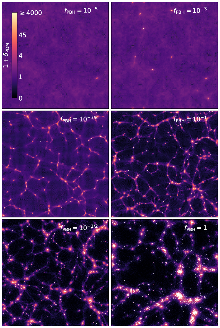
Figure 1: The matter field at $z=99$ for various PBH fractions. The PDM density field is represented by the colormap with white points indicating PBH locations. The slice width is 1/16 the box size, just under 2 kpc/$h$.

To correctly understand such nonlinear dynamics we must utilize numerical simulations. In this work, we develop $N$-body simulations which evolve both PDM and PBH particles and analyze the resulting halo characteristics. We focus on the scenario where $M_{\rm PBH}=20~{}h^{-1}M_{\odot}$ but vary the relative fraction of PBH to PDM. We illustrate our results in Fig. 1 which shows the PDM density fields alongside points to indicate where PBH and halos are. The differences between “$\Lambda$PDM” (top left panel) and “$\Lambda$PBH” (bottom right panel) are quite dramatic! In the next section we describe how these simulations were performed. We then show our results for PDM clustering around PBH, the halo mass function, and the distribution of PBH velocities, which we argue do not significantly affect CMB constraints. Lastly, we conclude by discussing how these simulations can next be used to improve constraints based on primordial PBH binaries and also how they may affect the formation of first stars at cosmic dawn.

II Cosmology

II.1 Background cosmology

Before describing the computations in more detail, it is worth going through the cosmic inventory to give an overview of how we treat different components and values of cosmological parameters used in the simulations. Throughout this work, we use cosmological parameters consistent with Planck results (Planck Collaboration et al., 2016).

$\bullet$ Matter – The matter sector consists of PBH (which for simplicity we assume to all have the same mass $M_{{\rm PBH}}$), PDM and baryons and contributes $\Omega_{m}=\Omega_{c}+\Omega_{b}$ to the energy density. The PBH and PDM contribute $\Omega_{c}=0.26$ to the energy density and their individual contributions are parameterized via $f_{{\rm PBH}}$ such that $\Omega_{{\rm PBH}}=f_{{\rm PBH}}\Omega_{c}$ and $\Omega_{{\rm PDM}}=(1-f_{{\rm PBH}})\Omega_{c}$. The baryons contribute $\Omega_{b}=0.05$. We do not include hydrodynamics in our simulations and therefore treat the baryons as an unclustered species, adding a constant $\Omega_{b}/\Omega_{m}$ to the grid. This is a very good approximation at early times when baryons are coupled to photons via Compton scattering, but becomes progressively worse as they begin to catch up to the PDM and cluster around PBH. For the purely gravitational effects of primary interest in this work, the neglect of baryon clustering leads to errors of order $\Omega_{b}/\Omega_{m}$.

$\bullet$ Radiation – Neutrinos and photons, collectively radiation, dominate the energy budget in the early stages of the Universe. Their energy density is parameterized by the redshift of matter-radiation equality, $z_{\rm eq}=3374$, such that $\Omega_{r}=\Omega_{m}/(1+z_{\rm eq})$. Photons and neutrinos are essentially free-streaming on the scales relevant to our simulations, so we assume they are homogeneous and only contribute to the expansion rate. We assume the neutrinos are massless, although this should have little effect on our results as they are largely relativistic at the times of interest.

$\bullet$ Dark Energy and Curvature – Dark energy takes up whatever is needed to have a flat, critical density Universe: $\Omega_{\Lambda}=1-\Omega_{r}-\Omega_{m}$. At the redshifts considered here, the dynamical effects of dark energy are completely negligible, although for definiteness we assume a standard cosmological constant.

The expansion of the Universe is therefore given by the standard Hubble equation:

$$H=\frac{d\ln a}{dt}=H_{0}\sqrt{\Omega_{\Lambda}+\Omega_{m}a^{-3}+\Omega_{r}a^{-4}}.$$ (1)

with $H_{0}=100~{}h~{}{\rm km/s/Mpc}$ with $h=0.67$, although the simulations are only sensitive to this value through the initial conditions.

II.2 Initial perturbations

The most natural way to form PBHs is through enhanced primordial curvature perturbations, collapsing into black holes upon horizon entry Carr (1975). The PBH mass depends on the initial overdensity, but is typically comparable to the mass-energy inside the Hubble radius at the time of collapse Niemeyer and Jedamzik (1998). The relationship between the scale $k_{*}$ at which the power spectrum is enhanced and the characteristic PBH mass is then Sasaki et al. (2018)

$$M_{\rm PBH}\approx 30~{}M_{\odot}\left(\frac{300~{}\textrm{kpc}^{-1}}{k_{*}}\right)^{2}.$$ (2)

For comparison, the comoving scales relevant to our simulations are $k\approx 0.15-38$ kpc^-1, as we will discuss in the next section. The smallest modes simulated are therefore only separated from the PBH scale by a factor of 8 or so.

For Gaussian initial conditions, the variance of curvature perturbations required to form PBHs is $\Delta^{2}\approx 0.03$ (see e.g. Germani and Musco (2019); Young et al. (2019) and references therein). The abundance of PBHs typically depends exponentially on $\Delta^{2}$, and conversely, the detailed amplitude only depends logarithmically on $f_{\rm PBH}$. It is therefore likely that the initial curvature perturbation is still rather large on the smallest scales we simulate. Ref. Byrnes et al. (2018) showed that, for primordial perturbations generated during single-field inflation, the steepest possible growth of the primordial curvature power spectrum (per $\ln k$) scales as $k^{4}$. Therefore, within single-field inflation, and neglecting non-Gaussianities, the existence of PBHs would require $\Delta^{2}\gtrsim 10^{-5}$ on the simulation grid scale, significantly larger than the amplitude on scales probed by CMB-anisotropy measurements, with $\Delta^{2}_{\rm CMB}\approx 2\times 10^{-9}$. On scales $k\lesssim 5$ kpc^-1, $\Delta^{2}\approx\Delta_{\rm CMB}^{2}$ is compatible with PBH formation (at least within the single-field, Gaussian approximation). Also note that upper limits on CMB spectral distortions imply that Chluba et al. (2012) $\Delta^{2}\lesssim 3\times 10^{-5}$ for $0.1\lesssim k~{}\textrm{kpc}\lesssim 5$.

For simplicity, we assume a primordial curvature power spectrum extrapolated from CMB scales, with a constant spectral index, i.e.

$$\Delta^{2}(k) =2.215\times 10^{-9}\left(\frac{k}{0.075~{}h/\textrm{kpc}}\right)^{-0.038}$$

$$=1.544\times 10^{-9}\left(\frac{k}{1~{}h/\textrm{kpc}}\right)^{-0.038}.$$ (3)

As we discussed above, on the smallest scales of our simulations, this is inconsistent with PBH formation in the case of single-field-inflation with Gaussian initial conditions. It may still be consistent with PBH formation for different sets of assumptions. Moreover, we do not expect this choice to affect any of our results; indeed, the initial adiabatic perturbations of PDM are quickly overwhelmed by isocurvature perturbations due to PBHs, as we will see later on.

We assume that the primordial PDM perturbations are adiabatic, as are PBH fluctuations on sufficiently large scales. On small enough scales, however, we assume PBHs are effectively randomly distributed Ali-Haïmoud (2018); Ballesteros et al. (2018); Desjacques and Riotto (2018). The variance of initial Poisson perturbations (per $\ln k$) takes the form

$$\Delta_{\rm PBH}^{2}(k)=(k/k_{*})^{3},$$ (4)

where $k_{*}$ is of order the inverse mean separation between PBHs:

$$k_{*}=\left(2\pi^{2}\overline{n}_{\rm bh}\right)^{1/3}\approx 4~{}h/\textrm{kpc}~{}f_{\rm PBH}^{1/3}\left(\frac{20~{}M_{\odot}/h}{M_{\rm PBH}}\right)^{1/3}.$$ (5)

On the $\sim$ kpc scales of our simulations, discreteness noise largely overwhelms the intrinsic adiabatic perturbations of PBHs.

III Methods

The $N$-body code used here is a modified version of CUBEP³M, a fast, massively parallel cosmological simulation code (Merz et al., 2005; Harnois-Déraps et al., 2013; Emberson et al., 2017). The addition of PBH builds off the neutrino integration described in (Inman et al., 2015; Emberson et al., 2017).

III.1 Simulation setup

For a given fraction $f_{\rm PBH}$ of CDM in PBH of mass $M_{{\rm PBH}}$, we need to select the optimal numerical parameters for our simulations. These parameters are the number of $N$-body particles used to evolve the PBH and PDM ($N_{{\rm PBH}}$ and $N_{\rm PDM}$, respectively) and the simulation box size $L$. Given the box size and number of particles, the $N$-body particle mass is then given by

$$m_{i}=278~{}h^{-1}M_{\odot}\left(h^{-1}\textrm{kpc}\right)^{-3}\Omega_{i}(L^{3}/N_{i}).$$ (6)

We are interested in studying the effects arising from the discreteness of PBH, and therefore set the PBH particle mass to the physical PBH mass, $m_{\rm PBH}=M_{\rm PBH}$. In contrast, it is virtually impossible to simulate individual PDM particles due to their large abundance; in that case, $N$-body particles represent, as is standard, chunks of phase-space. To maximize accuracy, we assign as large a number of PDM particles as allowed by computational resources. Our fiducial setup has $N_{\rm PDM}=N_{\rm fid}\equiv 2\times 256^{3}$. These considerations determine two combinations of the three parameters $(N_{\rm PBH},N_{\rm PDM},L)$. To determine the third, we enforce that the artificial Poisson noise from PDM $N$-body particles is subdominant to the physical Poisson fluctuations in the PBH abundance. Poisson noise is inversely proportional to the number of particles (for a fixed box size), so this criterion amounts to

$$\frac{(1-f_{\rm PBH})^{2}}{N_{\rm PDM}}\ll\frac{f_{\rm PBH}^{2}}{N_{\rm PBH}},$$ (7)

where the factors $(1-f_{\rm PBH})$ and $f_{\rm PBH}$ weigh the respective contributions to the total mass density perturbation. Using Eq. (6) with $m_{{\rm PBH}}=M_{\rm PBH}$, we rewrite this as

$$\left(\frac{L}{h^{-1}\textrm{kpc}}\right)^{3}\ll\frac{M_{{\rm PBH}}}{72~{}h^{-1}M_{\odot}}N_{{\rm PBH}}\frac{f_{\rm PBH}}{(1-f_{\rm PBH})^{2}}.$$ (8)

This limits the box size to

$$L \lesssim 200~{}h^{-1}\textrm{kpc}\left(\frac{M_{{\rm PBH}}}{20~{}h^{-1}M_{\odot}}\frac{N_{{\rm PDM}}}{N_{\rm fid}}\right)^{1/3}$$

$$\times\frac{f_{\rm PBH}^{1/3}}{(1-f_{\rm PBH})^{2/3}}.$$ (9)

Rather than adjusting $L$ for each value of $f_{\rm PBH}$, we choose to have a single box size, to facilitate comparisons between simulations. We pick $L=30~{}h^{-1}$ kpc for $M_{\rm PBH}=20~{}h^{-1}M_{\odot}$, which satisfies the criterion (9) for $f_{\rm PBH}\gtrsim 10^{-3}$. In simulations with lower $f_{\rm PBH}$, discreteness noise from PDM particles is less of an issue. Instead, we want the PDM halos that form around any PBH to be well resolved by many particles once the PDM halo mass becomes comparable to the PBH mass. This then implies that the mass ratio

$$\frac{m_{\rm PBH}}{m_{\rm PDM}}=\frac{f_{\rm PBH}}{1-f_{\rm PBH}}\frac{N_{\rm PDM}}{N_{\rm PBH}}$$ (10)

must be kept large to properly resolve the halo formation. As an example, our simulation with $f_{\rm PBH}=10^{-5}$ containing just a single PBH has a halo containing thousands of PDM particles, whereas the ratio of $N_{\rm PDM}/N_{\rm PBH}$ is only a few hundred for the simulation with $f_{\rm PBH}=1$. In practice, this limits the value of $f_{\rm PBH}$ to

$$f_{\rm PBH}\gg\frac{1}{1+\frac{N_{\rm PDM}}{N_{\rm PBH}}}$$ (11)

which for our choice of parameters implies $f_{\rm PBH}\gg N_{\rm PBH}/N_{\rm PDM}\geq 3\times 10^{-8}$.

With these parameters, the number of PBH in the simulation box is $N_{\rm PBH}=10^{5}f_{\rm PBH}$, and the mass of the PDM $N$-body particles is $m_{{\rm PDM}}\approx 0.058~{}h^{-1}M_{\odot}(1-f_{\rm PBH})$. For simulations with $f_{\rm PBH}=1$ where $m_{\rm PDM}=0$, we opt to still evolve the PDM particles as tracer particles, hence neglect PDM-PDM forces. We keep PDM particles in our $f_{\rm PBH}\rightarrow 1$ simulations as even a small fraction of PDM could have noticeable effects (for instance, if the PDM self annihilates (Lacki and Beacom, 2010; Adamek et al., 2019).

III.2 Initial Conditions

III.2.1 Large scales

In this section we focus on scales larger than the characteristic inter-PBH separation, $k\lesssim\overline{n}_{{\rm PBH}}^{1/3}$, so that we can treat PBHs as a quasi-homogeneous ideal pressureless fluid.

We assume that the primordial PDM perturbations (i.e. prior to horizon entry, and labelled by the superscript 0) are purely adiabatic on all scales, $\delta_{{\rm PDM}}^{0}=\delta_{\rm ad}^{0}$ and $\dot{\delta}_{{\rm PDM}}^{0}=\dot{\delta}_{\rm ad}^{0}$. We decompose the primordial PBH overdensity into an adiabatic piece and an uncorrelated isocurvature piece: $\delta_{\rm PBH}^{0}\equiv\delta_{\rm ad}^{0}+\delta_{\rm iso}^{0}$. The latter is due to the discreteness of PBHs, which prevents them from being distributed strictly adiabatically on small scales. It largely dominates over the adiabatic piece over all scales of our simulation. We assume that PBHs are formed with negligible velocities relative to the PDM, so that $\dot{\delta}_{{\rm PBH}}^{0}=\dot{\delta}_{{\rm PDM}}^{0}=\dot{\delta}_{\rm ad}^{0}$.

We define the total dark matter overdensity as $\delta_{c}\equiv(1-f_{\rm PBH})\delta_{\rm PDM}+f_{\rm PBH}\delta_{\rm PBH}$, and the difference field as $\delta_{-}\equiv\delta_{\rm PBH}-\delta_{\rm PDM}$. The PDM and PBH density fields are related to those through

$$\delta_{\rm PDM} =\delta_{c}-f_{\rm PBH}\delta_{-},$$ (12)

$$\delta_{\rm PBH} =\delta_{c}+(1-f_{\rm PBH})\delta_{-}.$$ (13)

The initial conditions for the total CDM perturbation are $\delta_{c}^{0}=\delta_{\rm ad}^{0}+f_{\rm PBH}\delta_{\rm iso}^{0}$, $\dot{\delta}_{c}^{0}=\dot{\delta}_{\rm ad}^{0}$. We denote by $T_{\rm ad}(a)$ and $T_{\rm iso}(a)$ the linear transfer functions of the adiabatic and CDM density isocurvature modes, respectively, both normalized to unity at $a\rightarrow 0$. The CDM overdensity at scale factor $a$ is then

$$\delta_{c}(a)=T_{\rm ad}(a)\delta_{\rm ad}^{0}+T_{\rm iso}(a)f_{\rm PBH}\delta_{\rm iso}^{0}.$$ (14)

Since both PDM and PBHs are cold fluids, they are subject to the same forces, and their (gauge-invariant) relative velocity decays as $1/a$. Having assumed a negligible primordial relative velocity, we conclude that it remains so at all times. As a consequence, the difference of the linearized continuity equations imply that $\delta_{-}=\delta_{-}^{0}=\delta_{\rm iso}^{0}$ is constant. Inserting Eq. (14) into Eqs. (12) and (13), we obtain

$$\delta_{\rm PDM}(a) =T_{\rm ad}(a)\delta_{\rm ad}^{0}+\left(T_{\rm iso}(a)-1\right)f_{\rm PBH}\delta_{\rm iso}^{0},$$ (15)

$$\delta_{\rm PBH}(a) =\delta_{\rm iso}^{0}+\delta_{{\rm PDM}}(a).$$ (16)

Both adiabatic and isocurvature transfer functions can be extracted from a Boltzmann code, but it is relatively straightforward to explicitly compute $T_{\rm iso}$ analytically. Let us first focus on times well after horizon entry (or equivalently, on deeply sub-horizon scales). Radiation (photon-baryons and neutrinos) perturbations fluctuate on rapid timescales, and the evolution of the slow mode of total CDM perturbations is given by Hu and Sugiyama (1996); Weinberg (2002); Voruz et al. (2014)

$$\delta_{c}^{\prime\prime}+\frac{3s+2}{2s(s+1)}\delta_{c}^{\prime}-\frac{3\gamma}{2s(s+1)}\delta_{c}=0,$$ (17)

where $\gamma\equiv\Omega_{c}/\Omega_{m}$ is the fraction of matter that clusters (baryons being unclustered), and primes denote differentiation with respect to $s=a/a_{\rm eq}$. This equation has two independent solutions, which generalize the Meszaros solutions Meszaros (1974) to $\gamma<1$. Ref. Hu and Sugiyama (1996) gives explicit expressions in terms of hypergeometric functions; however, both of their solutions diverge logarithmically at $s\rightarrow 0$ for $\gamma<1$. Instead, we define our two independent solutions $D_{+}(s),D_{-}(s)$ as follows:

$$D_{+}(s) =~{}_{2}F_{1}\left(-\alpha_{-},\alpha_{+},1,-s\right),$$ (18)

$$D_{-}(s) =(1+s)^{-\alpha_{+}}$$

$$\times~{}_{2}F_{1}\left(\alpha_{+},\alpha_{+}+\frac{1}{2},2\alpha_{+}+\frac{1}{2},\frac{1}{1+s}\right),$$ (19)

$$\alpha_{\pm} \equiv\frac{1}{4}\left(\sqrt{1+24\gamma}\pm 1\right).$$ (20)

The solution $D_{-}$ diverges logarithmically as $s\rightarrow 0$, but $D_{+}\rightarrow 1$ for $s\rightarrow 0$, for any $\gamma$.

The adiabatic and isocurvature transfer functions are linear combinations of $D_{+},D_{-}$. The coefficients are found by matching at $s\rightarrow 0$ with the asymptotic limits of the solutions to the exact relativistic equations (this applies for modes entering the horizon well inside radiation domination). For the adiabatic mode, this gives the well-known logarithmic growth during the radiation era, since matching requires a non-negligible contribution from $D_{-}$ Weinberg (2002); Voruz et al. (2014). For the isocurvature mode, however, CDM perturbations remain constant through horizon crossing and during radiation domination (see e.g. Ref. Bucher et al. (2000) and the appendix of Ref. Chluba and Grin (2013)). Therefore, $T_{\rm iso}(a)=D_{+}(a/a_{\rm eq})$. The asymptotic behaviours of $D_{+}$ are

$$D_{+}(s) \approx 1+\frac{3\gamma}{2}s,\ \ s\ll 1,$$ (21)

$$D_{+}(s) \propto s^{\alpha_{-}},\ \ s\gg 1.$$ (22)

The following very simple analytic expression fits the exact isocurvature transfer function to better than $1.5\%$ accuracy for $0.5\leq\gamma\leq 1$ and for all values of $s$:

$$D_{+}(s)\approx\left(1+\frac{3\gamma}{2\alpha_{-}}s\right)^{\alpha_{-}}.$$ (23)

Note that this simple fit is very accurate due to a coincidence: the coefficient of $s^{\alpha_{-}}$ at large $s$ happens to be close to $(3\gamma/2\alpha_{-})^{\alpha_{-}}$ for $\gamma\approx 1$.

In summary, deep in the radiation era, and for scales larger than the characteristic inter-PBH separation, we have shown that

$$\delta_{{\rm PDM}}(a) \approx T_{\rm ad}(a)\delta_{\rm ad}^{0}+\frac{3}{2}\gamma\frac{a}{a_{\rm eq}}f_{\rm PBH}\delta_{{\rm PBH}}^{0},$$ (24)

$$\delta_{{\rm PBH}}(a) \approx\delta_{{\rm PBH}}^{0}+\delta_{{\rm PDM}}(a),$$ (25)

where we have replaced $\delta_{\rm iso}^{0}\approx\delta_{\rm PBH}^{0}$, and neglected the term $a/a_{\rm eq}f_{\rm PBH}\delta_{\rm iso}^{0}$ in the PBH density field, as it is always small relative to $\delta_{\rm iso}^{0}$.

From these linear density fields and their derivatives, one can obtain the displacement fields $\vec{\psi}$ in the Zeldovich approximation (Zel’dovich, 1970), through $\vec{\nabla}\cdot\vec{\psi}=-\delta$, or, in Fourier space, $\vec{\psi}(\vec{k})=i\hat{k}\delta(\vec{k})/k$. The velocity fields $\dot{\vec{\psi}}$ are obtained from the time derivative of these equations.

III.2.2 Small scales

On scales smaller than the inter-PBH separation, the PBH density field is formally non-linear from the get-go, and we can no longer use linear perturbation theory. For simplicity, and for lack of a better theory, we assume that the adiabatic contributions of Eqs. (24) and (25) hold down to arbitrarily small scales. Since the adiabatic initial perturbation is nearly scale-invariant, and the transfer function only induces a logarithmic dependence on $k$, the variance of the adiabatic displacement field (per $\ln k$) scales as $\langle\psi_{\rm ad}^{2}\rangle\sim 1/k^{2}$, and is dominated by large scales, so this approximation should not lead to substantial errors.

To obtain the isocurvature displacements for the PBH and PDM, we solve Hamilton’s equations (Bertschinger, 1993) for particles around PBHs. We denote by $\vec{x}$ the initial, unperturbed comoving position, and by $\vec{\psi}(\vec{x})$ the displacement field. Hamilton’s equations read

$$\frac{d}{d\tau}\left(a\frac{d\vec{\psi}}{d\tau}\right)=-a\vec{\nabla}\phi(\tau,\vec{x}+\vec{\psi}).$$ (26)

The potential $\phi$ is comprised of two pieces. First, the PBH contribution $\phi_{\rm iso}$, given by

$$a\vec{\nabla}\phi_{\rm iso}(\tau,\vec{x}+\vec{\psi}) =-4\pi GM_{\rm PBH}\sum_{i}\frac{\vec{x}-\vec{x}_{i}}{|\vec{x}-\vec{x}_{i}|^{3}},$$ (27)

$$a\nabla^{2}\phi_{\rm iso}(\tau,\vec{x}+\vec{\psi}) =4\pi GM_{\rm PBH}\sum_{i}\delta_{\rm D}(\vec{x}-\vec{x}_{i})$$

$$=\frac{3}{2}\gamma f_{\rm PBH}H_{0}^{2}\Omega_{m}\delta_{\rm PBH},$$ (28)

where $\vec{x}_{i}=\vec{x}_{i}(\tau)$ are the PBH positions. In addition, $\phi$ gets a contribution from the PDM as it clusters around PBHs.

We solve Hamilton’s equations by making the Born approximation for both PDM and PBH, i.e. $\vec{x}+\vec{\psi}\approx\vec{x}$ in the right-hand side of Eq. (26). This means that we neglect any induced PDM overdensities, $\phi=\phi_{\rm iso}$, and that we take PBH to be stationary so that $\delta_{\rm PBH}=\delta_{\rm PBH}^{0}$. We therefore solve

$$\frac{d}{d\tau}\left(a\frac{d\vec{\psi}}{d\tau}\right) =-a\vec{\nabla}\phi_{\rm iso}(\vec{x}).$$ (29)

The solution is given by

$$\vec{\psi} =-\frac{4}{\Omega_{m}H_{0}^{2}}\mathcal{F}(s)a\vec{\nabla}\phi_{\rm iso},$$ (30)

$$\mathcal{F}(s) \equiv\log\left[\frac{1}{2}\left(1+\sqrt{1+s}\right)\right].$$ (31)

The Born approximation only holds as long as $|\vec{\psi}|\ll|\vec{x}-\vec{x}_{i}|$. Replacing $\phi_{\rm iso}$ by its explicit expression, this condition can be rewritten as

$$|\vec{x}-\vec{x}_{i}|^{3}\gg V\equiv f_{\rm PBH}\overline{n}_{\rm PBH}^{-1}\mathcal{F}(s).$$ (32)

The PDM contained within a PBH region of influence $V$ is effectively bound to it; the total mass of PDM bound to a PBH is therefore approximately

$$M_{\rm bound} \sim(1-f_{\rm PBH})\overline{\rho}_{c}V$$

$$\sim(1-f_{\rm PBH})M_{\rm PBH}\mathcal{F}(s).$$ (33)

Our neglect of the potential sourced by the induced PDM overdensity requires $M_{\rm bound}\ll M_{\rm PBH}$, hence

$$(1-f_{\rm PBH})\mathcal{F}(s)\ll 1.$$ (34)

If we moreover require the Born approximation to hold for scales comparable to the inter-PBH separation and smaller, Eq. (32) implies

$$f_{\rm PBH}\mathcal{F}(s)\ll 1.$$ (35)

For both approximations to be valid, we therefore require $\mathcal{F}(s)\ll 1$, implying $s\ll 1$, i.e. $a\ll a_{\rm eq}$. In this limit, we hence obtain the PDM displacement

$$\vec{\psi}\approx-\frac{s}{H_{0}^{2}\Omega_{m}}a\vec{\nabla}\phi_{\rm iso}.$$ (36)

Using Eq. (28), we see that $-\vec{\nabla}\cdot\vec{\psi}=\frac{3}{2}\gamma f_{\rm PBH}s\delta_{\rm PBH}^{0}$, which is identical to the isocurvature term in Eq. (24).

To conclude, we have shown that the isocurvature contribution to the PDM density perturbations – hence displacement field – given by the second term in Eq. (24), holds on both large scales and small scales. We only rigorously derived the adiabatic piece on scales larger than the inter-PBH separation, but argued that these scales dominate the adiabatic displacement field anyway. Moreover, the isocurvature mode soon dominates displacements, and all the more so on small scales.

III.2.3 Implementation

We first need to choose the starting redshift of our simulations, $z_{I}\gg z_{\rm eq}$. It should be as high as possible without encountering any horizon scale effects. We have selected $z_{I}=10^{6}$ as a good choice as the comoving horizon is $(aH)^{-1}\simeq 300$ kpc/$h$ $\gg L$ and there will not have been significant PDM accretion onto PBH. Indeed, the PDM bound mass is $\sim(1-f_{\rm PBH})(a/a_{\rm eq})M_{\rm PBH}$ which, given our parameters, corresponds to around a single PDM particle:

$$N_{\rm PDM,bound}\sim\frac{(1-f_{\rm PBH})M_{\rm PBH}s}{m_{\rm PDM}}\sim\frac{10^{6}}{z}.$$ (37)

PDM particles are initially created on a body-centered cubic lattice. This lattice type, which we find necessary to obtain correct linear evolution, prevents the numerical growing mode from growing faster than the fluid limit (Joyce et al., 2005; Marcos, 2008). PBH are not put on a lattice, but rather generated randomly throughout the simulation volume since they are expected to be Poisson distributed on these scales (Ali-Haïmoud, 2018; Ballesteros et al., 2018; Desjacques and Riotto, 2018). Particles are then given a displacement $\vec{\psi}$ computed from the Zeldovich approximation (Zel’dovich, 1970) $\vec{\psi}=-\vec{\nabla}\nabla^{-2}\delta_{\rm PDM}$, where $\delta_{\rm PDM}$ is given by Eq. (25) (note that we do not need to include $\delta_{\rm PBH}^{0}$ for PBH as it is already generated by the initial random positions). To be consistent with the Born approximation, we truncate the isocurvature displacement on scales of order the grid spacing. Since the PBH are not on the grid, we use a second order correction to the finite difference to prevent a self-force. Along a given dimension with cell index $i$, this is simply a Taylor expansion:

$$\vec{\nabla}\phi \rightarrow\frac{1}{2}(\phi_{i+1}-\phi_{i-1})+{\rm dx}\left(\phi_{i+1}-2\phi_{i}+\phi_{i-1}\right)$$ (38)

where $|\rm{dx}|\leq 1/2$ is the distance of the PBH from the center of cell $i$.

III.3 Gravitational Evolution and Accuracy

The main code reads in both sets of particles generated by the initial conditions. Each particle is assigned a mass,

$$m_{i}=\frac{\Omega_{i}}{\Omega_{m}}\frac{n_{c}^{3}}{N_{i}}$$ (39)

where $n_{c}=512$ is the number of grid cells, so that they contribute the correct energy density when interpolated to the grid. The two species of particles are distinguished via 1-byte particle identification numbers. The background evolution is computed by solving Eq. (1) for the scale factor.

CUBEP³M has several accuracy parameters that can be changed from recommended values (Harnois-Déraps et al., 2013). The most important parameter for linear evolution is the range of the particle-particle (PP) force. We find that significant artificial growth on small scales occurs if the PP force is only computed over a single grid cell. This is due to deviations from the ideal $1/r^{2}$ force between particles due to the type of interpolation used. Extending the PP force an additional $2$ cells results in much improved force accuracy (compare Figs. 7 and 14 of Ref. (Harnois-Déraps et al., 2013)) and suppresses this numerical artifact. To demonstrate that we obtain accurate linear evolution, we show the power spectrum for the $f_{\rm PBH}=0$ simulation in Fig. 2 which agrees acceptably well with linear evolution computed with CLASS Blas et al. (2011). We also show the baryonic power spectrum at $a=10^{-2}$ in green, which is negligible relative to DM perturbations for most scales of interest. Of course, nonlinear hydrodynamics could still be important.

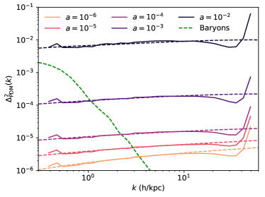
Figure 2: The PDM power spectrum as a function of scale factor, for $f_{\rm PBH}=0$. Solid curves show the results from our simulation whereas dashed curves correspond to linear-theory results from CLASS  Blas et al. (2011). Our simulations reproduce very well the growth of linear matter perturbations. The green dashed curve is the baryonic power spectrum at $a=10^{-2}$, and illustrates that baryons remain mostly unclustered on all scales of interest, at least in the linear regime.

We have also investigated the effects of the logarithmic time step limiter $ra_{\rm max}\geq da/(a+da)$, which prevents large jumps in redshift at early times, and the uniform offset applied each time step to avoid force artifacts when particles are outside the pp-force range due to the cubical rather than spherical particle search. We have increased the accuracy of both setting $ra_{\rm max}=0.005$ and allowing the offset to jump by up to 16 fine cells.

Lastly, we have tested the effects of gravitational softening in simulations containing a single PBH. The default softening is that of a hollow sphere of radius $1/10$ of a fine grid cell. Ideally, for the PBH there would be no softening as they truly are discrete objects. At great computational expense million particle $N$-body simulations with accurate binary orbital evolutions have been performed for globular clusters (Wang et al., 2015, 2016). However, it is unclear whether this can be done in a cosmological context as binary orbits remain fixed whereas the Universe expands. We therefore opt to soften the forces in our simulation. Since strong force effects tend to evaporate halos by ejecting PBH, we expect our results to be an upper bound on PBH-PDM clustering although we caution that the softening length can have different effects in simulations with multiple species compared to traditional PDM-only ones. For instance, artificial scattering of PDM particles can be enhanced due to the large PBH mass creating an unwanted numerical heating effect (Dehnen, 2001) or artificial collisionality can occur and inhibit even linear evolution (Angulo et al., 2013). We have explored the effects of various softening lengths in Appendix B and have found the default softening length to provide acceptable results in acceptable time.

We note a few potential issues with our evolution. The first one is non-spherical halo formation which occurs even if we turn off the adiabatic and isocurvature perturbations, i.e. even if we start PDM particles exactly on the grid. This can be seen in the top left panel of Fig. 1 and in the zoom-in showing the PDM particles in Fig. 3. This is likely due to the radial orbit instability which afflicts $N$-body systems even with very carefully set spherically symmetric initial conditions (e.g. (Vogelsberger et al., 2011), who also show that power law profiles still form despite the asphericity). We do not expect this effect to significantly affect any of our results. A second issue is the fact that box-sized modes begin to go nonlinear at $z=99$ for $f_{\rm PBH}\gtrsim 10^{-1}$ which could cause issues with power transfer from large to small scales (Bagla and Padmanabhan, 1997). Lastly, for simulations with $f_{\rm PBH}\ll 1$, the assumed periodicity of the simulation becomes artificial as we are not well sampling Poisson fluctuations on scales larger than the box size. This will introduce sample variance into our results that could affect quantities such as the halo mass function and perhaps PBH velocities when $f_{\rm PBH}\ll 1$, but should not affect halo profiles.

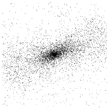
Figure 3: Zoom-in showing the PDM particles around the single PBH in our $f_{\rm PBH}=10^{-5}$ simulation (including adiabatic perturbations). Particles shown are in $(1/64)^{3}$ of the simulation box around the PBH. The PDM distribution is clearly aspherical in the outskirts, likely due to the radial orbit instability.

III.4 Halofinder

To understand gravitational clustering, we require estimates of how much PDM and PBH are bound in nonlinear halos. CUBEP³M has a run-time spherical overdensity halo finder. It first finds peaks in the PDM density field and then searches radially until the mean overdensity within $r$, $\Delta=\rho_{\rm PDM}(<r)/\bar{\rho}_{\rm PDM}$, drops to $\Delta_{\rm vir}\simeq 18\pi^{2}$. This defines the virial radius $r_{\rm HL}$. Note that the value of $\Delta_{\rm vir}$ has not been corrected for the presence of radiation, which is percent level at $z=99$. It also does not consider the PBH particles since only the PDM particles will have a smooth density field. Particles are not allowed to be in more than one halo, and halos are required to have at least $100$ PDM particles to be included in the catalogue. The halofinder is parallelized with the same volume decomposition as the main code, and therefore processes can find halos located outside their local volume. We do not include any such halos in order to avoid duplicates. We use the resulting halo virial masses as our estimate of the PDM accretion. Lastly, we note that at higher $f_{\rm PBH}$ the halofinder begins to find a small fraction of halos without PBH and that there are also many PBH that are not considered part of halos. This is certainly artificial, since even a perfectly isolated PBH should be called a halo. In the future, designing a dedicated $\Lambda$PBH halofinder could be warranted.

IV Results

IV.1 Matter power spectrum

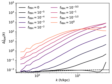
Figure 4: The PDM power spectrum as a function of $f_{\rm PBH}$ at $a=10^{-2}$. The presence of PBH causes significant nonlinear growth not found in standard $\Lambda$CDM.

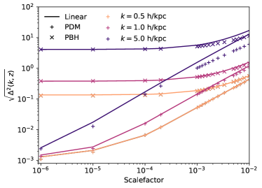
Figure 5: Growth of the PDM and PBH perturbation as a function of scale factor, for $f_{{\rm PBH}}=0.1$, and for several wavenumbers $k$. Linear theory matches the numerical result well, as long as $\Delta^{2}_{\rm PBH}\lesssim 1$.

We start by computing the PDM power spectrum which we show in Fig. 4. The black lines (solid is simulation, dashed is CLASS) show linear evolution of the PDM when there are no PBH ($f_{\rm PBH}=0$). The other curves show the resulting power spectra at $z=99$ as a function of $f_{\rm PBH}$. Increasing $f_{\rm PBH}$ disrupts the linear evolution at larger and larger scales, and completely dominates on all scales of the box for $f_{\rm PBH}\gtrsim 10^{-2}$. Interestingly, the PDM power spectrum turns over at large $k$ for high $f_{\rm PBH}$. This is likely due to the fact that halo profiles are very cuspy around isolated PBHs but significantly less so for halos containing multiple PBHs. The latter are more common as $f_{\rm PBH}$ is increased.

We next investigate the evolution of individual modes. We show the growth of density perturbations for several wavenumbers from the $f_{\rm PBH}=0.1$ simulation in Fig. 5 for both PDM and PBH. We compare this result to the linear evolution of PBH and PDM perturbations, derived in Section III.2.1. Note that linear theory only applies on scales where both $\delta_{\rm PDM}$ and $\delta_{\rm PBH}$ are small. In particular, it only applies for scales larger than the mean PBH separation. Using Eqs. (15)- (16) with $T_{\rm iso}(a)=D_{+}(a/a_{\rm eq})$ given by Eq. (23), and the fact that primordial adiabatic and isocurvature perturbations are uncorrelated, we find the following power spectra:

$$\Delta^{2}_{{\rm PDM}}(a) =\Delta_{\rm ad}^{2}(a)+f_{\rm PBH}^{2}\left(D_{+}(a)-1\right)^{2}(\Delta_{{\rm PBH}}^{0})^{2}~{}~{}~{}$$ (40)

$$\Delta^{2}_{\rm PBH}(a) =\Delta_{\rm ad}^{2}(a)$$

$$+\left[1+f_{\rm PBH}(D_{+}(a)-1)\right]^{2}(\Delta_{\rm PBH}^{0})^{2},$$ (41)

where $\Delta_{\rm ad}^{2}(a)$ is the power spectrum of the pure adiabatic mode at scale factor $a$, $(\Delta_{\rm PBH}^{0})^{2}$ is the primordial PBH (Poisson) power spectrum and we approximated $\delta_{\rm iso}^{0}\approx\delta_{\rm PBH}^{0}$.

We compare these results with those of our simulations in Fig. 5. We see that they agree quite well for linear modes, but increasingly differ as nonlinear evolution occurs, as can be expected. Interestingly, non-linear growth is slower than linear theory predicts.

IV.2 Halo properties

We begin by quantifying how much PDM and PBH are found within halos. We expect this to depend sensitively on $f_{\rm PBH}$. For small $f_{\rm PBH}$, PBHs will mostly be isolated from one another, and so halos can only increase mass by accumulating more and more PDM. On the other hand, for higher $f_{\rm PBH}$, the PBH themselves can become bound to one another, yielding potentially much larger halos with very different internal structures.

IV.2.1 PDM clustering in halos

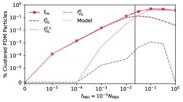
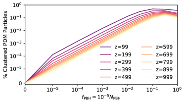
Figure 6: Top. Fraction of PDM contained within halos at $z=99$. The solid purple line shows the fraction of PDM in all halos. The dashed and dotted curves indicate the amount which is in halos with only one PBH and those with multiple PBHs, respectively. The grey vertical line is a prediction for their intersection. The dashed grey curve is the fraction of halos found without PBH. The orange curve shows a simple interpolating model. Bottom. The same fraction shown at a variety of redshifts.

We begin by computing the fraction of PDM particles that are clustered as a function of $f_{{\rm PBH}}$ which is given by $f_{\rm HL}=N_{{\rm PDM}\in{\rm HL}}/N_{\rm PDM}$ where $N_{{\rm PDM}\in{\rm HL}}$ is the number of PDM particles in halos. We show the results at $a=10^{-2}$ in the top panel of Fig. 6, alongside the fraction of PDM in halos without PBH ($f_{\rm HL}^{0}$). At $f_{\rm PBH}=0$ we find no halo as expected. We furthermore break $f_{\rm HL}$ based on whether it comes from a halo with one ($f_{\rm HL}^{1}$) or multiple ($f_{\rm HL}^{2+}$) PBH. There is a clear transition between isolated PBH ($f_{\rm HL}^{1}$) and clustered PBH ($f_{\rm HL}^{2+}$) that occurs between $10^{-2}<f_{\rm PBH}<10^{-1}$. To quantify this transition, we require knowledge of how PBH are distributed amongst halos of varying sizes, i.e. the halo mass function. A theoretical prediction, calculated in the next section, is shown as the grey vertical line, and agrees reasonably well with the numerical results.

This figure can be understood straightforwardly by considering limiting cases. For $f_{\rm PBH}\ll 1$, we expect halos to be well separated on average and accrete identically, so $f_{\rm HL}=c_{0}f_{\rm PBH}$. For $f_{\rm PBH}\sim 1$, we expect the majority of the PDM to be nonlinear, however only some fraction will be within halo virial radii and so $f_{\rm HL}=c_{1}$ when $\alpha\gg 1$. We show a simple interpolation between these limits:

$$f_{\rm HL}\simeq{\rm min}\left[c_{0}f_{\rm PBH},c_{1}\right]$$ (42)

where $c_{0}$ is the ratio of PDM halo fraction to PBH fraction for $f_{\rm PBH}=10^{-5}$ and $c_{1}$ is the ratio for $f_{\rm PBH}=10^{0}$. In the bottom panel of Fig. 6 we show the evolution of $f_{\rm HL}$ as a function of redshift. We tabulate the values of $c_{0}$ and $c_{1}$ in Table. 1. The coefficient $c_{0}$ scales approximately linearly with scale factor, as expected from the fact that the mass of PDM bound to a PBH is proportional to $(1-f_{\rm PBH})M_{\rm PBH}(a/a_{\rm eq})$ (see Mack et al. (2007) and Section III.2.2).

$z$	$c_{0}$	$c_{1}$
$999$	0.79	0.10
$299$	4.3	0.19
$99$	13	0.38

Table 1: Coefficients to compute the fraction of PDM particles in halos: $f_{\rm HL}={\rm min}[c_{0}f_{\rm PBH},c_{1}]$ as a function of redshift.

Understanding $f_{\rm HL}$ gives a straightforward way to estimate the halo mass as a function of the number of PBH it contains. Let $N_{{\rm PBH}/{\rm HL}}$ and $N_{{\rm PDM}/{\rm HL}}$ be the number of PBH and PDM particles in a halo. By definition, its mass is given by:

$$M_{\rm HL} =N_{{\rm PBH}/{\rm HL}}m_{\rm PBH}+N_{{\rm PDM}/{\rm HL}}m_{\rm PDM}$$ (43)

$$=N_{{\rm PBH}/{\rm HL}}m_{\rm PBH}\left[1+\frac{N_{{\rm PDM}/{\rm HL}}}{N_{{\rm PBH}/{\rm HL}}}\frac{m_{\rm PDM}}{m_{\rm PBH}}\right].$$ (44)

If we now assume that $N_{{\rm PDM}/{\rm HL}}$ is directly proportional to $N_{{\rm PBH}/{\rm HL}}$ and that all PBH are in halos, we can obtain $N_{{\rm PDM}/{\rm HL}}=N_{{\rm PBH}/{\rm HL}}\frac{N_{\rm PDM}}{N_{\rm PBH}}\frac{f_{\rm HL}}{1-f_{\rm PBH}}$ (this is equivalent to assuming $N_{{\rm PDM}/{\rm HL}}=N_{{\rm PDM}\in{\rm HL}}/N_{\rm HL}$ and $N_{{\rm PBH}/{\rm HL}}=N_{\rm PBH}/N_{\rm HL}$). Using this relation the halo mass becomes:

$$M_{\rm HL} \simeq N_{{\rm PBH}/{\rm HL}}m_{\rm PBH}\left[1+f_{\rm HL}\frac{1-f_{\rm PBH}}{f_{\rm PBH}}\right].$$ (45)

We show this result in Fig. 7 and find the approximation is accurate to a factor of a few.

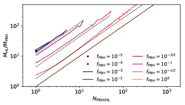
Figure 7: Halo mass as a function of the number of PBH contained within the halo virial radius. A simple interpolating model is also shown as dotted lines.

IV.2.2 Halo Mass Function

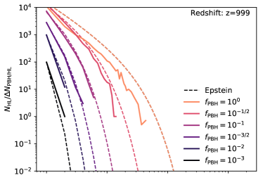
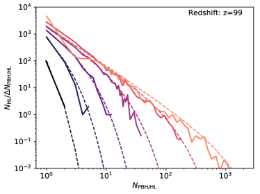
Figure 8: The abundance of halos containing a given number of PBH, which we call the halo mass function. Solid lines are determined from $N$-body simulations. Dashed lines are theoretical predictions assuming Poisson statistics.

In order to determine when halo growth occurs via quasi-spherical accretion or mergers, we need to be able to determine how many PBH are isolated as a function of $f_{\rm PBH}$. To do this, we compute the number of halos containing a given number of PBH, $N_{\rm HL}(N)$, where, for notational simplicity, we use $N=N_{{\rm PBH}/{\rm HL}}$ in this discussion. As we have shown in Fig. 7, the halo mass is nearly linearly related to the number of PBH it contains. We will therefore refer to $N_{\rm HL}(N)$ as the halo mass function. For initially Poisson-distributed particles, Epstein (1983) computed the exact distribution arising from an initial density $\delta_{\rm PBH}^{I}>\delta_{*}$ as:

$$N_{\rm HL}(N) =\frac{N_{\rm PBH}}{N}\frac{\delta_{*}}{1+\delta_{*}}\left(\frac{N}{1+\delta_{*}}\right)^{N-1}\frac{\exp\left[-\frac{N}{1+\delta_{*}}\right]}{(N-1)!}$$

$$=\delta_{*}\frac{N_{{\rm PBH}}}{N}\frac{(N/e)^{N}}{N!}\textrm{e}^{-N/N_{*}}$$

$$N_{*} \equiv\left(\log(1+\delta_{*})-\frac{\delta_{*}}{1+\delta_{*}}\right)^{-1},$$ (46)

where $N_{\rm PBH}=10^{5}f_{\rm PBH}$ is the total number of PBHs.

For $N\gg 1$, we may use Stirling’s approximation for the factorial and obtain

$$N_{\rm HL}(N)\approx \frac{\delta_{*}~{}N_{\rm PBH}}{\sqrt{2\pi}N^{3/2}}\textrm{e}^{-N/N_{*}}.$$ (47)

The fractional error of this approximation is $0.08/N$, independent of $\delta_{*}$; this approximation is therefore accurate to better than 10% even for $N\sim 1$.

When $\delta_{*}\ll 1$, we may Taylor-expand $N_{*}^{-1}\approx\delta_{*}^{2}/2+\mathcal{O}(\delta_{*}^{3})$. Provided $N\ll\delta_{*}^{-3}\sim N_{*}^{3/2}$, we may neglect terms of order $N\delta_{*}^{3}$ in the exponent and recover (Epstein, 1983) the Press-Schechter function (Press and Schechter, 1974)

$$N_{\rm HL}(N)\approx\frac{\delta_{*}~{}N_{\rm PBH}}{\sqrt{2\pi}N^{3/2}}\exp\left[-\frac{\delta_{*}^{2}}{2}N\right].$$ (48)

In practice, this approximation always breaks down for sufficiently large $N$ and we only use Eqs. (IV.2.2) or (47).

For a given scale factor $a$, the minimum initial PBH overdensity $\delta_{*}$ is determined as follows. We require that the initial total CDM overdensity $\delta_{c}^{I}=f_{{\rm PBH}}\delta_{*}$ has collapsed into a halo by scale factor $a$ (this assumes negligible fluctuations in the PDM component). This is equivalent to requiring that the linearly-extrapolated CDM overdensity $\delta_{\rm lin}(a)=D_{+}(a)\delta_{c}^{I}$ has reached a critical value $\delta_{\rm cr}(a)$, where $D_{+}$ is computed in Section IV.1. This implies

$$\delta_{*}(a)=\frac{\delta_{\rm cr}(a)}{D_{+}(a)f_{{\rm PBH}}}.$$ (49)

When collapse occurs well inside matter domination, and when baryons cluster like dark matter, the critical density is $\delta_{\rm cr}=1.69$. However, it can differ significantly from this value as collapse occurs closer to matter-radiation equality, and on scales where baryons remain unclustered. We explicitly compute $\delta_{\rm cr}(a_{\rm coll})$ in Appendix A. We find, for instance, that $\delta_{\rm cr}\approx 2.07$ at $z=999$, and even at $z=99$, $\delta_{\rm cr}\approx 1.71$. The minimum initial PBH overdensity is therefore $\delta_{*}\approx 0.43/f_{\rm PBH}$ and $0.052/f_{\rm PBH}$ at $z=999$ and 99, respectively. We find that the Epstein mass function (IV.2.2), with $\delta_{i}$ given by Eq. (49), give a good match to our halo mass function at $z=99$, see lower panel of Fig. 8. The Epstein function also matches our halo mass function reasonably well at $z=999$ for $f_{\rm PBH}\lesssim 10^{-1/2}$, see upper panel of Fig. 8. The poorer match at $f_{\rm PBH}=1$ could be due to our halo finder, which is exclusively based on PDM particles and misses some PBH.

Given the number function, Eq. (IV.2.2), we can now compute the value of $f_{\rm PBH}$ for which halo formation transitions from the seed to the Poisson mechanism. Specifically, this is when half the PBH are in halos with 1 PBH, or

$$\frac{N_{{\rm HL}}(1)}{N_{\rm PBH}}=\frac{\delta_{*}}{1+\delta_{*}}\exp\left[\frac{-1}{1+\delta_{*}}\right]=\frac{1}{2}.$$ (50)

This is satisfied for $\delta_{*}=2.175$ so $f_{\rm PBH}\simeq 0.02(1+z)/100$. This prediction is shown in Fig. 6 as the vertical grey line and matches the numerical result quite well.

IV.2.3 Halo Profiles

We now consider the PDM density profiles that form around the halos in the simulation. We start by considering the single isolated PBH in the $f_{\rm PBH}=10^{-5}$ simulation and show its profile as a function of redshift in Fig. 9. At early times ($a=10^{-3}$), we find a profile with power law slope of $-2.28\pm 0.08$ which is consistent with both the theoretical prediction ($-2.25$) and other numerical simulations Adamek et al. (2019). At later times the profile becomes steeper, with a slope of $-2.55\pm 0.04$ at $a=10^{-2}$.

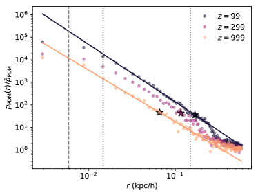
Figure 9: Spherically averaged PDM density profiles around the single black hole in the $f_{\rm PBH}=10^{-5}$ simulation as a function of comoving radius, and for several redshift. We find that the profile features a power law at all times, which steepens as time progresses. Best-fit power laws at $a=10^{-3}$ and $a=10^{-2}$ are shown as solid lines. The dashed grey curve indicates the force softening length whereas the dotted grey curves indicate the radii included in the power law fit. The stars indicate the halo virial radii.

Next, we investigate how the PDM profiles vary with $f_{\rm PBH}$ at $a=10^{-2}$. We identify halos containing only a single PBH and compute the average PDM density profile of all such halos. We show the result in Fig. 10, with error bands showing the standard deviation. We find that a power law profile is retained, regardless of $f_{\rm PBH}$ but that the slope becomes steeper with increasing $f_{\rm PBH}$, up to a value of $-3.24\pm 0.04$ for $f_{\rm PBH}=1$. We note that we slightly reduced the fit range since the halo radii are significantly smaller at higher $f_{\rm PBH}{}$.

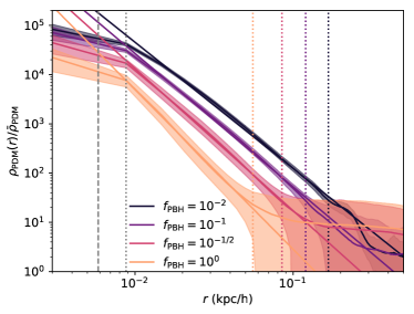
Figure 10: Average PDM density profiles around halos containing a single PBH at $a=10^{-2}$, as a function of $f_{\rm PBH}$, with error bands showing the standard deviation. We find that PDM halos around isolated PBH have power law profiles, whose slope steepens with increasing $f_{\rm PBH}$. The dashed line shows the softening length, whereas dotted lines indicate the fit region, with largest value being the halo virial radius.

Finally, we consider halos containing more than one PBH. As an example, we show in Fig. 11 the mean density profile of halos containing between 13 and 17 PBH. We find the profile to be significantly shallower. While it is suggestive that the profiles are more cored than power law, we caution that softening is likely playing a role and higher resolution simulations are necessary to determine if the profile turns over.

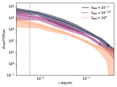
Figure 11: PDM density profiles around halos containing between 13 and 17 PBH at $a=10^{-2}$. The profiles are significantly shallower than the power laws seen in Fig. 10.

IV.3 Nonlinear PBH Velocities

We now turn our attention to the PBH velocity distribution. Determining this quantity is relevant for CMB constraints as it will affect the accretion rate of gas onto PBH in the early Universe Ricotti et al. (2008); Ali-Haïmoud and Kamionkowski (2017); Poulin et al. (2017). There are two contributions to the variance of the PBH velocity distribution: a large-scale piece $\langle v_{\rm L}^{2}\rangle$, due to linear perturbations on scales $k_{\rm box}\lesssim k\lesssim k_{\rm NL}$, and a small-scale piece $\langle v_{\rm NL}^{2}\rangle$, arising from virial motions inside halos.

The large-scale contribution can be estimated from the linearized continuity equation for PBHs:

$$\vec{v}_{\rm L} =i\frac{\hat{k}}{k}\dot{\delta}_{{\rm PBH}}=i\hat{k}\frac{aH}{k}\frac{d\ln\delta_{\rm PBH}}{d\ln a}\delta_{\rm PBH}.$$ (51)

Since we restrict ourselves to linear scales, the variance of PBH density fluctuations per $\ln k$ scales as $k^{3}$, like their initial Poisson distribution. As a consequence the variance of $\vec{v}_{\rm L}$ per $\ln k$ scales as $k$, and is dominated by the smallest relevant scale, i.e. the non-linear scale $k_{\rm NL}$. By definition, this is the scale at which $\delta_{\rm PBH}\sim 1$. Hence we find

$$\langle v_{\rm L}^{2}\rangle^{1/2}\sim\frac{aH}{k_{\rm NL}}\frac{d\ln\delta_{\rm PBH}}{d\ln a}.$$ (52)

To estimate $k_{\rm NL}$ and $d\ln\delta_{\rm PBH}/d\ln a$, we use Eq. (25), in the limit where PBHs dominate the initial density perturbations. We moreover simplify matters by taking the limit where baryons cluster like CDM, so that:

$$\delta_{\rm PBH}\approx\left(1+\frac{3}{2}\frac{a}{a_{\rm eq}}f_{\rm PBH}\right)\delta_{\rm PBH}^{I}.$$ (53)

This implies

$$\frac{d\ln\delta_{{\rm PBH}}}{d\ln a} \approx\frac{\frac{3}{2}\frac{a}{a_{\rm eq}}f_{\rm PBH}}{1+\frac{3}{2}\frac{a}{a_{\rm eq}}f_{\rm PBH}},$$ (54)

$$k_{\rm NL} \approx\left(\frac{2\pi^{2}\overline{n}_{{\rm PBH}}}{(1+\frac{3}{2}\frac{a}{a_{\rm eq}}f_{\rm PBH})^{2}}\right)^{1/3},$$ (55)

where $\overline{n}_{\rm PBH}$ is the comoving number density of PBHs, which sets the amplitude of initial Poisson perturbations. Numerically, we obtain

$$v_{\rm L}\sim 1\ \textrm{km/s}\ \frac{f_{\rm PBH}^{2/3}(a/a_{\rm eq})^{1/2}}{\left(1+\frac{3}{2}\frac{a}{a_{\rm eq}}f_{\rm PBH}\right)^{1/3}}.$$ (56)

For instance, at $z=300$, and for $f_{\rm PBH}=0.1$, this estimate gives $v_{\rm L}\sim 0.5$ km/s. We find that isolated PBHs (which do not belong to halos with multiple PBHs) indeed have a characteristic velocity of that order, see Fig. 12.

We now estimate the non-linear velocity, based on the halo model developed in the preceding section. The behaviour of a PBH in a halo depends significantly on $N_{{\rm PBH}/{\rm HL}}$. An isolated PBH will simply sit in the halo center of mass (having seeded its formation in the first place), and therefore moves with the halo motion. On the other hand, if the halo hosts a multitude of virialized PBH, their motions will include a virial velocity:

$$V_{\rm HL}^{2}\sim\frac{GM_{\rm HL}}{aR_{\rm HL}}$$ (57)

where we use Eq. 45 for $M_{\rm HL}$ and $R_{\rm HL}$ is the comoving halo radius. We can estimate $R_{\rm HL}$ via:

$$\Delta_{\rm vir}\bar{\rho}_{c}=\frac{M_{\rm HL}}{\frac{4}{3}\pi(R_{\rm HL})^{3}}$$ (58)

Note that these virial velocities do not depend particularly sensitively on the definition of the halo (i.e. the value of $\Delta_{\rm vir}$). We approximate the probability distribution of a ${\rm PBH}$ in a halo with $N_{{\rm PBH}/{\rm HL}}$ as a 3-dimensional Gaussian with variance $\sigma_{v}^{2}$:

$$\frac{dP}{dv}(N_{{\rm PBH}/{\rm HL}})=\sqrt{\frac{2}{\pi}}\frac{v^{2}}{\sigma_{v}^{3}}\exp\left[-\frac{v^{2}}{2\sigma_{v}^{2}}\right]$$ (59)

where $3\sigma_{v}^{2}=V_{\rm HL}^{2}+v_{\rm L}^{2}$ depends on $N_{{\rm PBH}/{\rm HL}}$. The differential distribution of PBH velocities is obtained by summing over all halos:

$$\frac{dN_{\rm PBH}}{dv}=\sum\limits_{N=2}^{\infty}NN_{\rm HL}(N)\frac{dP}{dv}(N).$$ (60)

We compute this distribution using Eq. (45) for $M_{\rm HL}$ and Eq. (IV.2.2) for the mass distribution. Our results are shown in Fig. 12 where we see that the halo model prediction does a reasonable job in modeling the true distribution. Since Eq. 57 is only accurate to factors of order unity, this model only provides an order of magnitude estimate even if the agreement for $f_{\rm PBH}=10^{-1}$ appears rather good.

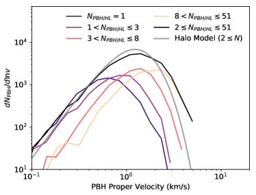
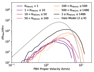
Figure 12: The number of PBH per unit velocity as a function of PBH velocities at $z=99$ for $f_{\rm PBH}=10^{-1}$ (top) and $10^{0}$ (bottom). The grey curve shows a prediction via the halo model and should be compared to the black curve. The warm coloured lines show components originating from HL with different numbers of PBH. Note that we only consider PBH found by the halofinder in this figure.

We show the velocity dispersion $\sqrt{\langle v^{2}\rangle-\langle\vec{v}\rangle^{2}}$ as a function of redshift in Fig. 13. We find that it increases by an order of magnitude between $f_{\rm PBH}=10^{-3}$ and $f_{\rm PBH}=10^{0}$. We compare this velocity dispersion to the characteristic large-scale velocity of the gas relative to dark matter and the gas sound speed Tseliakhovich and Hirata (2010)

$$v_{\rm rel} \approx 30~{}{\rm km}/{\rm s}\frac{1+z}{1000},$$ (61)

$$c_{s} \approx 6~{}{\rm km}/{\rm s}\sqrt{\frac{1+z}{1000}}.$$ (62)

We see in Fig. 13 that the typical non-linear motions are smaller than the baryon sound speed for $z\gtrsim 300$, even for $f_{\rm PBH}\rightarrow 1$. This suggests that, even in patches of low relative velocity, baryons may not be efficiently captured in the first PBH + PDM halos until $z\lesssim 300$. In regions with typical relative velocities, baryons may not be efficiently accreted until $z\lesssim 100$. Thus, even though small-scale dark matter structures form much earlier than in standard PDM cosmology, it is unclear whether and when they would acquire a significant baryon content. It would be interesting to address this question with dedicated hydrodynamical simulations.

Non-linear velocities could in principle affect CMB limits to accreting PBHs Ricotti et al. (2008); Ali-Haïmoud and Kamionkowski (2017); Poulin et al. (2017). At equal gas density, larger velocities would decrease the accretion rate. However, once the gas gets bound to halos, it may get significantly denser than the cosmological average. Within the most conservative “collisional ionization” limit of Ali-Haïmoud and Kamionkowski (2017), we have checked that completely switching off black hole accretion at $z<300$ has a negligible impact on CMB bounds. Conversely, increasing the PBH luminosity by a factor of 10 at $z<300$ tightens CMB upper limits by no more than $\sim 10\%$, and only at the highest mass end. It is therefore unlikely that CMB limits are significantly affected by non-linear velocities, though a definitive conclusion would require more detailed modeling of both the baryon distribution, as well as the accretion process. Note that Ref. Hütsi et al. (2019) recently reached the same conclusion, using analytic estimates of the PBH velocity distribution, although they did not explicitly check the effect on CMB limits as we do here.

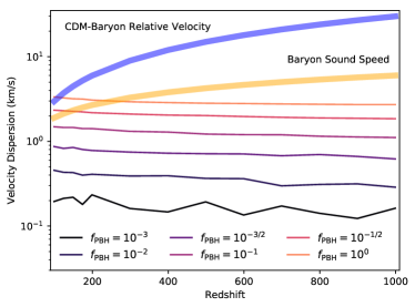
Figure 13: The PBH velocity dispersion as a function of $f_{\rm PBH}$ and redshift. PBH clustering increases the velocities of PBH, but not to speeds comparable to the relative velocity effect.

IV.4 Approximate self-similarity

While our results have specifically focused on the case where $M_{\rm PBH}=20M_{\odot}h^{-1}$, we note that our simulations are approximately self-similar, hence our results can be easily transposed to different PBH masses. First of all, Hamilton’s equations are invariant under the following rescaling of positions, velocities and masses:

$$x\rightarrow\lambda x$$

$$v\rightarrow\lambda v$$

$$M\rightarrow\lambda^{3}M$$ (63)

Secondly, the initial random distribution of PBHs is exactly scale-invariant. Finally, the adiabatic initial perturbations are not strictly scale invariant, but are nearly so on the scales of interest.

Our simulation setup explicitly respects the self-similarity of the underlying equations. Before applying displacement fields, the PDM particles are set on a cubical lattice, a structure which is clearly independent of scale. Similarly, the distribution of PBH particles is completely random, and therefore also cannot depend on box size. The simulation box size only enters explicitly when setting the adiabatic initial conditions. Subsequent gravitational evolution only depends on the particles’ numerical mass (Eq. 39) which is again independent of any physical scale. Our simulation setup therefore explicitly preserves the approximate self-similarity given by Eq. (63).

Of course, approximate self-similarity does not extend to arbitrary scales. In particular, for $M_{\rm PBH}\gtrsim 10^{4}M_{\odot}$, the box size exceeds the horizon scale at the starting redshift. This is unlikely to be a severe issue, however, since there is not much gravitational evolution until matter-radiation equality, at which point the horizon size exceeds the box size as long as $M_{\rm PBH}\lesssim 10^{11}M_{\odot}$. More importantly, while the simulation scales satisfy $k\propto M_{\rm PBH}^{-1/3}$, the scale $k_{*}$ of the enhancement in the primordial power spectrum required to form PBHs has a steeper scaling $k_{*}\propto M_{\rm PBH}^{-1/2}$ Sasaki et al. (2018). Given our fiducial box and grid size, the grid scale would exceed $2\pi/k_{*}$ for $M_{\rm PBH}\gtrsim 10^{7}M_{\odot}$, and we could no longer extrapolate the primordial large-scale power spectrum all the way down to the grid scale. On the other hand, there does not appear to be an obvious limitation to rescaling our simulations to smaller PBH masses.

V Discussion and Conclusion

We have studied how structure forms in $\Lambda$PBH cosmologies containing a mixture of primordial black holes (PBH) and standard particle dark matter (PDM). Our results depend sensitively on what fraction of the CDM is in the form of PBH. For $f_{\rm PBH}\lesssim z\times 10^{-4}$, the PBH are generally isolated from one another and accrete PDM to form halos. For $f_{\rm PBH}\gtrsim z\times 10^{-4}$, there is significantly more clustering of PBH to form much larger halos. We find that halo masses are nearly linearly proportional to the number of PBH they contain and that the halo mass function is well described via Poisson statistics. Isolated halos containing only a single black hole tend to form steep power law PDM distributions, regardless of $f_{\rm PBH}$. On the other hand, such steep profiles do not occur when the halos contain many virialized PBH. We quantified the nonlinear velocities of PBH and find them strongly subdominant to the relative velocity between gas and CDM for $z\gtrsim 300$. We showed that they should not significantly affect CMB constraints to accreting PBH (Ali-Haïmoud and Kamionkowski, 2017). While we only ran simulations with $M_{\rm PBH}=20~{}h^{-1}M_{\odot}$, we argued that our simulations are approximately self-similar, and can be simply rescaled to arbitrary PBH mass, up to a maximum mass of $\sim 10^{7}M_{\odot}$.

Current limitations on our simulations are largely computational. For instance, it would be beneficial for the $f_{\rm PBH}=1$ simulation to evolve a larger volume so that the adiabatic perturbations are resolved and box-scale modes do not become nonlinear. Increasing the number of PDM particles would also lead to better resolved halo inner structures. It is also challenging to extrapolate our results to the present day which impacts our ability to determine if these PBH minihalos survive and may be present in the galactic halo. This is of crucial importance for some constraints due to PDM annihilation (Lacki and Beacom, 2010) or astrometry Van Tilburg et al. (2018).

With the development of the numerical simulation code, computations that are challenging analytically become more tractable. We are particularly interested in studying the Poisson clustering of PBH, which should lead to the formation of many binaries deep in the radiation era. If such binaries survive until the present, then LIGO will have already put significant constraints on $f_{\rm PBH}$ (Ali-Haïmoud et al., 2017). However, these constraints rely on many approximations that require numerical verification. Ref. (Kavanagh et al., 2018) studied the interaction of pairs of PBH initially clothed by PDM. They find that as the PBH orbit, they lose their PDM halos and dynamical friction effects tend to circularize and shrink the orbit. Overall, however, the effects are modest provided the initial eccentricity is large. A different mechanism for disrupting the binaries is nontrivial tidal forces. Ref. (Raidal et al., 2018) simulated binary PBH surrounded by other PBH (but not PDM). They find that binaries are frequently disrupted for $f_{\rm PBH}\gtrsim 10^{-1}$. While our numerical setup does not have high enough spatial resolution to resolve individual binary orbits, they should allow us to understand the tidal field the binary is immersed in. We expect to obtain complementary information to Refs. (Kavanagh et al., 2018; Raidal et al., 2018) since our simulations contain both PDM and PBH, can go an order of magnitude lower in redshift, and probe halos with many more PBH.

Another interesting computation is the effect of $\Lambda$PBH on cosmic dawn. In the standard picture, in the absence of PBHs, first stars are expected to typically form when CDM halos reach a mass of $10^{6}M_{\odot}$ (Visbal et al., 2012). Given that halos tend to form much earlier in $\Lambda$PBH (even with a subdominant fraction of DM in PBHs), it is possible that the first lights in the Universe turn on earlier. Such a modification to early star formation by PBH has been studied analytically in Ref. (Kashlinsky, 2016) who found it could explain the remnant cosmic infrared background fluctuations that cannot be explained via observed galaxies. We expect that this analysis can be improved by extracting the virial temperature, $T\propto M/R$, as a function of halo mass since the formation of first stars is largely sensitive to the gas temperature. It may become necessary to simulate the baryons as well, although this would require modelling their CMB interactions, and later on radiative processes from star formation.

Another area to explore is how much PBH clustering is affected when the adiabatic power spectrum is not the standard $\Lambda$CDM one but rather is enhanced on certain scales. Such a change in the adiabatic power spectrum is also likely to affect the PBH binaries (Garriga and Triantafyllou, 2019) and cosmic dawn (Hirano et al., 2015) as well. We intend to tackle these interesting questions in future publications.

VI Acknowledgements

We acknowledge valuable technical support and discussions with Hao-ran Yu, Ue-Li Pen and JD Emberson. We thank Daniel Grin, Neal Dalal, Ravi Sheth and Joe Silk for useful conversations. This work was made possible in part through the NYU IT High Performance Computing resources, services, and staff expertise. We acknowledge the use of NumPy (van der Walt et al., 2011), SciPy Jones et al. (2001–), Matplotlib (Hunter, 2007) and NASA’s Astrophysics Data System Bibliographic Services. This research is supported by the National Science Foundation under Grant No. 1820861.

Appendix A Spherical top-hat collapse in matter and radiation era

The famous value of the linearly-extrapolated density at collapse, $\delta_{\rm cr}=1.686$, is only valid for collapse that occurs entirely in matter domination. This is an accurate approximation for halos collapsing around redshift 0 (or rather, around redshift of a few, before dark-energy domination). It needs not be accurate for halos collapsing at $z\gtrsim 100$, of interest here, for which radiation contributed a significant part of the energy density, at least in the initial phases of the evolution. Furthermore, prior to kinematic decoupling around $z\sim 10^{3}$, baryons are subject to strong Compton drag, which prevents their clustering on all scales. On scales smaller than the baryon Jeans scale, they remain unclustered even after decoupling from CMB photons. To account for these effects, we generalize the spherical top-hat collapse model Gunn and Gott (1972) to a halo of cold dark matter collapsing in a Universe comprised of matter and radiation (the latter assumed fully homogeneous), assuming only the cold dark matter clusters, and baryons remains homogeneous. This setup is similar in spirit to that of Refs. LoVerde (2014), who studied spherical top-hat collapse in the presence of free-streaming neutrinos. See also Ref. Naoz and Barkana (2007) for a similar study, with different setup (we assume baryons remain unclustered throughout the collapse, being interested in sub-Jeans scale perturbations). We restrict ourselves to deeply sub-horizon scales. We define $\gamma\equiv\Omega_{c}/\Omega_{m}$ to be the fraction of clustered matter.

While the density perturbations become non-linear, metric perturbations remain small, and we may assume a perturbed FLRW metric. We assume a uniform, top-hat dark matter overdensity $\delta(a)$, within a comoving radius $R(a)$. The constant CDM mass contained in this region is $M=\frac{4\pi}{3}\overline{\rho}_{c,0}(1+\delta)R^{3}=\frac{4\pi}{3}\overline{\rho}_{c,0}(1+\delta_{i})R_{i}^{3}$, where $\overline{\rho}_{c,0}=\gamma\rho_{m,0}$ is the background comoving CDM density, and $R_{i}$ and $\delta_{i}$ are the initial radius and overdensity, respectively. Combining the geodesic equation for $R(a)$ with the Poisson equation, and defining $\chi\equiv R/R_{i}$, we obtain the following differential equation for $\chi(s=a/a_{\rm eq})$:

$$2s(1+s)\chi^{\prime\prime}(s)+(2+3s)\chi^{\prime}(s)=\gamma\left(\chi-\frac{1+\delta_{i}}{\chi^{2}}\right).$$ (64)

This equation must be solved subject to initial conditions $\chi(0)=1,\chi^{\prime}(0)=-\frac{\gamma}{2}\delta_{i}$, the latter being the only well-behaved initial condition for the initial velocity. Given an initial overdensity $\delta_{i}$, we solve this equation up until the time $s_{\rm coll}$ at which $\chi$ vanishes.

The CDM overdensity is related to $\chi$ through $(1+\delta)=(1+\delta_{i})/\chi^{3}$. We define $\delta_{\rm lin}(s)$ to be the solution of the linearized fluid equation for the overdensity. Assuming an initially constant overdensity, we have $\delta_{\rm lin}(a)=D_{+}(a)\delta_{i}$, where $D_{+}$ is the linear growth rate computed in Section III.2.1. For a given $\delta_{i}$, we compute the linearly-extrapolated overdensity at the time of collapse $s_{\rm coll}$, $\delta_{\rm lin}(s_{\rm coll})=D_{+}(s_{\rm coll})\delta_{i}$. We show this critical density as a function of collapse scale factor in Fig. 14.

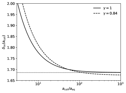
Figure 14: Linearly-extrapolated dark matter overdensity at collapse, as a function of collapse scale factor, assuming a homogeneous radiation background. The dotted line shows the standard value $\delta_{\rm cr}=1.686$, which holds when collapse occurs deep in the matter-domination era. The solid line shows the critical overdensity when all the matter clusters. The dashed line show the corresponding value when only a fraction $0.84$ of the matter clusters.

Appendix B Convergence Tests

In this Appendix we seek to check the dependence of our results on three different factors: (1) the force softening length, (2) the initial conditions, and (3) the number of PDM particles. To do this we setup simulations with $10^{4}$ PBH and $2\times 128^{3}$ PDM particles each with no initial perturbations (i.e. a pure Poissonian distribution of PBH and lattice distribution of PDM). We run four of these simulations with varying softening length $r_{\rm soft}=0.2,0.1,0.05$ and $0.025$ fine cells. These simulations can then be compared to the reference $f_{\rm PBH}=10^{-1}$ simulation in the main text. Note that since the particle number has changed, it is the $0.05$ softening length that is equivalent to the reference simulation. The results we expect to be most sensitive to softening are the profiles of halos with many PBH and the PBH virial velocities. We show the former in Fig. 15. While it is clear that softening plays a significant role on the inner parts of the halo, it appears that smaller softening lengths produce even flatter cores. Nonetheless, higher particle numbers are still needed to confirm. The PBH velocity dispersion as a function of redshift are shown in Fig. 16. We find that our choice of softening length actually yields the largest dispersion. We expect this to not change our conclusions as we had already argued that these velocities are small.

We have also considered and tested using different softening length for the PBH and the PDM, since ideally the PBH would be softened significantly less. This is not an issue for simulations with low number density where PBH never are nearby one another, but is an issue at higher number densities. For simulations where PBH are numerous enough to require softening in the PBH-PBH force, we find that the smallest softening length determines total runtime. There is therefore no benefit to not using the smallest softening length for all particles. This likely would not be true if different particles could have different timesteps, in which case it could be beneficial to set the PBH softening length lower. However, such a feature is currently not implemented in CUBEP³M.

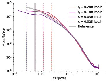
Figure 15: Convergence test of Fig. 11. The grey band shows the result presented in the main text, whereas the other curves arise from simulations with 1/8 the number of PDM particles, no initial conditions, and varying the softening length.

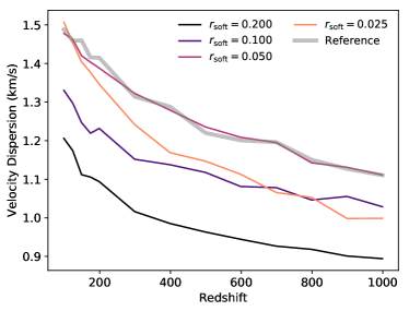
Figure 16: Convergence test of Fig. 13. Otherwise same description as Fig. 15.

References

- Jungman et al. (1996) G. Jungman, M. Kamionkowski, and K. Griest, Phys. Rep. 267, 195 (1996), eprint hep-ph/9506380.
- Bullock and Boylan-Kolchin (2017) J. S. Bullock and M. Boylan-Kolchin, ARA&A 55, 343 (2017), eprint 1707.04256.
- Dodelson and Widrow (1994) S. Dodelson and L. M. Widrow, Physical Review Letters 72, 17 (1994), eprint hep-ph/9303287.
- Hu et al. (2000) W. Hu, R. Barkana, and A. Gruzinov, Physical Review Letters 85, 1158 (2000), eprint astro-ph/0003365.
- Marsh (2016) D. J. E. Marsh, Phys. Rep. 643, 1 (2016), eprint 1510.07633.
- Zel’dovich and Novikov (1967) Y. B. Zel’dovich and I. D. Novikov, Soviet Ast. 10, 602 (1967).
- Hawking (1971) S. Hawking, MNRAS 152, 75 (1971).
- Carr and Hawking (1974) B. J. Carr and S. W. Hawking, MNRAS 168, 399 (1974).
- Carr et al. (2016) B. Carr, F. Kühnel, and M. Sandstad, Phys. Rev. D 94, 083504 (2016), eprint 1607.06077.
- García-Bellido (2017) J. García-Bellido, in Journal of Physics Conference Series (2017), vol. 840 of Journal of Physics Conference Series, p. 012032, eprint 1702.08275.
- Abbott et al. (2016a) B. P. Abbott, R. Abbott, T. D. Abbott, M. R. Abernathy, F. Acernese, K. Ackley, C. Adams, T. Adams, P. Addesso, R. X. Adhikari, et al., Physical Review Letters 116, 061102 (2016a), eprint 1602.03837.
- Abbott et al. (2016b) B. P. Abbott, R. Abbott, T. D. Abbott, M. R. Abernathy, F. Acernese, K. Ackley, C. Adams, T. Adams, P. Addesso, R. X. Adhikari, et al., Physical Review Letters 116, 241103 (2016b), eprint 1606.04855.
- Abbott et al. (2017a) B. P. Abbott, R. Abbott, T. D. Abbott, F. Acernese, K. Ackley, C. Adams, T. Adams, P. Addesso, R. X. Adhikari, V. B. Adya, et al., Physical Review Letters 118, 221101 (2017a), eprint 1706.01812.
- Abbott et al. (2017b) B. P. Abbott, R. Abbott, T. D. Abbott, F. Acernese, K. Ackley, C. Adams, T. Adams, P. Addesso, R. X. Adhikari, V. B. Adya, et al., ApJ 851, L35 (2017b), eprint 1711.05578.
- Abbott et al. (2017c) B. P. Abbott, R. Abbott, T. D. Abbott, F. Acernese, K. Ackley, C. Adams, T. Adams, P. Addesso, R. X. Adhikari, V. B. Adya, et al., Physical Review Letters 119, 141101 (2017c), eprint 1709.09660.
- Bird et al. (2016) S. Bird, I. Cholis, J. B. Muñoz, Y. Ali-Haïmoud, M. Kamionkowski, E. D. Kovetz, A. Raccanelli, and A. G. Riess, Physical Review Letters 116, 201301 (2016), eprint 1603.00464.
- Clesse and García-Bellido (2017) S. Clesse and J. García-Bellido, Physics of the Dark Universe 15, 142 (2017), eprint 1603.05234.
- Sasaki et al. (2016) M. Sasaki, T. Suyama, T. Tanaka, and S. Yokoyama, Physical Review Letters 117, 061101 (2016), eprint 1603.08338.
- Planck Collaboration et al. (2016) Planck Collaboration, P. A. R. Ade, N. Aghanim, M. Arnaud, M. Ashdown, J. Aumont, C. Baccigalupi, A. J. Banday, R. B. Barreiro, J. G. Bartlett, et al., A&A 594, A13 (2016), eprint 1502.01589.
- Jeong et al. (2014) D. Jeong, J. Pradler, J. Chluba, and M. Kamionkowski, Physical Review Letters 113, 061301 (2014), eprint 1403.3697.
- Nakama et al. (2014) T. Nakama, T. Suyama, and J. Yokoyama, Physical Review Letters 113, 061302 (2014), eprint 1403.5407.
- Ricotti and Gould (2009) M. Ricotti and A. Gould, ApJ 707, 979 (2009), eprint 0908.0735.
- Gosenca et al. (2017) M. Gosenca, J. Adamek, C. T. Byrnes, and S. Hotchkiss, Phys. Rev. D 96, 123519 (2017), eprint 1710.02055.
- Delos et al. (2018) M. S. Delos, A. L. Erickcek, A. P. Bailey, and M. A. Alvarez, Phys. Rev. D 97, 041303 (2018).
- Sten Delos et al. (2018) M. Sten Delos, A. L. Erickcek, A. P. Bailey, and M. A. Alvarez, arXiv e-prints arXiv:1806.07389 (2018), eprint 1806.07389.
- Hirano et al. (2015) S. Hirano, N. Zhu, N. Yoshida, D. Spergel, and H. W. Yorke, ApJ 814, 18 (2015), eprint 1504.05186.
- Berezinsky et al. (2010) V. Berezinsky, V. Dokuchaev, Y. Eroshenko, M. Kachelrieß, and M. A. Solberg, Phys. Rev. D 81, 103529 (2010), eprint 1002.3444.
- Pen and Turok (2016) U.-L. Pen and N. Turok, Physical Review Letters 117, 131301 (2016), eprint 1510.02985.
- Green et al. (2004) A. M. Green, A. R. Liddle, K. A. Malik, and M. Sasaki, Phys. Rev. D 70, 041502 (2004), eprint astro-ph/0403181.
- Ricotti (2007) M. Ricotti, ApJ 662, 53 (2007), eprint 0706.0864.
- Mack et al. (2007) K. J. Mack, J. P. Ostriker, and M. Ricotti, ApJ 665, 1277 (2007), eprint astro-ph/0608642.
- Rice and Zhang (2017) J. R. Rice and B. Zhang, Journal of High Energy Astrophysics 13, 22 (2017), eprint 1702.08069.
- Lacki and Beacom (2010) B. C. Lacki and J. F. Beacom, ApJ 720, L67 (2010), eprint 1003.3466.
- Eroshenko (2016) Y. N. Eroshenko, Astronomy Letters 42, 347 (2016), eprint 1607.00612.
- Bertschinger (1985) E. Bertschinger, ApJS 58, 39 (1985).
- Afshordi et al. (2003) N. Afshordi, P. McDonald, and D. N. Spergel, ApJ 594, L71 (2003), eprint astro-ph/0302035.
- Carr and Silk (2018) B. Carr and J. Silk, MNRAS 478, 3756 (2018), eprint 1801.00672.
- Alcock et al. (2000) C. Alcock, R. A. Allsman, D. R. Alves, T. S. Axelrod, A. C. Becker, D. P. Bennett, K. H. Cook, N. Dalal, A. J. Drake, K. C. Freeman, et al., ApJ 542, 281 (2000), eprint astro-ph/0001272.
- Brandt (2016) T. D. Brandt, ApJ 824, L31 (2016), eprint 1605.03665.
- Metcalf and Silk (1996) R. B. Metcalf and J. Silk, ApJ 464, 218 (1996), eprint astro-ph/9509127.
- Schutz and Liu (2017) K. Schutz and A. Liu, Phys. Rev. D 95, 023002 (2017), eprint 1610.04234.
- Clark et al. (2016) H. A. Clark, G. F. Lewis, and P. Scott, MNRAS 456, 1394 (2016), eprint 1509.02938.
- Clark et al. (2017) H. A. Clark, G. F. Lewis, and P. Scott, MNRAS 464, 2468 (2017).
- Nakamura et al. (1997) T. Nakamura, M. Sasaki, T. Tanaka, and K. S. Thorne, ApJ 487, L139 (1997), eprint astro-ph/9708060.
- Ali-Haïmoud et al. (2017) Y. Ali-Haïmoud, E. D. Kovetz, and M. Kamionkowski, Phys. Rev. D 96, 123523 (2017), eprint 1709.06576.
- Raidal et al. (2017) M. Raidal, V. Vaskonen, and H. Veermäe, J. Cosmology Astropart. Phys 2017, 037 (2017), eprint 1707.01480.
- Ioka et al. (1998) K. Ioka, T. Chiba, T. Tanaka, and T. Nakamura, Phys. Rev. D 58, 063003 (1998), eprint astro-ph/9807018.
- Raidal et al. (2018) M. Raidal, C. Spethmann, V. Vaskonen, and H. Veermäe, arXiv e-prints (2018), eprint 1812.01930.
- Miller (2000) M. C. Miller, ApJ 544, 43 (2000), eprint astro-ph/0003176.
- Miller and Ostriker (2001) M. C. Miller and E. C. Ostriker, ApJ 561, 496 (2001), eprint astro-ph/0107601.
- Ricotti et al. (2008) M. Ricotti, J. P. Ostriker, and K. J. Mack, ApJ 680, 829 (2008), eprint 0709.0524.
- Ali-Haïmoud and Kamionkowski (2017) Y. Ali-Haïmoud and M. Kamionkowski, Phys. Rev. D 95, 043534 (2017), eprint 1612.05644.
- Poulin et al. (2017) V. Poulin, P. D. Serpico, F. Calore, S. Clesse, and K. Kohri, Phys. Rev. D 96, 083524 (2017), eprint 1707.04206.
- Carr (1975) B. J. Carr, ApJ 201, 1 (1975).
- Niemeyer and Jedamzik (1998) J. C. Niemeyer and K. Jedamzik, Phys. Rev. Lett. 80, 5481 (1998), eprint astro-ph/9709072.
- Sasaki et al. (2018) M. Sasaki, T. Suyama, T. Tanaka, and S. Yokoyama, Classical and Quantum Gravity 35, 063001 (2018), eprint 1801.05235.
- Germani and Musco (2019) C. Germani and I. Musco, Phys. Rev. Lett. 122, 141302 (2019), eprint 1805.04087.
- Young et al. (2019) S. Young, I. Musco, and C. T. Byrnes, arXiv e-prints arXiv:1904.00984 (2019), eprint 1904.00984.
- Byrnes et al. (2018) C. T. Byrnes, P. S. Cole, and S. P. Patil, arXiv e-prints (2018), eprint 1811.11158.
- Chluba et al. (2012) J. Chluba, A. L. Erickcek, and I. Ben-Dayan, ApJ 758, 76 (2012), eprint 1203.2681.
- Ali-Haïmoud (2018) Y. Ali-Haïmoud, ArXiv e-prints (2018), eprint 1805.05912.
- Ballesteros et al. (2018) G. Ballesteros, P. D. Serpico, and M. Taoso, J. Cosmology Astropart. Phys 10, 043 (2018), eprint 1807.02084.
- Desjacques and Riotto (2018) V. Desjacques and A. Riotto, Phys. Rev. D 98, 123533 (2018), eprint 1806.10414.
- Merz et al. (2005) H. Merz, U.-L. Pen, and H. Trac, New A 10, 393 (2005), eprint astro-ph/0402443.
- Harnois-Déraps et al. (2013) J. Harnois-Déraps, U.-L. Pen, I. T. Iliev, H. Merz, J. D. Emberson, and V. Desjacques, MNRAS 436, 540 (2013), eprint 1208.5098.
- Emberson et al. (2017) J. D. Emberson, H.-R. Yu, D. Inman, T.-J. Zhang, U.-L. Pen, J. Harnois-Déraps, S. Yuan, H.-Y. Teng, H.-M. Zhu, X. Chen, et al., Research in Astronomy and Astrophysics 17, 085 (2017), eprint 1611.01545.
- Inman et al. (2015) D. Inman, J. D. Emberson, U.-L. Pen, A. Farchi, H.-R. Yu, and J. Harnois-Déraps, Phys. Rev. D 92, 023502 (2015), eprint 1503.07480.
- Adamek et al. (2019) J. Adamek, C. T. Byrnes, M. Gosenca, and S. Hotchkiss, arXiv e-prints (2019), eprint 1901.08528.
- Hu and Sugiyama (1996) W. Hu and N. Sugiyama, ApJ 471, 542 (1996), eprint astro-ph/9510117.
- Weinberg (2002) S. Weinberg, ApJ 581, 810 (2002), eprint astro-ph/0207375.
- Voruz et al. (2014) L. Voruz, J. Lesgourgues, and T. Tram, J. Cosmology Astropart. Phys 3, 004 (2014), eprint 1312.5301.
- Meszaros (1974) P. Meszaros, A&A 37, 225 (1974).
- Bucher et al. (2000) M. Bucher, K. Moodley, and N. Turok, Phys. Rev. D 62, 083508 (2000), eprint astro-ph/9904231.
- Chluba and Grin (2013) J. Chluba and D. Grin, MNRAS 434, 1619 (2013), eprint 1304.4596.
- Zel’dovich (1970) Y. B. Zel’dovich, A&A 5, 84 (1970).
- Bertschinger (1993) E. Bertschinger (1993), eprint astro-ph/9503125.
- Joyce et al. (2005) M. Joyce, B. Marcos, A. Gabrielli, T. Baertschiger, and F. Sylos Labini, Physical Review Letters 95, 011304 (2005), eprint astro-ph/0504213.
- Marcos (2008) B. Marcos, Phys. Rev. D 78, 043536 (2008), eprint 0804.2570.
- Blas et al. (2011) D. Blas, J. Lesgourgues, and T. Tram, J. Cosmology Astropart. Phys 7, 034 (2011), eprint 1104.2933.
- Wang et al. (2015) L. Wang, R. Spurzem, S. Aarseth, K. Nitadori, P. Berczik, M. B. N. Kouwenhoven, and T. Naab, MNRAS 450, 4070 (2015), eprint 1504.03687.
- Wang et al. (2016) L. Wang, R. Spurzem, S. Aarseth, M. Giersz, A. Askar, P. Berczik, T. Naab, R. Schadow, and M. B. N. Kouwenhoven, MNRAS 458, 1450 (2016), eprint 1602.00759.
- Dehnen (2001) W. Dehnen, MNRAS 324, 273 (2001), eprint astro-ph/0011568.
- Angulo et al. (2013) R. E. Angulo, O. Hahn, and T. Abel, MNRAS 434, 1756 (2013), eprint 1301.7426.
- Vogelsberger et al. (2011) M. Vogelsberger, R. Mohayaee, and S. D. M. White, MNRAS 414, 3044 (2011), eprint 1007.4195.
- Bagla and Padmanabhan (1997) J. S. Bagla and T. Padmanabhan, MNRAS 286, 1023 (1997), eprint astro-ph/9605202.
- Epstein (1983) R. I. Epstein, MNRAS 205, 207 (1983).
- Press and Schechter (1974) W. H. Press and P. Schechter, ApJ 187, 425 (1974).
- Tseliakhovich and Hirata (2010) D. Tseliakhovich and C. Hirata, Phys. Rev. D 82, 083520 (2010), eprint 1005.2416.
- Hütsi et al. (2019) G. Hütsi, M. Raidal, and H. Veermäe, arXiv e-prints arXiv:1907.06533 (2019), eprint 1907.06533.
- Van Tilburg et al. (2018) K. Van Tilburg, A.-M. Taki, and N. Weiner, J. Cosmology Astropart. Phys 7, 041 (2018), eprint 1804.01991.
- Kavanagh et al. (2018) B. J. Kavanagh, D. Gaggero, and G. Bertone, Phys. Rev. D 98, 023536 (2018), eprint 1805.09034.
- Visbal et al. (2012) E. Visbal, R. Barkana, A. Fialkov, D. Tseliakhovich, and C. M. Hirata, Nature 487, 70 (2012), eprint 1201.1005.
- Kashlinsky (2016) A. Kashlinsky, ApJ 823, L25 (2016), eprint 1605.04023.
- Garriga and Triantafyllou (2019) J. Garriga and N. Triantafyllou, arXiv e-prints arXiv:1907.01455 (2019), eprint 1907.01455.
- van der Walt et al. (2011) S. van der Walt, S. C. Colbert, and G. Varoquaux, Computing in Science and Engineering 13, 22 (2011), eprint 1102.1523.
- Jones et al. (2001–) E. Jones, T. Oliphant, P. Peterson, et al., SciPy: Open source scientific tools for Python (2001–), [Online; accessed ¡today¿], URL http://www.scipy.org/.
- Hunter (2007) J. D. Hunter, Computing in Science and Engineering 9, 90 (2007).
- Gunn and Gott (1972) J. E. Gunn and J. R. Gott, III, ApJ 176, 1 (1972).
- LoVerde (2014) M. LoVerde, Phys. Rev. D 90, 083518 (2014), eprint 1405.4858.
- Naoz and Barkana (2007) S. Naoz and R. Barkana, MNRAS 377, 667 (2007), eprint astro-ph/0612004.