Quantum synchronization in dimer atomic lattices

Abstract

Synchronization phenomena have been recently reported in the quantum realm at atomic level due to collective dissipation. In this work we propose a dimer lattice of trapped atoms realizing a dissipative spin model where quantum synchronization occurs instead in presence of local dissipation. Atoms synchronization is enabled by the inhomogeneity of staggered local losses in the lattice and is favored by an increase of spins detuning. A comprehensive approach to quantum synchronization based on different measures considered in the literature allows to identify the main features of different synchronization regimes.

Spontaneous synchronization (SS) among different interacting units is a paradigmatic collective phenomenon arising in a broad range of contexts ClassSync . In the last decade it has been explored into the quantum regime, which triggered novel questions related to the essence of this phenomenon and to its non-classical signatures. The very same definition of quantum synchronization has led to a variety of approaches and measures ZambriniRev ; leHur ; SyncCooling ; SyncExperiment ; SyncHO ; GLG1 ; GLG2 ; Synchnetw ; Solano1 ; manzanoSciRep ; Bellomo ; SyncIonsCorr ; Mari ; lee1 ; lee2 ; walter ; SyncAtomicEnsemb ; SyncDipoles ; Maser ; messina , that can be broadly categorized as (i) time correlation of the dynamics of $local$ quantum observables, whose occurrence can be compared with quantum correlations leHur ; GLG1 ; GLG2 ; SyncHO ; Solano1 ; manzanoSciRep ; Bellomo ; SyncIonsCorr ; Synchnetw ; or as (ii) reduction of noise in some collective variables, being then itself a form of $global$ quantum correlations Mari ; lee1 ; lee2 ; walter ; SyncAtomicEnsemb ; SyncDipoles ; Maser ; messina ; SyncCooling ; SyncExperiment .

The study of quantum SS has enriched the perspective on this phenomenon in different dynamical regimes. Classical SS has been broadly studied in self-sustained oscillators, encompassing regular periodic, but also chaotic and stochastic evolutions ClassSync ; Boccaletti ; Arenas . Quantum self-sustained oscillators can also display quantum SS, as reported in Van der Pol oscillators lee1 ; lee2 ; walter , optomechanical systems Mari ; ZambriniRev ; Marquardt , micromasers Maser , spin-1 systems bruder , and ions SyncIonsCorr . Apart from this, different dynamical scenarios have been explored in the quantum regime, leading either to SS in the steady state or in transient dynamics, as in steady superradiant emission holland2012 ; SyncCooling ; SyncAtomicEnsemb ; SyncDipoles ; SyncExperiment and in presence of decoherence free subspaces Synchnetw ; manzanoSciRep , relaxing networks of harmonic oscillators SyncHO ; Synchnetw or spins leHur ; GLG1 ; GLG2 ; Solano1 ; Bellomo ; messina . In atomic systems genuine quantum features of synchronization come into play, as in superradiant lasers holland2012 , in supercooling SyncCooling , between two atomic clouds SyncAtomicEnsemb ; SyncExperiment , in two spins subradiance leHur ; GLG1 ; GLG2 ; Bellomo , among optically pumped interacting dipoles SyncDipoles and in trapped ions lee1 ; lee2 ; holland2018 . A common key feature enabling quantum synchronization in these atomic systems is the presence of a collective dissipative coupling among atoms either because this leads to a subradiant mode in relaxing systems or because superradiance allows overcoming other incoherent effects.

In this Letter, building on the proposed experimental scheme of Ref. giedke , we design a different setup, consisting of an atomic lattice in a dimer configuration, where quantum simulation of SS can be realized. Atomic lattices represent a rich platform for many-body physics, entanglement and state engineering, and for quantum simulation of condensed matter phenomena lattice . Here we demonstrate the emergence of quantum SS in atomic lattices even in the absence of collective dissipation, being instead the spatial modulation of the local decay rates the enabling factor. The phenomenon arises in dimer lattices and displays different mechanisms of SS, while it disappears in the limit of homogeneous chains, similarly to synchronization blockade lorch ; GLG2 . We also compare local and global indicators of quantum SS in order to identify their relevance.

Dimer dissipative lattice.– One-dimensional optical lattices can be used to simulate an Ising-like dissipative spin chain, where spins are the two lower vibrational levels $|0\rangle$ and $|1\rangle$ of the atoms giedke . The system can be described as a two-band Bose-Hubbard model in the Mott-insulator regime Jaksch1 . Lattice anharmonicity, strong on-site repulsion, and perturbative contributions due to weak tunneling among lattice sites, lead to an $XXZ$ spin-$\frac{1}{2}$ chain Hamiltonian with highly adjustable parameters. Ising lattices can be simulated in a variety of platforms ising , but the importance of the proposal giedke is the tunability of local Lindblad dissipation GKSL , introduced by optically addressing the internal ($\Lambda$) structure of the atomic states in the Lamb-Dicke regime. The decay from the first excited motional state $|1\rangle$ towards $|0\rangle$ takes the usual form $\sum_{i}\gamma_{i}(2\hat{\sigma}_{i}^{-}\hat{\rho}\hat{\sigma}_{i}^{+}-\{\hat{\sigma}_{i}^{+}\hat{\sigma}_{i}^{-},\hat{\rho}\})$, where $i$ is the site index (see also Refs. marzoli ; cirac ). Heating can be experimentally made several orders of magnitude lower than cooling and then neglectedgiedke .

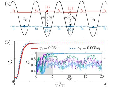
Figure 1: (a) Atomic lattice as described in main text. (b) Emergent synchronization. Main panel: Global SS $\mathcal{C}_{T}(t=10/\gamma_{1})$ as a function of $\gamma_{1}/\gamma_{2}$ for two different rates $\gamma_{1}$. Inset: Evolution of $\mathcal{C}_{\langle\hat{\sigma}^{x}_{j}\rangle,\langle\hat{\sigma}^{x}_{j+1}\rangle}$ for $j=1$ (purple line), $j=2$ (in green), and $j=3$ (in blue), with $\omega_{1}\Delta t=3$. Here $\gamma_{1}/\omega_{1}=0.05$, solid lines correspond to $\gamma_{1}=4\gamma_{2}$ (staggered losses), dotted lines to $\gamma_{1}=\gamma_{2}$ (homogeneous losses). Shadowed region displays the transient after which the staggered case displays synchronization. System of $N=4$ spins, $\delta=0.75\omega_{1}$, $\lambda=0.4\omega_{1}$, initial state $|\Psi(t=0)\rangle=|+\rangle_{1}\otimes|+\rangle_{2}\otimes|+\rangle_{3}\otimes|+\rangle_{4}$, where $|+\rangle_{j}=(|0\rangle+|\{1\}_{j}\rangle)/\sqrt{2}$ and $|\{1\}_{j}\rangle$ means spin $j$ excited, the rest in vacuum.

Using standard techniques to produce double wells 2well , the dissipative model of giedke can be modified such that the lattice results in dimer arrangement where, in each well, the motional states have different (staggered) energy separation $\tilde{\omega}_{1,2}$ (Fig. 1a). Provided that the modulation of the optical wells can be treated as a perturbation, a dimer effective spin model can be obtained (further details in SupplementalMaterial ) with Hamiltonian ($\hbar=1$):

$$\hat{H}=\sum_{j=1}^{N}\frac{\omega_{j}}{2}\hat{\sigma}^{z}_{j}+\sum_{j=1}^{N-1}\lambda(\hat{\sigma}^{+}_{j}\hat{\sigma}^{-}_{j+1}+h.c.),$$ (1)

where $\omega_{j}=\omega_{1(2)}$ if $j$ is odd (even), $\omega_{j}=\tilde{\omega}_{j}-\omega_{0}$, $\omega_{0}$ is the central large frequency and $\lambda$ is the spin-spin coupling. These parameters satisfy $\omega_{0}\gg\omega_{1,2},\delta,\lambda$, where $\delta=\omega_{1}-\omega_{2}$ is the detuning between the two sublattices.

The use of a bichromatic lattice will also affect the engineered dissipation, as the corresponding decay rates also depend on the trap frequency through detuning with the cooling laser giedke . In the weak dissipation regime, the reduced density matrix $\hat{\rho}$ of the chain obeys a standard master equation GKSL $\partial_{t}\hat{\rho}(t)=\mathcal{L}\hat{\rho}(t)$, with Liouvillian $\mathcal{L}\,\cdot=i[\cdot,\hat{H}]+\sum_{j}\gamma_{j}(2\hat{\sigma}^{-}_{j}\,\cdot\,\hat{\sigma}^{+}_{j}-\{\cdot,\hat{\sigma}^{+}_{j}\hat{\sigma}^{-}_{j}\})$. Because of the presence of a bichromatic lattice, the decay rates $\gamma_{j}$ also assume staggered values and can be chosen such that $\gamma_{1}/\omega_{1}=\gamma_{2}/\omega_{2}$ SupplementalMaterial .

A key observation for the analysis of the dynamics is that the whole eigenvalue spectrum of ${\cal L}$ can be analytically determined observing that it coincides with the one of $\mathcal{K}$, which is defined through $\partial_{t}\hat{\rho}(t)=-i(\hat{K}\hat{\rho}(t)-\hat{\rho}(t)\hat{K}^{\dagger})\equiv{\mathcal{K}}\hat{\rho}(t)$ and is obtained by replacing $\hat{H}$ with the non-Hermitian Hamiltonian $\hat{K}=\hat{H}-i\sum_{j}^{N}\gamma_{j}\hat{\sigma}^{+}_{j}\hat{\sigma}_{j}^{-}$ and by neglecting the jump operators $\hat{\sigma}^{-}_{j}\,\hat{\rho}\,\hat{\sigma}^{+}_{j}$. In fact, in the eigenbasis of $\mathcal{K}$, $\mathcal{L}$ has an upper triangular form in which the diagonal elements are the eigenvalues of $\mathcal{K}$ (and then of $\mathcal{L}$ itself) and the non-local jump operators only contribute to off-diagonal elements (see Ref. Mauricio for a detailed discussion).

Diagonalization of $\hat{K}$ via Jordan-Wigner transformation and Fourier transform leads to the two-band elementary complex eigenvalues SupplementalMaterial

$$\Omega^{\pm}_{k}=\frac{\Omega_{1}+\Omega_{2}}{2}\pm\frac{1}{2}\sqrt{(\Omega_{1}-\Omega_{2})^{2}+16\lambda^{2}\,\text{cos}^{2}\frac{k}{2}},$$ (2)

and conjugates $\Omega_{k}^{\pm*}$ for $\hat{K}^{\dagger}$, where we assumed open boundary conditions, with $k=2\pi l/(N+1)$, $l=1,2,...,N/2$ and

$$\Omega_{1(2)}=\omega_{1(2)}-i\gamma_{1(2)}.$$ (3)

The eigenvalues of $\mathcal{L}$ are obtained by combining $\Omega_{k}^{\pm}$ and $\Omega_{k}^{\pm*}$ as prescribed in Mauricio , such that their imaginary part (decay rates) always add together. Moreover, $-i\Omega_{k}^{\pm}$ and $i\Omega_{k}^{\pm*}$ are already eigenvalues of $\mathcal{L}$, corresponding to one-excitation eigenmodes. Thus, the smallest decay rates of the system belong to this sector. As a consequence, the relaxation dynamics before the final decay into the vacuum state is conveniently described in the one-excitation sector, considering the slowest modes that can be identified comparing their decay rates $\Gamma_{l}$ (absolute value of the imaginary parts of $\Omega_{k}^{\pm}$) and frequencies $\nu_{l}$ (real parts of $\Omega_{k}^{\pm}$) ordering .

Synchronization by staggered losses.– We analyze the the full system dynamics and quantify the emergence of SS among atomic observables with no classical counterpart, as the spin coherences $\langle\hat{\sigma}^{x}_{j}\rangle$ ZambriniRev . Indeed at any time during relaxation, coherences are present before reaching the equilibrium vacuum state. Their dynamical synchronization can be assessed by a Pearson correlation parameter $\mathcal{C}$ ZambriniRev , a common measure of synchronization between temporal trajectories, $x_{1(2)}(t)$, defined as $\mathcal{C}_{x_{1},x_{2}}(t)=\overline{\delta x_{1}\delta x_{2}}/\sqrt{\overline{\delta x_{1}^{2}}\,\,\overline{\delta x_{2}^{2}}}$, averaging on a time window $\Delta t$ of few oscillations $\overline{x_{j}}=\frac{1}{\Delta t}\int_{t}^{t+\Delta t}ds\,x_{j}(s)$, and $\delta x_{j}=x_{j}-\overline{x_{j}}$. Delayed synchronization is accounted considering the correlation at different times, $x_{1}(t)$ and $x_{2}(t+\tau)$, and maximizing over $\tau$, in general numerically, as for results presented in Fig. 1b. In Fig. 1b (inset) we show $\mathcal{C}_{\langle\hat{\sigma}^{x}_{j}\rangle,\langle\hat{\sigma}^{x}_{j^{\prime}}\rangle}(t)$ among nearest-neighbor spin pairs, ranging between $0$ (no SS) to $1$ (perfect SS): synchronization is found among all atoms in the presence of local staggered dissipation (solid lines), while it does not emerge for $\gamma_{1}=\gamma_{2}$ (dotted lines). We also consider the global SS indicator $\mathcal{C}_{T}(t)=\prod_{i<j}\mathcal{C}_{\langle\hat{\sigma}^{x}_{i}\rangle,\langle\hat{\sigma}^{x}_{j}\rangle}(t)$ (main panel of Fig. 1b) reaching its maximum value $1$ only if all atom coherences are synchronized. We see that SS for a given detuning ($\delta=0.75\omega_{1}$ in Fig. 1b) is enabled by the presence of staggered dissipation rates, emerging for a wide range of $\gamma_{1}/\gamma_{2}$ values, while it disappears if losses become uniform ($\gamma_{1}/\gamma_{2}\approx 1$).

The emergence of SS is due the presence of multiple dissipative time scales, as occurs in other models manzanoSciRep ; GLG1 ; GLG2 ; Bellomo . Normal modes can conjure to dissipate at widely different rates, $\Gamma_{l}$, so that the predominant contribution to the long-time dynamics is represented by the slowest decaying mode. Quantum SS then emerges as an ordered, spatially delocalized, monochromatic oscillation in the pre-asymptotic regime (transient synchronization). This is the case when considering our lattice with staggered dissipation, as revealed by inspection of the Liouvillian spectrum. On the other hand, if local dissipation is spatially homogeneous, the imaginary parts of the eigenvalues (S19) coincide, there is no separation between decay rates, and in fact the system does not synchronize in spite of the presence of coherent coupling between spins (Fig. 1b).

Inter-band and intra-band synchronization.– The ability of the system to synchronize relies on the interplay between different parameters whose assessment can be conveniently limited to the one-excitation sector of $\mathcal{L}$. Synchronization of the whole chain is calculated at a time long enough to wash out the presence of the slowest modes, in Fig. 2a, as a function of the spin-spin coupling $\lambda$ and the detuning $\delta$, for a short chain of four spins. This SS map shows a non-trivial scenario with two different and well separated regions that support SS, both occurring for strong detuning (yellow regions): region I characterized by strong coupling, and region II, by small coupling and a larger detuning window.

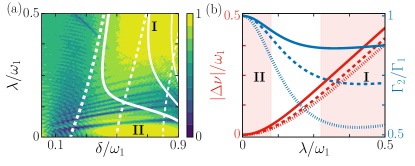
Figure 2: (Color online) (a) Map of SS among all spin pairs $\mathcal{C}_{T}(t)$ at $\gamma_{1}t=10$ and $\omega_{1}\Delta t=80$, varying detuning and coupling strength, with $|\Psi(t=0)\rangle=|0\rangle/\sqrt{2}+(|\{1\}_{2}\rangle+|\{1\}_{3}\rangle)/2$. Strong SS is found at the yellow (light color) regions I and II ($\mathcal{C}_{T}\geq 0.9$). White lines are contours of the ratio of the two smallest decay rates, $\Gamma_{2}/\Gamma_{1}$ (solid lines), and of the smallest decay rates of each band $\Gamma_{2}/\Gamma_{3}$ (dashed lines). Thicker lines for increasing ratio values, respectively $(0.9,0.75,0.6)$ and $(0.8,0.5,0.2)$. (b) In red, difference between the frequencies associated to the smallest decay rates: $|\Delta\nu|=|\nu_{1}-\nu_{2}|$, varying $\lambda$. In blue, ratio between the smallest decay rates. Solid lines $\delta=0.5\omega_{1}$, dashed lines $\delta=0.75\omega_{1}$, dotted lines $\delta=0.9\omega_{1}$. For both figures $\gamma_{j}=0.05\omega_{j}$.

These SS regimes can be understood analyzing the spectral content of the coherences’ dynamics in the one-excitation sector $\langle\hat{\sigma}^{x}_{j}(t)\rangle=2Re\big{[}\sum_{l=1}^{4}u_{l}(j)e^{-(i\nu_{l}+\Gamma_{l})t}\big{]}$, with weights $u_{l}(j)$ depending on the site $j$, eigenmode $l$, and initial condition SupplementalMaterial . In region II the frequencies are nearly degenerate in each ($\pm$) band, while $N$ well separated frequencies are present in region I.

The “flat” and well separated two-band spectrum found in region II leads to what we term inter-band synchronization. In fact, in the limit of vanishing $\lambda$, the two frequency degenerate bands (Fig. 2b) are separated by $\delta+i(\gamma_{1}-\gamma_{2})$. For weak coupling $\lambda$, two manifolds emerge with very similar frequencies and damping rates. Each of the sublattices of the atomic dimer is strongly coupled to one of the manifolds and weakly coupled to the other one, leading to an effective two-body behavior reminiscent of the mean-field scenario described in SyncAtomicEnsemb ; SyncDipoles . Inter-band SS is present as long as the difference in local losses $\gamma_{1,2}$ allows one to establish two well separated time scales (region highlighted by white dashed lines in Fig. 2a). Being the staggered damping rates related to the sublattices detuning (here we consider $\gamma_{1}/\omega_{1}=\gamma_{2}/\omega_{2}$), SS only emerges for detuning $\delta$ larger than a threshold value, at difference from the typical scenario of SS favored by small detuning ClassSync and similarly to synchronization blockade lorch ; GLG2 . This region shrinks when decreasing dissipation strength $\gamma_{j}$ as shown in SupplementalMaterial .

Increasing the coupling $\lambda$, SS deteriorates (Fig. 2a, $0.1\lesssim\lambda/\omega_{1}\lesssim 0.25$) as the two-body behavior disappears and several non-degenerate modes compete. Synchronization is restored for coupling strengths such that there is a significant difference between the two slowest dissipation rates, now in the lower band, so that a leading mode governs the long-time dynamics. This is intra-band synchronization occurring in region I and requiring significant deviations between the slowest dissipation rates (as highlighted by white solid lines in Fig. 2a). This picture is confirmed when looking at the two slowest modes in Fig. 2b, with frequencies and decay rates of the lower band drifting apart as the coupling increases.

When considering longer chains, the two physical mechanisms I and II for SS imply different levels of robustness. In fact, inter-band synchronization II persists for long chains, as it mainly relies on the presence of the gap $\delta+i(\gamma_{1}-\gamma_{2})$. This is not the case of region I, where the relevant spectral gap is obtained taking the difference between the two values of $\Omega^{-}_{k}$ with the smallest imaginary parts, which goes to zero as $N$ increases, Eq. (S19). Furthermore, the simultaneous participation of all the eigenmodes of the lower band, makes the synchronized phase in region II almost spatially homogeneous, while the predominance of a single mode in region I determines a nontrivial spatial structure, which also contributes to the loss of global synchronization as size increases SupplementalMaterial .

Synchronization measures.– Often, two-body quantum correlation indicators are taken as bona fide synchronization measures ZambriniRev , as they are able to reveal the presence of phase locking. Here, we show that the presence of such correlations is necessary but not sufficient to predict the emergence of SS. We study the one-time correlation $Z(t)\equiv\langle\hat{\sigma}^{x}_{1}(t)\hat{\sigma}^{x}_{2}({t})\rangle$ often considered in the context of superradiance gross , where $t$ is set after the onset of SS. As shown in Fig. 3a, $Z$ increases with detuning (analogous results are found for other pairs) but it displays a weak dependence on $\lambda$, being then unable to capture the transition from region I to region II. An explanation can be given considering the one-excitation sector where $Z(t)=2Re[\langle\hat{\sigma}^{+}_{1}(t)\hat{\sigma}^{-}_{2}(t)\rangle]$ hence $Z(t)=2Re[\sum_{l,m=1}^{4}w_{l,m}(1,2)e^{[-i(\nu_{l}-\nu_{m})-\Gamma_{m}-\Gamma_{l}]t}]$, with weights $w_{l,m}(1,2)$ depending on the spins, eigenmodes $l$ and $m$, and initial condition SupplementalMaterial . The evolution of $Z$ is governed by exponentials containing combinations of eigenvalues instead of single ones, depending then on slow and less slow rates. Therefore, differently from $\mathcal{C}$, it does not allow to distinguish the slowest relaxation modes.

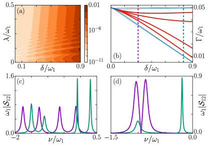
Figure 3: (a) In color $|Z(\bar{t})|$, with $\gamma_{1}\bar{t}=10$, $|\Psi(t=0)\rangle=|0\rangle/\sqrt{2}+\sum_{j=1}^{4}|\{1\}_{j}\rangle/\sqrt{8}$, and averaged over few oscillations. We plot the absolute value as the magnitude of the correlations is the relevant quantity. (b) Decay rates $\Gamma_{l}$ as a function of the detuning, for $\lambda=0.5\omega_{1}$ (red) and $\lambda=0.05\omega_{1}$ (blue). (c,d) $\omega_{1}|\mathcal{S}_{12}(\nu/\omega_{1})|$, with $\delta=0.1\omega_{1}$ (purple) and $\delta=0.8\omega_{1}$ (green). In (c) we fix $\lambda=0.5\omega_{1}$ (SS I), and in (d) $\lambda=0.05\omega_{1}$ (SS II). We plot the absolute values to ease peak comparison. In all plots $\gamma_{j}/\omega_{j}=0.05$.

Different is the case for two-time correlation functions of the type $\langle\hat{\sigma}^{-}_{l}(t+\tau)\hat{\sigma}^{+}_{m}(t)\rangle$ in the stationary state, related to absorption spectra GambettaPRA2006 (for emission of radiating dipoles see Refs.SyncAtomicEnsemb ; SyncDipoles ). These are found to capture the presence of SS in both regimes I and II described above. In Fig. 3c,d we plot $\mathcal{S}_{12}(\nu)=Re\big{[}\frac{1}{2\pi}\int_{0}^{\infty}d\tau e^{-i\nu\tau}\langle\hat{\sigma}^{-}_{1}(\tau)\hat{\sigma}^{+}_{2}(0)\rangle\big{]}$ in the (vacuum) stationary state of the system. In the one excitation sector we obtain $\langle\hat{\sigma}^{-}_{1}(\tau)\hat{\sigma}^{+}_{2}(0)\rangle=\sum_{l=1}^{4}v_{l}(1,2)e^{-(i\nu_{l}+\Gamma_{l})\tau}$, with weights $v_{l}(1,2)$ depending on the overlap of the eigenmode with the considered spin sites SupplementalMaterial . We observe that the dynamics of these correlation functions is the same as the one for the spin coherences (with the initial condition $\hat{\sigma}_{j}^{+}|0\rangle$), in agreement with the quantum regression theorem Carmichael . Thus the spectra $\mathcal{S}_{lm}(\nu)$ for each pair $l,m$ display a set of at most $N$ resonance peaks, localized at the eigenfrequencies of the one-excitation sector, with linewidths determined by the corresponding decay rates, and height depending on the weights $v_{l}(1,2)$. This spectra contain the information needed for the analysis of SS.

In Fig. 3c we plot a synchronized (green line) and an unsynchronized (purple line) two-time correlation function for strong coupling, while in Fig. 3d we do it for weak coupling. In the absence of SS, for small detuning and strong coupling (Fig. 3c), the spectrum displays multiple peaks, no one significantly sharper than the others. For both small detuning and coupling, we find two peaks with similar decay rates (Fig. 3d), while in the no-SS region between region I and II of Fig. 2a two of the four peaks (the ones of the same band) display similar width SupplementalMaterial . Looking instead at SS parameter regions, the spectra are characterized by the presence of a peak with width significantly smaller than the rest. Intra-band synchronization (I) in Fig. 3c displays a sharper third line among four, while in Fig. 3d, inter-band SS (II) clearly shows the effective two-body behavior of the system discussed above. This is also appreciated in Fig. 3b where, for small coupling (blue lines), two pairs of nearly degenerate decay rates emerge as detuning is increased. In contrast, for strong coupling (red lines), the system displays four well-differentiated decay rates. For both strong and weak coupling as detuning grows one of the peaks becomes significantly thinner, transiting from the purple spectra in Fig. 3c,d to the green ones SupplementalMaterial . These correlations, in the case of stationary synchronization reported in Ref. SyncAtomicEnsemb , are characterized by the presence of a single peak in the spectrum, a situation never occurring in our system for $\gamma_{1}/\gamma_{2}=\omega_{1}/\omega_{2}$.

Conclusions.– We have shown quantum spontaneous synchronization of an XX dissipative model in dimeric spin chain that can be simulated in atomic lattices giedke , and other set-ups. Differently from other atomic systems, SS is enabled by spatial modulation of local losses, without any collective dissipation, and disappears in the homogeneous limit. We have identified two SS regimes, interpreted in terms of the Liouvillian spectrum of the dynamics, and shown that inter-band SS is robust in long chains while intra-band SS tends to disappear. We have analyzed the use of spin-spin correlations to assess the emergence of SS, comparing equal-time and two-time correlations. While showing the limitations of the former, two-time correlation functions are found to properly demarcate the different regimes of transient (as well as stationary SyncAtomicEnsemb ) synchronization, looking at the number, position and width of the peaks. Beyond the experimental realization of SS in atomic lattices as proposed here, future interesting directions are the generalization of the proposed atomic set-up to display other forms of synchronization and the connection of this phenomenon with timely concepts such as time-crystals and coalescence.

Acknowledgements.– The authors acknowledge support from the Horizon 2020 EU collaborative project QuProCS (Grant Agreement No. 641277), MINECO/AEI/FEDER through projects EPheQuCS FIS2016-78010-P, CSIC Research Platform PTI-001, the María de Maeztu Program for Units of Excellence in R$\&$D (MDM-2017-0711), and funding from CAIB PhD and postdoctoral programs.

Supplemental Material: ’Quantum synchronization in dimer atomic lattices’

S1 Dissipative atomic lattice

In this section the main details on the physical implementation of the dissipative spin chain are overviewed. In S1.1 we present the Hamiltonian that models the atomic lattice. We follow in S1.2 explaining how from this atomic lattice one can realize effective spin Hamiltonians. In S1.3 we comment on the proposed dissipation scheme of Ref. S_SpinDiss , while we end in S1.4 discussing briefly typical numerical values for the parameters of the atomic system.

S1.1 Two band Bose-Hubbard model

We consider a system of bosonic atoms in the Mott-insulator regime (MI), trapped in the two lowest energy bands of a bichromatic optical lattice. The optical lattice is assumed to be strongly anharmonic, such that higher vibrational levels are not populated. The system is described by the following two-band Bose-Hubbard Hamiltonian:

$$\hat{H}_{BH}=\hat{H}_{0}+\hat{H}_{1}+\hat{H}_{t}.$$ (S1)

The different contributions to this Hamiltonian are the following. $\hat{H}_{0}$ describes the atom-atom repulsive interactions and the unperturbed optical potential ($\hbar=1$) S_SpinDiss :

$$\begin{split}\hat{H}_{0}=\sum_{j=1}^{N}\bigg{\{}\frac{\omega_{0}}{2}(\hat{d}^{\dagger}_{j}\hat{d}_{j}-\hat{c}^{\dagger}_{j}\hat{c}_{j})+U_{01}\hat{c}^{\dagger}_{j}\hat{c}_{j}\hat{d}^{\dagger}_{j}\hat{d}_{j}\\ +\frac{U_{00}}{2}\hat{c}^{\dagger}_{j}\hat{c}_{j}(\hat{c}^{\dagger}_{j}\hat{c}_{j}-1)+\frac{U_{11}}{2}\hat{d}^{\dagger}_{j}\hat{d}_{j}(\hat{d}^{\dagger}_{j}\hat{d}_{j}-1)\bigg{\}},\end{split}$$ (S2)

$\hat{H}_{1}$ contains the small modulations to the optical potential:

$$\hat{H}_{1}=\sum_{j\in\text{odd}}\frac{\omega_{1}}{2}(\hat{d}^{\dagger}_{j}\hat{d}_{j}-\hat{c}^{\dagger}_{j}\hat{c}_{j})+\sum_{j\in\text{even}}\frac{\omega_{2}}{2}(\hat{d}^{\dagger}_{j}\hat{d}_{j}-\hat{c}^{\dagger}_{j}\hat{c}_{j}),$$ (S3)

and $\hat{H}_{t}$ the perturbative tunneling processes between neighboring sites:

$$\hat{H}_{t}=\sum_{j=1}^{N-1}(t_{0}\hat{c}^{\dagger}_{j}\hat{c}_{j+1}+t_{1}\hat{d}^{\dagger}_{j}\hat{d}_{j+1}+H.c.).$$ (S4)

The bosonic operators $\hat{c}_{j}^{\dagger}$ and $\hat{c}_{j}$ ($\hat{d}_{j}^{\dagger}$ and $\hat{d}_{j}$) create and annihilate an atom in the lowest (second lowest) motional state of site $j$ of the optical lattice. As in S_SpinDiss the only atom-atom interactions are given by the same site and same motional state repulsion energies $U_{00}$ and $U_{11}$, and the same site different motional state repulsion $U_{01}$. Tunneling between neighboring sites without exchange of the motional state is permitted, with rates $t_{0}$ and $t_{1}$ S_SpinDiss . Finally the motional states are separated by a large energy $\omega_{0}$ with small dimeric modulations $\omega_{1}$ and $\omega_{2}$. We consider the system to be in a regime in which there is one atom per site. We recall the usual hierarchy of parameter values that ensures the validity of the model S_Jaksch1 ; S_Jaksch2 ; S_SpinDiss :

$$\omega_{0}\gg U_{00},U_{11},U_{01}\gg t_{0},t_{1}.$$ (S5)

Notice that as we consider small frequency modulations of the optical potential, we must also require that:

$$\omega_{0}\gg\omega_{1},\omega_{2},\quad U_{00},U_{11},U_{01}\gg\delta,$$ (S6)

with $\delta=\omega_{1}-\omega_{2}$. The first condition is necessary to be able to treat the modulations of the potential as a perturbation to the monochromatic Hamiltonian (S2). The second additional condition is instead necessary to obtain the desired effective spin Hamiltonian (see next subsection).

S1.2 Effective spin Hamiltonian

An important observation is that $\hat{H}_{BH}$, besides conserving the total number of atoms $n$, also conserves the total number of atoms in each motional state $n_{0}$ and $n_{1}$. Hence, the eigenstates of $\hat{H}_{0}+\hat{H}_{1}$ are given by the possible ways to distribute $n$ atoms in the two motional states of the optical lattice. Here we are interested in the low energy sector of the case $n=N$, in which there is one atom per site. In fact for prescribed values of $n_{0}$ and $n_{1}$, the lowest energy eigenstates, i.e. the ones with an atom per site, form a manifold of states with intra-energy separation of the order of $\delta$. In turn, all possible configurations in which there is one site with two atoms, form also a manifold with intra-energy separation again of order $\delta$. Both manifolds are separated by an energy gap of order of the repulsive interactions and hence much larger than the intra-manifold energy scales (Eq. (S6)). When considering $\hat{H}_{t}$, only matrix elements between unperturbed states of different manifold are non-zero. Then, if one is interested in the low energy physics of the system, one can use perturbation theory to obtain an effective Hamiltonian for the lowest energy manifold, and further neglect all states with more than one atom per site S_Cohen . In this Schrieffer-Wolff kind of approach S_SpinDiss ; S_Spins2 ; S_Spins3 ; S_Spins4 , second order tunneling processes couple the lowest energy states by means of virtual transitions to states with two atoms per site, which are energetically unfavorable. Thus to second order, one obtains the following effective Hamiltonian governing the manifold of states with one atom per site:

$$\begin{split}\hat{H}_{\text{eff}}=\sum_{j=1}^{N-1}\bigg{\{}C_{1}\,\hat{c}_{j}^{\dagger}\hat{c}_{j}\hat{c}_{j+1}^{\dagger}\hat{c}_{j+1}+C_{2}\,\hat{d}_{j}^{\dagger}\hat{d}_{j}\hat{d}_{j+1}^{\dagger}\hat{d}_{j+1}\\ +C_{3}\,(\hat{c}_{j}^{\dagger}\hat{c}_{j+1}\hat{d}_{j+1}^{\dagger}\hat{d}_{j}+\hat{d}_{j}^{\dagger}\hat{d}_{j+1}\hat{c}_{j+1}^{\dagger}\hat{c}_{j})\\ +C_{4}\,\hat{c}_{j}^{\dagger}\hat{c}_{j}\hat{d}_{j+1}^{\dagger}\hat{d}_{j+1}+C_{5}\,\hat{d}_{j}^{\dagger}\hat{d}_{j}\hat{c}_{j+1}^{\dagger}\hat{c}_{j+1}\bigg{\}}\\ +\sum_{j\in\text{odd}}\big{(}\frac{\omega_{0}+\omega_{1}}{2}\big{)}(\hat{d}^{\dagger}_{j}\hat{d}_{j}-\hat{c}^{\dagger}_{j}\hat{c}_{j})\\ +\sum_{j\in\text{even}}\big{(}\frac{\omega_{0}+\omega_{2}}{2}\big{)}(\hat{d}^{\dagger}_{j}\hat{d}_{j}-\hat{c}^{\dagger}_{j}\hat{c}_{j}),\end{split}$$ (S7)

with the coefficients taking the following values:

$$\begin{split}C_{1}=-\frac{t_{0}^{2}}{U_{00}-\delta}-\frac{t_{0}^{2}}{U_{00}+\delta}\approx-\frac{2t_{0}^{2}}{U_{00}},\\ C_{2}=-\frac{t_{1}^{2}}{U_{11}-\delta}-\frac{t_{1}^{2}}{U_{11}+\delta}\approx-\frac{2t_{1}^{2}}{U_{11}},\\ C_{3}=-\frac{t_{0}t_{1}}{U_{01}-\delta}-\frac{t_{0}t_{1}}{U_{01}-\delta}\approx-\frac{2t_{0}t_{1}}{U_{01}},\\ C_{4}=-\frac{t_{0}^{2}+t_{1}^{2}}{U_{01}-\delta},\quad C_{5}=-\frac{t_{1}^{2}+t_{0}^{2}}{U_{01}+\delta},\\ C_{4}\approx C_{5}\approx-\frac{t_{0}^{2}+t_{1}^{2}}{U_{01}}.\end{split}$$ (S8)

Notice that in (S8) we make use of the condition (S6) to further approximate the expression of the coefficients. We can now define the spin states $\hat{c}^{\dagger}_{j}|0_{j}\rangle=|\downarrow_{j}\rangle$ and $\hat{d}^{\dagger}_{j}|0_{j}\rangle=|\uparrow_{j}\rangle$, together with the proper spin operators:

$$\begin{split}\hat{\sigma}_{j}^{+}=\hat{d}_{j}^{\dagger}\hat{c}_{j},\quad\hat{\sigma}_{j}^{-}=\hat{c}_{j}^{\dagger}\hat{d}_{j},\\ \hat{\sigma}_{j}^{z}=\hat{d}^{\dagger}_{j}\hat{d}_{j}-\hat{c}^{\dagger}_{j}\hat{c}_{j},\\ \mathbb{1}_{2\times 2}=\hat{d}^{\dagger}_{j}\hat{d}_{j}+\hat{c}^{\dagger}_{j}\hat{c}_{j},\end{split}$$ (S9)

thus obtaining the following effective spin Hamiltonian:

$$\begin{split}\hat{H}_{\text{spin}}=\sum_{j=1}^{N-1}\big{\{}\lambda(\hat{\sigma}_{j}^{+}\hat{\sigma}_{j+1}^{-}+\hat{\sigma}_{j+1}^{+}\hat{\sigma}_{j}^{-})+\lambda_{z}\hat{\sigma}_{j}^{z}\hat{\sigma}_{j+1}^{z}\big{\}}\\ +\sum_{j\in\text{odd}}\bigg{(}\frac{\omega_{0}+\omega_{1}}{2}+h_{z}\bigg{)}\hat{\sigma}_{j}^{z}+\sum_{j\in\text{even}}\bigg{(}\frac{\omega_{0}+\omega_{2}}{2}+h_{z}\bigg{)}\hat{\sigma}_{j}^{z}.\end{split}$$ (S10)

with the parameters defined as:

$$\begin{split}\lambda\approx-\frac{2t_{0}t_{1}}{U_{01}},\quad h_{z}\approx\frac{1}{2}\bigg{(}\frac{t_{0}^{2}}{U_{00}}-\frac{t_{1}^{2}}{U_{11}}\bigg{)},\\ \lambda_{z}\approx-\frac{1}{2}\bigg{(}\frac{t_{0}^{2}}{U_{00}}+\frac{t_{1}^{2}}{U_{11}}-\frac{t_{0}^{2}+t_{1}^{2}}{U_{01}}\bigg{)}.\end{split}$$ (S11)

Finally, $\hat{H}$ of Eq. (1) in the main text corresponds to parameters of the optical lattice such that $\lambda_{z}=0$. Then $\hat{H}$ is $\hat{H}_{\text{spin}}$ in a frame rotating with $\frac{\omega_{0}}{2}+h_{z}$.

S1.3 Engineered dissipation

A detailed derivation of the dissipation scheme used in this work is found in Ref. S_SpinDiss and here we review the main conditions to implement it. It is assumed that the atoms are in the Lamb-Dicke regime ($\eta_{j}\ll 1$, where $\eta_{j}$ is the Lamb-Dicke parameter at site $j$) and have a ‘$\Lambda$’ internal structure with two ground states. By means of weak off-resonant Raman transitions the excited state is adiabatically eliminated, leading to an effective two level system with tunable decay rates S_SpinDiss ; S_cooling2 ; S_cooling3 . This effective two-level system is characterized by an effective Rabi frequency $\Omega_{\text{eff}}$, an effective detuning $\delta_{r}$, an effective decay rate $\Gamma$, and an effective dephasing rate $\gamma$, where the expression for these parameters is found in many references S_SpinDiss ; S_cooling2 ; S_cooling3 . The parameters are then adjusted so that the two-level system resolves the motional degrees of freedom, i.e. $\Gamma+\gamma\ll\tilde{\omega}_{j}$ (with $\tilde{\omega}_{j}=\omega_{0}+\omega_{j}$) S_SpinDiss ; S_cooling2 ; S_cooling3 . Finally, if $\eta_{j}|\Omega_{\text{eff}}|\ll\Gamma,\gamma,|\delta_{r}|,\tilde{\omega}_{j}$ S_SpinDiss , the parameter regime is characterized by weak coupling of internal and motional degrees of freedom, and one can adiabatically eliminate the former obtaining an effective master equation for the motional degrees of freedom S_cooling1 . Under the appropriate resonance conditions, heating can be neglected, and one obtains that the density matrix evolves according to the Liouvillian $\mathcal{L}\,\cdot=i[\cdot,\hat{H}]+\sum_{j}\gamma_{j}(2\hat{\sigma}^{-}_{j}\,\cdot\,\hat{\sigma}^{+}_{j}-\{\cdot,\hat{\sigma}^{+}_{j}\hat{\sigma}^{-}_{j}\})$ with motional decay rate:

$$\gamma_{j}=\eta_{j}^{2}\Omega_{\text{eff}}^{2}\frac{\Gamma+\gamma}{(\Gamma+\gamma)^{2}+(\delta_{r}-\tilde{\omega}_{j})^{2}}.$$ (S12)

Notice that, in order to suppress heating, the effective detuning should be tuned close to the large mechanical energy, i.e. $\delta_{r}\sim\omega_{0}$. Then the dependence of the decay rate on the lattice site comes mainly from the resonance frequency of the Lorentzian, as differences between $\eta_{1}^{2}$ and $\eta_{2}^{2}$ are of the order of $\omega_{j}/\omega_{0}\ll 1$. Defining $\epsilon=\delta_{r}-\omega_{0}\sim|\omega_{j}|$ (which can be positive or negative), and by properly adjusting it, the decay rates can in general take staggered values. Furthermore, besides implementing staggered decay rates by means of the effective detuning (as described here), different approaches are also proposed in S_SpinDiss , as for example by tuning the phase difference between two cooling lasers.

S1.4 Brief survey of parameter values

We follow references S_Jaksch1 ; S_Jaksch2 to illustrate the values that the parameters of this system can take. For sodium atoms in a blue detuned optical trap of wavelength $\lambda_{T}=514$nm, the recoil energy is $E_{R}=2\pi\times 33$kHz. Tuning the light intensity, the energy separation between the two lowest energy motional states of the lattice can be fixed to $\omega_{0}\sim 1$MHz, which leads to $U_{lm}\sim 40$kHz and $t_{l}\sim 4$kHz ($l,m=0,1$). In these conditions the atomic chain is in the MI regime with one atom per site. Moreover, according to eq. S11, $\lambda\sim 0.8$kHz which sets the order of magnitude of the small modulations $\omega_{j}$, as we take $\omega_{j}\sim\lambda$ in all the work. Considering possible sources of dissipation, we notice that in the MI regime with one atom per site atom-atom collisions are strongly suppressed S_Jaksch1 . In addition, for these parameter values, the rate of dissipation due to the optical potential can be estimated to be of the order of $10^{-2}$Hz S_Jaksch2 , and we neglect it. This last approximation is consistent with the much larger values that we have fixed for the engineered decay rates, $\gamma_{j}$, which we estimate to be in the range $\sim 1-40$Hz.

S2 Liouvillian spectrum

As it is shown in Ref. S_Mauricio , the eigenvalues of the type of Liouvillian $\mathcal{L}$ considered here, are prescribed linear combinations of those of the non-Hermitian Hamiltonian $\hat{K}=\hat{H}-i\sum_{j}^{N}\gamma_{j}\hat{\sigma}^{+}_{j}\hat{\sigma}_{j}^{-}$. In fact, as commented in the main text, the eigenvalues with the smallest decay rates coincide with eigenvalues of $\hat{K}$ and their complex conjugates. Thus in order to characterize the long-time relaxation dynamics we need to diagonalize $\hat{K}$. To do so we use the Jordan-Wigner transformation to work with fermions instead of spins:

$$\begin{split}\hat{\sigma}^{z}_{j}=2\hat{f}^{\dagger}_{j}\hat{f}_{j}-1,\\ \hat{\sigma}^{+}_{j}=\hat{f}^{\dagger}_{j}e^{i\hat{\phi}_{j}},\quad\hat{\sigma}^{-}_{j}=\hat{f}_{j}e^{-i\hat{\phi}_{j}},\\ \hat{\phi}_{j}=\pi\sum_{l<j}\hat{n}_{l},\end{split}$$ (S13)

where $\hat{f}_{j}^{\dagger}(\hat{f}_{j})$, $\hat{n}_{j}=\hat{f}_{j}^{\dagger}\hat{f}_{j}$, are the creation (annihilation) and number fermionic operators of site $j$. Then defining $\Omega_{1(2)}=\omega_{1(2)}-i\gamma_{1(2)}$, and using a notation that displays explicitly the dimeric character of the chain, we obtain the fermionic non-Hermitian Hamiltonian:

$$\begin{split}\hat{K}_{F}=\sum_{j=1}^{N/2}\Omega_{1}\hat{a}^{\dagger}_{j}\hat{a}_{j}+\sum_{j=1}^{N/2}\Omega_{2}\hat{b}^{\dagger}_{j}\hat{b}_{j}\\ +\sum_{j=2}^{N/2}\lambda(\hat{a}^{\dagger}_{j}\hat{b}_{j-1}+H.c)+\sum_{j=1}^{N/2}\lambda(\hat{a}^{\dagger}_{j}\hat{b}_{j}+H.c.),\end{split}$$ (S14)

where now $\hat{a}_{j}^{\dagger}(\hat{a}_{j})$ and $\hat{b}_{j}^{\dagger}(\hat{b}_{j})$ are fermionic creation (annihilation) operators of site $j$ and its basis, respectively. The diagonalization of $\hat{K}_{F}$ is accomplished in two steps: first we diagonalize the system assuming periodic boundary conditions, and later we combine the obtained eigenstates to find the ones of the open boundary case. In the following we write the main results of each step.

S2.1 Periodic boundary conditions

In this case the summation in the third term of Eq. (S14) starts from $j=1$, and the boundary conditions imply that $\hat{a}_{0}=\hat{a}_{N/2}$ and $\hat{b}_{0}=\hat{b}_{N/2}$. We define $M=N/2$ and relabel the index $j$ to run from $j=0$ to $M-1$. Then exploiting translational invariance we define the Fourier modes (denoted by $k$ index):

$$\begin{split}\hat{a}_{j}=\frac{1}{\sqrt{M}}\sum_{k}\hat{a}_{k}e^{-i\frac{k}{2}}e^{ikj},\\ \hat{b}_{j}=\frac{1}{\sqrt{M}}\sum_{k}\hat{b}_{k}e^{ikj},\end{split}$$ (S15)

with $k=2\pi l/M$ and $l=0,1,\dots,M-1$. Notice that we have anticipated the need of a complex phase $-k/2$ in the expression for the $\hat{a}_{j}$’s. These modes leave $\hat{K}_{F}$ in a block-diagonal form $\hat{K}_{F}=\bigoplus_{k}\hat{K}_{F}(k)$ in which each block is given by:

$$\hat{K}_{F}(k)=(\hat{a}^{\dagger}_{k}\,\,\,\hat{b}^{\dagger}_{k})\begin{pmatrix}\Omega_{1}&2\lambda\cos\frac{k}{2}\\ 2\lambda\cos\frac{k}{2}&\Omega_{2}\end{pmatrix}\begin{pmatrix}\hat{a}_{k}\\ \hat{b}_{k}\end{pmatrix}.$$ (S16)

A sufficient but not necessary condition for this non-Hermitian matrix to be diagonalizable is that it is not degenerate. Note that this is always fulfilled in the parameter region $\omega_{1}\neq\omega_{2}$ and $\omega_{1(2)}>\gamma_{1(2)}$. The diagonalization is accomplished by means of an orthogonal transformation defined as:

$$\begin{split}\hat{\alpha}_{k}(\hat{\alpha}^{\prime}_{k})=\hat{a}_{k}(\hat{a}^{\dagger}_{k})\cos\theta_{k}-\hat{b}_{k}(\hat{b}^{\dagger}_{k})\sin\theta_{k},\\ \hat{\beta}_{k}(\hat{\beta}^{\prime}_{k})=\hat{a}_{k}(\hat{a}^{\dagger}_{k})\sin\theta_{k}+\hat{b}_{k}(\hat{b}^{\dagger}_{k})\cos\theta_{k},\end{split}$$ (S17)

with

$$\tan 2\theta_{k}=-\frac{4\lambda\cos\frac{k}{2}}{\Omega_{1}-\Omega_{2}}.$$ (S18)

Importantly as $\theta_{k}$ is complex, this orthogonal transformation is not unitary and hence $\hat{\alpha}^{\prime}_{k}(\hat{\beta}^{\prime}_{k})\neq\hat{\alpha}^{\dagger}_{k}(\hat{\beta}^{\dagger}_{k})$. Only in the case $\gamma_{1}=\gamma_{2}=0$, $\theta_{k}$ becomes real and we recover the standard operators. The eigenvalues of (S16) are given by:

$$\Omega^{\pm}_{k}=\frac{\Omega_{1}+\Omega_{2}}{2}\pm\frac{1}{2}\sqrt{(\Omega_{1}-\Omega_{2})^{2}+16\lambda^{2}\,\text{cos}^{2}\frac{k}{2}},$$ (S19)

with the $k$’s as above prescribed, and the correspondence of band ’$+(-)$’ to operator $\hat{\alpha}_{k}(\hat{\beta}_{k})$. An important characteristic of this spectrum is that under the transformation $l\to M-l$ yields $\Omega^{\pm}_{k_{l}}=\Omega^{\pm}_{k_{M-l}}$ and $\theta_{k_{l}}=-\theta_{k_{M-l}}$. Indeed, part of the Fourier modes appear in pairs of degenerate eigenvalues, here corresponding to the pairs with the k’s associated to $\{l,M-l\}$. Besides the degenerate eigenmodes, there is the mode $k=0$, and when $M$ is even there is also $k=\pi$. Notice that, although the spectrum is partially degenerate, the Fourier modes for different $k$ are linearly independent and hence the set of eigenvectors too, as it is required for a matrix to be diagonalizable. Finally we write down the expression of $\hat{\alpha}_{k}$ and $\hat{\beta}_{k}$ in the site basis:

$$\begin{split}\hat{\alpha}_{k}=\frac{1}{\sqrt{M}}\sum_{j=0}^{M-1}\big{(}\hat{a}_{j}\cos\theta_{k}e^{i\frac{k}{2}}-\hat{b}_{j}\sin\theta_{k}\big{)}e^{-ikj},\\ \hat{\beta}_{k}=\frac{1}{\sqrt{M}}\sum_{j=0}^{M-1}\big{(}\hat{a}_{j}\sin\theta_{k}e^{i\frac{k}{2}}+\hat{b}_{j}\cos\theta_{k}\big{)}e^{-ikj}.\end{split}$$ (S20)

S2.2 Open boundary conditions

In this case, we first consider a larger system of $M^{\prime}=2M+1$ cells with periodic boundary conditions and we take linear combinations of its degenerate eigenmodes, i.e. $\hat{u}_{k_{l}}=x_{1}\hat{\alpha}_{k_{l}}+x_{2}\hat{\alpha}_{k_{M^{\prime}-l}}$ and $\hat{v}_{k_{l}}=y_{1}\hat{\beta}_{k_{l}}+y_{2}\hat{\beta}_{k_{M^{\prime}-l}}$, with $l=1,2,...,M$. By requiring $\hat{u}_{k_{l}}(\hat{v}_{k_{l}})$ to be zero at sites $b_{0}$ and $a_{M+1}$, we can obtain the eigenmodes of the open boundary case with $M$ cells. In particular the first condition is satisfied for any $k$ if we take $x_{1}=x_{2}$ and $y_{1}=-y_{2}$, i.e. we replace as usual the exponentials by sines. Then we see that the sine modes have a vanishing amplitude on $a_{M+1}$ too, as it follows from the definition of the allowed $k$’s:

$$k=\frac{2\pi l}{N+1}\,\,\implies\,\,\sin[k(M+\frac{1}{2})]=0,$$ (S21)

with $N=2M$. Hence the normalized eigenmodes read as:

$$\begin{split}\hat{u}_{k}=\sqrt{\frac{4}{N+1}}\sum_{j=1}^{M}\big{(}\hat{a}_{j}\cos\theta_{k}\sin\,[k(j-\frac{1}{2})]\\ -\hat{b}_{j}\sin\,\theta_{k}\sin\,[kj]\big{)},\\ \hat{v}_{k}=\sqrt{\frac{4}{N+1}}\sum_{j=1}^{M}\big{(}\hat{a}_{j}\sin\theta_{k}\sin\,[k(j-\frac{1}{2})]\\ +\hat{b}_{j}\cos\,\theta_{k}\sin\,[kj]\big{)},\end{split}$$ (S22)

where the eigenvalues of $\hat{u}_{k}(\hat{v}_{k})$’s belong to the ’$+(-)$’ band. We can obtain $\hat{u}^{\prime}_{k}(\hat{v}^{\prime}_{k})$ by replacing the operators $\hat{a}_{j}(\hat{b}_{j})$ by $\hat{a}^{\dagger}_{j}(\hat{b}^{\dagger}_{j})$. Again, $\hat{u}^{\prime}_{k}(\hat{v}^{\prime}_{k})\neq\hat{u}^{\dagger}_{k}(\hat{v}^{\dagger}_{k})$, except for the case $\gamma_{1(2)}=0$, for the same reasons as before. Notice that this set of eigenvectors forms a complete orthogonal basis, both for $\theta_{k}$ real and complex.

S3 Dynamics in the one-excitation sector

In the one excitation sector, the phase $\hat{\phi}_{j}$ of the Jordan-Wigner transformation (S13) is zero. Then fermionic and spin operators are equivalent, and the master equation in the fermionic picture takes the same form as the spin one. $\hat{f}_{j}(\hat{f}^{\dagger}_{j})$ denote the fermionic annihilation (creation) operators, which in the one excitation sector are equivalent to the spin coherences. Moreover, it is useful to use the following notation. In the site basis we define $\hat{f}_{j}^{\dagger}|0\rangle=|F_{j}\rangle$, and $\langle 0|\hat{f}_{j}=\langle F_{j}|$, while we use eqs. (S22) to define $\hat{u}^{\prime}_{k}(\hat{v}^{\prime}_{k})|0\rangle=|{K}_{l}\rangle$, and $\langle 0|\hat{u}_{k}(\hat{v}_{k})=\langle{K}^{*}_{l}|$, with $l$ running from 1 to N and the first half belonging to the energy band ’$-$’, while the other to the ’$+$’ band (as in the main text). $|{K}_{l}\rangle$, $\langle{K}^{*}_{l}|$ correspond to the right and left eigenvectors of $\hat{K}_{F}$ respectively. Notice that, as $\hat{K}_{F}$ is represented by a non-Hermitian symmetric matrix, the left eigenvectors are just the transpose of the right ones, as the ’*’ indicates in the bra-ket notation. Moreover, $\langle{K}^{*}_{l}|{K}_{l^{\prime}}\rangle=\delta_{l,l^{\prime}}$.

S3.1 Exact time evolution

We now rewrite the master equation in the fermionic basis as $\partial_{t}\hat{\rho}=-i(\hat{K}_{F}\hat{\rho}-\hat{\rho}\hat{K}^{\dagger}_{F})+2\sum_{j}\gamma_{j}\hat{f}_{j}\hat{\rho}\hat{f}_{j}^{\dagger}$. Notice that in the one-excitation sector only density matrix terms of the type $|F_{j}\rangle\langle F_{j^{\prime}}|$, $|F_{j}\rangle\langle 0|$ and $|0\rangle\langle F_{j}|$ contribute to the expectation values we are interested in. Moreover, in the one excitation sector, the jump part of the master equation does not contribute to the time evolution of these quantities. Thus we only need to consider $\partial_{t}\hat{\rho}=\hat{\mathcal{K}}\hat{\rho}$, with $\hat{\mathcal{K}}\hat{\rho}=-i(\hat{K}_{F}\hat{\rho}-\hat{\rho}\hat{K}^{\dagger}_{F})$. As $\hat{K}^{\dagger}_{F}$ is $\hat{K}_{F}$ with $\Omega^{*}_{1(2)}$, its eigenvalues and eigenstates are obtained from Eq. (S19) and (S22) making the same replacement. Thus the right and left eigenvectors of $\hat{K}^{\dagger}_{F}$ are $|K^{*}_{l}\rangle$ and $\langle K_{l}|$ respectively. Taking all these into account, we can write:

$$\begin{split}\hat{\mathcal{K}}|{K}_{l}\rangle\langle{K}_{m}|&=[-i(\nu_{l}-\nu_{m})-\Gamma_{l}-\Gamma_{m}]|{K}_{l}\rangle\langle{K}_{m}|,\\ \hat{\mathcal{K}}|{K}_{l}\rangle\langle 0|&=-(i\nu_{l}+\Gamma_{l})|{K}_{l}\rangle\langle 0|,\\ \hat{\mathcal{K}}|0\rangle\langle{K}_{m}|&=(i\nu_{m}-\Gamma_{m})|0\rangle\langle{K}_{m}|.\\ \end{split}$$ (S23)

Defining the following projectors:

$$\begin{split}{\mathcal{P}}_{l,m}\hat{\rho}(t)&=(\langle{K}^{*}_{l}|\hat{\rho}(t)|{K}^{*}_{m}\rangle)|{K}_{l}\rangle\langle{K}_{m}|,\\ {\mathcal{P}}_{l,0}\hat{\rho}(t)&=(\langle{K}^{*}_{l}|\hat{\rho}(t)|0\rangle)|{K}_{l}\rangle\langle 0|,\\ {\mathcal{P}}_{0,m}\hat{\rho}(t)&=(\langle 0|\hat{\rho}(t)|{K}^{*}_{m}\rangle)|0\rangle\langle{K}_{m}|,\end{split}$$ (S24)

we can write the time evolution of these density matrix projections as:

$$\begin{split}{\mathcal{P}}_{l,m}\hat{\rho}(t)&={\mathcal{P}}_{l,m}\hat{\rho}(0)e^{[-i(\nu_{l}-\nu_{m})-\Gamma_{l}-\Gamma_{m}]t},\\ {\mathcal{P}}_{l,0}\hat{\rho}(t)&={\mathcal{P}}_{l,0}\hat{\rho}(0)e^{-(i\nu_{l}+\Gamma_{l})t},\\ {\mathcal{P}}_{0,m}\hat{\rho}(t)&={\mathcal{P}}_{0,m}\hat{\rho}(0)e^{(i\nu_{m}-\Gamma_{m})t}.\end{split}$$ (S25)

Finally notice that the explicit form of the Liouvillian eigenmodes can be found generalizing the two-spin results of Ref. S_Bellomo to $k$-dependent couplings.

S3.2 Main results

We first write down the fermionic operators in the following way:

$$\hat{f}_{j}=|0\rangle\langle F_{j}|,\quad\hat{f}^{\dagger}_{j}=|F_{j}\rangle\langle 0|,\quad f^{\dagger}_{j}f_{j^{\prime}}=|F_{j}\rangle\langle F_{j^{\prime}}|.$$ (S26)

Then using these definitions and Eqs. (S24) and (S25), we can obtain the expressions for the time evolution of the expected values presented in the main text. First we consider $\langle\hat{\sigma}^{x}_{j}(t)\rangle$, with an initial condition $\hat{\rho}(0)=|\Psi_{0}\rangle\langle\Psi_{0}|$. Hence:

$$\begin{split}\langle\hat{\sigma}^{x}_{j}(t)\rangle=2Re\big{(}\text{Tr}[\hat{f}_{j}\hat{\rho}(t)]\big{)}=\\ =2Re\big{(}\text{Tr}[\hat{f}_{j}\sum_{l}\mathcal{P}_{l,0}\hat{\rho}(t)]\big{)},\end{split}$$ (S27)

which yields:

$$\langle\hat{\sigma}^{x}_{j}(t)\rangle=2Re\big{(}\sum_{l}u_{l}(j)e^{-(i\nu_{l}+\Gamma_{l})t}\big{)},$$ (S28)

with

$$u_{l}(j)=\langle{K}^{*}_{l}|\Psi_{0}\rangle\langle\Psi_{0}|0\rangle\langle F_{j}|{K}_{l}\rangle.$$ (S29)

Next we consider the correlation $\langle\hat{\sigma}^{x}_{j}(t)\hat{\sigma}^{x}_{j^{\prime}}(t)\rangle$, which in the one excitation picture is given by $2Re[\langle\hat{f}^{\dagger}_{j}(t)\hat{f}_{j^{\prime}}(t)\rangle]$. Proceeding analogously, we find that:

$$\text{Tr}[\hat{f}^{\dagger}_{j}\hat{f}_{j^{\prime}}\hat{\rho}(t)]=\text{Tr}[\hat{f}^{\dagger}_{j}\hat{f}_{j^{\prime}}\sum_{l,m}\mathcal{P}_{l,m}\hat{\rho}(t)],$$ (S30)

and hence:

$$\begin{split}&\langle\hat{\sigma}^{x}_{j}(t)\hat{\sigma}^{x}_{j^{\prime}}(t)\rangle=\\ &=2Re\big{(}\sum_{l,m}w_{l,m}(j,j^{\prime})e^{[-i(\nu_{l}-\nu_{m})-\Gamma_{l}-\Gamma_{m}]t}\big{)},\end{split}$$ (S31)

with:

$$w_{l,m}(j,j^{\prime})=\langle{K}^{*}_{l}|\Psi_{0}\rangle\langle\Psi_{0}|{K}^{*}_{m}\rangle\langle{K}_{m}|F_{j}\rangle\langle F_{j^{\prime}}|{K}_{l}\rangle.$$ (S32)

Finally we consider the two time correlation function $\langle\hat{\sigma}^{-}_{j}(\tau)\hat{\sigma}^{+}_{j^{\prime}}(0)\rangle$ where $0$ denotes an arbitrary time origin in the stationary state (the vacuum). With the help of quantum regression theorem S_Carmichael , we know that this is equivalent to compute the time evolution of $\langle\hat{\sigma}^{-}_{j}(\tau)\rangle$ with the initial condition $\hat{\sigma}^{+}_{j^{\prime}}|0\rangle\langle 0|$. Thus proceeding analogously as for (S27), we obtain:

$$\langle\hat{\sigma}^{-}_{j}(\tau)\hat{\sigma}^{+}_{j^{\prime}}(0)\rangle=\sum_{l}v_{l}(j,j^{\prime})e^{-(i\nu_{l}+\Gamma_{l})\tau},$$ (S33)

with

$$v_{l}(j,j^{\prime})=\langle{K}^{*}_{l}|F_{j^{\prime}}\rangle\langle F_{j}|{K}_{l}\rangle.$$ (S34)

We also write down the Fourier transform of this correlation $\mathcal{S}_{jj^{\prime}}(\nu)$ studied in the main text:

$$\begin{split}\mathcal{S}_{jj^{\prime}}(\nu)=Re\big{[}\frac{1}{2\pi}\int_{0}^{\infty}d\tau e^{-i\nu\tau}\langle\hat{\sigma}^{-}_{j}(\tau)\hat{\sigma}^{+}_{j^{\prime}}(0)\rangle\big{]}\\ =\frac{1}{2\pi}\sum_{l}\frac{\Gamma_{l}Re[v_{l}(j,j^{\prime})]+(\nu+\nu_{l})Im[v_{l}(j,j^{\prime})]}{\Gamma_{l}^{2}+(\nu+\nu_{l})^{2}}.\end{split}$$ (S35)

These equations are the results we use in the main text to compare and analyze different synchronization measures. In Fig. S1 we plot an example for each of these quantities, comparing numerical trajectories with the analytical results as a consistency check, finding that they agree.

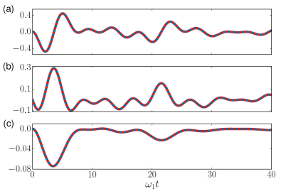
Figure S1: In all cases the parameters are fixed to $N=4$, $\delta=0.25\omega_{1}$, $\lambda=0.3\omega_{1}$ and $\gamma_{j}/\omega_{j}=0.05$. Red solid lines correspond to exact numerical results, blue dashed lines to the analytical expressions derived in this section. (a) $\langle\hat{\sigma}^{x}_{1}(t)\rangle$, considering the initial condition $|\Psi_{0}\rangle=(|0\rangle+|F_{2}\rangle)/\sqrt{2}$. (b) Imaginary part of $\langle\hat{\sigma}^{-}_{1}(t)\hat{\sigma}^{+}_{2}(0)\rangle$. Notice that the real part of this quantity is the same as (a). (c) $\langle\hat{\sigma}^{x}_{1}(t)\hat{\sigma}^{x}_{2}(t)\rangle$, considering the initial condition $|\Psi_{0}\rangle=(|0\rangle+|F_{2}\rangle)/\sqrt{2}$.

S4 Additional results about synchronization

We present further results that complement the discussion on the emergence of synchronization of the main text. In particular we show an example of a synchronized trajectory for region I and II S4.1, we give more details on the effect of varying spin’s dissipation strength S4.2, and on varying the size of the chain S4.3, and we show how the two-time correlation functions change with detuning and coupling S4.4.

S4.1 Synchronized trajectories

In Fig. S2 we show two examples of synchronized trajectories. In (a) we plot a case in region II, while in (b) a case in region I. We only show two spin’s coherences, $\langle\sigma^{x}_{1}\rangle$ and $\langle\sigma^{x}_{2}\rangle$, for clarity, although all of them are synchronized. In both cases we can see that after a transient, the spins synchronize almost in anti-phase and at the slow frequency, corresponding to the eigenmode with smallest decay rate.

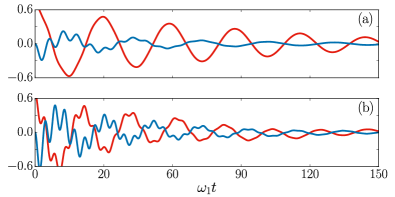
Figure S2: Synchronized trajectories for spins $\langle\sigma_{2}^{x}\rangle$ (red) and $\langle\sigma_{3}^{x}\rangle$ (blue), with initial condition $|\Psi(t=0)\rangle=|0\rangle/\sqrt{2}+(|\{1\}_{2}\rangle+\{1\}_{4})/2$. In (a) we fix $\lambda=0.1\omega_{1}$, $\delta=0.75\omega_{1}$ (SS II), while in (b) $\lambda=0.475\omega_{1}$, $\delta=0.85\omega_{1}$ (SS I). In both cases we have $N=4$ and $\gamma_{j}=0.05\omega_{j}$.

S4.2 Synchronization maps for various dissipation strengths

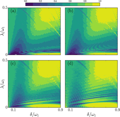
Figure S3: Map of SS among all spin pairs $\mathcal{C}_{T}(t)=\prod_{i<j}\mathcal{C}_{\langle\hat{\sigma}^{x}_{i}\rangle,\langle\hat{\sigma}^{x}_{j}\rangle}(t)$ at $\gamma_{1}t=10$ and $\omega_{1}\Delta t=80$, varying detuning and coupling strength, and with $|\Psi(t=0)\rangle=|0\rangle/\sqrt{2}+(|\{1\}_{2}\rangle+|\{1\}_{3}\rangle)/2$. Strong SS is found at the yellow (light color) regions I (intra-band synchronization) II (inter-band synchronization) ($\mathcal{C}_{T}\geq 0.9$). For all figures $\omega_{1}=1$, while in (a) $\gamma_{j}/\omega_{j}=0.005$, in (b) $\gamma_{j}/\omega_{j}=0.01$, in (c) $\gamma_{j}/\omega_{j}=0.025$ and in (d) $\gamma_{j}/\omega_{j}=0.05$. (d) corresponds to Fig. 2(a) of the main text, and we have included it to ease comparison.

In this section we analyze the effects of varying $\gamma_{j}/\omega_{j}$ over the emergence of spontaneous synchronization (SS) for all the considered parameter region (Fig. 2(a) main text). In Fig. S3 we plot the synchronization map for increasing values of the ratio $\gamma_{j}/\omega_{j}$, (a)-(d), from $0.005$ to $0.05$ respectively. Comparing these plots, we observe that the main difference is the change in size of region II of synchronization (small $\lambda$ and large $\delta$), which diminishes with the ratio $\gamma_{j}/\omega_{j}$. Indeed, the value of $\lambda$ above which SS II is no longer found diminishes strongly, while the range of $\delta$ for which there is SS does not change significantly. Conversely, the other regions of the map do not change significantly when varying the dissipation strength. The decreasing size of region II is explained by recalling the mechanism behind SS in this region. As we explain in the main text, SS in region II emerges because the small difference between the eigenfrequencies ($\nu_{l}$’s) of the same band is blurred by the decay rates ($\Gamma_{l}$’s), resulting in an effective two body behavior (Fig. 3(d) main text). When decreasing $\gamma_{j}/\omega_{j}$, the $\Gamma_{l}$’s become smaller relative to the $\nu_{l}$’s, and the dynamics of the system resolves better small frequency differences. This implies that the effective two-body behavior will be lost for smaller values of $\lambda$, hence hindering SS.

S4.3 Synchronization in larger chains

Figure S4: Synchronization map as product of Pearson correlation between spin pairs coherence operators $\mathcal{C}_{T}(t)=\prod_{i<j}\mathcal{C}_{\langle\hat{\sigma}^{x}_{i}\rangle,\langle\hat{\sigma}^{x}_{j}\rangle}(t)$ at $\gamma_{1}t=10$ and $\omega_{1}\Delta t=80$, varying detuning and coupling strength, and with $|\Psi(t=0)\rangle=|0\rangle/\sqrt{2}+\sum_{j=1}^{N}|\{1\}_{j}\rangle/\sqrt{2N}$. Strong SS is found at the yellow regions ($\mathcal{C}_{T}\geq 0.9$). (a) For a chain of $N=6$ spins. (b) For a chain of $N=8$ spins. For both figures $\gamma_{j}=0.05\omega_{j}$.

In this section we present the synchronization maps for larger chains of $N=6$ and $N=8$. Comparing figure S4 (a) and (b) with Figure 2(a) of the main text, we observe how synchronization in region I rapidly disappears as the size of the chain is increased. This is due to the fact that it depends on the difference between eigenvalues of the same band, which tends to vanish for increasing size $N$. In contrast synchronization of region II is rather robust as it depends on the fixed gap $\delta$.

S4.4 Two-time correlation functions in synchronized and unsynchronized regions

In Fig. S5 we plot several examples of the two-time correlation given in (S35) for $j=1$ and $j^{\prime}=2$. In (a) we plot examples for weak coupling ($\lambda=0.05\omega_{1}$), in (c) for strong coupling ($\lambda=0.5\omega_{1}$) and in (b) for a coupling strength in which there is no synchronization ($\lambda=0.2\omega_{1}$). We plot in different colors three different detunings: $\delta=0.3\omega_{1}$ (gold), $\delta=0.5\omega_{1}$ (blue), $\delta=0.8\omega_{1}$ (red). In Fig. S5a there are effectively only two peaks, and we can appreciate how when increasing the detuning one of the peaks becomes significantly thinner, indicating SS of region II. In contrast, if we increase the coupling to $\lambda=0.2\omega_{1}$, four different peaks emerge (Fig. S5b). In this case there are two peaks which become thiner as detuning is increased, however both of them display a similar width, hindering SS. In contrast, for stronger coupling (Fig. S5c), these two peaks display clearly different widths. This asymmetry in the decay rates of the eigenmodes is what enables synchronization in region I.

We finally mention that this kind of two-time correlations has also proven useful in the study of stationary synchronization, reported in Ref. S_SyncAtomicEnsemb for two detuned and optically pumped clouds of atoms. Stationary SS arises for certain parameters and is characterized by the presence of only one frequency, i.e. the presence of a single peak. Thus, transient SS response to fluctuations or to preparation in an out of equilibrium state are oscillations at multiple frequencies at first, but at just one frequency after a transient while in the pumped system S_SyncAtomicEnsemb oscillations occur at a single frequency. The illuminating quantity is the two-time correlation spectrum as it provides a full characterization of the frequencies of the system. This quantifies not only stationary SS S_SyncAtomicEnsemb (leading to a single peak) but can also signal the presence of multiple dissipative time scales, crucial for the presence of transient synchronization.

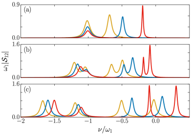
Figure S5: $\omega_{1}|\mathcal{S}_{12}(\nu/\omega_{1})|$ for different couplings and detunings. In (a) $\lambda=0.05\omega_{1}$, in (b) $\lambda=0.2\omega_{1}$, and in (c) $\lambda=0.5\omega_{1}$. Different line colors correspond to different detunings: gold $\delta=0.3\omega_{1}$, blue $\delta=0.5\omega_{1}$, red $\delta=0.8\omega_{1}$. In all cases $N=4$ and $\gamma_{j}=0.05\omega_{j}$.

References

- (1) A. Pikovsky, M. Rosenblum, and J. Kurths, Synchronization: A Universal Concept in Nonlinear Sciences, Cambride Nonlinear Science Series (Cambridge University Press, Cambridge, 2003).
- (2) F. Galve, G L. Giorgi, and R. Zambrini, in Lectures on General Quantum Correlations and their Applications (Eds.: F. Fanchini, D. Soares Pinto, G. Adesso), Springer, Cham, CH 2017, pp. 393-420.
- (3) P. P. Orth, D. Roosen, W. Hofstetter, and K. Le Hur, Phys. Rev. B 82, 144423 (2010).
- (4) G. L. Giorgi, F. Galve, G. Manzano, P. Colet, and R. Zambrini, Phys. Rev. A 85, 052101 (2012); G. Manzano, F. Galve, and R. Zambrini, ibid. 87, 032114 (2013); C. Benedetti, F. Galve, A. Mandarino, M. G. A. Paris, and R. Zambrini, Phys. Rev. A 94, 052118 (2016).
- (5) G. L. Giorgi, F. Plastina, G. Francica, and R. Zambrini, Phys. Rev. A 88, 042115 (2013).
- (6) G. L. Giorgi, F. Galve, and R. Zambrini, Phys. Rev. A 94, 052121 (2016).
- (7) A. Cabot, F. Galve, V. M. Eguíluz, K. Klemm, S. Maniscalco, and R. Zambrini, npj Quantum Inf. 4, 57 (2018).
- (8) H. Eneriz, D. Z. Rossatto, M. Sanz, E. Solano, arXiv:1705.04614 (2017).
- (9) G. Manzano, F. Galve, G. L. Giorgi, E. Hernandez-Garcia, and R. Zambrini, Sci. Rep. 3, 1439 (2013).
- (10) B. Bellomo, G. L. Giorgi, G. M. Palma, and R. Zambrini, Phys. Rev. A 95, 043807 (2017).
- (11) M. R. Hush, W. Li, S. Genway, I. Lesanovsky, and A. D. Armour, Phys. Rev. A 91 061401(R) (2015).
- (12) A. Mari, A. Farace, N. Didier, V. Giovannetti, and R. Fazio, Phys. Rev. Lett. 111, 103605 (2013)
- (13) T. E. Lee and H. R. Sadeghpour, Phys. Rev. Lett. 111, 234101 (2013).
- (14) T.E. Lee, C.-K. Chan, and S. Wang, Phys. Rev. E 89, 022913.
- (15) S. Walter, A. Nunnenkamp, and C. Bruder, Ann. Phys. 527, 131138 (2015).
- (16) M. Xu, D. A. Tieri, E. C. Fine, J. K. Thompson, and M. J. Holland, Phys. Rev. Lett. 113, 154101 (2014).
- (17) B. Zhu, J. Schachenmayer, M. Xu, F. Herrera, J. G. Restrepo, M. J. Holland, and A. M. Rey, New J. Phys. 17, 083063 (2015).
- (18) C. Davis-Tilley and A. D. Armour, Phys. Rev. A 94, 063819 (2016).
- (19) B. Militello, H. Nakazato, and A. Napoli, Phys. Rev. A 96, 023862 (2017).
- (20) M. Xu, S. B. Jäger, S. Schütz, J. Cooper, G. Morigi, and M. J. Holland, Phys. Rev. Lett. 116, 153002 (2016).
- (21) J. M. Weiner, K. C. Cox, J. G. Bohnet, and J. K. Thompson, Phys. Rev. A 95, 033808 (2017).
- (22) S. Boccaletti, J. Kurths, G. Osipov, D.L. Valladares, C.S. Zhou, Phys. Rep. 366, 1 (2002).
- (23) A. Arenas, A. Diaz-Guilera, J. Kurths, Y. Moreno, C. Zhou, Phys. Rep. 469, 93 (2008).
- (24) G. Heinrich, M. Ludwig, J. Qian, B. Kubala, and F. Marquardt, Phys. Rev. Lett. 107, 043603 (2011); A. Cabot, F. Galve, and R. Zambrini, New J. Phys 19, 113007 (2017).
- (25) A. Roulet and C. Bruder, Phys. Rev. Lett. 121, 053601 (2018).
- (26) J. G. Bohnet, Z. Chen, J. M. Weiner, D. Meiser, M. J. Holland, and J. K. Thompson, Nature 484, 78 (2012).
- (27) A. Shankar, J. Cooper, J. G. Bohnet, J. J. Bollinger, and M. Holland, Phys. Rev. A 95, 033423 (2017).
- (28) H. Schwager, J. I. Cirac, and G. Giedke, Phys. Rev. A 87, 022110 (2013).
- (29) C. Gross and I. Bloch, Science 357, 995 (2017).
- (30) N. Lörch, S. E. Nigg, A. Nunnenkamp, R. P. Tiwari, and C. Bruder Phys. Rev. Lett. 118, 243602 (2017).
- (31) D. Jaksch, C. Bruder, J. I. Cirac, C. W. Gardiner, and P. Zoller, Phys. Rev. Lett. 81, 3108 (1998).
- (32) D. Porras and J. I. Cirac, Phys. Rev. Lett. 92 207901 (2004); J. Simon, W. S. Bakr, R. Ma, M. Eric Tai, P. M. Preiss, and M. Greiner, Nature 472, 307 (2011); H. Labuhn, D. Barredo, S. Ravets, S. de Léséleuc, T. Macrì, T. Lahaye, and A. Browaeys, Nature 534, 667 (2016).
- (33) G. Lindblad, Commun. Math. Phys. 48, 119 (1976). V. Gorini, A. Kossakowski, and E. C. G. Sudarshan, J. Math. Phys. 17 821 (1976).
- (34) I. Marzoli, J. I. Cirac, R. Blatt, and P. Zoller, Phys. Rev. A 49, 2771 (1994).
- (35) J. I. Cirac, R. Blatt, P. Zoller, and W. D. Phillips, Phys. Rev. A 46, 2668 (1992).
- (36) J. Sebby-Strabley, M. Anderlini, P. S. Jessen, and J. V. Porto, Phys. Rev. A 73, 033605 (2006); J. Sebby-Strabley, B. L. Brown, M. Anderlini, P. J. Lee, W. D. Phillips, J. V. Porto and P. R. Johnson, Phys. Rev. Lett. 98, 200405 (2007); S. Fölling, S. Trotzky, P. Cheinet, M. Feld, R. Saers, A. Widera, T. Müller and I. Bloch, Nature 448, 1029 (2007); M. Lohse, C. Schweizer, O. Zilberberg, M. Aidelsburger and I. Bloch, Nat. Phys. 14, 3584 (2016).
- (37) See Supplemental Material (below this section) for details on the derivation of the results presented in the main text, which includes Refs. Cohen ; Jaksch2 ; Spins2 ; Spins3 ; Spins4 ; cooling2 .
- (38) C. Cohen-Tannoudji et al, Atom-Photon Interactions (New York: Wiley, 1992) pp 38-48.
- (39) D. Jaksch and P. Zoller, Ann. Phys. 315, 52 (2005).
- (40) L.-M. Duan, E. Demler, and M. D. Lukin, Phys. Rev. Lett. 91, 090402 (2003).
- (41) J. J. García-Ripoll, and J. I. Cirac, New J. Phys. 5, 76 (2003).
- (42) A. Imambekov, M. Lukin, and E. Demler, Phys. Rev. A 68, 063602 (2003).
- (43) R. Taieb, R. Dum, J. I. Cirac, P. Marte, and P. Zoller, Phys. Rev. A 49, 4876 (1994).
- (44) J. M. Torres, Phys. Rev. A 89, 052133 (2014).
- (45) The eigenfrequencies (decay rates) given by (S19), are denoted by () with . The first elements correspond to the band ’’ with the , while the next to the band ’’ with .
- (46) M. Gross and S. Haroche, Phys. Rep. 93, 301 (1982).
- (47) J. Gambetta, A. Blais, D. I. Schuster, A. Wallraff, L. Frunzio, J. Majer, M. H. Devoret, S. M. Girvin, and R. J. Schoelkopf, Phys. Rev. A 74, 042318 (2006).
- (48) H. J. Carmichael, Statistical Methods in Quantum Optics 1: Master Equations and Fokker-Planck Equations (Theoretical and Mathematical Physics) (Springer, Berlin, 1998) pp 19-28.

References

- (1) C. Cohen-Tannoudji et al, Atom-Photon Interactions (New York: Wiley, 1992) pp 38-48.
- (2) D. Jaksch, C. Bruder, J. I. Cirac, C. W. Gardiner, and P. Zoller, Phys. Rev. Lett. 81, 3108 (1998).
- (3) D. Jaksch and P. Zoller, Ann. Phys. 315, 52 (2005).
- (4) H. Schwager, J. I. Cirac, and G. Giedke, Phys. Rev. A 87, 022110 (2013).
- (5) L.-M. Duan, E. Demler, and M. D. Lukin, Phys. Rev. Lett. 91, 090402 (2003).
- (6) J. J. García-Ripoll, and J. I. Cirac, New J. Phys. 5, 76 (2003).
- (7) A. Imambekov, M. Lukin, and E. Demler, Phys. Rev. A 68, 063602 (2003).
- (8) J. I. Cirac, R. Blatt, P. Zoller, and W. D. Philips, Phys. Rev. A 43, 2668 (1992).
- (9) R. Taieb, R. Dum, J. I. Cirac, P. Marte, and P. Zoller, Phys. Rev. A 49, 4876 (1994).
- (10) I. Marzoli, J. I. Cirac, R. Blatt, and P. Zoller, Phys. Rev. A 49, 2771 (1994).
- (11) J. M. Torres, Phys. Rev. A 89, 052133 (2014).
- (12) B. Bellomo, G. L. Giorgi, G. M. Palma, and R. Zambrini, Phys. Rev. A 95, 043807 (2017).
- (13) H. J. Carmichael, Statistical Methods in Quantum Optics 1: Master Equations and Fokker-Planck Equations (Theoretical and Mathematical Physics) (Springer, Berlin, 1998) pp 19-28.
- (14) M. Xu, D. A. Tieri, E. C. Fine, J. K. Thompson, and M. J. Holland, Phys. Rev. Lett. 113, 154101 (2014).