The Marginal Stability of the Metastable TAP States.

Abstract

The existing investigations on the complexity are extended. In addition to the Edward-Anderson Parameter $q_{2}$ the fourth moment $q_{4}=1/N\sum_{i}m_{i}^{4}$ of the magnetizations $m_{i}$ is included to the set of constrained variables and the constrained complexity $\Sigma(T;q_{2},q_{4})$ is numerical determined. The maximum of $\Sigma(T;q_{2},q_{4})$ (representing the total complexity) sticks at the boundary for temperatures at and below a new critical temperature. This implies marginal stability for the nearly all metastable states. The temperature dependence of the lowest value of the Gibbs potential consistent with various physical requirements is presented.

I Introduction

The Thouless-Anderson-Palmer (TAP) approach tap ; tp ; tt to the Sherrington and Kirkpatrick (SK) model sk plays a central role in the attempt to understand the physics of spin glasses and related interdisciplinary problems (neural networks, computer science, theoretical biology, econophysics etc.). The system exhibits meta-stability below the spin glass temperature.

The well established work of Bray and Moore (BM) bm leads to a finite complexity below the spin glass temperature, which implies an exponential increase of the number of metastable TAP states with increasing system size. It is essential to count exclusively the physical states and neglect non-physical ones. However, the BM and subsequent work CGPM ; abm ; muller do not completely satisfy this requirement.

An alternative method to work out the characteristic properties of the metastable TAP states are numerical investigations BM79 ; mod2 ; p03 ; abm ; am19 based on iteration techniques or phenomenological dynamics for systems of finite size. The numerical determined fix-points are interpreted as metastable TAP states. Extrapolation to infinite size systems results in the conclusion that these states are marginally stable. Such an extrapolation procedure, however, leads generally to some uncertainty. Note in this context, that the numerical investigation are usually performed for systems with just some hundreds spins. Increasing the system size results in a drastic reduce of the rate finding a TAP state.

In this work the existing approaches on the complexity are extended by the additional inclusion of the forth moment of the magnetizations to the set of constrained variables. This procedure enables a complete counting of the physical TAP states. In section II the results of the calculation are presented. The total complexity and various averages are discussed to some detail in section III. Finally conclusions are drawn in section IV.

II calculation

More than four decades ago SK introduced the spin glass Hamiltonian

$$H=-\frac{1}{2}\sum_{i\neq j}J_{ij}S_{i}S_{j}$$

of $N$ Ising spins ($S_{i}=\pm 1)$. The bonds $J_{ij}$ are independent random variables with zero means and standard deviations $N^{-1/2}$ (which fixes the spin glass temperature to $T_{sg}=1$). According to the TAP approach tap ; tp ; tt the energy

$$U=N(w-\frac{1}{2T}(1-q_{2})^{2})\quad,\quad w=-\frac{1}{2N}\sum_{i\neq j}J_{ij}m_{i}m_{j}\;,$$ (1)

the entropy

$$S=\sum_{i}s_{0}(m_{i})-\frac{N}{4T^{2}}(1-q_{2})^{2}\quad,\quad s_{0}(m)=-\frac{1+m}{2}\ln\frac{1+m}{2}-\frac{1-m}{2}\ln\frac{1-m}{2}$$ (2)

and consequently the Gibbs potential $G(T,m_{i})=U-TS$ are given in terms of the local magnetizations $m_{i}$ and the temperature $T$ , where $q_{k}$ is defined as

$$q_{k}=N^{-1}\sum_{i}m_{i}^{k}\quad(k=2,4).$$ (3)

In general the local magnetic fields $h_{i}$ are determined by the TAP equations $h_{i}=\partial G/\partial m_{i}$. This work is exclusively restricted to the case $h_{i}=0$ and the TAP equations reduce to

$$G_{i}\equiv\frac{T}{2}\ln\frac{1+m_{i}}{1-m_{i}}-\sum_{j}J_{ij}m_{j}+\frac{1}{T}(1-q_{2})m_{i}=0\quad,$$ (4)

where the definition $G_{i}$ is introduced for later use. As shown by the present author tp the $m_{i}$ have to satisfy the two convergence criteria

$$c_{1}\equiv T^{2}-1+2q_{2}-q_{4}>0\,\quad,\quad c_{2}\equiv T^{2}-2q_{2}+2q_{4}>0\quad.$$ (5)

Criterion $c_{1}$ is generally accepted and is related to the de Almeida Thouless condition at for the SK solution. Criterion $c_{2}$ is controversial owen ; abm .

These criteria are of some importance for the present work. They result from an application of a theorem of Pastur pastur , which requires the in-dependency of the variables $m_{i}$ from the bonds $J_{ij}$. For a Gibbs potential, indeed these magnetizations $m_{i}$ are the free and independent variables. Note, that for every thermodynamic stability analysis one has to study the influence of all possible $m_{i}$ values including the $J_{ij}$ independent values. This requirement is also essential for the integration procedure used in this work. Thus the application of the theorem of Pastur is justified (Comparenote1 ) and $c_{2}>0$ is a necessary (but probably not sufficient ni ) convergence condition for the expansion tp .

Further support for validity of both criteria result from the fact, that they are necessary to prove the positivity of the entropy $S(T,{m_{i}})$ t00 . Simple examples leading to a negative entropy, if $c_{2}<0$ , can easily be constructed (see beispiel .) Consequences of the criteria (5) to the $T$-dependence of $q_{2}$ and $q_{4}$ has already been presented in t0 .

The present approach is related to the studies bm ; CGPM ; abm of the complexity

$$\Sigma(T,\Omega)=N^{-1}\log{\cal N}(T,\Omega)$$ (6)

which describes the extensive number ${\cal N}$ of solutions of TAP equations (4)

$${\cal N}(T,\Omega)=\int_{-1}^{1}\prod_{i}dm_{i}\;\delta(G_{i})\;{\cal C}(\Omega)\;|\det\partial G_{l}/\partial m_{k}|\,,$$ (7)

where $G_{i}$ is defined in Eq.(4). Constraints are considered in the term ${\cal C}(\Omega)$, which is chosen in this work as

$${\cal C}=\delta(q_{2}-\frac{1}{N}\sum_{i}m^{2}_{i})\;\delta(q_{4}-\frac{1}{N}\sum_{i}m^{4}_{i})\,\delta(w-\frac{1}{2N}\sum_{ij}m_{i}J_{ij}m_{j})$$ (8)

and the set of constrained variables is $\Omega=\{q_{2},q_{4},w\}$. The inclusion of $q_{4}$ is new, but is essential to take into account the restrictions due to criteria (5). Note that $q_{4}$ is a sum of single particle terms and the modifications due to such terms are simple. The use of $w$ instead of the Gibbs potential is technical and simplifies the calculation.

Following the previous work bm ; CGPM ; abm and adopting the notation of CGPM the calculation of the complexity leads to

$$\Sigma(T,\Omega)=\Sigma_{0}+\log\int dm\ e^{{\cal L}(\Omega,m)}\,$$ (9)

where

$$\Sigma_{0}=-\lambda q_{2}-\mu q_{4}-\Delta(1-q_{2})-\frac{\Delta^{2}}{2\beta^{2}}\;-\frac{1}{2}\log(2\pi\beta^{2}q_{2})+\frac{\beta^{2}v^{2}q_{2}^{2}}{4}$$ (10)

and

$${\cal L}(\Omega,m)=\lambda m^{2}+\mu m^{4}-\frac{[\tanh^{-1}(m)-\Delta m]^{2}}{2\beta^{2}q_{2}}-\log(1-m^{2})$$ (11)

with $\beta=1/T$. The variables $\lambda,\Delta,\mu,v$ enter via the Fourier representations of the $\delta$-functions in the calculation. In the limit $N->\infty$ steepest decent methods are applied. The stationary of $\Sigma(T,\Omega)$ with respect to $\lambda,\Delta,\mu,v$ leads to

$$q_{2} = \langle\langle m^{2}\rangle\rangle$$ (12)

$$\beta w = -\frac{\beta^{2}}{2}vq_{2}^{2}-q_{2}\Delta-\beta^{2}q_{2}(1-q_{2})$$ (13)

$$\Delta = -\frac{\beta^{2}}{2}(1-q_{2})+\frac{1}{2q_{2}}\langle\langle m\tanh^{-1}\,(m)\rangle\rangle-\frac{\beta^{2}}{2}vq_{2}$$ (14)

$$q_{4} = \langle\langle m^{4}\rangle\rangle$$ (15)

with

$$\langle\langle F(m)\rangle\rangle=\ \frac{1}{\int dm\ e^{{\cal L}(\Omega,m)}}\ \int dm\ F(m)\ e^{{\cal L}(\Omega,m)}.$$ (16)

The set of Eqs.(9-14) correspond to the Eqs.(56-61) of CGPM with the replacements $f\rightarrow w,\phi_{0}\rightarrow 0,\,u\rightarrow v,q\rightarrow q_{2},B\rightarrow 0$ and the additional terms proportional to $\mu$ resulting from the inclusion of $q_{4}$. The apparent differences of Eq.(10) and Eq.(56) of CGPM result from a simplification using Eq.(13). Setting $B=0$ corresponds to an exclusion of a non-physical solution. Eq.(15) is obvious and results from the stationary with respect to $\mu$. For more details of the calculation and for the performed approximations it is referred to the previous work bm ; CGPM ; abm .

Note, however, that as long as $q_{2}$ and $q_{4}$ satisfy the criteria (5) the value of the determinant $\det\partial G_{k}/\partial m_{l}$ in Eq.(7) is always positive. All previous work disregards the modulus with not completely satisfying arguments.

III applications

A. Total complexity

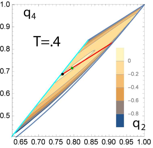
Figure 1: Contour-plot of the complexity $\Sigma(T;q_{2},q_{4},v=0)$ at $T=.4\;$: The cyan and the red boundaries represent the lines $c_{1}=0$ and $c_{2}=0$. The region above the red line is the relevant area with $c_{2}>0$. The maximum value represents the total complexity $\Sigma_{tot}(T=.4)$ and its position is indicated by the green dot. The black dot indicates the position of $g_{0}$.

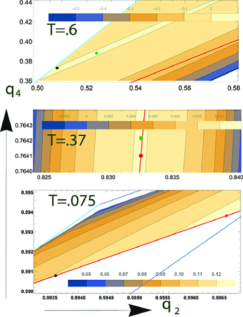
Figure 2: Contour-plot of the complexity $\Sigma(T;q_{2},q_{4},v=0)$ far above, near and far below the critical temperature $T_{1}=.367$: Red Dots mark boundary maxima and green dots denote maxima in the interior compatible with both criteria (5). Black dots indicate the position of $g_{0}$

As first application the BM work bm for the total complexity $\Sigma_{tot}(T)$ is reanalysed, which describes the total number of TAP states.

Setting $v=0$ in Eqs.(9-15) the resulting equations determine the complexity $\Sigma(T;q_{2},q_{4},v=0)$ for fixed values of $q_{2}$ and $q_{4}$ . These equations are numerical investigated for all possible values of $q_{2},q_{4}$ and for all temperatures $T<1$.

As example $\Sigma(T=.4;q_{2},q_{4},v=0)$ is plotted in the $q_{2}-q_{4}$ plane in FIG.1 . The region of allowed $q_{2}-q_{4}$ values is restricted by $q_{2}^{2}\leq q_{4}\leq q_{2}$ and by the criteria (5). The cyan and the red boundaries represent the lines $c_{1}=0$ and $c_{2}=0$, respectively. The physical relevant region $c_{2}>0$ is above the red borderline. The region below the red line with $c_{2}<0$ has no physical significance.

The absolute maximum of $\Sigma(T;q_{2},q_{4},v=0)$ in the $q_{2}-q_{4}$ plane represents $\Sigma_{tot}(T)$ and can generally be located in the interior or on the boundary of the relevant region. For temperatures $T\geq T_{1}$ the maximum is within the region and for $T\leq T_{1}$ the maximum is located on the boundary $c_{2}=0$. The numerical value of the critical temperature $T_{1}$ is given by

$$T_{1}=.367\quad.$$ (17)

The coordinates of the maxima are determined by $\mu=0$ and by $\partial\Sigma/\partial q_{2}=0$ or by $c_{2}=0$. At $T_{1}$ the internal maximum coincides with the boundary maximum.

In addition to FIG.1, which gives an overview, some details are presented in FIG.2 for $T=.6$ , for $T=.37$ and for $T=.075$. The internal maxima and the boundary maxima are marked by a green and red dots, respectively. (On the scale of FIG. 1 these two minima are not separated.)

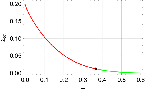
Figure 3: Total complexity $\Sigma_{tot}(T)$ versus temperature $T$ : The red branch result from maxima on the boundary ($T<T_{1}$) and the green branch result from internal maxima ($T>T_{1}$). The black dot marks the critical point $T_{1}$. (For $T>.6$ the approximative expansion of bm is very accurate.)

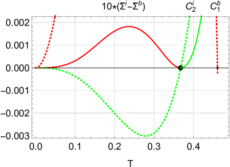
Figure 4: Separation of the extrema : Plotted is the difference of the internal maximum $\Sigma^{i}$ to the boundary maximum $\Sigma^{b}$ (red and green full lines). The corresponding criteria $c_{2}^{i}$ and $c_{1}^{b}$ are represented by dotted red and green lines. The black dot marks the critical temperature $T_{1}$.

$\Sigma_{tot}(T)$ has two branches $\Sigma^{i}$ and $\Sigma^{b}$ resulting from the two different maxima. $\Sigma^{i}$ is identical to BM and represents the stable branch for $T>T_{1}$. The quantity characteristic for the transition is $c^{i}_{2}$, the $c_{2}$ for the internal maximum, which tends to zero for $T\rightarrow T_{1}$ from above. Below $T_{1}$ criterion $c^{i}_{2}$ is negative, the border maximum is the physical one and the the branch $\Sigma^{b}$ with $c^{b}_{2}=0$ is relevant. FIG.3 shows the $T$ dependence of these two branches. Both have continuations from $T_{1}$ to the irrelevant temperatures regions. The difference of their extremal values is small (in the order of $10^{-4}$ ) and are plotted in FIG.4.

The presented results are new and have the important consequence that nearly all TAP solutions are marginal stable for temperatures at and below $T_{1}$. Previous claims of marginality muller ; BM79 ; mod2 ; p03 ; abm ; am19 are exclusively based on $c_{1}=0$ and differ therefore from the present findings, which are based on $c_{2}=0$. Note in addition, that the classical BM work on the total complexity does not include any marginality for any temperature below T=1.

B. Averages

Next some physical interesting averages for the Gibbs potential $g$ and the energy $u$ per spin are calculated. According to Eqs.(1) and (2) these averages are given by

$$g=w-\frac{\beta}{4}(1-q_{2})^{2}-T\langle\langle s_{0}(m)\rangle\rangle$$ (18)

and by

$$u=w-\frac{\beta}{2}(1-q_{2})^{2}\quad.$$ (19)

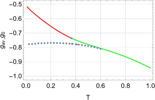
Figure 5: Gibbs potential: $T$-dependence of $g_{av}$ (full lines) and $g_{0}$ (dots).

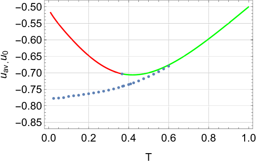
Figure 6: Energy: $T$-dependence of $u_{av}$ (full lines) and $u_{0}$ (dots).

Let us first consider the averages over all TAP states with equal weights. These ’white’ averages $g_{av}$ and of $u_{av}$ are determined by the extremal values of the parameters of the total complexity $\Sigma_{tot}(T)$. The temperature dependence for $T\leq 1$ of $g_{av}$ and of $u_{av}$ is plotted in FIG.5 and in FIG.6, respectively. The strange increase of $u_{av}$ with decreasing $T$ results from the fast increasing number of TAP solutions with high energies. These white averages have therefore no physical significance or any relevance for low temperatures.

There is an interesting, alternative averaging, that leads to the lowest value $g_{0}$ of the Gibbs potential consistent with both, the existence condition of TAP solutions $\Sigma\geq 0$ and the validity of the criteria(5). To attack this problem the complete set of Eqs.(9-15,18,19) is needed. Keeping $q_{2},q_{4}$ and $v$ constant the parameters $\lambda,\Delta,$ and $\mu$ are determined numerically with Eqs.(12,14,15). Repeating this procedure for all possible values of $q_{2},q_{4}$ and $v$ the dependence of the complexity $\Sigma$ , of $w$ and of the Gibbs potential $g$ on these quantities is obtained according to Eqs.(10,13,18). Finally the minimum $g_{0}$ of the Gibbs potential is determined in the region of the allowed values of $q_{2}$ , $q_{4}$ and $\Sigma$. The findings are a vanishing complexity $\Sigma=0$ for all temperatures, which ensures at least the presence of one TAP state in the thermodynamic limit $N\rightarrow\infty$.

The resulting $g_{0}$ and the corresponding energy $u_{0}$ are plotted in FIG.5 and in FIG.6, respectively. Both quantities exhibits the expected temperature dependence and are similar to the results of the replica approach andrea . This is remarkable as both approaches use different averages. A second interesting point is the fact that the location of $g_{0}$ is again on the boundary $c_{2}=0$ for $T<T_{1}$ . (Compare FIG.2.)

C. Postulated marginality

Previous numerical investigations BM79 ; mod2 ; p03 ; abm ; am19 claim marginal metastable states based on $c_{1}\rightarrow 0$ in the thermodynamic limit. Therefore $c_{1}=0$ is postulated a priory in this subsection and the resulting consequences for the present approach are worked out.

The first quantity of interest is the complexity $\Sigma_{m}$, which determines the total number of TAP states with the constraint $c_{1}=0$ . This complexity $\Sigma_{m}$ is given by the absolute maximum of $\Sigma(T;q_{2},q_{4}=2q_{2}-1+T^{2},v=0)$ , as function of $q_{2}.$ Again two temperature regimes exist, which are separated by a critical temperature $T_{av}^{m}=.459$ . For $T>T_{av}^{m}$ the maximum is located within the allowed $q_{2}$ - interval $(1-1.5\;T^{2})<q_{2}<1$ and for $T\leq T_{av}^{m}$ the maximum sticks at the endpoint $q_{2}=(1-1.5\;T^{2})$ . The numerical results for $\Sigma_{m}$ are consistent to $0\leq\Sigma_{m}\leq\Sigma_{tot}$ for all temperatures, which ensures the existence of at least one TAP state with the postulated marginality. Note that this last conclusion is a priory not obvious. FIG.7 shows the temperature dependence of $\Sigma_{m}$ for $T<.6$ .

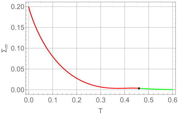
Figure 7: Complexity $\Sigma_{m}$ versus temperature $T$ : The red branch result from maxima on the boundary ($T<T_{av}^{m}$) and the green branch result from internal maxima ($T>T_{av}^{m}$). The black dot marks the critical temperature $T_{av}^{m}$.

Analogue to subsection B. the set of extremal parameters of the maximum determine the averages performed with all TAP states satisfying $c_{1}=0$. Together with Eqs.(18) and (19) this leads directly to the averages of the Gibbs potential $g_{av}^{m}$ and the energy $u_{av}^{m}$ performed with these states . Both quantities $g_{av}^{m}$ and $u_{av}^{m}$ are plotted in FIG.8. The results $g_{av}^{m}$ and $u_{av}^{m}$ are not very useful for low temperatures similar to the above findings for $g_{av}$ and $u_{av}$.

The lowest value of the Gibbs potential $g_{0}^{m}$ consistent with $c_{1}=0\;,\;c_{2}\geq 0$ and $\Sigma\geq 0$ is again determined analogue to procedure of subsection B. As before a vanishing complexity and two temperature regions are found with a sticking below a different critical temperature $T_{0}^{m}=.417$. The temperature dependence of $g_{0}^{m}$ together with the corresponding energy $u_{0}^{m}$ is plotted in FIG.8.

For $T=.2$ the numerical value is for the Gibbs potential is $g_{0}^{m}=-.7644$. This value is in remarkable agreement with the value of $\hat{g}_{0}^{m}=-.07619$ found by the dynamical investigation p03 with $c_{1}->0$ and with a vanishing complexity. The result $\hat{g}_{0}^{m}$ is added to FIG.8 as Point $C$ together with the Points $A$ and $B$ found by further investigations abm ; am19 . Even though $c_{1}->0$ is satisfied no results for the complexity are available for the points $A$ and $B$. Nevertheless these results are compatible with the present work.

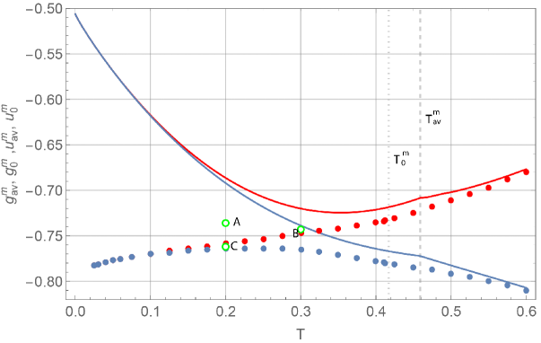
Figure 8: Gibbs Potential and Energy: $T$-dependence of $g_{av}^{m}$ (full, blue line), $u_{av}^{m}$ (full, red line), $g_{0}^{m}$ (blue dots) and $u_{0}^{m}$ (red dots). The green points A, B and C represent published values of the Gibbs potential according to abm , to am19 and to p03 , respectively.

IV Conclusion

The presented investigation of the complexity is based the inclusion of $q_{4}$ to the set of constrained variables. This extension together with a strict regard of the validity criteria for the TAP equations leads to new results in low temperatures regime. Numerically the differences to the existing approaches are rather small, the interpretations and conclusions, however, differ considerably. At and below a critical temperature $T_{1}$ nearly all TAP states are marginal stable with $c_{2}=0$, a property not found in previous theories on the total complexity. Marginal stability implies a vanishing eigenvalue of the Hessian and the divergence of a mode of the susceptibility matrix tp . The system is critical for all temperatures below $T_{1}$ and shows critical slowing down effects.

In addition to this findings consequences for averages over all metastable TAP states and averages over states with the lowest value of the Gibbs potential have been worked out for all temperatures. Moreover the influence of a different kind of marginality $c_{1}=0$ , as found by supplementary numerical investigations BM79 ; mod2 ; p03 ; abm ; am19 , has been worked out.

- (1) D. J. Thouless, P. W. Anderson, and R. G. Palmer, Phil. Mag. 35, 593 (1977).
- (2) T. Plefka, J. Phys. A: Math. Gen., 15, 1971 (1982).
- (3) T. Plefka, EuroPhys.Lett. 58, 892 (2002).
- (4) D. Sherrington and S. Kirkpatrick, Phys. Rev. Lett. 35 1972, (1975).
- (5) A. J. Bray and M. A. Moore, J. Phys. C 13, L469 (1980).
- (6) A. Cavagna, I. Giardina, G. Parisi, and M. Mézard, J. Phys. A 36, 1175 (2003) .
- (7) T. Aspelmeier, A. J. Bray and M. A. Moore, Phys. Rev. Lett. 92 087203, (2004).
- (8) M. Müller, L. Leuzzi and A. Crisanti, Phys. Rev. B 74 134431, (2006).
- (9) A. J. Bray and M. A. Moore, J. Phys. C 12, L441 (1979).
- (10) T. Plefka, Phys. Rev. B 65, 224206 (2002).
- (11) T. Plefka, cond-mat/0310782. (2003).
- (12) T. Aspelmeier and M. A. Moore, Phys. Rev. E 100 032127, (2019).
- (13) J. R. L .de Almeida and D. J. Thouless , J. Phys. A 11, 983 (1978).
- (14) J.C. Owen, J. Phys. C 15, L1071 (1982).
- (15) L.A. Pastur, Russ. Math. Surveys 28, 1 (1974).
- (16) T. Plefka, Phys. Lett. 90 A, 262 (1982).
- (17) Owen owen investigates a different question, as he conciders , which depend on the via the TAP equations and the Pastur Theorem can not be applied. There is no disagreement to tp , which investigates the Gibbs potential with free and independent . Moreover, it is generally impossible to conclude anything on the convergence of a series from a partial re-summation, as done in owen .
- (18) N Kistler , private communication (2018).
- (19) Consider a special set with , which implies and . For condition is violated. The entropy is given by , which is negative for all temperatures smaller than .
- (20) T. Plefka, J. Phys. A 15, L251 (1982).
- (21) A. Crisanti and T. Rizzo, Phys. Rev. E 65, 046137 (2002).