Patchy particles by self-assembly of star copolymers on a spherical substrate: Thomson solutions in a geometric problem with a color constraint
	Tobias M. Hain,a,c, Gerd E. Schröder-Turk∗a,b,c and Jacob J. K. Kirkensgaard∗b
	Confinement or geometric frustration is known to alter the structure of soft matter, including copolymeric melts, and can consequently be used to tune structure and properties. Here we investigate the self-assembly of $ABC$ and $ABB$ 3-miktoarm star copolymers confined to a spherical shell using coarse-grained Dissipative Particle Dynamics simulations. In bulk and flat geometries the $ABC$ stars form hexagonal tilings, but this is topologically prohibited in a spherical geometry which normally is alleviated by forming pentagonal tiles. However, the molecular architecture of the $ABC$ stars implies an additional ’color constraint’ which only allows even tilings (where all polygons have an even number of edges) and we study the effect of these simultaneous constraints. We find that both $ABC$ and $ABB$ systems form spherical tiling patterns, the type of which depends on the radius of the spherical substrate. For small spherical substrates, all solutions correspond to patterns solving the Thomson problem of placing mobile repulsive electric charges on a sphere. In $ABC$ systems we find three coexisting, possibly different tilings, one in each color, each of them solving the Thomson problem simultaneously. For all except the smallest substrates, we find competing solutions with seemingly degenerate free energies that occur with different probabilities. Statistically, an observer who is blind to the differences between $B$ and $C$ can tell from the structure of the $A$ domains if the system is an $ABC$ or an $ABB$ star copolymer system.

1 Introduction

The self-assembly of linear diblock copolymers and their phase diagram is nowadays well understood ¹, ², ³. By contrast, the study of the phase behaviour of more complex copolymer architectures, like grafts or stars ⁴, remain incomplete, due to the larger parameter space and, hence, a larger variety of possible structures ², ³, ⁵, ⁶, ⁷. Here we consider $ABC$ 3-miktoarm star terpolymers, henceforth called $ABC$ star copolymers. These are copolymers which consist of three linear chains connected at a central grafting point ⁸, ⁹, ³, ⁴, as shown in fig. (1) or (2). These star copolymers can be synthesized so that the three arms are immiscible; herein we refer to the three polymeric species as colors: blue, yellow and red. When this immiscibility drives the moieties to micro-phase separation, the arms of equal species will agglomerate into domains, which will self-assemble into complex structures. Considerable amount of work has been put towards the investigation of one type of these structures: columnar phases whose cross-sections are planar tiling patterns ¹⁰, ¹¹, ¹², ¹³, ¹⁴, ¹⁵, ¹⁶, ¹⁷, ¹⁸, ¹⁹, ²⁰.

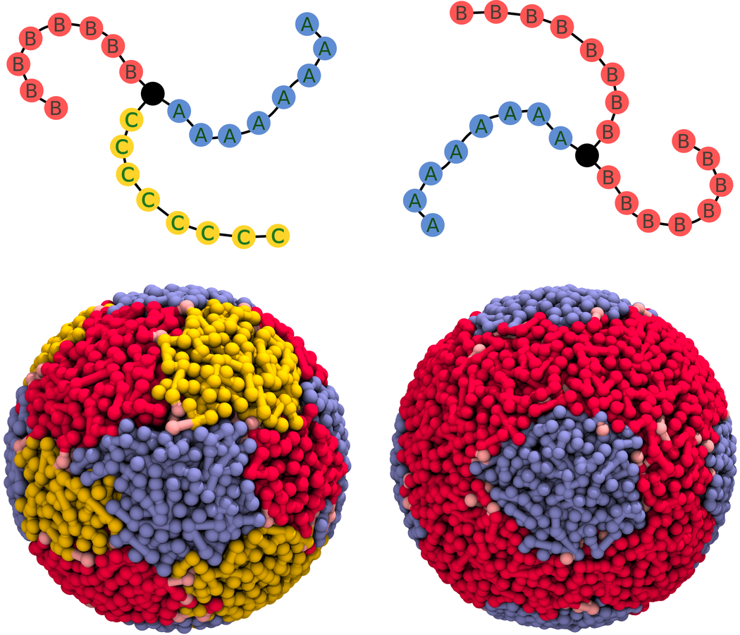
Fig.  1: Polymeric self-assembly of $ABC$ and $ABB$ star copolymers on a spherical substrate Top panel: Schematic visualization of coarse grained models of $ABC$ and $ABB$ star copolymers used for the DPD simulations. Bottom panel: Snapshots of simulations comprising $ABC$ and $ABB$ star copolymers. Polymer arms of identical color agglomerate into patches. The $ABC$ system creates a three colored tiling of the sphere, whereas the $ABB$ system builds a single tiling made up of only $A$-type patches in a $B$-type matrix.

A distinguished and important feature of $ABC$ star copolymers is that all structures arising from these molecules must be compatible with the special architecture of the latter:

1. The grafting points form triple lines¹³ where three different domains meet, which, in cross-section, corresponds to vertices of the tiling pattern.

2. Any given patch of a given color (e.g. yellow), must be surrounded by an alternating sequence of patches of the other colors (e.g. blue and red). The number of these surrounding patches must then be even ¹².

For more details see fig. (2). In this article we will refer to constraint 2 as the color-constraint.

If the star copolymers are chosen symmetrically, i.e. all arms have equal length, and with equal interaction strength between the arms, a hexagonal columnar phase is formed where a cross section perpendicular to the columns yields a planar 3-colored honeycomb pattern which we here consider as the ’ground state’ of the system. ²¹, ¹¹, ¹⁰, ¹², ¹³, ¹⁹, ¹⁶. The hexagonal tiling can be tuned into a large variety of tilings by varying the length of one of the three arms ¹⁰, ¹², ¹⁹. However, all these tilings consist of vertices of order three only, which is enforced by the molecular architecture of the star copolymers.

Apart from changing the chemical composition or interactions of the polymers, another way to tune structures is by geometric confinement. A simple analogy illustrates this fundamental geometric concept: the peel of an orange for example cannot be confined to a flat plane, without tearing or deforming it. This also applies for the star polymers: the optimal free energy configuration they form in the plane, the regular honeycomb, cannot be fitted on a spherical substrate without distorting the planar pattern.

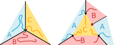
Fig.  2: Structural constraints imposed by polymer architecture: the color-constraint Left panel: Since the three different polymer arms making up domains are bonded at a central junction bead (grafting point), the latter must sit on points or lines where three different domains meet so that each arm may extend in a domain of its species. Right panel: For tiling patterns, this results in the so-called color constraint: only polygons with an even number of edges are allowed, where the types of all adjacent polygons alternate. The figure illustrates this: if a polygon with an uneven number of edges is attempted to be formed, a new interface (dashed line) and grafting point (red point) is introduced by the architecture of the stars, resulting in an even polygon.

Unlike the restriction of polymers to a thin film, the confinement to curved geometries, like spheres, does not only impose the constraint of physical confinement onto the polymers, but also introduces curvature to the system. This alters the shape and structure of the space available to the polymer melt which can enforce or prohibit some structures to form. Such curvature-related effects have been described for multiple self-assembly systems:

Several articles report on the influence of curvature on hexagonal particle orders on surfaces with positive and negative curvature, both using experiments ^{22, 23, 24, 25, 26, 27} and simulations ²⁸, ²⁹, ²⁴. Two dimensional tilings can be created from these particle assemblies by assigning each particle a polygon where the number of edges coincides with its coordination number, which is the number of neighbouring particles. While these particles would arrange in a hexagonal order in a plane, and therefore, form a perfect hexagonal tiling, defects in this patterns were found after the particles self-assembled on curved surfaces. Zhang et al. ³⁰ found similar defects in the self-assembly of $AB$ diblock copolymers confined to a spherical substrate using numerical methods to solve the Landau-Brazovskii theory. For cylinder forming diblocks, the cylinders distributed over the surface of the sphere in a generally hexagonal order, however, 5-fold defects were found. For larger systems, scars of connected 5- and 7-fold defects occur. These defects have a fundamental mathematical origin: the different topologies of the confining surface. Each tiling and polyhedra (and topological equivalents) have an intrinsic property, the Euler characteristic $\chi$, describing its topological type ³¹, ³², ³³. An Euler characteristic of $\chi=2$ corresponds to an object that is a single component without any handles or cavities, such as the sphere. A given tiling can only tessellate a surface of the same topological space, therefore surfaces having the same Euler characteristic as the tiling³². A planar, periodical hexagonal tiling has $\chi=0$, as does a torus. Therefore the hexagonal tiling can be mapped onto the latter. When a hexagonal lattice is forced onto an incompatible curved surface, as for example a sphere with $\chi=2$, the mismatch leads to ’geometric frustration’: the hexagonal lattice is incompatible with the topology of the substrate. To cope with this incompatibility defects occur in the hexagonal order.

To check if a tiling is compatible with a sphere, Euler’s formula can be used, which reads in case of a sphere³¹, ³³:

$$\chi=V-E+F=2$$ (1)

where $V$, $E$, $F$ is the number of vertices, edges and facets in the tiling. If a tiling fulfills this condition, it can be mapped onto a sphere without defects. In our case, where tilings are generated by $ABC$ star copolymers, the color constraint can be incorporated into eq. (1). Since only vertices where three edges meet are allowed, each edge is shared by two and each vertex by three facets (see also fig. 2). In this case, eq. 1 can then be expressed in terms of the number of polygons in the tiling:

$$\chi=\sum_{i}\left(\frac{i\cdot n_{i}}{3}-\frac{i\cdot n_{i}}{2}+n_{i}\right)=\sum_{i}\left(1-\frac{1}{6}i\right)n_{i}=2$$ (2)

where $n_{i}$ is the number of polygons with $i$ edges in the tiling. This equation easily shows that a hexagonal tiling is incompatible, since the term in the brackets equals zero for $i=6$. Therefore polygons with a different number of edges need to be introduced to fulfil the equation. One solution to eq. (1) for the sphere is the arrangement of 12 pentagons to an icosahedron. Since the left side of eq. (1) vanishes for hexagons, an arbitrary number of the latter can be added to the 12 pentagons and the topology will not change. A well-known configuration is the soccer ball, consisting of 12 pentagons and 20 hexagons. Apart from investigations of particles from polymer systems, abstract systems with topological defects were investigated analytically ³⁴, ³⁵, ³², ³⁶. Here the behavior of abstract disclinations from the crystalline state, for example particles with 5 neighbours in an otherwise hexagonal lattice, was investigated using free energy calculations. The results agree with the results found in the physical particle and polymer systems: the favoured state are 12 5-fold disclinations, also the above mentioned scars (connected disclinations) are found.

A very prominent problem of ordering on a sphere is the so-called Thomson problem. It was formulated by J. J. Thomson in 1904 in the context of his atomic model. The Thomson problem is the search for the minimal energy configuration of $n$ repelling electrons, all of the same negative charge $-e$, on a spherical surface³⁷. The resulting arrangement of electrons and their symmetries ³⁸, ³⁹, ⁴⁰, ⁴¹, ⁴² has been found in many seemingly unconnected problems, as for example in the design of protein virus capsides ⁴³, ⁴⁴, ⁴⁵, the construction of fullerens and nanotubes ⁴⁶, but also in more generalized Thomson problem versions ⁴⁷. To reach the minimal energy solution, the optimal coordination number of a single electron is six, however, due to the geometric frustration defects in the hexagonal order must occur, as explained above ⁴⁸. For our system, it is useful to interpret the electron positions of the Thomson problem solutions as vertices of a polyhedra. The graph of its dual polyhedron is a tiling of the sphere, where each electron is assigned a tile whose number of edges is equivalent to the coordination number of the corresponding electron. A solution of the Thomson problem, henceforth called a Thomson solutions, can therefore be described and labeled by its dual lattice, see table (1).

In conclusion, using $ABC$ star copolymers confined to a spherical shell as a model system enables the simultaneous study of two different constraints: geometric frustration and the influence of the color-constraint. To investigate the effects of each on their own, a strategy is needed to switch one of them on and off. This is accomplished by using two different kind of star molecules, the aforementioned $ABC$ stars and $ABB$ star molecules, see right panel in fig. (1). These only differ to the $ABC$ stars in that two arms are of the same species. Thus the color-constraint can be eliminated, since the grafting points of the $ABB$ stars can move freely across the interface between $A$ and $B$ type domains. The $A$ type domains, which are the tiles in the resulting tiling, can then freely move around in a $B$ type matrix.

2 Methods

2.1 Dissipative particle dynamics of star copolymers

Dissipative Particle Dynamic (DPD) simulations are used to find equilibrium configurations of the polymer systems. DPD simulations ⁴⁹, ⁵⁰ are a type of molecular dynamic simulations designed for coarse grained models of molecules, which makes it a natural fit for polymer melts ⁵¹, ⁵², ²¹, ¹¹. As all molecular dynamics simulations, the DPD method is based on the forward integration of Newton’s equation of motion in time for each particle $i$:

$$\frac{d^{2}\textbf{x}_{i}}{dt^{2}}=\frac{1}{m}\cdot\textbf{F}_{i}$$

In our case, a particle is a single bead in the polymer arms (see fig. (1)), where each bead may represent many atoms. A symmetric star copolymer then consists of a center particle with three connected arms, each consisting of a chain of bonded particles. A schematic representation of such a coarse grained polymer is shown in fig. (1).

We use the simulation package hoomd-blue ^{53, 54, 55} to perform our simulations. We will only briefly discuss the parameters used at this point, for details on the implementation we refer to ⁵⁶ and the documentation of the hoomd-blue package ⁵⁷. In this simulation package all units are given based on three reference units (distance $\mathcal{D}$, energy $\mathcal{E}$ and mass $\mathcal{M}$) which can be chosen arbitrarily. All other units, for example a force, can be derived from these units, for more details we refer to the hoomd-blue manual⁵⁷. In the course of this article, all given values are given in terms of these reference units unless stated otherwise. The package implements the DPD method following the formulation of ^{56, 50}. Here the force on particle $i$ is given as

$$\textbf{F}_{i}=\sum_{i\neq j}\left(\textbf{F}_{ij}^{\text{C}}+\textbf{F}_{ij}^{\text{D}}+\textbf{F}_{ij}^{\text{R}}\right)$$

where the sum is over all particle pairs within a cutoff radius $r_{c}=1$ around the $i$-th particle. The force consists of three contributions: a conservative force $\textbf{F}_{ij}^{\text{C}}$ representing the repulsive interactions between the particles, a dissipative force $\textbf{F}_{ij}^{\text{D}}$ and a random force $\textbf{F}_{ij}^{\text{R}}$. The latter two act as a thermostat to keep the temperature of the system constant. Since a thermostat is a built-in feature of the DPD interactions, the system is technically advanced as a $NVE$ ensemble using a standard Velocity-Verlet step algorithm, although it is effectively a $NVT$ ensemble. The conservative force is 0 only for $r_{ij}\geq r_{c}$ and is otherwise given by

$$\textbf{F}_{ij}^{\text{C}}=a_{ij}\left(1-\frac{r_{ij}}{r_{c}}\right)\hat{\textbf{r}}_{ij}$$ (3)

where $a_{ij}$ is the maximum repulsion between two particles and therefore a measure of the interactions strength, $\textbf{r}_{ij}=\textbf{r}_{i}-\textbf{r}_{j}$ and $\hat{\textbf{r}}_{ij}=\textbf{r}_{ij}/|\textbf{r}_{ij}|$. The interactions between two particles of the same species is given as $a_{ii}=75\frac{k_{\text{B}}T}{\rho}$, where $\rho$ is the number density and $k_{\text{B}}T$ the temperature in the polymer melt. The interaction parameters can be mapped onto the well established Flory-Huggins interaction parameter $\chi_{ij}$ ⁵⁸, ⁵⁹ used in polymer science using $a_{ij}=a_{ii}+3.268\chi_{ij}$ ⁶⁰. We use values of $a_{ii}=25$ and $a_{ij}=40$ that, at a temperature of $k_{B}T=1$ and a particle density of $\rho=3$, corresponds to the strong segregation limit. The single beads of the polymer chains are bonded by a harmonic potential, given as $V_{\text{H}}(r)=\frac{1}{2}k(r-r_{0})^{2}$, where $k$ measures the strength of the bond and $r_{0}$ the bond rest length. In our system we chose $k=4\,\frac{\mathcal{E}}{\mathcal{D}^{2}}$ and $r_{0}=0.88\,\mathcal{D}$ as the position of the first peak of the pair correlation function in a system of unbonded, identical particles with the given interaction parameters. Each arm in the polymers consists of 8 beads.

The confinement of the system to a spherical substrate is modelled as follows: the simulation volume is a spherical shell bounded by two repulsive spherical walls interacting with the polymers with a purely repulsive Lennard-Jones potential:

$$V_{\text{LJ}}(r)=4\epsilon\left[\left(\frac{\sigma}{r}\right)^{12}-\left(\frac{\sigma}{r}\right)^{6}\right]+\Delta V$$

where $r$ in this case is the length of the vector from the particle perpendicular to the wall, not to be confused with $r_{ij}$, the pairwise distance between two particles, see fig. (3). $\Delta V=-\left(r-r_{\text{cut}}\right)\frac{\partial V}{\partial r}\left(r_{c}\right)-V_{\text{LJ}}\left(r_{c}\right)$ and $\sigma$ is the range of the repulsive potential, $\epsilon$ would be the strength of the attractive part of the Lennard-Jones potential, however, is of no relevance in the purely repulsive version used here. While the outer wall exerts a force towards its center, the forces of the inner wall acts outwards. Hence, the wall keeps all particle inside the spherical shell they enclose. We choose $\sigma=1\mathcal{D}$ and set the cutoff of the wall potential to $r_{c}=2^{\frac{1}{6}}\sigma$ to cut the attractive tail.

The spherical walls are concentric around the origin with radii of $R_{i}=R-dR/2-\sigma$ and $R_{o}=R+dR/2+\sigma$, the shell therefore has a thickness of $dR$, as shown in fig. (3).

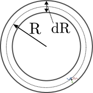
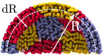
Fig.  3: Simulation setup and substrate model Left panel: Schematic sketch of a cross section of the simulation setup. The two black, bold circles represent spherical, repulsive ‘Lennard-Jones walls’ with radii of $R+\frac{dR}{2}+\sigma$ and $R-\frac{dR}{2}-\sigma$. As shown, the outer wall exerts a LJ-force on a particle along a vector perpendicular to the wall towards its center. The force of the inner shell acts outwards. Together these walls confine the polymers to a shell of thickness $dR$. Right panel: Cross section through a simulation snapshot with radius $R=8\,\mathcal{D}$ with the same quantities marked. The image shows the homogeneity of structure in the radial direction of the shell and gives an idea for the scale of the system.

The amount of curvature forced onto the system can then be tuned by varying the radius of the spherical shell. The initial position of the centers of the stars are chosen inside the simulation volume from a uniform distribution. The arms are then placed at random positions around the center. In order to achieve a well mixed configuration the system runs $5.5\times 10^{5}$ time steps where the interaction parameter between any species of particles is set to $a_{ii}=a_{ij}=25\,\frac{\mathcal{E}}{\mathcal{D}}$. After this warmup phase the parameters are set as stated above according to their species. The temperature of the system was kept constant at $k_{b}T=1$ for the entire run. All simulations have been run with time steps of $\Delta t=0.005$ and ran at least $3\times 10^{8}$ time steps, larger systems with $R>8\,\mathcal{D}$ ran $5\times 10^{8}$ time steps. After these long runs we assume that an equilibrium is reached, which is confirmed visually in random samples. The radius $R$ of the spherical shell was varied with $R=4,5,6,7,8,9,10\,\mathcal{D}$. Alternating the radius has two effects: (1) due to constant a number density of $\rho=3\,\frac{1}{\mathcal{D}^{3}}$ the number of molecules increase with a larger shell volume; (2) the curvature of the shell decreases with increasing radius. For each radius 20 configurations for each $ABC$ and $ABB$ systems were simulated with different random initialisations for statistical significance.

2.2 Structure analysis of tiling patterns

When the simulation is deemed to be equilibrated, the resulting spherical tilings are recovered from the polymer configurations using Set-Voronoi diagrams ⁶¹ as implemented in pomelo ⁶². The aim is to substitute each domain in the system with a polygon, representing a tile, where the number of edges of the latter is equal to the number of neighboring domains.

In the $ABB$ systems we characterize the structure of the A beads, considering the B particles as a matrix. We use a cluster algorithm (implemented in the trajectory analysis package freud⁶³) to identify all A domains. This provides a list of $N$ clusters, one for each $A$ type domain, each with a list of which particles it is made from. Then the Voronoi diagram of all $A$ type particles is computed, where all cells of particles belonging to the same cluster are merged, leaving one cell per cluster. The number of neighbors for each domain are determined from the number of adjacent cells sharing a common edge. The spherical tiling is recovered by representing each domain by a polygon which number of edges equals the number of neighbors.

For the visualizations of the tiling shown in fig. (4) and (6), the vertices of a tiling are placed at the grafting points where three Voronoi cells meet. The edges connecting vertices are great circle segments. Figure (4) shows a simulation snapshot on the left and a representation of the spherical tiling in the middle. We obtain 2D topological representations of the tilings through the Mercator projection as used in ³⁰. Each point on the sphere given in spherical coordinate angles $(\theta,\phi)$ with $\theta\in[-\pi/2,\pi/2]$ and $\phi\in[0,2\pi]$ is mapped in the carthesian plane by $x=R\phi$ and $y=R\ln\left(\tan\left(\frac{\pi}{4}+\frac{2}{5}\theta\right)\right)$. An example of such a projection is shown on the right hand panel of fig. (4). In these representations, the plot has periodic boundary conditions in the x direction, however, not in y direction. The top and bottom tiles therefore are not adjacent, but represent the tiles at the poles of the sphere. The purpose of the planar projections is to correctly capture the topology and neighbor relations, not the geometry, which is deformed in the projection.

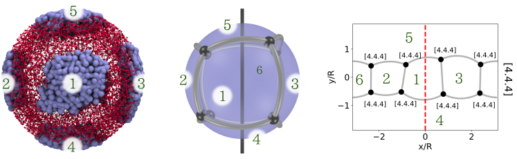
Fig.  4: Spherical tilings from polymeric self-assembly on a spherical substrate Left panel: A simulation snapshot of an equilibrated $ABB$ star copolymer melt confined to a spherical shell. The $A$-type arms have assembled into six domains, which arranged in a cuboidal symmetry in the $B$-type matrix. Middle panel: The spherical tiling recovered from the polymer system. Each face in the tiling corresponds to a blue domain in the simulation snapshot as labeled. Right panel: A modified Mercator projection of the spherical tiling, labeled with the corresponding tiles on the sphere and the domain in the simulation snapshot. Each vertex is labeled with its Schläfli symbol, the union of all types of distinctive vertex labels gives the Schläfli symbol of the entire tiling, as shown vertically on the far right. In order to be comparable, all tilings are rotated so all tilings of a type have the same orientation. The gray axis in the middle panel indicates the orientation of the red, dashed line in the projection in 3D.

For the $ABC$ systems we analyse each of the three species individually, treating the respective other two domains as the matrix, and apply the same analysis as above. That is, to analyse $A$, we consider $B$ and $C$ indistinguishable and to represent the matrix and so on. From each $ABC$ system three tilings from the $A$, $B$ and $C$ type domains are obtained, as can be seen in fig. (6). Tilings are labeled using Schläfli Symbols, see caption of table 1 for details. All simulation screenshots were made using the Tachyon render ⁶⁴ in vmd ⁶⁵, the renderings of the tilings were created using a custom script in blender ⁶⁶.

Every $1\times 10^{6}$ simulation step, a snapshot of all particles was made, which results in 300 frames over the simulation time. The statistics shown in the result section include all tilings from the latest 15 frames of the simulation to account for invalid simulation frames. Since 20 independent rubs were made for each radius, 300 frames were analysed for both the $ABC$ and $ABB$ systems. In the $ABB$ system, this provides 300 spherical tilings, in the $ABC$ system 900 tilings, since there are three colors in each frame. Note, however, that the “real” statistics are only based on 20 different runs for each polymer type and radius, since the tiling in the last 15 frames of each run are assumed to be equilibrated and therefore is not expected to change.

3 Results and discussion

We find the following key features:

Fig.  5: Equilibrium configurations of self-assembly of star copolymers on a spherical substrate Results of multiple runs of the self-assembly of $ABB$ (top) and $ABC$ (bottom) star copolymers on a spherical substrate of radius R. Each color denotes one type of tiling, as labeled in table 1. The plot shows the fraction of simulation snapshots found with the respective tiling for each radius. In general, multiple tilings are found as solutions for a single radius, where the results for $ABB$ and $ABC$ systems differ.

number of tiles with N Schläfli symbol 1 2 3 4 5 6 edges /   [1.1] 2 \   [2.2.2] 3 |   [3.3.3] 4 -   [3.4.4] 2 3 +   [4.4.4] 6 x   [4.4.5] 5 2 o   [[4.4.5], [4.5.5]] 4 4 O   [[4.5.5, 5.5.5]] 3 6 .  0 [[4.5.5, 5.5.5]] 2 8  1 [[4.5.5], [4.5.6], 2 8 1 [5.5.5], [5.5.6]] /\  2 [5.5.5] 12  Non-Thomson  Invalid Table 1: Solutions of the Thomson problem for systems with up to 12 electrons described as spherical tilings. The table shows the number of $n$-gons and the Schläfli symbol for the dual lattice of a solution of a $N$-electron Thomson problem. A Schläfli symbol 67, 12, 68 is a set of $l$ numbers $[k_{1},k_{2},...k_{l}]$ denoting that a vertex is adjacent to $l$ tiles with $k_{l}$ edges respectively (see also right pane in fig. (4)). The Schläfli symbol for an entire tiling just lists all different types of occurring vertices, see fig. (4). The symbols to the left relates to the textures in fig. (5).

• For spherical substrates with $R<8$ all tilings generated by both the $ABB$ and $ABC$ systems are identical to tilings generated from Thomson solutions, see fig. (5). Only for radii $R\geq 8$, we observed simulations of $ABC$ systems which were not Thomson-type solutions (see below). We only found Thomson solutions for the $ABB$ systems.

• For $R>4$, instead of a single equilibrium solution, we find a spectrum of configurations, see fig. (5). Within our analysis, these appear as degenerate (or nearly degenerate) configurations that occur with statistical frequencies.

• The analysis of the three colors of an $ABC$ tiling shows that they each individually form Thomson solutions, but not necessarily of the same tessellation type, see fig. (6).

• The resulting tilings can be tuned by varying the radius of the sphere where the $ABC$ star copolymer system shows a different behaviour in the frequencies of the tilings than the $ABB$ star copolymer systems, see fig. (5).

To start our discussion we single out the $R=8$ systems to illustrate the key results. Out of the 300 frames in the $ABB$ systems with $R=8$, we find the majority of frames (about 95 %) to have 6 tiles in a $[4.4.4]$ configuration, only a very small proportions of 5 % has 5 tiles in a $[3.4.4]$ tiling. Both of the configurations are identical to tilings generated by Thomson solutions. The $ABC$ case is slightly more complex: out of the 900 analysed tilings, we find only about 14 % of the configuration with 6 tiles in a $[4.4.4]$ tiling, 47 % with 7 tiles in a $[4.4.5]$ tiling, about 31 % with 8 tiles in a $[4.4.5,4.5.5]$ tiling and 6 % with 9 tiles as a $[4.5.5,5.5.5]$ configuration. As in the $ABB$ systems, all of these are identical to tilings from Thomson solutions. Only about 1 % of the tilings were found to differ from the Thomson solution tilings.

While for $R=8$ the $ABB$ system overwhelmingly forms the same type of tiling, the $ABC$ misses this feature. We find this behaviour across most of the other systems on different radii: all of the $ABB$ systems form at least two different tilings for each radius, the $R=9$ system even three, however, all are Thomson solutions. All $ABC$ systems show at least three different tilings for each radius, again almost all of them are Thomson solutions. We find exceptions for the $R=4$ spheres, where for both systems only a single type of tiling is found and the $ABC$ system for $R=7$, where although three different tilings are found, the majority (86 %) of analysed frames forms only one type. Another exception are larger $ABC$ systems, where we find an increasing number ($\approx$1% for $R=8$, $\approx$12 % for $R=9$, $\approx$44 % for $R=10$) of tilings not connected to the Thomson problem. However, we do see these percentages go down as the simulations are running for longer times so we conjecture that eventually all non-Thomson solutions might anneal out.

Since the free energy levels of different tilings is a function of the sphere radius, as will be discussed later, this may allow the conclusion that the energy levels are almost degenerate for the majority of the combinations of the chosen star copolymers and simulation volume geometry. The finite temperature of our simulation then allows the system to jump into local minima instead of the energetic ground state, which results in the spectrum of tilings found here. For some systems though ($R=4$, $ABB$ on $R=7$, $ABC$ on $R=8$) the energy level of certain configurations seems to be deep enough to prevent other structures to assemble.

For all of the $ABB$ system and $ABC$ systems with $R<8$ we find that all tilings are of Thomson-type solutions, as seen in fig. (5). This means that the $N$ $A$-type (and respectively $B$- and $C$-type) patches will sit at the same positions as the electrons would in a $N$-electron Thomson solution, which we checked by visual observation. This is a remarkable result since although the polymers only have short range interactions a structure of long range order is formed. Such long range interactions in a similar system of interacting micelles formed by diblock copolymers has been predicted by ⁶⁹.

For $ABC$ systems, with increasing radii beginning at $R\geq 8$ an increasing number of configurations, up to $\approx 40$ % are not of the Thomson-type. However, we argue that these systems are stuck in local minima. The Thomson problem in general is known for its high probability of being stuck in local minima³⁹. Already for $N=32$ electrons the probability of finding the global minimum drops significantly, which roughly coincides with the threshold where our results show local minima. Using polymer melts instead of point-like particles adds even more complexity to the energy landscape. The fact that the $ABB$ systems - somewhat simpler than the $ABC$ system, due to the missing color constraint for example - do not show any non-Thomson solutions and that the proportion of non-Thomson solutions increase with increasing radius, and thus number of patches, supports this.

Based on the observation that the simulations only show Thomson solutions up to systems with $R=7$, all of those $ABC$ systems must consist of three different tilings, each of which solves the Thomson problem on its own while coexisting with two others on the same sphere. We will elaborate on this again using an example system from the $R=8$ runs using fig. (6), however, all systems of various sizes share the same behaviour.

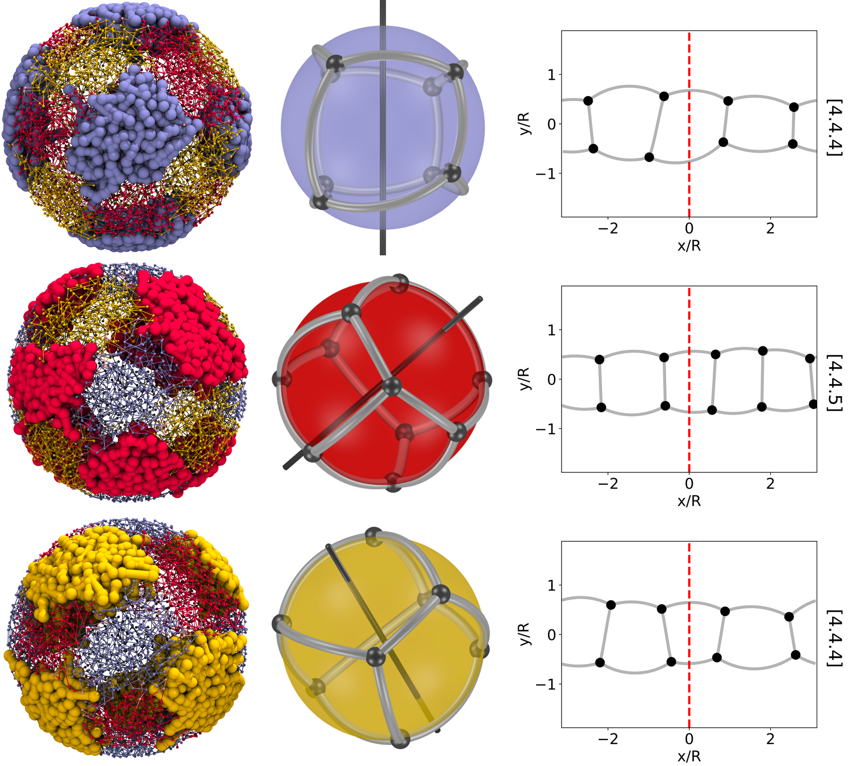
Fig.  6: The three spherical tilings representing the structure of the A, B and C domains The figure shows three tilings, generated by the self-assembly of $ABC$ star copolymers, in each of the colors on the same sphere. Left column: Rendering of the simulation snapshot where the patches creating the tiling are emphasized while showing the others simultaneously. Middle column: The tiling derived from the emphasized patch configuration on the left. The axis shows the orientation of the axis with the highest symmetry. Right column: A 2D projection of the tiling. The black axis in the middle column indicates the position of the red line in the projection plots. The label of the tiling is given on the far right side.

Figure (6) shows how three different Thomson solutions can coexist on a single sphere. When only considering the blue patches, while red and yellow act as a matrix, the resulting tiling is of type $[4.4.4]$. Analogue type $[4.4.5]$ and $[4.4.4]$ tilings are formed in the red and yellow patches respectively. The tilings have a different orientation on the sphere as can be seen on the orientation of the axis of highest symmetry.

In the case of the $R=8$ tilings, the overwhelming number of $ABC$ systems were found to be a combination of three Thomson solutions, where the most prominent combinations are $(7/8/8)$ with 19 %, $(7/7/8)$ with 15 %, $(7/7/7)$ with 15 % and $(6/7/7)$ with 14 %. The number denotes the number of patches in the tiling, the tiling label can be found using table 1. Only a small number of 1 % of the systems contained tilings which are not Thomson solutions. The same holds for systems with smaller radius: since no tilings were found not to solve the Thomson problem, all combinations there consist of Thomson solutions. For larger systems the number of non-Thomson configuration increases. Therefore, the amount of configurations containing non-Thomson solutions increases as well, however, we cannot say if that is caused by increasingly difficult equilibration or due to other reasons, for example the color constraint preventing some combinations to be assembled.

In the $R=8$ case we found the $(7/7/7)$ combination formed in two different ways: once with only Thomson solutions, and once with one Thomson problem configuration and two non-Thomson tilings. In this case we clearly see that it is possible to build this $(7/7/7)$ combination using only Thomson solutions. This hints towards our guess that combinations with non-Thomson solutions are not caused by the color constraint but equilibration issues. Based on the data and this assumption we suspect that the color constraint on its own does not influence the resulting tiling. Apart from this observation we could not find any regularities in the frequencies of the different combinations of the tilings for any radius.

Having said that the color constraint seems to not have any effect on the resulting tilings, it is important to note that although the simulation data of $ABB$ systems for $R=8$ clearly shows the type $[4.4.4]$ tiling as the minimal energy configuration, we could only find one out of 300 combinations being a $3\times[4.4.4]$ tiling on a single sphere in the $ABC$ systems of the same radius. Therefore this finding cannot be a result from the imposed color constraint but must rather be caused by a change in the energy functional.

This observation is found as general behaviour across all runs: there are statistically significant differences in the frequency with which tilings occur in $ABB$ and $ABC$ systems. Therefore, the self-assembly process of ABB and ABC does show differences that are manifested in the topology of the adopted structures, or at least in the statistical properties of these properties. This observation enables us to answer the following question: if one is only able to see one kind of color, for example by looking through colored filters, is it possible to determine if the observed structure is assembled by an $ABB$ or an $ABC$ system? The answer depends on the circumstances: if only one configuration is available, the answer is no, since each configuration found in this article is assembled by both the $ABB$ and the $ABC$ systems. However, if multiple samples are available, the answer is yes. The different statistics of frequencies of the tilings in the different systems as shown in fig. (6) enables us to determine the type of systems of the given samples.

When assuming that all equilibrium solutions are Thomson solutions, the resulting tiling type is determined by the number of patches assembled in the melt. As can be seen in the data, this number is a function of the radius: with increasing sphere size the number of patches increases. This follows from the energy functional of polymer melts in the strong segregation limit:

$$F=F_{\text{conf}}+F_{\text{int}}$$

where $F_{\text{conf}}$ is the entropic contribution determined by the domain shape and $F_{\text{int}}$ is the enthalpic contribution and measures the interface area ⁶⁹. The entropic contribution favours most spherical patch shapes and penalises domains, where the polymer chains have to be stretched. Consider an exemplary $ABB$ system with two $A$-type patches located at the north and south pole of the sphere. The interfaces, on which the grafting points of the star copolymers must sit, are then disk segments centred around the poles. From there the $B$ type arms stretch to cover the entire sphere. Since the arm length is kept constant, the arms must stretch increasingly with increasing sphere radius to cover the surface of the sphere. This comes with an entropic penalty. At some point it becomes energetically more favorable to change to a three patch configuration which, despite the increasing interface energy, relaxes the polymer arms and reduces the entropic energy contribution. This interplay between minimising the interface area and entropic energy contribution determines the number of domains and, thus, the resulting structure in these systems.

The differences in the frequencies of tilings in $ABB$ and $ABC$ systems are caused by a modification of the energy functional. While in the $ABB$ systems only $A-B$ interfaces exist, the $ABC$ systems also develop $A-C$ and $B-C$ interfaces, thus, increasing the enthalpic energy contribution. The entropic contribution changes since the grafting points of the star copolymers are not allowed to move freely along the $A-B$ interface but are constrained to $ABC$ triple lines, resulting in more constrained polymer paths leading, presumably, to an entropic penalty.

4 Conclusion and Outlook

In this article the self-assembly of $ABC$ and $ABB$ star copolymers confined to a spherical shell was simulated using DPD molecular dynamics simulations in order to investigate the combined influence of geometric frustration and the color constraint inherent in the $ABC$ system. In bulk simulations, these polymers form columnar phases whose cross sections are 3-colored, planar, hexagonal tiling patterns. The architecture of $ABC$ stars imposes the color constraint onto the resulting structures: only tiles with an even number of edges are allowed where the color of all adjacent tiles must alternate. To differentiate between the influence of the color constraint and the curvature $ABB$ systems were simulated as reference, where the color constraint does not apply.

We can summarise our findings into four core results: (1) apart from kinetically stuck configurations in large $ABC$ systems $(R\geq 8)$, we find all tilings in both $ABB$ and $ABC$ systems to be Thomson solutions. (2) In $ABC$ systems we find three possibly different tilings on each sphere, one in each color while neglecting the other two, all of which solve the Thomson problem for small radii individually. We find some non-Thomson solutions for larger radii ($R\geq 8$) but believe this is due to equilibration issues as discussed above.

(3) A spectrum of configurations dominates the ensemble, rather than a single structure. This leads to the occurrence of a small number of different tilings in both $ABB$ and $ABC$ systems, with varying probability. (4) The latter can be tuned by varying the sphere radius, which means we can switch between Thomson solutions of different numbers of particles. While we could not find any combination of three tilings on the same sphere which the color constraint does not allow, the frequencies of the tilings in the $ABC$ compared to the $ABB$ system show statistically significant differences. This provides the possibility to differentiate between the two systems: statistically speaking we can determine if a tiling was formed by an $ABB$ or and $ABC$ system by only being able to see a single color.

A direct comparison of our work to the presented results of frozen particles on a sphere ³⁴ or the diblock copolymers on a spherical substrate ³⁰ is somewhat difficult: while in these systems the number of particles is in the order of 100 (which is equivalent to one patch in our systems), our largest system consists of a maximum of 12 domains in a single tiling. At these system sizes the tilings are missing the regularity to define “defects” in their structure. Taking the entire $ABC$ system with all of its colors into account, however, we have a system consisting of up to 37 patches. Here we can see the influence of the color constraint: instead of finding isolated pentagonal defects or scars of pentagons and heptagons, we find either six squares or a combination of squares and octagons to cope with the geometrical constraint.

A promising and interesting application of this work can be found in the field of patchy particles: discrete particles with patches on their surface which can couple and form bonds to other patches, e.g. Janus-particles ⁷⁰, ⁷¹. A mechanism to assemble such particles and tune their coordination number include self-assembly of monolayers of surfactants on spherical substrates ⁷², ⁷³. Our work presents an example how such a self-assembly could be realised. Instead of using two repulsive walls to model a spherical substrate, the architecture and composition of the polymer can be modified, so that spherical droplets will form in solution, as seen in previous work⁷⁴, ⁷⁵, ⁷⁶, ⁷⁷. Preliminary simulations showed that adding a fourth arm, immiscible with the already existing arms, would form the core of such a droplet, on which surface the $ABC$ arms assemble as presented in this work. By tuning the length of this fourth arm, the radius of the droplets can be changed. As shown in this article, the number of patches would change and therefore the coordination number of the droplet as a patchy particle. Further, instead of using symmetric star copolymers, the length of one arm can be varied to generate different, ’asymmetric’ tilings, analogue to ¹⁰, ¹².

Conflict of Interest

The Authors declare no conflict of interest.

References

- Bates 2005 F. S. Bates, MRS Bulletin, 2005, 30, 525–532.
- Matsen 2007 M. W. Matsen, in Self Consistent Field Theory and Its Applications, Wiley-Blackwell, 2007, ch. 2, pp. 87–178.
- Grason and Kamien 2004 G. M. Grason and R. D. Kamien, Macromolecules, 2004, 37, 7371–7380.
- Polymeropoulos et al. 2017 G. Polymeropoulos, G. Zapsas, K. Ntetsikas, P. Bilalis, Y. Gnanou and N. Hadjichristidis, Macromolecules, 2017, 50, 1253–1290.
- Guo et al. 2008 Z. Guo, G. Zhang, F. Qiu, H. Zhang, Y. Yang and A.-C. Shi, Phys. Rev. Lett., 2008, 101, 028301.
- Tyler et al. 2007 C. A. Tyler, J. Qin, F. S. Bates and D. C. Morse, Macromolecules, 2007, 40, 4654–4668.
- Fischer et al. 2014 M. G. Fischer, L. de Campo, J. J. K. Kirkensgaard, S. T. Hyde and G. E. Schröder-Turk, Macromolecules, 2014, 47, 7424–7430.
- Okamoto et al. 1997 S. Okamoto, H. Hasegawa, T. Hashimoto, T. Fujimoto, H. Zhang, T. Kazama, A. Takano and Y. Isono, Polymer, 1997, 38, 5275 – 5281.
- Kirkensgaard and Hyde 2009 J. J. K. Kirkensgaard and S. Hyde, Phys. Chem. Chem. Phys., 2009, 11, 2016–2022.
- Kirkensgaard et al. 2014 J. J. K. Kirkensgaard, M. C. Pedersen and S. T. Hyde, Soft Matter, 2014, 10, 7182–7194.
- Kirkensgaard 2012 J. J. K. Kirkensgaard, Interface Focus, 2012, 2, 602–607.
- Gemma et al. 2002 T. Gemma, A. Hatano and T. Dotera, Macromolecules, 2002, 35, 3225–3237.
- de Campo et al. 2011 L. de Campo, T. Varslot, M. J. Moghaddam, J. J. K. Kirkensgaard, K. Mortensen and S. T. Hyde, Phys. Chem. Chem. Phys., 2011, 13, 3139–3152.
- Hayashida et al. 2007 K. Hayashida, T. Dotera, A. Takano and Y. Matsushita, Phys. Rev. Lett., 2007, 98, 195502.
- Hayashida et al. 2006 K. Hayashida, W. Kawashima, A. Takano, Y. Shinohara, Y. Amemiya, Y. Nozue and Y. Matsushita, Macromolecules, 2006, 39, 4869–4872.
- Takano et al. 2004 A. Takano, S. Wada, S. Sato, T. Araki, K. Hirahara, T. Kazama, S. Kawahara, Y. Isono, A. Ohno, N. Tanaka and Y. Matsushita, Macromolecules, 2004, 37, 9941–9946.
- Takano et al. 2005 A. Takano, W. Kawashima, A. Noro, Y. Isono, N. Tanaka, T. Dotera and Y. Matsushita, Journal of Polymer Science Part B: Polymer Physics, 2005, 43, 2427–2432.
- Tang et al. 2004 P. Tang, F. Qiu, H. Zhang and Y. Yang, The Journal of Physical Chemistry B, 2004, 108, 8434–8438.
- Zhang et al. 2010 G. Zhang, F. Qiu, H. Zhang, Y. Yang and A.-C. Shi, Macromolecules, 2010, 43, 2981–2989.
- Matsushita 2007 Y. Matsushita, Macromolecules, 2007, 40, 771–776.
- Kirkensgaard 2012 J. J. K. Kirkensgaard, Phys. Rev. E, 2012, 85, 031802.
- Irvine et al. 2010 W. T. M. Irvine, V. Vitelli and P. M. Chaikin, Nature, 2010, 468, 947.
- Irvine et al. 2012 W. T. M. Irvine, M. J. Bowick and P. M. Chaikin, Nature Materials, 2012, 11, 948–51.
- Guerra et al. 2018 R. E. Guerra, C. P. Kelleher, A. D. Hollingsworth and P. M. Chaikin, Nature, 2018, 554, 346.
- Lipowsky et al. 2005 P. Lipowsky, M. J. Bowick, J. H. Meinke, D. R. Nelson and A. R. Bausch, Nature Materials, 2005, 4, 407–11.
- Einert et al. 2005 T. Einert, P. Lipowsky, J. Schilling, M. J. Bowick and A. R. Bausch, Langmuir, 2005, 21, 12076–12079.
- Bausch et al. 2003 A. R. Bausch, M. J. Bowick, A. Cacciuto, A. D. Dinsmore, M. F. Hsu, D. R. Nelson, M. G. Nikolaides, A. Travesset and D. A. Weitz, Science, 2003, 299, 1716–1718.
- Giarritta et al. 1992 S. P. Giarritta, M. Ferrario and P. Giaquinta, Physica A: Statistical Mechanics and its Applications, 1992, 187, 456 – 474.
- Giarritta et al. 1993 S. Giarritta, M. Ferrario and P. Giaquinta, Physica A: Statistical Mechanics and its Applications, 1993, 201, 649 – 665.
- Zhang et al. 2014 L. Zhang, L. Wang and J. Lin, Soft Matter, 2014, 10, 6713–6721.
- Kamien 2002 R. D. Kamien, Rev. Mod. Phys., 2002, 74, 953–971.
- Bowick and Giomi 2009 M. J. Bowick and L. Giomi, Advances in Physics, 2009, 58, 449–563.
- Conway et al. 2016 J. Conway, H. Burgiel and C. Goodman-Strauss, The Symmetries of Things, CRC Press, 2016.
- Bowick et al. 2000 M. J. Bowick, D. R. Nelson and A. Travesset, Phys. Rev. B, 2000, 62, 8738–8751.
- Bowick et al. 2002 M. Bowick, A. Cacciuto, D. R. Nelson and A. Travesset, Phys. Rev. Lett., 2002, 89, 185502.
- Bowick and Yao 2011 M. J. Bowick and Z. Yao, EPL (Europhysics Letters), 2011, 93, 36001.
- Thomson 1904 J. J. Thomson, The London, Edinburgh, and Dublin Philosophical Magazine and Journal of Science, 1904, 7, 237–265.
- Erber and Hockney 1991 T. Erber and G. M. Hockney, Journal of Physics A: Mathematical and General, 1991, 24, L1369.
- Bondarenko et al. 2015 A. N. Bondarenko, M. N. Karchevskiy and L. A. Kozinkin, Journal of Physics: Conference Series, 2015, 643, 012103.
- Altschuler et al. 1997 E. L. Altschuler, T. J. Williams, E. R. Ratner, R. Tipton, R. Stong, F. Dowla and F. Wooten, Phys. Rev. Lett., 1997, 78, 2681–2685.
- Wales and Ulker 2006 D. J. Wales and S. Ulker, Phys. Rev. B, 2006, 74, 212101.
- Wales et al. 2009 D. J. Wales, H. McKay and E. L. Altschuler, Phys. Rev. B, 2009, 79, 224115.
- Caspar and Klug 1962 D. L. D. Caspar and A. Klug, Cold Spring Harbor Symposia on Quantitative Biology, 1962, 27, 1–24.
- Mannige and Brooks 2008 R. V. Mannige and C. L. Brooks, Phys. Rev. E, 2008, 77, 051902.
- Rochal et al. 2016 S. B. Rochal, O. V. Konevtsova, A. E. Myasnikova and V. L. Lorman, Nanoscale, 2016, 8, 16976–16988.
- Robinson et al. 2013 M. Robinson, I. Suarez-Martinez and N. A. Marks, Phys. Rev. B, 2013, 87, 155430.
- Mughal 2014 A. Mughal, Forma, 2014, 29, 13–19.
- Pérez-Garrido et al. 1997 A. Pérez-Garrido, M. J. W. Dodgson and M. A. Moore, Phys. Rev. B, 1997, 56, 3640–3643.
- Hoogerbrugge and Koelman 1992 P. J. Hoogerbrugge and J. M. V. A. Koelman, EPL (Europhysics Letters), 1992, 19, 155.
- Español and Warren 1995 P. Español and P. Warren, EPL (Europhysics Letters), 1995, 30, 191.
- Kirkensgaard 2010 J. J. K. Kirkensgaard, Soft Matter, 2010, 6, 6102.
- Kirkensgaard 2011 J. J. K. Kirkensgaard, Soft Matter, 2011, 7, 10756.
- Anderson et al. 2008 J. A. Anderson, C. D. Lorenz and A. Travesset, Journal of Computational Physics, 2008, 227, 5342 – 5359.
- Glaser et al. 2015 J. Glaser, T. D. Nguyen, J. A. Anderson, P. Lui, F. Spiga, J. A. Millan, D. C. Morse and S. C. Glotzer, Computer Physics Communications, 2015, 192, 97 – 107.
- Phillips et al. 2011 C. L. Phillips, J. A. Anderson and S. C. Glotzer, Journal of Computational Physics, 2011, 230, 7191 – 7201.
- Groot and Warren 1997 R. D. Groot and P. B. Warren, The Journal of Chemical Physics, 1997, 107, 4423–4435.
- 57 https://hoomd-blue.readthedocs.io/en/stable/index.html.
- Flory 1942 P. J. Flory, The Journal of Chemical Physics, 1942, 10, 51–61.
- Huggins 1942 M. L. Huggins, Annals of the New York Academy of Sciences, 1942, 43, 1–32.
- Groot and Madden 1998 R. D. Groot and T. J. Madden, The Journal of Chemical Physics, 1998, 108, 8713–8724.
- Schaller et al. 2013 F. M. Schaller, S. C. Kapfer, M. E. Evans, M. J. Hoffmann, T. Aste, M. Saadatfar, K. Mecke, G. W. Delaney and G. E. Schröder-Turk, Philosophical Magazine, 2013, 93, 3993–4017.
- Weis, Simon et al. 2017 Weis, Simon, Schönhöfer, Philipp W. A., Schaller, Fabian M., Schröter, Matthias and Schröder-Turk, Gerd E., EPJ Web Conf., 2017, 140, 06007.
- 63 freud, https://freud.readthedocs.io/en/stable/index.html, Accessed: 2019-01-17.
- Stone 1998 J. Stone, MSc thesis, Computer Science Department, University of Missouri-Rolla, 1998.
- Humphrey et al. 1996 W. Humphrey, A. Dalke and K. Schulten, Journal of Molecular Graphics, 1996, 14, 33–38.
- 66 blender, https://www.blender.org/.
- Kirkensgaard et al. 2014 J. J. K. Kirkensgaard, M. E. Evans, L. de Campo and S. T. Hyde, Proceedings of the National Academy of Sciences, 2014, 111, 1271–1276.
- Grünbaum and Shephard 2013 B. Grünbaum and G. Shephard, Tilings and Patterns, Dover Publications, Incorporated, 2013.
- Semenov 1985 A. Semenov, Journal of Experimental and Theoretical Physic, 1985, 61, 744.
- Zhang and Glotzer 2004 Z. Zhang and S. C. Glotzer, Nano Letters, 2004, 4, 1407–1413.
- Casagrande et al. 1989 C. Casagrande, P. Fabre, E. Raphaël and M. Veyssié, Europhysics Letters (EPL), 1989, 9, 251–255.
- Pons-Siepermann and Glotzer 2012 I. C. Pons-Siepermann and S. C. Glotzer, Soft Matter, 2012, 8, 6226–6231.
- Pons-Siepermann and Glotzer 2012 I. C. Pons-Siepermann and S. C. Glotzer, ACS Nano, 2012, 6, 3919–3924.
- Higuchi et al. 2008 T. Higuchi, A. Tajima, K. Motoyoshi, H. Yabu and M. Shimomura, Angewandte Chemie International Edition, 2008, 47, 8044–8046.
- Higuchi et al. 2008 T. Higuchi, A. Tajima, H. Yabu and M. Shimomura, Soft Matter, 2008, 4, 1302–1305.
- Jeon et al. 2007 S.-J. Jeon, G.-R. Yi, C. M. Koo and S.-M. Yang, Macromolecules, 2007, 40, 8430–8439.
- Ku et al. 2019 K. H. Ku, Y. J. Lee, Y. Kim and B. J. Kim, Macromolecules, 2019, 52, 1150–1157.