Geometrical and spectral study of -skeleton graphs
Abstract
We perform an extensive numerical analysis of -skeleton graphs, a particular type of proximity graphs. In a -skeleton graph (BSG) two vertices are connected if a proximity rule, that depends of the parameter , is satisfied. Moreover, for there exist two different proximity rules, leading to lune-based and circle-based BSGs. First, by computing the average degree of large ensembles of BSGs we detect differences, which increase with the increase of , between lune-based and circle-based BSGs. Then, within a random matrix theory (RMT) approach, we explore spectral and eigenvector properties of randomly weighted BSGs by the use of the nearest-neighbor energy-level spacing distribution and the entropic eigenvector localization length, respectively. The RMT analysis allows us to conclude that a localization transition occurs at .
pacs:
89.75.Hc, 64.60.-i, 05.45.MtI Introduction
The analysis of spatial networks plays a fundamental role for understanding complex systems embedded in geographical spaces, see B11 ; B18 . Here we study a model which is a generalization of the so-called random neighborhood graphs DGKJDR ; GTT , known as -skeleton graphs, embedded in the unit square. In a -skeleton graph (BSG) two vertices (points or nodes) are connected by an edge if and only if these vertices satisfy a particular geometrical requirement named as proximity rule. The proximity rule is encoded in the parameter which takes values in the interval . With the proximity rules we will define below, a fully connected graph is obtained in the limit , while the network becomes a disconnected graph when .
In particular, BSGs are useful to study geometric complex systems where the connectivity between two items is interfered by the presence of a third one in between them. This is the case, for instance of granular materials BOD12 , for representing urban street networks OH14 , as well as for representing fractures in rocks estrada , among others.
This work is organized as follows. In Sec. II we introduce the proximity rules needed to construct the BSGs. In fact, for there exist two different proximity rules, leading to lune-based and circle-based BSGs. Indeed, our study focus on a detailed comparison between both. Therefore, we study topological and spectral properties of BSGs by the use of the average degree, in Sec. III, and nearest-neighbor energy-level spacing distribution and the entropic eigenvector localization length, in Sec. IV. Finally, we summarize in Sec. V.
II Definitions of -skeleton graphs
For a given set of vertices on the plane, an Euclidean distance function , and a parameter , a graph , called BSG, is defined as follows DGKJDR :
Two vertices are connected with an edge iff no point from \ belongs to the neighborhood , where:
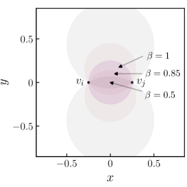
(1) for , is the intersection of two discs, each with radius
| (1) |
having the segment as a chord. The disc centers are located at
| (2) |
where is a rotation matrix and and are the coordinate vectors of the corresponding vertices, namely
| (3) |
In Fig. 1 we show some examples of neighborhoods . We stress that in the limit the neighborhood becomes the straight line joining the vertices and , so the network becomes fully connected.
(2) for there are two proximity rules:
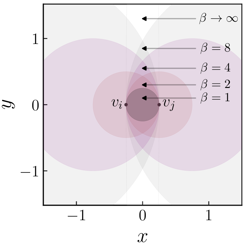
(2a) lune-based BSG. Here is the intersection of two discs, each with radius
| (4) |
whose centers are at
| (5) | ||||
| (6) |
In Fig. 2(a) we can see the lunes of influence for different values of . Note that in the limiting case , is an infinite strip of width ; thus, even for very large values of some connections may exist.
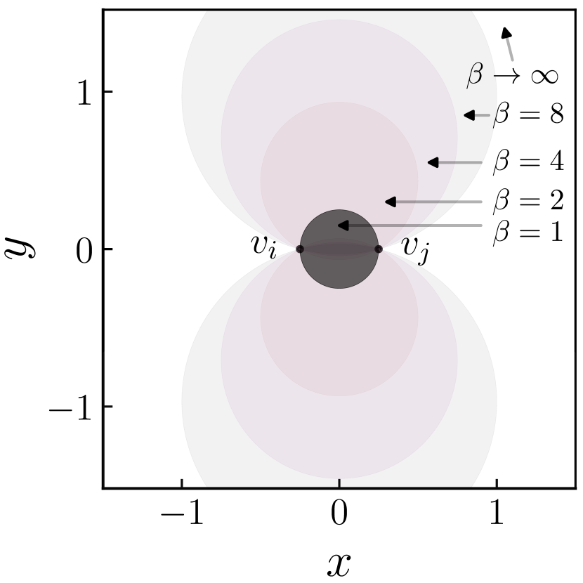
(2b) circle-based BSG. Here is the union of two discs, with radius given by Eq. (4), that pass through both and . The disc centers are located at
| (7) |
In Fig. 2(b) we can see the circles of influence for different values of . Note that in the limiting case , is the entire plane; therefore, for large enough values of the skeleton graph becomes a disconnected graph.
It is worth mentioning that for , Eqs. (2), (5) and (7) reduce to the same expression. Indeed, the case is well known in the literature as Gabriel graph KRRRS and addressed as a -skeleton graph. Another well known case is , which is known as relative neighborhood graph GTT , in the lune-based formulation, and typically addressed as -skeleton graph.
(a)
(b)
III Random -skeleton graphs in the unit square
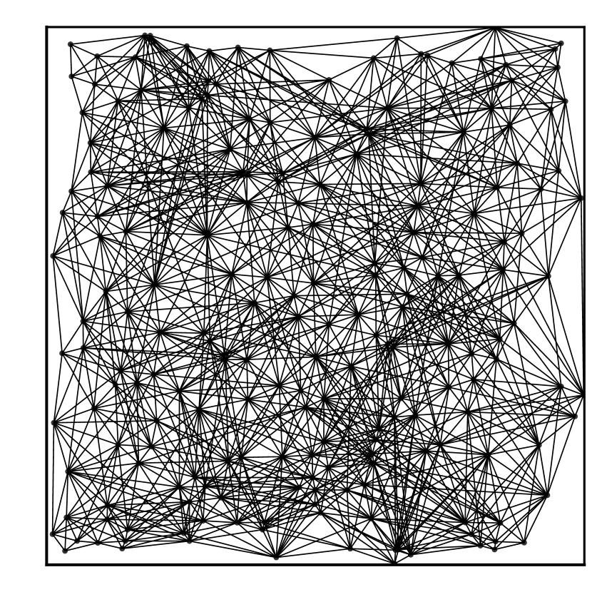
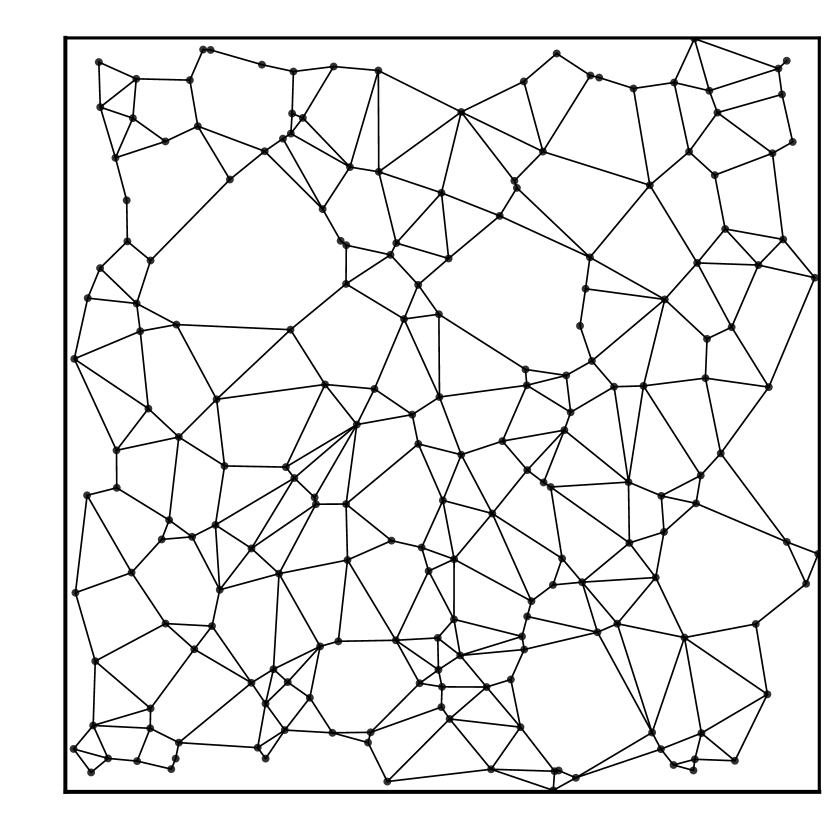
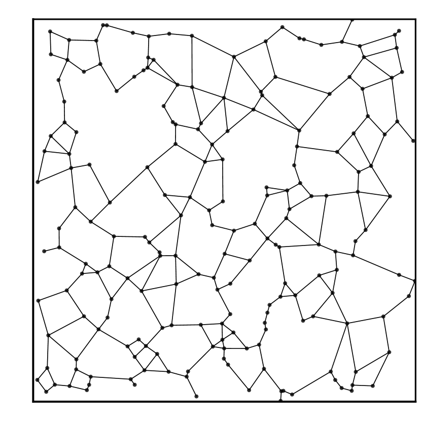
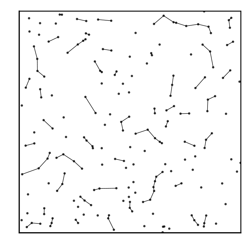
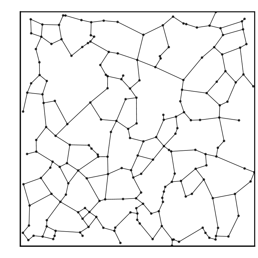
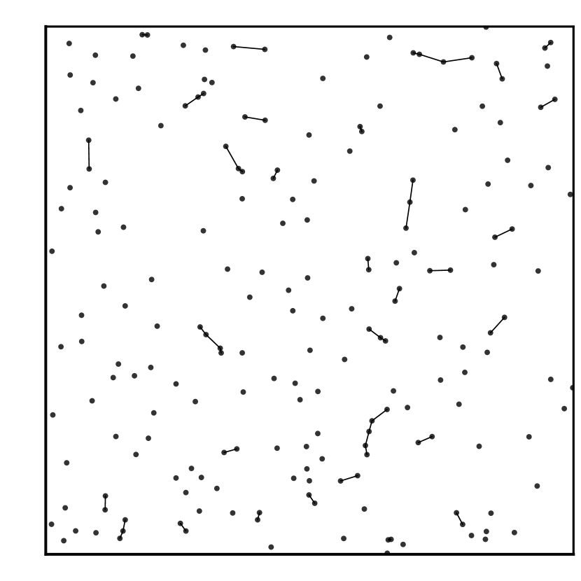
In this work we consider randomly and independently distributed vertices in the unit square. As examples, in Fig. 3 we show BSGs with and for . Note that we have used the same set of randomly distributed vertices in both panels. Here, since the proximity rule is unique. Then, in Fig. 4 we present BSGs for and . There we consider both the lune-based (left panels) and the circle-based (right panels) proximity rules. We have used the same set of vertices of Fig. 3. From this figure it is clear that different proximity rules produce quite different networks. In particular, for a fixed value of , lune-based skeleton graphs show higher connectivity than circle-based skeleton graphs. We will characterize this feature by the use of geometrical and spectral properties below.
III.1 Average degree
A well known topological measure in graph theory is the degree of a vertex , which is the number of edges incident to a given vertex. Here, since we are interested in random BSGs, we will consider the ensemble average degree that we compute by averaging over all vertices of BSGs with fixed parameter pairs .
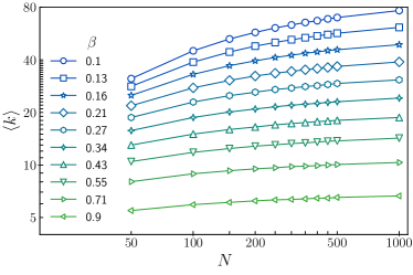
On the one hand, in Figs. 5 we plot as a function of for random BSGs with several values of (i.e., when only one proximity rule applies). We observe that for fixed , increases for increasing . Moreover, for fixed , increases for decreasing ; this confirms the expected scenario of completely connected networks in the limit .
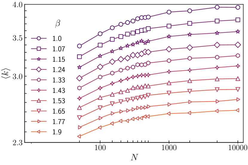
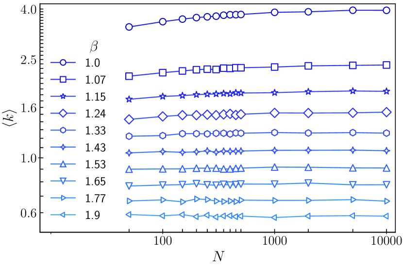
On the other hand, in Figs. 6 and 7 we also plot as a function of but now for random BSGs with . We consider both lune-based (left panels) and circle-based (right panels) proximity rules. For clarity, we group the data in the regimes (Fig. 6) and (Fig. 7). First, let us concentrate on the BSGs constructed with the lune-based proximity rule, see left panels in Figs. 6 and 7. There, we observe three different behaviors for : (i) when is small, , is an increasing function of ; (ii) for intermediate values of , , is approximately constant for the values of we used in this work; and (iii) when is large, , is a decreasing function of . This panorama is also observed for BSGs constructed with the circle-based proximity rule (see right panels in Figs. 6 and 7) however shifted to smaller values of ; that is, is approximately constant as a function of for .
(a)
(b)
(a)
Lune-based BSGs
(b)
Circle-based BSGs
(c)
(d)
(a)
Lune-based proximity rule
(b)
Circle-based proximity rule
(a)
Lune-based proximity rule

(b)
Circle-based proximity rule

From the observations above we can concluded that for intermediate values of (including relative neighbor graphs) the BSGs are very stable graphs in the sense that the average degree remains constant even in the presence of strong vertex density fluctuations.
The main difference we can observe between random BSGs constructed with the lune-based and circle-based proximity rules is that in the circle-based case the networks become disconnected for relatively smaller values of than in the lune-based case; compare Figs. 7(a) and 7(b) and also left and right panels in Fig. 4. Indeed, from Fig. 7(b) it is clear that when it is highly probable to have completely disconnected networks.
IV Weighted random -skeleton graphs
Here, in order to use Random Matrix Theory (RMT) results as a reference, we include weights, particularly random weights, to the random BSGs defined above. Specifically, we choose the non-vanishing elements of the corresponding adjacency matrices to be statistically independent random variables drawn from a normal distribution with zero mean and variance , where is the Kronecker delta. Therefore, a diagonal adjacency random matrix is obtained for isolated vertices (known in RMT as the Poisson case), whereas the Gaussian Orthogonal Ensemble (GOE) is recovered when the graph is fully connected.
Below we use exact numerical diagonalization to obtain the eigenvalues and eigenvectors () of the adjacency matrices of large ensembles of weighted random BSGs characterized by and .
IV.1 Spectral properties
In order to characterize the spectra of weighted random BSGs, we use the nearest-neighbor energy level spacing distribution metha ; a widely used tool in RMT. For , i.e., when the vertices in the random BSGs are mostly isolated, the corresponding adjacency matrices are almost diagonal and, regardless of the size of the graph, should be close to the exponential distribution,
| (8) |
which is better known in RMT as Poisson distribution. In the opposite limit, , when the weighted BSGs are fully connected, the adjacency matrices become members of the GOE (real and symmetric full random matrices) and closely follows the Wigner-Dyson distribution,
| (9) |
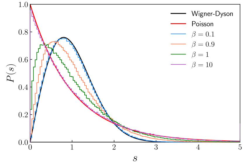
Thus, for a fixed graph size , by increasing from zero to infinity, the shape of is expected to evolve from the Wigner-Dyson distribution to the Poisson distribution. Moreover, for a fixed value of , the increase in the density of vertices also produces changes in the shape of . In Fig. 8 we explore both scenarios.
(a)
(b)
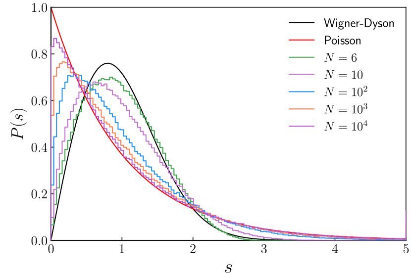
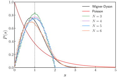
We construct histograms of from unfolded spacings metha , , around the band center of a large number of graph realizations (such that all histograms are constructed with spacings). Here, is the mean level spacing computed for each adjacency matrix. Then, Fig. 8 presents histograms of for the adjacency matrices of weighted random BSGs: In Fig. 8(a) the graph size is fixed to and takes the values 0.1, 0.9, 1, and 10. In this figure we observe a complete transition in the shape of from the Wigner-Dyson to Poisson distribution functions (also shown as reference) for increasing . In Fig. 8(b) the parameter is set to one (Gabriel graph) while increases from 6 to . Here, in contrast to Fig. 8(a), we do not observe a complete transition from Wigner-Dyson to Poisson in the shape of . From Fig. 8(b) one may expect that by decreasing further the number of vertices the Wigner-Dyson shape could emerge; however, this is not the case, as shown in Fig. 9. There we observe that for the becomes symmetric with respect to . It is important to stress that we have nor observed this shape for the before. Indeed, in other random network models embedded in the plane, such as random regular graphs and random rectangular graphs (RRGs) (for the definition and general properties of RRGs the reader is referred to ES15 ), we did observe the full transition from Wigner-Dyson to Poisson for the as a function of the density of vertices for a fixed value of the proximity rule parameter AMGM18 .
Now, in order to characterize the shape of for weighted random BSGs we use the Brody distribution B73 ; B81
| (10) |
where , is the gamma function, and , known as Brody parameter, takes values in the range . Equation (10) was originally derived to provide an interpolation expression for in the transition from Poisson to Wigner-Dyson distributions, serving as a measure for the degree of mixing between Poisson and GOE statistics. In fact, and in Eq. (10) produce Eqs. (8) and (9), respectively. In particular, as we show below, the Brody parameter will allows us to identify the onset of the localization transition for random BSGs. It is also relevant to mention that the Brody distribution has been applied to study other complex networks models, see e.g. AMGM18 ; BJ07 ; JB08 ; ZYYL08 ; J09 ; JB07 ; MAM15 ; DGK16 . In fact, we found that Eq. (10) provides excellent fittings to the histograms of of weighted random BSGs. For example, the fittings to the histograms in Fig. 8(a) [Fig. 8(b)] (not shown to avoid figure saturation) provide: , , , and [, , , , and ]. It is important to remark that for the can not be fitted by the Brody distribution, see Fig. 9, therefore we will not consider small graph sizes in our analysis below.
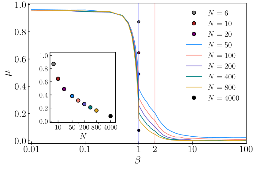
Thus we now perform a systematic study of the Brody parameter as a function of the parameters and of the BSGs. To this end, we construct histograms of for a large number of parameter combinations to extract the corresponding values of by fitting them using Eq. (10). Figure 10 reports versus for five different graph sizes for both proximity rules; lune-based and circle-based. Notice that in all cases the behavior of is similar for increasing : for small (i.e., ) is approximately constant and equal to ; then decreases fast for approaching one; and finally, for , continues decreasing but slowly when is further increased. For large (i.e., ) and large , .
(a)
Lune-based proximity rule
(b)
Circle-based proximity rule
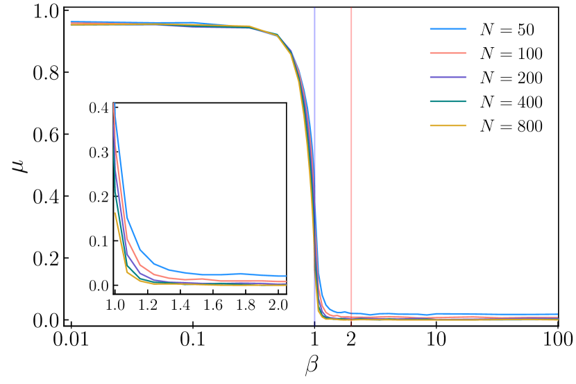
Indeed, from Fig. 10 we can conclude that our model of weighted random BSGs undergoes a clear and sharp transition at from a regime very close to the GOE regime (mostly connected vertices), , to the Poisson regime (mostly isolated vertices), , as a function of . What is remarkable is that this delocalization-to-localization transition seems to be independent of the density of vertices ; in fact, the larger the value of the sharper the transition at is. It is interesting to recall that we have also identified a delocalization-to-localization transition in random regular graphs as a function of the proximity rule parameter AMGM18 ; however, for that model the transition is rather smooth and importantly depends on the density of vertices. In addition, in the inset of Fig. 10(a) we present the values of for increasing for Gabriel graphs where we include the case .
The main difference we can observe between random BSGs constructed with the lune-based and circle-based proximity rules is that the Poisson limit is approached faster in the circle-based case, which was already expected from the analysis of the average degree of the previous Subsection since there it was shown that circle-based BSGs become completely disconnected for relatively smaller values of .
IV.2 Eigenvector properties
(a)
Lune-based proximity rule
(b)
Circle-based proximity rule
The term “localization transition” we used in the previous subsection to describe the sharp decrease of at implies that we expect the eigenvectors of the adjacency matrices of BSGs to be mostly localized for . In the following we verify this statement.
To measure quantitatively the spreading of eigenvectors in a given basis, i.e., their localization properties, two quantities are mostly used: (i) the information or Shannon entropy and (ii) the inverse participation number . Indeed, both have been widely used to characterize the eigenvectors of the adjacency matrices of random network models. For the eigenvector , associated with the eigenvalue , they are given as
| (11) |
and
| (12) |
These measures provide the number of main components of the eigenvector . Moreover, allows to compute the so called entropic eigenvector localization length I90
| (13) |
where is the average entropy of a random eigenvector with Gaussian distributed amplitudes (i.e., an eigenvector of the GOE) which is given by BMHJK
| (14) |
Above, denotes average and is the Digamma function; for large .
We average over all eigenvectors of an ensemble of adjacency matrices of size to compute , such that for each combination we use eigenvectors. With definition (13), when , since the eigenvectors of the adjacency matrices of BSGs have only one main component with magnitude close to one, and . On the other hand, for , and the fully chaotic eigenvectors extend over the available vertices of the BSG, so .
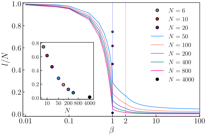
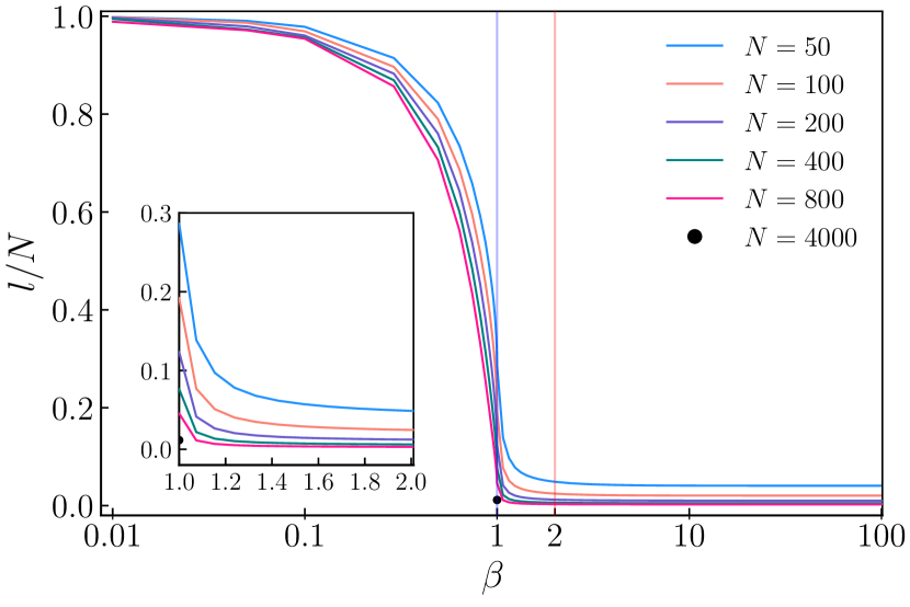
Therefore, in Fig. 11 we plot as a function of for weighted random BSGs of sizes ranging from to 800. We consider both lune-based (Fig. 11(a)) and circle-based (Fig. 11(b)) proximity rules. As well as for the Brody parameter vs. (see Fig. 10) here we clearly observe a sharp transition from delocalized to localized eigenvectors at . Additionally, in the inset of Fig. 11(a) we report vs. for . There we can clearly see the GOE () to Poisson () transition in the eigenvector properties of Gabriel graphs, also reported through spectral properties, by the use of the , see the inset of Fig. 10(b).
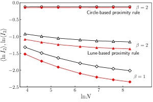
Finally, we would like to add that the inverse participation number of the eigenvectors of BSGs shows an equivalent panorama to that reported in Fig. 11 for , so we do not show it here. Instead, in Fig. 12 we plot and as a function of for Gabriel graphs () and relative neighborhood graphs (). The non-linear trend of the curves corresponding to and in the lune-based proximity rule rejects the possible existence of a localization transition of the Anderson type where the eigenvectors are multifractal objects characterized by a set of dimensions , where the correlation dimension can be extracted from the scalings or ( is known as the typical value of ). See for example Refs. TM16 ; GGG17 ; VMR19 where multifractality of eigenvectors has been reported in random graph models. Moreover the independence of both and on for in the circle-based proximity rule confirms that the corresponding eigenvectors are in the localized regime; that is, .
V Conclusions
In this paper we perform a thorough study of a particular type of proximity graphs known as -skeleton graphs (BSGs). In a BSG two vertices are connected if a proximity rule, that depends of the parameter , is satisfied. We explore the two known versions of them: lune-based and circle-based BSGs.
Our main result is the identification of a delocalization-to-localization transition at for the eigenvectors of the adjacency matrices of BSGs for increasing . It is important to stress that the localized phase corresponds to mostly isolated vertices while the delocalized phase identifies mostly complete graphs, see e.g. AMGM18 ; MAM15 ; VMR19 . We characterize the delocalization-to-localization transition by means of topological and spectral properties; we use the standard average degree as topological measure and, within a random matrix theory approach, the nearest-neighbor energy-level spacing distribution and the entropic eigenvector localization length as spectral measures.
Acknowledgements.
This work was partially supported by VIEP-BUAP (Grant No. 100405811-VIEP2019) and Fondo Institucional PIFCA (Grant No. BUAP-CA-169).References
- (1) M. Barthélémy, Spatial networks, Phys. Rep. 499, 1 (2011).
- (2) M. Barthelemy, Morphogenesis of Spatial Networks, Lecture Notes in Morphogenesis (Springer International Publish, 2018).
- (3) D. G. Kirkpatrick and J. D. Radke, A framework for computational morphology (IBM Thomas J. Watson Research Division, 1984).
- (4) G. T. Toussaint, The relative neighborhood graph of a finite planar set, Pattern Recognition 12, 261 (1980).
- (5) D. S. Bassett, E. T. Owens, K. E. Daniels, and M. A. Porter, Influence of network topology on sound propagation in granular materials, Phys. Rev. E 86, 041306 (2012).
- (6) T. Osaragi and Y. Hiraga, Street network created by proximity graphs: Its topological structure and travel efficiency. In: Proceedings of the 17th Conference of the Association of Geographic Information Laboratories for Europe on Geographic Information Science (AGILE2014), Huerta, Schade, Granell (Eds), pp. 1-6, Castellón, Spain (2014).
- (7) E. Estrada and M. Sheerin, Random neighborhood graphs as models of fracture networks on rocks: Structural and dynamical analysis, Appl. Math. Comp. 314, 360 (2017).
- (8) K. R. Gabriel and R. R. Sokal, A new statistical approach to geographic variation analysis, Systematic Zoology 18, 259 (1969).
- (9) M. L. Mehta, Random matrices (Elsevier, Amsterdam, 2004).
- (10) E. Estrada and M. Sheerin, Random rectangular graphs, Phys. Rev. E 91, 042805 (2015).
- (11) L. Alonso, J. A. Mendez-Bermudez, A. Gonzalez-Melendrez, and Y. Moreno, Weighted random-geometric and random-rectangular graphs: Spectral and eigenvector properties of the adjacency matrix, J. Complex Networks 6, 753 (2018).
- (12) T. A. Brody, A statistical measure for the repulsion of energy levels, Lett. Nuovo Cimento 7, 482 (1973).
- (13) T. A. Brody, J. Flores, J. B. French, P. A. Mello, A. Pandey, and S. S. M. Wong, Random-matrix physics: spectrum and strength fluctuations, Rev. Mod. Phys. 53, 385 (1981).
- (14) J. N. Bandyopadhyay and S. Jalan, Universality in complex networks: Random matrix analysis, Phys. Rev. E 76, 026109 (2007).
- (15) S. Jalan and J. N. Bandyopadhyay, Random matrix analysis of network Laplacians, Physica A 387, 667 (2008).
- (16) G. Zhu, H. Yang, C. Yin, and B. Li, Localizations on complex networks, Phys. Rev. E 77, 066113 (2008).
- (17) S. Jalan, Spectral analysis of deformed random networks Phys. Rev. E 80, 046101 (2009).
- (18) S. Jalan and J. N. Bandyopadhyay, Random matrix analysis of complex networks, Phys. Rev. E 76, 046107 (2007).
- (19) J. A. Mendez-Bermudez, A. Alcazar-Lopez, A. J. Martinez-Mendoza, F. A. Rodrigues, and T. K. DM. Peron, Universality in the spectral and eigenvector properties of random networks, Phys. Rev. E 91, 032122 (2015).
- (20) C. P. Dettmann, O. Georgiou, and G. Knight, Spectral statistics of random geometric graphs, Europhys. Lett. 118, 18003 (2017).
- (21) F. M. Izrailev, Simple models of quantum chaos: Spectrum and eigenvectors, Phys. Rep. 196, 299 (1990).
- (22) B. Mirbach, H.J. Korsh, Annal. Phys. 265, 80 (1998).
- (23) K. S. Tikhonov and A. D. Mirlin, Fractality of wave functions on a Cayley tree: Difference between tree and locally treelike graph without boundary, Phys. Rev. B 94, 184203 (2016).
- (24) I. García-Mata, O. Giraud, B. Georgeot, J. Martin, R. Dubertrand, and G. Lemarie, Scaling theory of the Anderson transition in random graphs: Ergodicity and universality, Phys. Rev. Lett. 118, 166801 (2017).
- (25) D. A. Vega-Oliveros, J. A. Mendez-Bermudez, and F. A. Rodrigues, Multifractality in random networks with power–law decaying bond strengths, Phys. Rev. E 99, 042303 (2019).