Low-Cost Uplink Sparse Code Multiple Access for Spatial Modulation

Abstract

Spatial modulation (SM)-sparse code multiple access (SCMA) systems provide high spectral efficiency (SE) at the expense of using a high number of transmit antennas. To overcome this drawback, this letter proposes a novel SM-SCMA system operating in uplink transmission, referred to as rotational generalized SM-SCMA (RGSM-SCMA). For the proposed system, the following are introduced: a) transmitter design and its formulation, b) maximum likelihood and maximum a posteriori probability decoders, and c) practical low-complexity message passing algorithm and its complexity analysis. Simulation results and complexity analysis show that the proposed RGSM-SCMA system delivers the same SE with significant savings in the number of transmit antennas, at the expense of close bit error rate and a negligible increase in the decoding complexity, when compared with SM-SCMA.

I Introduction

Sparse code multiple access (SCMA) is a promising non-orthogonal multiple access (NOMA) approach for 5G wireless networks [1]-[3] that has been introduced in [4]. SCMA assigns unique multi-carrier sparse codes to each user to access the medium [5]. The sparsity property of codes

O. A. Dobre and I. Al-Nahhal are with the Faculty of Engineering and Applied Science, Memorial University, St. John’s, NL, Canada (e-mail: {odobre, ioalnahhal}@mun.ca).

E. Basar is with the CoreLab, Department of Electrical and Electronics Engineering, Koç University, Istanbul, Turkey (e-mail: ebasar@ku.edu.tr).

S. Ikki is with the Department of Electrical Engineering, Lakehead University, Thunder Bay, ON, Canada (e-mail: sikki@lakeheadu.ca).

enables the application of the message passing algorithm (MPA) at the receiver, to provide near maximum likelihood (ML) bit error rate (BER) performance with lower decoding complexity [6]. The number of interfered users for each sub-carrier is also reduced, allowing more users to be overloaded, hence increasing the spectral efficiency (SE) of the system.

Spatial modulation (SM) is another promising technique that provides high SE with low-complexity signal detection [7, 8]. It increases the SE by assigning part of the input data stream, named spatial symbol, to activate an antenna to transmit the modulation symbol. In [9], generalized SM (GSM) is proposed to overcome the limitation of the high number of transmit antennas required in the SM system.

Recently, for further SE improvement, SM and NOMA have been jointly considered [10]-[12]. Power-domain NOMA, low-density signature, and SCMA have been explored for SM in [10], [11], and [12], respectively. Such systems require an integer power of two transmit antennas to deliver spatial symbols, which comes to be infeasible for higher rate transmission.

This letter proposes a novel uplink SM system, referred to as rotational GSM (RGSM)-SCMA, which overcomes the previously mentioned drawback of the existing SM-NOMA systems. The models of the proposed RGSM-SCMA transmitter and receiver for the uplink scenario are introduced. ML and maximum a posteriori probability (MAP) decoders are provided as theoretical receivers. Additionally, the iterative MPA decoder is presented and analyzed to provide a practical low-complexity detection. The proposed RGSM-SCMA system enjoys a high SE transmission as the SM-SCMA system with a significant reduction in the number of transmit antennas, which leads to saving resources that can then be used for channel estimation. It is shown that the MPA decoder for the proposed RGSM-SCMA system attains a close BER performance to the MPA of the SM-SCMA system, with nearly the same complexity.

II Related Work and Motivation

In a single-user SM system, the input data stream is transmitted as a combination of spatial symbols and modulated symbols. At the receiver side, the decoder estimates both the spatial and modulated symbols by performing an exhaustive search or by using one of the low-complexity decoding algorithms, such as those in [13]-[15]. For instance, assume that an SM system is equipped with four transmit antennas (i.e., four spatial symbols) and two modulated symbols (i.e., binary phase shift keying). Thus, this system can deliver 3-bits at a time; 2-bits spatial symbol (i.e., $\text{log}_{2}(\text{number of transmit antennas}$)-bits which corresponding to each of the four antennas) and 1-bit modulated symbol. As seen from this example, the number of transmit antenna must be a power of two, which increases exponentially as the SE increases.

For a multi-user SM system, the SCMA technique is used to organize the accessing of the users to the medium. This system is known as SM-SCMA. The SM-SCMA system enjoys a high SE with good BER performance, which is suitable for the future generations of the wireless networks. However, the use of high number of transmit antennas is still required.

In this paper, we propose a solution to this problem by activating more than one antenna at a time to deliver the same SE of SM-SCMA with a much lower number of transmit antennas. In addition, rotational angles are used to provide a close BER performance to the SM-SCMA.

III RGSM-SCMA System Model

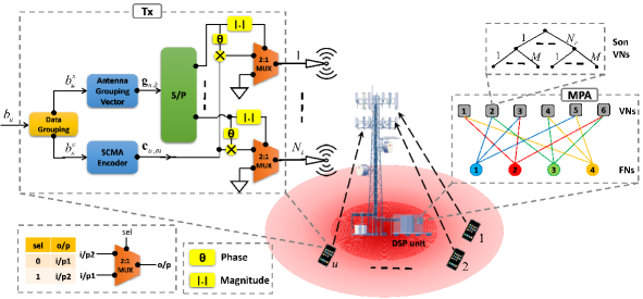
Fig. 1: Uplink RGSM-SCMA block diagram for the $u$-th user.

In this section, the RGSM-SCMA system is introduced. Assume that $R$ orthogonal resource elements (OREs), e.g., subcarriers, are overloaded with $U$ users (i.e., $U>R$); each user has a unique sparse codebook, $\mathbf{C}_{u}\in\mathbb{C}^{R\times M}$, $u=1,\ldots,U$, which contains $M$ codewords, $\mathbf{c}_{u,m}\in\mathbb{C}^{R\times 1}$, $m=1,\ldots,M$. $\mathbf{c}_{u,m}$ has $d_{v}$ non-zero codeword elements in the same positions for each codebook, and vary from one codebook to another. The number of the overlapped users per ORE, $d_{f}$, is fixed for $\forall R$. The SE for the $u$-th user is $\eta_{u}=\eta_{u}^{s}+\eta_{u}^{c}$ bit per channel use (bpcu), where $\eta_{u}^{s}$ and $\eta_{u}^{c}$ denote the spatial and code spectral efficiencies, respectively.

Consider that $N_{t}$ and $M$ are the number of transmit antennas used to deliver $\eta_{u}^{s}$ bpcu and the number of codewords used to deliver $\eta_{u}^{c}$ bpcu, respectively, for each user. It is assumed that the system parameters for all users are the same (i.e., same $N_{t}$, SEs and $M$). In the RGSM-SCMA system, $\eta_{u}^{s}=\log_{2}(N_{c})$ bpcu, where $N_{c}=2^{n_{c}}$ antenna combinations, $n_{c}=$$\left\lfloor\log_{2}\left(\begin{array}[]{c}N_{t}\\ N_{a}\end{array}\right)\right\rfloor$, with $\left\lfloor\cdot\right\rfloor$ as the floor operation, and $N_{a}<N_{t}$ is the number of active antennas at a time, while $\eta_{u}^{c}=\log_{2}(M)$ bpcu.

Fig. 1 shows the uplink scenario of the RGSM-SCMA system for the $u$-th user; the input $\mathbf{b}_{u}\in\mathbb{B}^{\eta_{u}}$ bits for the $u$-th user is divided into two parts: the first $\mathbf{b}_{u}^{s}\in\mathbb{B}^{\eta_{u}^{s}}$ bits represent the spatial symbol, while the last $\mathbf{b}_{u}^{c}\in\mathbb{B}^{\eta_{u}^{c}}$ bits represent the code symbol. The SCMA encoder block maps the $\mathbf{b}_{u}^{c}$ bits to its corresponding codeword $\mathbf{c}_{u,m}$ and delivers it to the input of all transmit antenna multiplexers. The antenna grouping vector block chooses the antenna grouping vector, $\mathbf{g}_{u,k}\in\mathbb{C}^{1\times N_{t}}$, $k\in\{1,\ldots,N_{c}\}$, according to the value of $\mathbf{b}_{u}^{s}$ from a predetermined lookup table (Table I is an example lookup table with $N_{t}=5$, $N_{a}=2$, $N_{c}=8$, and $\mathbf{b}_{u}^{s}=3$ bpcu). It should be noted that $\mathbf{g}_{u,k}$ has $N_{a}$ non-zero elements that correspond to the $N_{a}$ active antennas. The serial-to-parallel (S/P) block distributes the zero and non-zero elements of $\mathbf{g}_{u,k}$ at the same time, to the next stage. The magnitude of $\mathbf{g}_{u,k}$, $\left|\mathbf{g}_{u,k}\right|\in\mathbb{R}^{1\times N_{t}}$, is applied to the multiplexers’ selector pins, which allow the antennas corresponding to the non-zero elements to transmit $\mathbf{c}_{u,m}$ rotated with the associated rotation angle of $\mathbf{g}_{u,k}$. To ensure maximum distance between the successive angles, they should be equally spaced for each antenna. Thus, the rotation angles of the $n_{t}$-th antenna are

TABLE I: The RGSM-SCMA antenna grouping vector lookup table for $N_{t}=5$, $N_{a}=2$, $N_{c}=8$, and $\eta_{u}^{s}=3$ bpcu.

$\mathbf{b}_{u}^{s}$	$k$	$\mathbf{g}_{u.k}$
$000$	$1$	$[\begin{array}[]{ccccc}1&0&\,\,\,1&\hskip 14.22636pt0&\hskip 14.22636pt0\end{array}]$
$001$	$2$	$[\begin{array}[]{ccccc}\text{e}^{-j\frac{2\pi}{3}}&0&\,\,\,0&\hskip 14.22636pt1&\hskip 14.22636pt0\end{array}]$
$010$	$3$	$[\begin{array}[]{ccccc}\text{e}^{-j\frac{4\pi}{3}}&0&\,\,\,0&\hskip 14.22636pt0&\hskip 14.22636pt1\end{array}]$
$011$	$4$	$[\begin{array}[]{ccccc}0&\,\,\,1&\,\,\,\,\text{e}^{-j\frac{\pi}{2}}&\,\,\,\,\,\,\,\,\,0&\hskip 14.22636pt0\end{array}]$
$100$	$5$	$[\begin{array}[]{ccccc}0&\,\,\,\text{e}^{-j\frac{2\pi}{3}}&\,\,0&\,\text{e}^{-j\frac{2\pi}{3}}&\hskip 14.22636pt0\end{array}]$
$101$	$6$	$[\begin{array}[]{ccccc}0&\,\,\,\,\text{e}^{-j\frac{4\pi}{3}}&\,0&\,0&\text{e}^{-j\frac{2\pi}{3}}\end{array}]$
$110$	$7$	$[\begin{array}[]{ccccc}0&\,\,\,0&\,\,\,\,\,\,\text{e}^{-j\pi}&\text{e}^{-j\frac{4\pi}{3}}&\hskip 14.22636pt0\end{array}]$
$111$	$8$	$[\begin{array}[]{ccccc}0&\,\,\,\,\,0&\hskip 14.22636pt\text{e}^{-j\frac{3\pi}{2}}&\,\,\,\,\,\,0&\text{e}^{-j\frac{4\pi}{3}}\end{array}]$

$$\theta_{d,n_{t}}=\frac{-2\left(d-1\right)\pi}{a_{n_{t}}},\,\,\,n_{t}=1,\ldots,N_{t},\,\,d=1,\ldots,a_{n_{t}},$$ (1)

where $\theta_{d,n_{t}}$ denotes the rotation angle of the $d$-th occurrence of the $n_{t}$-th antenna, and $a_{n_{t}}$ is the number of times that the $n_{t}$-th antenna is activated for $\forall k$. For instance, in Table I, the third antenna (i.e., $n_{t}=3$) is activated 4 times (i.e., $a_{3}=4$) at $k=1,\,4,\,7$ and $8$. Then, $\theta_{1,3}$, $\theta_{2,3}$, $\theta_{3,3}$ and $\theta_{4,3}$ equal to $0$, $\frac{-\pi}{2}$, $-\pi$ and $\frac{-3\pi}{2}$, respectively.

At the receiver side, the noisy received signal for each ORE at the $n$-th receive antenna, $y_{n}^{r}$, is

$$y_{n}^{r}=\sum_{u\in\varLambda_{r}}\left(\mathbf{h}_{u,n}^{r}\mathbf{g}_{u,k}^{\text{T}}c_{u,m}^{r}\right)+n_{n}^{r},$$ (2)

where $\mathbf{h}_{u,n}^{r}\in\mathbb{C}^{1\times N_{t}}$ denotes the Rayleigh fading channel between the $N_{t}$ transmit antennas and $n$-th receive antenna of the $u$-th user for the $r$-th ORE, $c_{u,m}^{r}$ represents the $r$-th element of the $m$-th codeword for user $u$, $n_{n}^{r}\sim\mathcal{N}\left(0,\sigma^{2}\right)$ is the Gaussian noise at the $r$-th ORE of the $n$-th receive antenna with zero-mean and a variance of $\sigma^{2}$, and $\varLambda_{r}$ is the set of indices of the users that share the $r$-th ORE. The received signals vector, $\mathbf{y}_{n}$, for all OREs at the $n$-th receive antenna is

$$\mathbf{y}_{n}=\sum_{u=1}^{U}\left(\mathrm{diag}\left(\mathbf{h}_{u,n}\mathbf{g}_{u,k}^{\text{T}}\right)\mathbf{c}_{u,m}\right)+\mathbf{n}_{n},$$ (3)

where $\mathbf{y}_{n}\in\mathbb{C}^{R\times 1}=\left[y_{n}^{1},\ldots,y_{n}^{R}\right]^{\text{T}}$, $\mathbf{h}_{u,n}\in\mathbb{C}^{R\times N_{t}}=\left[\mathbf{h}_{u,n}^{1\,T},\ldots,\mathbf{h}_{u,n}^{R\,T}\right]^{\text{T}}$, $\mathbf{n}_{n}\in\mathbb{C}^{R\times 1}=\left[n_{n}^{1}\ldots n_{n}^{R}\right]^{\text{T}}$, and $\mathrm{diag}\left(\mathbf{h}_{u,n}\mathbf{g}_{u,k}^{\text{T}}\right)\in\mathbb{C}^{R\times R}$ is a diagonal matrix whose $r$-th diagonal element is $\mathbf{h}_{u,n}^{r}\mathbf{g}_{u,k}^{\text{T}}$.

IV RGSM-SCMA Signal Detection

In this section, the formulation of three decoders for the proposed RGSM-SCMA system is deduced, which are ML, MAP, and MPA decoders.

IV-A ML Decoder

The ML decoder performs an exhaustive search for all $\left(N_{c}M\right)^{U}$ possibilities to provide the optimum BER performance. The ML solution for $N_{r}$ receive antennas is

$\left\{\hat{\mathbf{C}},\hat{\mathbf{G}}\right\}=\underset{\begin{array}[]{c}j\in N_{c}^{U}\\ l\in M^{U}\end{array}}{\text{arg}\,\text{min}}$

$$\left\{\sum_{n=1}^{N_{r}}\left\|\mathbf{y}_{n}-\sum_{u=1}^{U}\left(\text{diag}\left(\mathbf{h}_{u,n}\mathbf{g}_{u,k(j)}^{\text{T}}\right)\mathbf{c}_{u,m(l)}\right)\right\|^{2}\right\}.$$ (4)

Here, $\hat{\mathbf{C}}\in\mathbb{C}^{R\times U}=\left[\hat{\mathbf{c}}_{1,m}\ldots\hat{\mathbf{c}}_{U,m}\right]$ denotes the estimated transmitted codewords for all users, with $\hat{\mathbf{c}}_{u,m}$ as the estimated transmitted codeword for the $u$-th user, and $m(l)$ represents the value of $m\in\left\{1,\ldots,M\right\}$ at the $l$-th antenna combination. $\hat{\mathbf{G}}\in\mathbb{C}^{U\times N_{t}}=\left[\hat{\mathbf{g}}_{1,k}\ldots\hat{\mathbf{g}}_{U,k}\right]$ denotes the estimated grouping vectors for all users, with $\hat{\mathbf{g}}_{u,k}$ as the estimated grouping vector for the $u$-th user, and $k(j)$ represents the value of $k\in\left\{1,\ldots,N_{c}\right\}$ at the $j$-th antenna combination.

IV-B MAP Decoder

Unlike the ML decoder, the MAP decoder estimates the pair of transmitted codeword and grouping vector, $\{\hat{\mathbf{c}}_{u,m},\hat{\mathbf{g}}_{u,k}\}$, for each user one-by-one by maximizing a posteriori probability of this pair given the received signal as

$$\left\{\hat{\mathbf{c}}_{u,m},\hat{\mathbf{g}}_{u,k}\right\}=\underset{\begin{array}[]{c}\hat{\mathbf{c}}_{u,m}\in\mathbf{C}_{u}\\ \hat{\mathbf{g}}_{u,k}\in\mathbf{G}_{u}\end{array}}{\text{arg}\,\text{max}}\left\{P\left(\{\hat{\mathbf{c}}_{u,m},\hat{\mathbf{g}}_{u,k}\}|\mathbf{y}_{n}\right)\right\}$$

$$=\underset{\begin{array}[]{c}\hat{\mathbf{c}}_{u,m}\in\mathbf{C}_{u}\\ \hat{\mathbf{g}}_{u,k}\in\mathbf{G}_{u}\end{array}}{\text{arg}\,\text{max}}\left\{P\left(\{\hat{\mathbf{c}}_{u,m},\hat{\mathbf{g}}_{u,k}\}\right)P\left(\mathbf{y}_{n}|\{\hat{\mathbf{c}}_{u,m},\hat{\mathbf{g}}_{u,k}\}\right)\right\}$$

$$=\underset{\begin{array}[]{c}\hat{\mathbf{c}}_{u,m}\in\mathbf{C}_{u}\\ \hat{\mathbf{g}}_{u,k}\in\mathbf{G}_{u}\end{array}}{\text{arg}\,\text{max}}\{\sum_{\begin{array}[]{c}\left.\mathbf{\exists}\right\backslash\{\hat{\mathbf{c}}_{u,m},\hat{\mathbf{g}}_{u,k}\}\\ \,\in\left.\mathbf{\Xi}\right\backslash\{\mathbf{C}_{u},\mathbf{G}_{u}\}\end{array}}P\left(\{\hat{\mathbf{c}}_{u,m},\hat{\mathbf{g}}_{u,k}\},\left.\mathbf{\exists}\right\backslash\{\hat{\mathbf{c}}_{u,m},\hat{\mathbf{g}}_{u,k}\}\right)$$

$$\hskip 56.9055pt\times P\left(\mathbf{y}_{n}|\{\hat{\mathbf{c}}_{u,m},\hat{\mathbf{g}}_{u,k}\},\left.\mathbf{\exists}\right\backslash\{\hat{\mathbf{c}}_{u,m},\hat{\mathbf{g}}_{u,k}\}\right)\},$$ (5)

where $\mathbf{\exists}=\left[\{\hat{\mathbf{c}}_{1,m},\hat{\mathbf{g}}_{1,k}\},\ldots,\{\hat{\mathbf{c}}_{U,m},\hat{\mathbf{g}}_{U,k}\}\right]$ represents one possible combination of the transmitted set of codewords and grouping vectors for all $U$ users, $\mathbf{\Xi}$ is the set containing all $\left(N_{c}M\right)^{U}$ possibilities of $\mathbf{\exists}$, $\left.\mathbf{\exists}\right\backslash\{\hat{\mathbf{c}}_{u,m},\hat{\mathbf{g}}_{u,k}\}$ denotes $\mathbf{\exists}$ except the set $\{\hat{\mathbf{c}}_{u,m},\hat{\mathbf{g}}_{u,k}\}$, and $\left.\mathbf{\Xi}\right\backslash\{\mathbf{C}_{u},\mathbf{G}_{u}\}$ denotes $\mathbf{\Xi}$ except $\{\mathbf{C}_{u},\mathbf{G}_{u}\}$. Note that the total probability theorem is applied to obtain the last line of (5). Since all elements of $\mathbf{y}_{n}$ are independent for all OREs and $N_{r}$ receive antennas, the conditional probability in the last term of (5) becomes

$$P\left(\mathbf{y}_{n}|\{\hat{\mathbf{c}}_{u,m},\hat{\mathbf{g}}_{u,k}\},\left.\mathbf{\exists}\right\backslash\{\hat{\mathbf{c}}_{u,m},\hat{\mathbf{g}}_{u,k}\}\right)=\prod_{n=1}^{N_{r}}\prod_{r\in\Omega_{u}}P\left(\mathbf{y}_{n}|\mathbf{\exists}(r)\right),$$ (6)

where $\Omega_{u}$ is the set of indices of the $d_{v}$ non-zero OREs for the $u$-th user, $\mathbf{\exists}(r)$ denotes one possible set of transmitted codewords and grouping vectors at the $r$-th ORE for the $d_{f}$ users that share the $r$-th ORE, and

$$P\left(\mathbf{y}_{n}|\mathbf{\exists}(r)\right)=\frac{1}{\sqrt{2\pi}\sigma}\text{exp}\left(-\frac{\left|y_{n}^{r}-\sum_{u\in\varLambda_{r}}\left(\mathbf{h}_{u,n}^{r}\mathbf{g}_{u,k}^{\text{T}}c_{u,m}^{r}\right)\right|^{2}}{2\sigma^{2}}\right).$$ (7)

IV-C MPA Decoder

TABLE II: The real operations of the MPA decoders for the SM-SCMA and RGSM-SCMA systems.

	SM-SCMA	RGSM-SCMA
Additions	$\begin{array}[]{c}Rd_{f}\left(N_{t}M\right)^{d_{f}}\left(2N_{r}(2d_{f}+1)-1\right)\\ +TRd_{f}\left(\left(N_{t}M\right)^{d_{f}}-1\right)\end{array}$	$\begin{array}[]{c}Rd_{f}\left(N_{c}M\right)^{d_{f}}\left(2N_{r}(2d_{f}+1)-1\right)\\ +TRd_{f}\left(\left(N_{c}M\right)^{d_{f}}-1\right)+2Ud_{v}N_{r}N_{c}\left(2N_{a}-1\right)\end{array}$
Multiplications	$\begin{array}[]{c}Rd_{f}\left(N_{t}M\right)^{d_{f}}\left(2N_{r}(2d_{f}+1)+Td_{f}+1\right)\\ +N_{t}M\left(d_{v}-1\right)\left(TRd_{f}+U\right)\end{array}$	$\begin{array}[]{c}Rd_{f}\left(N_{c}M\right)^{d_{f}}\left(2N_{r}(2d_{f}+1)+Td_{f}+1\right)\\ +N_{c}M\left(d_{v}-1\right)\left(TRd_{f}+U\right)+4Ud_{v}N_{r}N_{c}N_{a}\end{array}$

The MPA decoder provides an approximation to the MAP detector using the factor graph method, shown in Fig. 1. In the factor graph, the OREs and served users are represented as function nodes (FNs) and variable nodes (VNs), respectively. For each FN, all VNs that share this FN are connected. Note that each VN has $N_{c}M$ son VNs. The idea of the MPA is to iteratively update the probability of passing the messages from FNs to VNs and vice versa. After $T$ iterations, the MPA stops and detects the message which corresponds to the maximum joint probability. Note that the conventional MPA of the proposed RGSM-SCMA is modified to jointly estimate the antenna grouping vector and transmitted codeword.

To formulate the MPA, assume that $\mathcal{P}_{f_{r}\rightarrow v_{u}}^{(t)}(\{c_{u,m}^{r},\mathbf{g}_{u,k}\})$ and $\mathcal{P}_{v_{u}\rightarrow f_{r}}^{(t)}(\{c_{u,m}^{r},\mathbf{g}_{u,k}\})$ is the probability of passing the message $\{c_{u,m}^{r},\mathbf{g}_{u,k}\}$ from the $r$-th FN to the $u$-th VN and from the $u$-th VN to the $r$-th FN, respectively, at the $t$-th iteration, $t=1,\ldots,T$. First, all messages sent from VNs to FNs are assumed equiprobable at the first iteration; i.e.,

$$\mathcal{P}_{v_{u}\rightarrow f_{r}}^{(0)}\left(\{c_{u,m}^{r},\mathbf{g}_{u,k}\}\right)=\frac{1}{N_{c}M},\,\,\,\,\,\forall u,\,\,\forall r,\,\,\forall m,\,\,\forall k.$$ (8)

Now, $\mathcal{P}_{f_{r}\rightarrow v_{u}}^{(t+1)}(\{c_{u,m}^{r},\mathbf{g}_{u,k}\})$ can be written as

$$\mathcal{P}_{f_{r}\rightarrow v_{u}}^{(t+1)}\left(\{c_{u,m}^{r},\mathbf{g}_{u,k}\}\right)=\,\hskip 142.26378pt$$

$$\sum_{\mathbf{\exists}(i),i\in\left.\varLambda_{r}\right\backslash u}\left\{\prod_{n=1}^{N_{r}}\left(P\left(\mathbf{y}_{n}|\mathbf{\exists}(i),\mathbf{\exists}(u)=\{c_{u,m}^{r},\mathbf{g}_{u,k}\}\right)\right)\right.$$

$$\left.\times\prod_{i\in\left.\varLambda_{r}\right\backslash u}\mathcal{P}_{v_{i}\rightarrow f_{r}}^{(t)}\left(\mathbf{\exists}(i)\right)\right\},\,\,\,\,\,\forall m,\,\,\forall k,\,\,\forall r,\,\,u\in\varLambda_{r},$$ (9)

where $\left.\varLambda_{r}\right\backslash u$ denotes $\varLambda_{r}$ except the $u$-th user, and $P\left(\mathbf{y}_{n}|\mathbf{\exists}(i),\mathbf{\exists}(u)=\{c_{u,m}^{r},\mathbf{g}_{u,k}\}\right)$ is given in (7). Then, the probability of passing the messages from VNs to FNs is updated as

$$\mathcal{P}_{v_{u}\rightarrow f_{r}}^{(t+1)}\left(\{c_{u,m}^{r},\mathbf{g}_{u,k}\}\right)=\gamma_{u,r}^{(t+1)}\prod_{j\in\left.\Omega_{u}\right\backslash r}\mathcal{P}_{f_{j}\rightarrow v_{u}}^{(t+1)}\left(\{c_{u,m}^{r},\mathbf{g}_{u,k}\}\right),$$

$$\hskip 113.81102pt\forall m,\,\,\forall k,\,\,\forall u,\,\,r\in\Omega_{u},$$ (10)

where $\left.\Omega_{u}\right\backslash r$ denotes $\Omega_{u}$ except the $r$-th ORE, and $\gamma_{u,r}^{(t+1)}$ is the normalization factor, which is given by

$$\gamma_{u,r}^{(t+1)}=\left(\sum_{m=1}^{M}\sum_{k=1}^{N_{c}}\mathcal{P}_{v_{u}\rightarrow f_{r}}^{(t)}\left(\{c_{u,m}^{r},\mathbf{g}_{u,k}\}\right)\right)^{-1}.$$ (11)

After $T$ iterations, the estimated transmitted codeword and grouping vector are obtained as

$$\left\{\hat{\mathbf{c}}_{u,m},\hat{\mathbf{g}}_{u,k}\right\}=\underset{\begin{array}[]{c}m=1,\ldots,M\\ k=1,\ldots,N_{c}\end{array}}{\text{arg}\,\text{max}}\prod_{j\in\Omega_{u}}\mathcal{P}_{f_{j}\rightarrow v_{u}}^{(T)}\left(\{\mathbf{c}_{u,m},\mathbf{g}_{u,k}\}\right),\,\,\,\forall u.$$ (12)

IV-D MPA Complexity Analysis

In this subsection, the computational complexity of the MPA decoders for the SM-SCMA and RGSM-SCMA systems is deduced in terms of real additions and multiplications. Table II shows the complexity summary, calculated based on (8)-(12) and the factor graphs of both systems. At the same SE, it is shown from Table II that there is a negligible increase in the number of real multiplications and additions of the RGSM-SCMA by $4Ud_{v}N_{r}N_{c}N_{a}$ and $2Ud_{v}N_{r}N_{c}\left(2N_{a}-1\right)$, respectively. This increase is a result of combining the channel entries by the antenna grouping vectors before performing the MPA decoder, and is independent of the number of iterations. Thus, at the same SE, the decoding complexity of both systems is almost similar.

V Simulation Results

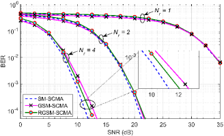
Fig. 2: BER performance comparison.

In this section, simulation is used to study the BER performance of the proposed RGSM-SCMA system, additionally in comparison with the SM-SCMA [12]. The effect of the rotation angles in (1) is shown, and we refer to the zero rotation angles version of the RGSM-SCMA as GSM-SCMA. The MPA decoder is considered for all systems. Furthermore, the Rayleigh fading channel is assumed to be perfectly known at the receiver. The required number of transmit antennas and decoding complexity comparisons between the proposed RGSM-SCMA and SM-SCMA are also provided. The system parameters for all systems are chosen as follows: $U=6$, $R=4$ and $M=4$.

Fig. 2 shows the BER performance comparison for $\eta_{u}^{s}=3$ bpcu ($N_{t}=8$ and $5$ for SM-SCMA and RGSM-SCMA, respectively), $N_{a}=2$ and $T=2$ in case of $N_{r}=1,\,2$, and $4$. As shown in this figure, the BER performance is almost the same in the case of $N_{r}=1$ and $2$. In the case of high signal-to-noise ratio (SNR) for $N_{r}=4$, the proposed RGSM-SCMA provides a better BER performance than the GSM-SCMA. Thus, using the rotation angles in (1) for the proposed RGSM-SCMA degrades the BER performance by only $0.6$ dB instead of $1.2$ dB SNR as in GSM-SCMA, when compared with SM-SCMA.

Fig. 3 shows the extra complexity (ExCo) of the RGSM-SCMA over SM-SCMA mentioned in Table II and given by: ExCo = (RGSM operations - SM operations) / SM operations, where operations can be either additions or multiplications. It can be seen from Fig. 3 that the ExCo is negligible (less than $0.05\%$) for both additions and multiplications, and decreases when $T$ or $\eta_{u}^{s}$ increase.

The RGSM-SCMA system provides significant savings in the number of transmit antennas, $N_{t}$, required to deliver the same $\eta_{u}^{s}$ of the SM-SCMA, as shown in Fig. 4. Note that $N_{a}=\{2,2,3,3,4,4,4,5,5\}$ is used to achieve $\eta_{u}^{s}=2:10$ bpcu. The RGSM-SCMA saves more in terms of $N_{t}$ when $\eta_{u}^{s}$ increases. For example, to deliver $\eta_{u}^{s}=7$ bpcu, the SM-SCMA requires $128$ transmit antennas, while the RGSM-SCMA requires only $10$ antennas.

Finally, the RGSM-SCMA provides a significant reduction in the number of transmit antennas with almost the same decoding complexity and a very slight deterioration in the BER performance to deliver the same SE of the SM-SCMA.

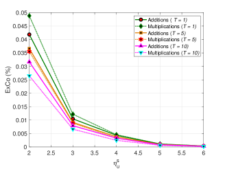
Fig. 3: Extra complexity comparison between SM-SCMA and RGSM-SCMA.

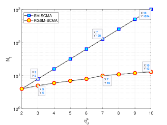
Fig. 4: $N_{t}$ comparison between SM-SCMA and RGSM-SCMA.

VI Conclusion

A low-cost SM-SCMA system has been proposed, which utilizes a reduced number of transmit antennas, referred to as RGSM-SCMA. The transmitter design, as well as the ML and MAP decoders have been introduced. Furthermore, the low-complexity MPA decoder has been revised and analyzed for the proposed RGSM-SCMA system. This delivers the same SE as SM-SCMA with a much lower number of required antennas, at the expense of less than $0.05\%$ increase in the decoding complexity and up to $0.6$ dB SNR degradation in the BER performance.

References

• [1] M. Mohammadkarimi, M. A. Raza, and O. A. Dobre, β€œSignature-based nonorthogonal massive multiple access for future wireless networks: Uplink massive connectivity for machine-type communications,” IEEE Veh. Technol. Mag., vol. 13, no. 4, pp. 40–50, Dec. 2018.
• [2] S. M. R. Islam, N. Avazov, O. A. Dobre, and K. S. Kwak, β€œPower-domain non-orthogonal multiple access (NOMA) in 5G systems: Potentials and challenges,” IEEE Commun. Surv. Tuts., vol. 19, no. 2, pp. 721-742, Oct. 2016.
• [3] Z. Ding et al., β€œA survey on non-orthogonal multiple access for 5G networks: Research challenges and future trends,” IEEE J. Sel. Areas Commun., vol. 35, no. 10, pp. 2181 –2195, Oct. 2017.
• [4] H. Nikopour and H. Baligh, β€œSparse code multiple access,” in Proc. IEEE Int. Symposium on Personal Indoor and Mobile Radio Commun. (PIMRC), Sep. 2013, pp. 332–336.
• [5] M. Taherzadeh et al., β€œSCMA codebook design,” in Proc. IEEE Veh. Technol. Conf. (VTC Fall), Sep. 2014, pp. 1–5.
• [6] H. Mu, Z. Ma, M. Alhaji, P. Fan, and D. Chen, β€œA fixed low complexity message pass algorithm detector for up-link SCMA system,” IEEE Wireless Commun. Lett., vol. 4, no. 6, pp. 585–588, Dec. 2015.
• [7] R. Y. Mesleh et al., β€œSpatial modulation,” IEEE Trans. Veh. Technol., vol. 57, no. 4, pp. 2228–2241, Jul. 2008.
• [8] E. Basar, β€œIndex modulation techniques for 5G wireless networks,” IEEE Commun. Mag., vol. 54, no. 7, pp. 168–175, Jul. 2016.
• [9] A. Younis, N. Serafimovski, R. Mesleh, and H. Haas, β€œGeneralised spatial modulation,” in Proc. Forty Fourth Asilomar Conf. Signals, Syst., Comput. (ASILOMAR), Nov. 2010, pp. 1498–1502.
• [10] C. Zhong, X. Hu, X. Chen, D. W. Ng, and Z. Zhang, β€œSpatial modulation assisted multi-antenna non-orthogonal multiple access”, IEEE Wireless Commun. Lett., vol. 25, no. 2, pp. 61-67, Apr. 2018.
• [11] Y. Liu, L. L. Yang, and L. Hanzo, β€œSpatial modulation aided sparse code division multiple access,” IEEE Trans. Wireless Commun., vol. 17, no. 3, pp. 1474–1487, Mar. 2018.
• [12] Z. Pan, J. Luo, J. Lei, L. Wen, and C. Tang, β€œUplink spatial modulation SCMA system,” IEEE Commun. Lett., vol. 23, no. 1, pp. 184-187, Jan. 2019.
• [13] I. Al-Nahhal, O. A. Dobre, and S. Ikki, β€œQuadrature spatial modulation decoding complexity: Study and reduction,” IEEE Wireless Commun. Lett., vol. 6, pp. 378-381, Jun. 2017.
• [14] I. Al-Nahhal, O. A. Dobre, and S. Ikki, β€œLow complexity decoders for spatial and quadrature spatial modulations,” in Proc. IEEE Veh. Technol. Conf. (VTC-Spring), 2018, pp. 1–5.
• [15] I. Al-Nahhal, E. Basar, O. A. Dobre, and S. Ikki, β€œOptimum low-complexity decoder for spatial modulation,” Accepted in IEEE J. Sel. Areas Commun., 2019.