A Fast, Accurate, and Separable Method for Fitting a Gaussian Function

The Gaussian function (GF) is widely used to explain the behavior or statistical distribution of many natural phenomena as well as industrial processes in different disciplines of engineering and applied science. For example, the GF can be used to model an approximation of the Airy disk in image processing, laser heat source in laser transmission welding [1], practical microscopic applications [2], and fluorescence dispersion in flow cytometric DNA histograms [3]. In applied sciences, the noise that corrupts the signal can be modeled by the Gaussian distribution according to the central limit theorem. Thus, by fitting the GF, the corresponding process/phenomena behavior can be well interpreted.

This article introduces a novel fast, accurate, and separable algorithm for estimating the GF parameters to fit observed data points. A simple mathematical trick can be used to calculate the area under the GF in two different ways. Then, by equating these two areas, the GF parameters can be easily obtained from the observed data.

Gaussian Function Fitting Approaches

A GF has a symmetrical bell-shape around its center, with a width that smoothly decreases as it moves away from its center on the $x$-axis. The mathematical form of the GF is

$$y(x)=Ae^{-\frac{(x-\mu)^{2}}{2\sigma^{2}}},$$ (1)

with three shape-controlling parameters, $A$, $\mu$ and $\sigma$, where $A$ is the maximum height (amplitude) that can be achieved on the $y$-axis, $\mu$ is the curve-center (mean) on the $x$-axis, and $\sigma$ is the standard deviation (SD) which controls the width of the curve along the $x$-axis. The aim of this article is to present a new method for the accurate estimation of these three parameters. The difficulty of this lies in estimating the three shape-controlling parameters ($A$, $\mu$ and $\sigma$) from observations, that are generally noisy, by solving an over-determined nonlinear system of equations.

The standard solutions for fitting the GF parameters from noisy observed data are obtained by one of the following two approaches:

1. Solving the problem as a nonlinear system of equations using one of the least-squares optimization algorithms. This solution employs an iterative procedure such as the Newton-Raphson algorithm [4]. The drawbacks of this approach are the iterative procedure, which may not converge to the true solution, as well as its high cost from the computational complexity perspective.

2. Solving the problem as a linear system of equations based on the fact that the GF is an exponential of a quadratic function. By taking the natural logarithm of the observed data, the problem can be solved in polynomial time as a $3\times 3$ linear system of equations. Two traditional algorithms have been proposed in this context: Caruana’s algorithm [5] and Guo’s algorithm [6]. Furthermore, instead of taking the natural logarithm, the partial derivative is used in Roonizi’s algorithm [7].

In this article, we will consider only the second approach, which is more suitable for most scientific applications, due to its simplicity and avoidance of the drawbacks of the first approach. Let us start with a brief introduction of the existing three algorithms for the second approach.

Caruana’s Algorithm

Caruana’s algorithm exploits the fact that the GF is an exponential of a quadratic function and transforms it into a linear form by taking the natural logarithm of (1) to obtain

$$\text{ln}(y)=\text{ln}(A)+\frac{-(x-\mu)^{2}}{2\sigma^{2}}=\text{ln}(A)-\frac{\mu^{2}}{2\sigma^{2}}+\frac{2\mu x}{2\sigma^{2}}-\frac{x^{2}}{2\sigma^{2}}=a+bx+cx^{2},$$ (2)

where $a=\text{ln}(A)-\mu^{2}/\left(2\sigma^{2}\right)$, $b=\mu/\sigma^{2}$ and $c=-1/\left(2\sigma^{2}\right)$. Accordingly, the unknowns become $a$, $b$ and $c$ in the linear equation (2) instead of $A$, $\mu$ and $\sigma$ in the nonlinear equation (1). Next, if the observations $y$ are noisy, then they can be modeled as $\hat{y}=y+w$; each contains the ideal data point, $y$, that is corrupted by the noise, $w$ with SD of $\sigma_{w}$. Note that in (2), we consider only the observations that have values above zero.

Once we have an over-determined linear system, the unknowns can be estimated using the least-squares method. Caruana’s algorithm estimates the three unknowns ($a$, $b$ and $c$) in (2) using the least-squares method by forming the error function, $\varepsilon$, for (2) as

$$\varepsilon=\text{ln}(\hat{y})-\text{ln}(y)=\text{ln}(\hat{y})-(a+bx+cx^{2}).$$ (3)

Then, by differentiating the sum of $\varepsilon^{2}$ with respect to $a$, $b$ and $c$ and equating the results to zero, we obtain three equations, which represent the following linear system

$$\left[\begin{array}[]{ccc}N&\sum x_{n}&\sum x_{n}^{2}\\ \sum x_{n}&\sum x_{n}^{2}&\sum x_{n}^{3}\\ \sum x_{n}^{2}&\sum x_{n}^{3}&\sum x_{n}^{4}\end{array}\right]\left[\begin{array}[]{c}a\\ b\\ c\end{array}\right]=\left[\begin{array}[]{c}\sum\text{ln}(\hat{y}_{n})\\ \sum x_{n}\text{ln}(\hat{y}_{n})\\ \sum x_{n}^{2}\text{ln}(\hat{y}_{n})\end{array}\right],$$ (4)

where $N$ is the number of observed data points and $\sum$ denotes $\sum_{n=1}^{N}$. In this case, the parameters $a$, $b$ and $c$ can be determined simply by solving (4) as a determined linear system of equations. Subsequently, the original parameters of the GF are determined as

$$A=e^{a-\frac{b^{2}}{4c}},\,\,\,\,\,\,\,\mu=\frac{-b}{2c},\,\,\,\,\,\,\,\sigma=\sqrt{\frac{-1}{2c}}.$$ (5)

The weighted least-squares method is the second candidate method to estimate the unknowns, and it is expected to have a better accuracy in estimation rather than the least-squares method.

Guo’s Algorithm

Guo’s algorithm is a modified version of the Caruana’s algorithm, which finds the unknowns $a$, $b$ and $c$ in (2) using the weighted least-squares method. It uses the noisy observed data, $\hat{y}$, to weight the error function in (3). Therefore, the error equation in (3) becomes $\delta=\hat{y}\varepsilon=\hat{y}[\text{ln}(\hat{y})-(a+bx+cx^{2})]$, and the linear system of equations in (4) becomes

$$\left[\begin{array}[]{ccc}\sum\hat{y}_{n}^{2}&\sum x_{n}\hat{y}_{n}^{2}&\sum x_{n}^{2}\hat{y}_{n}^{2}\\ \sum x_{n}\hat{y}_{n}^{2}&\sum x_{n}^{2}\hat{y}_{n}^{2}&\sum x_{n}^{3}\hat{y}_{n}^{2}\\ \sum x_{n}^{2}\hat{y}_{n}^{2}&\sum x_{n}^{3}\hat{y}_{n}^{2}&\sum x_{n}^{4}\hat{y}_{n}^{2}\end{array}\right]\left[\begin{array}[]{c}a\\ b\\ c\end{array}\right]=\left[\begin{array}[]{c}\sum\hat{y}_{n}^{2}\text{ln}(\hat{y}_{n})\\ \sum x_{n}\hat{y}_{n}^{2}\text{ln}(\hat{y}_{n})\\ \sum x_{n}^{2}\hat{y}_{n}^{2}\text{ln}(\hat{y}_{n})\end{array}\right].$$ (6)

Moreover, the values of $A$, $\mu$ and $\sigma$ can be computed from (5).

One of the problems that affects the estimation accuracy is the long tail GF. This is experienced when the number of small values in the observed data is large compared to the observed data length, $N$, which means that a large noise exists in those observations. Thus, an iterative procedure is required to improve the estimation accuracy.

Guo’s Algorithm with Iterative Procedure

The estimation accuracy of the Guo’s algorithm deteriorates for a long tail GF. In order to increase the accuracy of fitting the long tail Gaussian parameters, an iterative procedure for (6) is given as

$$\left[\begin{array}[]{ccc}\sum\hat{y}_{n,(k-1)}^{2}&\sum x_{n}\hat{y}_{n,(k-1)}^{2}&\sum x_{n}^{2}\hat{y}_{n,(k-1)}^{2}\\ \sum x_{n}\hat{y}_{n,(k-1)}^{2}&\sum x_{n}^{2}\hat{y}_{n,(k-1)}^{2}&\sum x_{n}^{3}\hat{y}_{n,(k-1)}^{2}\\ \sum x_{n}^{2}\hat{y}_{n,(k-1)}^{2}&\sum x_{n}^{3}\hat{y}_{n,(k-1)}^{2}&\sum x_{n}^{4}\hat{y}_{n,(k-1)}^{2}\end{array}\right]\left[\begin{array}[]{c}a_{(k)}\\ b_{(k)}\\ c_{(k)}\end{array}\right]=\left[\begin{array}[]{c}\sum\hat{y}_{n,(k-1)}^{2}\text{ln}(\hat{y}_{n})\\ \sum x_{n}\hat{y}_{n,(k-1)}^{2}\text{ln}(\hat{y}_{n})\\ \sum x_{n}^{2}\hat{y}_{n,(k-1)}^{2}\text{ln}(\hat{y}_{n})\end{array}\right],$$ (7)

where $\hat{y}_{n,(k)}=\hat{y}_{n}$ for $k=0$ and $\hat{y}_{n,(k)}=e^{a_{(k)}+b_{(k)}x_{n}+c_{(k)}x_{n}^{2}}$ for $k>0$, with the parenthesized subscripts denoting the indices of iteration.

Roonizi’s Algorithm

Roonizi’s algorithm is designed to fit the GF riding on a polynomial background. It can be utilized to fit a GF by taking the partial derivative of (1), and then taking the integral of the result to obtain

$$y(x)=\beta_{1}\phi_{1}(x)+\beta_{2}\phi_{2}(x),$$ (8)

where $\beta_{1}=-1/\sigma^{2}$, $\beta_{2}=\mu/\sigma^{2}$, and

$$\phi_{1}(x)=\int_{-\infty}^{x}u\,y(u)\,\,du,\,\,\,\,\,\,\,\,\phi_{2}(x)=\int_{-\infty}^{x}y(u)\,\,du.$$ (9)

Similar to the steps in Caruana’s and Guo’s algorithms, to obtain the linear system of equations, the error of (8) becomes $\zeta=\hat{y}-(\beta_{1}\phi_{1}(x)+\beta_{2}\phi_{2}(x))$, and a linear system of equations results as

$$\left[\begin{array}[]{cc}\sum\left|\phi_{1}(x_{n})\right|^{2}&\sum\phi_{1}(x_{n})\phi_{2}(x_{n})\\ \sum\phi_{1}(x_{n})\phi_{2}(x_{n})&\sum\left|\phi_{2}(x_{n})\right|^{2}\end{array}\right]\left[\begin{array}[]{c}\beta_{1}\\ \beta_{2}\end{array}\right]=\left[\begin{array}[]{c}\sum\phi_{1}(x_{n})\hat{y}_{n}\\ \sum\phi_{2}(x_{n})\hat{y}_{n}\end{array}\right].$$ (10)

By solving (10) in terms of $\beta_{1}$ and $\beta_{2}$, the estimated $\hat{\mu}$ and $\hat{\sigma}$ of the GF can be calculated as

$$\hat{\sigma}=\sqrt{\frac{-1}{\beta_{1}}},\,\,\,\,\,\,\,\,\,\hat{\mu}=\frac{-\beta_{2}}{\beta_{1}}.$$ (11)

Finally, using $\hat{\mu}$ and $\hat{\sigma}$ from (11), the estimated $\hat{A}$ of the GF can be calculated as

$$\hat{A}=\frac{\sum\left(\hat{y}_{n}\,\text{exp}\left(\frac{-(x_{n}-\hat{\mu})^{2}}{2\hat{\sigma}^{2}}\right)\right)}{\sum\text{exp}\left(\frac{-(x_{n}-\hat{\mu})^{2}}{2\hat{\sigma}^{2}}\right)}.$$ (12)

Note that the Roonizi’s algorithm has no iterative procedure to increase the accuracy of fitting long tail GF parameters.

Motivation

It is seen that Guo’s and Roonizi’s algorithms have better estimation accuracy than Caruana’s algorithm, while their computational complexity burden is comparable. Moreover, the three algorithms dependently estimate the GF parameters ($A$, $\mu$ and $\sigma$). This means that in some applications that require the estimation of only one parameter, the fitting algorithm may require unnecessary parameters to be estimated as well. Therefore, there is a need for a new method which provides better estimation accuracy with an efficient computational complexity, as well as the capability for a separable parameter estimation.

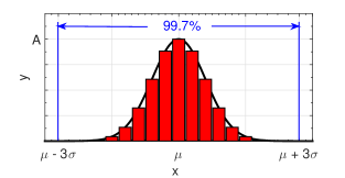
Figure 1: A Gaussian function.

Proposed Algorithm

In this article, we propose a novel computationally efficient (i.e., fast), accurate, and separable (FAS) algorithm for a GF that accurately fits the observed data. The basic idea of the proposed FAS algorithm is to find a direct formula for the SD (i.e., $\sigma$) parameter from the noisy observed data, and then, the amplitude $A$ and mean $\mu$ can be determined using the weighted least-squares method for only two unknowns.

Derivation of the Standard Deviation Formula

To derive an approximation formula for the SD, a simple mathematical trick will be used. For $N$ observations that represent the GF, as shown in Figure 1, the area under the GF can be divided into thin vertical rectangles with a width of $\Delta x_{n}$, where $\Delta x_{n}$ is the $n$-th step size of two successive observation points on the $x$-axis. Therefore, the total area under the GF, $\Lambda$, is numerically calculated as the summation of the areas of the vertical rectangles:

$$\Lambda\approx\sum_{n=1}^{N}\Delta x_{n}\hat{y}_{n}.$$ (13)

Note that (13) reflects at least $99.7\%$ of the GF area in case of an available observation width greater than $\mu\pm 3\sigma$. Now, let us calculate the area under the GF using a different method. From the GF and $Q$-function properties, the total area under the GF is given as

$$\Lambda=\intop_{-\infty}^{\infty}Ae^{-\frac{(x-\mu)^{2}}{2\sigma^{2}}}dx=A\sigma\sqrt{2\pi}.$$ (14)

Equating (13) and (14), and replacing the amplitude $A$ by the maximum value of the observed data, $\hat{y}_{\text{max}}$, the estimated $\sigma$ is obtained as

$$\hat{\sigma}=\frac{\sum_{n=1}^{N}\Delta x_{n}\hat{y}_{n}}{\sqrt{2\pi}\hat{y}_{\text{max}}}.$$ (15)

Thus, in certain applications which require the estimate of the SD of the GF, the FAS algorithm directly outputs this estimate, without estimating the other two parameters. This is referred to as the separable property of the FAS algorithm.

Error Analysis

To study the error of (15), first let us discuss the systematic error resulting from equating (13) and (14). This error becomes notable when a small portion of the GF is sampled, and it is from approximating the GF curve by rectangles (as in Figure 1). Based on extensive testing of the algorithm with varying parameters, as discussed further below, the systematic error can be considered negligible when $W>6$ and the observation samples are dense enough (e.g., $\frac{N}{W}>10$), where $W$ is the ratio of the SD to the observation width on the $x$-axis (i.e., the observation width equals $W\sigma$, or equivalently, it varies from $\mu-\frac{W}{2}\sigma$ to $\mu+\frac{W}{2}\sigma$).

To calculate the relative error in the numerator in (15), let the numerator equal $\sqrt{2\pi}A\sigma+\Delta x\sum_{n=1}^{N}w_{n}$, where $\sqrt{2\pi}A\sigma$ represents the actual area of the GF and $\Delta x\sum_{n=1}^{N}w_{n}$ is normally distributed with its SD being $\sqrt{N}\sigma_{w}\Delta x=\sqrt{N}\sigma_{w}\frac{W\sigma}{N}$. For simplicity of analysis, $\Delta x$ is considered to be fixed for all observations. The relative error of the numerator, $\alpha_{N}$, can be written as

$$\alpha_{N}\approx k_{1}\frac{\sigma_{w}W}{\sqrt{2\pi}A\sqrt{N}}=k_{1}\frac{W}{\text{snr}\sqrt{2\pi N}},$$ (16)

where $k_{1}$ is a constant value which can be considered $2$ for the $95.5\%$ confidence interval, and $\text{snr}=A/\sigma_{w}$ is the signal-to-noise ratio.

For the denominator, let us assume that it equals $\sqrt{2\pi}(A\pm\Delta A)$, where $\Delta A$ is the maximum of the normally distributed noise samples with SD of $\sigma_{w}$. The relative error of the denominator in (15), $\alpha_{D}$, can be written as

$$\alpha_{D}\approx\frac{k_{2}\sigma_{w}}{A}=\frac{k_{2}}{\text{snr}},$$ (17)

where $k_{2}$ is a constant whose value can be assumed to be $3$. Hence, the total relative error in (15), $\alpha$, can be approximated using a Taylor series as

$$\alpha\approx\alpha_{N}+\alpha_{D}=\frac{1}{\text{snr}}\left(k_{1}\frac{W}{\sqrt{2\pi N}}+k_{2}\right).$$ (18)

It is worth noting that if the samples are dense enough (i.e., large enough $N/W$) and for high snr, a reduced relative error can be attained.

Estimates of the Remaining Two Parameters

To estimate the remaining two parameters $A$ and $\mu$ using $\hat{\sigma}$ estimated from (15), we can differentiate the sum of $\delta^{2}$ with respect to $a$ and $b$ and then equate the results to zero (i.e., using the same steps as in Guo’s algorithm). The resulting linear system of equations becomes

$$\left[\begin{array}[]{cc}\sum\hat{y}_{n}^{2}&\sum x_{n}\hat{y}_{n}^{2}\\ \sum x_{n}\hat{y}_{n}^{2}&\sum x_{n}^{2}\hat{y}_{n}^{2}\end{array}\right]\left[\begin{array}[]{c}a\\ b\end{array}\right]=\left[\begin{array}[]{c}\sum\hat{y}_{n}^{2}\text{ln}(\hat{y}_{n})-c\sum x_{n}^{2}\hat{y}_{n}^{2}\\ \sum x_{n}\hat{y}_{n}^{2}\text{ln}(\hat{y}_{n})-c\sum x_{n}^{3}\hat{y}_{n}^{2}\end{array}\right],$$ (19)

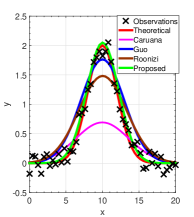
(a) ${\normalcolor N=50}$

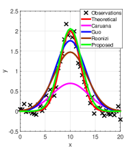
(b) $N=40$

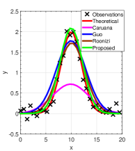
(c) $N=30$

Figure 2: Results of different algorithms for fitting the GF with $A=2$, $\sigma=2$ and $\mu=10$ in the presence of observation noise with $\sigma_{w}=0.1$ (i.e., snr = 10).

where $c=-1/\left(2\hat{\sigma}^{2}\right)$ and $\hat{\sigma}$ is the estimated SD, which is calculated from (15). Therefore, the values of $a$ and $b$ are obtained by solving the $2\times 2$ linear system in (19); then, the original parameters $A$ and $\mu$ can be calculated from (5).

Figure 2 shows the superiority of the proposed FAS algorithm over the traditional algorithms in the presence of a noise with SD $\sigma_{w}=0.1$ for different values of $N$; the proposed algorithm provides the best fit to the observed data points compared to the other fitting algorithms for all values of $N$. It is seen from Figure 2 that $\hat{y}_{\text{max}}$ is obviously different from the actual amplitude $A$. However, $\hat{\sigma}$ from (15) provides reasonable results using $\hat{y}_{\text{max}}$ even if a small number of observation points are available as in Figure 2(c).

Since the FAS algorithm provides poorer accuracy in fitting long tail GF parameters, an iterative procedure is required to improve the fitting accuracy.

FAS Algorithm with Iterative Procedure

For the long tail GF, we propose an iterative algorithm that improves the fitting accuracy of the FAS algorithm. The recursive version of (19) is given as

$$\left[\begin{array}[]{cc}\sum\hat{y}_{n,(k-1)}^{2}&\sum x_{n}\hat{y}_{n,(k-1)}^{2}\\ \sum x_{n}\hat{y}_{n,(k-1)}^{2}&\sum x_{n}^{2}\hat{y}_{n,(k-1)}^{2}\end{array}\right]\left[\begin{array}[]{c}a_{(k)}\\ b_{(k)}\end{array}\right]=\left[\begin{array}[]{c}\sum\hat{y}_{n,(k-1)}^{2}\text{ln}(\hat{y}_{n})-c\sum x_{n}^{2}\hat{y}_{n,(k-1)}^{2}\\ \sum x_{n}\hat{y}_{n,(k-1)}^{2}\text{ln}(\hat{y}_{n})-c\sum x_{n}^{3}\hat{y}_{n,(k-1)}^{2}\end{array}\right],$$ (20)

where $\hat{y}_{n,(k)}=\hat{y}_{n}$ for $k=0$ and $\hat{y}_{n,(k)}=e^{a_{(k)}+b_{(k)}x_{n}+cx_{n}^{2}}$ for $k>0$, and $\hat{\sigma}$ is estimated from (15) only once. This means that (15) can provide accurate results in fitting the long tail GF without iteration, while the other two parameters still need to be estimated through iterations. However, after a few iterations, $\hat{\sigma}$ can be further improved by including an updated SD from (15) in the iterations, using $A$ obtained by (20).

Figure 3 shows results of the iterative Guo and proposed FAS algorithms for fitting a long tail GF with $N=200$, $A=1$, $\sigma=2$ and $\sigma_{w}=0.1$ for $\mu=18$ and $19$, respectively. As we can see from the figure, the number of iterations required for the FAS algorithm to fit the long tail GF is lower than that of Guo’s algorithm. For example, in Figure 3(a), the FAS algorithm needs only 3 iterations to fit the observation; however, the Guo algorithm provides poor fitting for the same number of iterations. Note that, from Figure 3(b), the longer the tail of the GF, the more iterations that are needed (i.e., 6 iterations are needed instead of 3 to provide a good fitting to the longer tail GF). It is worthy of noting that in the presence of large noise and having a small portion of the GF, the iterative procedure of the proposed algorithm can nicely fit the GF only after a few iterations.

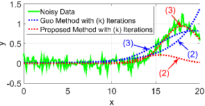
(a) $\mu=18$

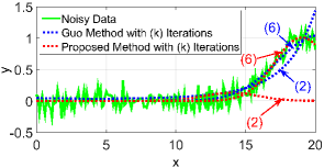
(b) $\mu=19$

Figure 3: Results of the proposed FAS iterative algorithm in comparison with Guo’s algorithm for fitting the GF of $N=200$, $A=1$, $\sigma=2$ and $\sigma_{w}=0.1$ (i.e., snr = 10).

Accuracy Comparison

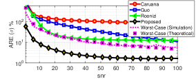
(a) $W=12$ and $N=30$.

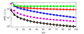
(b) $W=12$ and $N=200$.

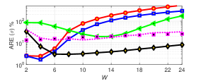
(c) snr = 25 and $N=30$.

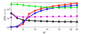
(d) snr = 25 and $N=200$.

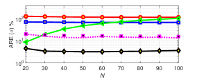
(e) $W=12$ and snr = 25.

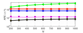
(f) $W=12$ and snr = 25.

Figure 4: ARE% of $\sigma$ estimated from different fitting algorithms.

In this section, Monte Carlo simulation results for at least $10^{4}$ simulated trials are considered to compare the average absolute relative error (ARE) of the fitting accuracy for the SD estimated using (15) and by the traditional algorithms. The ARE percentile of the SD is given as $\text{ARE\%}(\sigma)=\frac{\left|\hat{\sigma}-\sigma\right|}{\sigma}\times 100\%$, where $\left|\cdotp\right|$ denotes the absolute value and $\sigma$ is the true SD. The GF parameters used for this simulation are $A=1$, $\mu=10$ and $\sigma=2$. As demonstrated by the total relative error estimated in (18), three parameters can be used for assessing the accuracy of estimation (i.e., snr, $W$ and $N$).

For the evaluation of the estimation accuracy, we calculate the average $\text{ARE\%}(\sigma)$, where one of the three parameters is varying while the other two parameters are kept fixed. Figure 4 shows such results, where the SD is estimated using the proposed FAS algorithm in comparison with the three previously presented traditional algorithms. In Figures 4(a) and (b), $W=12$ and the snr varies from 1 to 100 for $N=30$ and $N=200$, respectively. Figures 4(c) and (d) depict the effect of $W$, which varies from $2$ to $24$, for $N=30$ and $N=200$, respectively, in the case of snr = 25 (i.e., $\sigma_{w}=0.04$). Figures 4(e) and (f) show the effect of $N$, which varies from $20$ to $100$ and from 200 to 1000, respectively, with $W=12$ and snr = 25. It is obvious from these figures that the SD estimated from (15) has the lowest ARE% in all cases, except for $W<6$ when Guo’s algorithm is the best. This is called the accurate property of the FAS algorithm. In many practical applications, an adequate portion of the GF (i.e., $W\geq 6$) is sampled with more than 200 observation points (i.e., $N\geq 200$). It is worth noting that Roonizi’s algorithm is more general than the rest of the techniques since it can also fit a Gaussian riding on a polynomial background. This might explain its poorer performance in comparison to the other algorithms that fit a sole GF as described by (1).

The plots in Figure 4 also depict the worst case ARE% of the proposed algorithm. The simulated worst-case ARE% represents the maximum ARE% that occurs during the $10^{4}$ simulated trials, which is compared to (18) with $k_{1}=2$ and $k_{2}=3$ to show the accuracy of our derived error estimated in (18). Note that the probability of such a worst-case error is very low. Notably, the worst-case theoretical and simulated ARE% match, except when $W<6$ due to the considerable systematic error. It is worth mentioning that the superiority of the proposed algorithm versus the traditional ones holds for the worse case ARE% as well; however, for the clarity of the plots in Figure 4, curves corresponding to the latter algorithms were not included. As shown in Fig. 4(f), after a particular value of $N$, the error of the denominator in (15) becomes dominant. As $N$ increases, there will be many samples around the peak of the GF, and the ARE% of the proposed algorithm slightly increases when $N$ increases, finally approaching the worst case scenario.

Complexity Comparison

We address the computational complexity comparison between the Guo, Roonizi and proposed FAS algorithms, in terms of the number of additions and multiplications required to complete the fitting procedure. We assume that subtraction and division operations are equivalent in complexity to addition and multiplication operations, respectively. It should be noted that solving an $n\times n$ linear system of equations using Gauss elimination requires $\left(2n^{3}+3n^{2}-5n\right)/6$ additions and $\left(n^{3}+3n^{2}-n\right)/3$ multiplications [8]. Therefore, the total number of additions (Add) and multiplications (Mul) for the Guo, Roonizi and FAS algorithms are given as:

$$\text{Ad}\text{d}^{(\text{Guo})}=N(A_{\text{ln}}+8)+3,\,\,\,\,\,\text{Mu}\text{l}^{(\text{Guo})}=N(M_{\text{ln}}+11)+17,$$ (21)

$$\text{Ad}\text{d}^{(\text{Roonizi})}=N^{2}+8N+NA_{\text{exp}}-5,\,\,\,\,\,\text{Mu}\text{l}^{(\text{Roonizi})}=0.5N^{2}+9.5N+NM_{\text{exp}}+9,$$ (22)

$${\normalcolor{\color[rgb]{0,0,1}{\normalcolor\text{Ad}\text{d}^{(\text{FAS})}=N(A_{\text{ln}}+8)-3,\,\,\,\,\,\text{Mu}\text{l}^{(\text{FAS})}=N(M_{\text{ln}}+10)+12,}}}$$ (23)

where $A_{\text{ln}}$ and $M_{\text{ln}}$ represent the number of additions and multiplications required to calculate the natural logarithm, respectively, while $A_{\text{exp}}$ and $M_{\text{exp}}$ represent the number of additions and multiplications required to calculate the natural exponential in (12), respectively. Note that the term of $N^{2}$ in (22) comes from the calculation of $\phi_{1}(x)$ in (9), which requires an accumulated numerical integration of $(u\,y(u))$ from the first observation point to the current value of $x$ for all $N$ observations.

It can be seen from (21)-(23) that the proposed algorithm requires fewer additions and multiplications when compared with Guo’s and Roonizi’s algorithms. Assuming $A_{\text{ln}}=A_{\text{exp}}$ and $M_{\text{ln}}=M_{\text{exp}}$, the proposed algorithm saves six additions and $\mathcal{O}\left(N\right)$ multiplications over the Guo’s algorithm, while it saves $\mathcal{O}(N^{2})$ additions and multiplications over the Roonizi’s algorithm. This is referred to as the fast property of the proposed FAS algorithm.

Conclusion

This article has proposed a simple approximation expression for the SD of a GF to fit a set of noisy observed data points. This expression results from a simple mathematical trick, which is based on the equality between the area under the GF calculated numerically and based on the $Q$-function properties. Then, the amplitude and mean of the GF can be calculated using the weighted least-squares method. Through comprehensive simulations and mathematical analysis, it has been shown that the proposed algorithm is not only faster than the Guo and Roonizi algorithms, but also provides better estimation accuracy when an adequate interval of the GF is sampled. Additionally, an iterative procedure is proposed, which is suitable to fit the GF when the observed data points are contaminated with substantial noise as in the long tail GF case. It has been shown by extensive computer simulations that the proposed iterative algorithm fits the GF faster than the iterative Guo algorithm. The proposed algorithm would be useful for several applications such as Airy disk approximation, laser transmission welding, fluorescence dispersion, and many digital signal processing applications.

Authors

Ibrahim Al-Nahhal (ioalnahhal@mun.ca) is a Ph.D. student at Memorial University, Canada. He received the B.Sc. and M.Sc. degrees in Electronics and Communications Engineering from Al-Azhar University and Egypt-Japan University for Science and Technology, Egypt, in 2007 and 2014, respectively. Between 2008 and 2012, he was an engineer in industry, and a Teaching Assistant at the Faculty of Engineering, Al-Azhar University in Cairo, Egypt. From 2014 to 2015, he was a physical layer expert at Nokia, Belgium. He holds three patents. His research interests are design of low-complexity receivers for emerging technologies, spatial modulation, multiple-input multiple-output, and sparse code multiple access.

Octavia A. Dobre (odobre@mun.ca) is a Professor and Research Chair at Memorial University, Canada. She was a Visiting Professor at Massachusetts Institute of Technology, as well as a Royal Society and a Fulbright Scholar. Her research interests include technologies for 5G and beyond, as well as optical and underwater communications. She published over 250 referred papers in these areas. Dr. Dobre serves as the Editor-in-Chief of the IEEE Communications Letters. She has been a senior editor and an editor with prestigious journals, as well as General Chair and Technical Co-Chair of flagship conferences in her area of expertise. She is a Distinguished Lecturer of the IEEE Communications Society and a fellow of the Engineering Institute of Canada.

Ertugrul Basar (ebasar@ku.edu.tr) received the B.Sc. degree (Honours) from Istanbul University, Turkey, in 2007, and the M.S. and Ph.D. degrees from Istanbul Technical University, Turkey, in 2009 and 2013, respectively. He is currently an Associate Professor with the Department of Electrical and Electronics Engineering, Koç University, Istanbul, Turkey and the director of Communications Research and Innovation Laboratory (CoreLab). His primary research interests include MIMO systems, index modulation, waveform design, visible light communications, and signal processing for communications.

Cecilia Moloney (cmoloney@mun.ca) received the B.Sc. (Honours) degree in mathematics from Memorial University of Newfoundland, Canada, and the M.A.Sc. and Ph.D. degrees in systems design engineering from the University of Waterloo, Canada. Since 1990, she has been a faculty member with Memorial University where she is now a Professor of Electrical and Computer Engineering. During 2004-2009 she held the NSERC/Petro-Canada Chair for Women in Science and Engineering, Atlantic Region. Her research interests include nonlinear signal and image processing methods, signal representations, radar signal processing, and methods for ethics in engineering and engineering education.

Salama Ikki (sikki@lakeheadu.ca) is an Associate Professor in the Department of Electrical Engineering, Lakehead University, Canada. He received the Ph.D. degree in Electrical Engineering from Memorial University, Canada, in 2009. From February 2009 to February 2010, he was a Postdoctoral Researcher at the University of Waterloo, Canada. From February 2010 to December 2012, he was a Research Assistant with INRS, University of Quebec, Canada. He is the author of 100 journal and conference papers and has more than 4000 citations and an H-index of 30. His research interests include cooperative networks, multiple-input-multiple-output, spatial modulation, and wireless sensor networks.

References

- [1] H. Liu, W. Liu, X. Zhong, B. Liu, D. Guo, and X. Wang, “Modeling of laser heat source considering light scattering during laser transmission welding,” Materials & Design, vol. 99 pp. 83-92, Jun. 2016.
- [2] B. Zhang, J. Zerubia, and J.-C. Olivo-Marin, “Gaussian approximations of fluorescence microscope point-spread function models,” Appl. Opt., vol. 46, no. 10, pp. 1819–1829, Apr. 2007.
- [3] F. Lampariello, G. Sebastiani, E. Cordelli, and M. Spano, “Comparison of gaussian and t-distribution densities for modeling fluorescence dispersion in flow cytometric DNA histograms,” Cytometry, vol. 12, no. 4, pp. 343-349, Jan. 1991.
- [4] W. Press, S. Teukolsky, W. Vetterling, and B. Flannery, Numerical Recipes: The Art of Scientific Computing, 3rd ed., Cambridge Univ. Press, NY, 2007.
- [5] R. Caruana, R. Searle, T. Heller, and S. Shupack, “Fast algorithm for the resolution of spectra,” Anal. Chem., vol. 58, no. 6, pp. 1162–1167, May 1986.
- [6] H. Guo, “A simple algorithm for fitting a gaussian function [dsp tips and tricks],” IEEE Signal Process. Mag. vol. 28, no. 5, pp. 134–137, Sep. 2011.
- [7] E. K. Roonizi, “A new algorithm for fitting a Gaussian function riding on the polynomial background,” IEEE Signal Process. Lett., vol. 20, no. 11, pp. 1062–1065, Sep. 2013.
- [8] G. Strang, Introduction to Linear Algebra, 3rd ed., Wellesley-Cambridge Press, MA, 1993.