On the Variational Iteration Method for the Nonlinear Volterra Integral Equation

Abstract

The variational iteration method is used to solve nonlinear Volterra integral equations. Two approaches are presented distinguished by the method to compute the Lagrange multiplier.

Keywords: variational iteration method, nonlinear Volterra integral equation, successive approximation method

AMS subject classification: 65R20, 45J99

1 Introduction

The Ji-Huan He’s Variational Iteration Method (VIM) was applied to a large range differential and integral equations problems [2]. The main ingredient of the VIM is the Lagrange multiplier used to improve an approximation of the solution of the problem to be solved [1].

In this paper the VIM to solve a nonlinear Volterra equation is resumed. As specified in [6] the Volterra integral equation must first be transformed to an ordinary differential equation or a nonlinear Volterra integro-differential equation by differentiating both sides. The solution of the Volterra integral equation applying VIM was exemplified in a series of papers [7], [5], [3], [4].

By applying the VIM, an initial value problem is deduced in order to obtain the Lagrange multiplier. The trick is to perform such a variation that the solution of the generated initial value problem can be deduced analytically.

We analyze two variants to compute the Lagrange multiplier. The first variant was used in [6] and [3]. We observed that this approach reduces to the successive approximation method.

Finally two numerical examples are given showing that the second approach gives a more rapidly converging version of VIM.

2 The nonlinear Volterra integral equation
of second kind

The nonlinear Volterra integral equation of second kind is [6]

$$y(x)=f(x)+\int_{0}^{x}K(x,t)F(y(t))\mathrm{d}t,\qquad x\in[0,x_{f}],$$ (1)

where

• $f(x),K(x,t)$ are continuous derivable functions;

• $F(y)$ has a continuous second order derivative.

These conditions ensure the existence and uniqueness of the solution to the nonlinear Volterra integral equation (1). As a consequence the solution can be computed using the successive approximation method (SAM)

$$u_{k+1}(x) = f(x)+\int_{0}^{x}K(x,t)F(u_{k}(t))\mathrm{d}t,$$ (2)

$$u_{0}(x) = f(x)$$

and $y(x)=\lim_{k\rightarrow\infty}u_{k}(x).$

3 The variational iteration method

The main ingredient of the VIM is the Lagrange multiplier used to improve the computed approximations relative to a given iterative method.

The initial approach

We shall remind the VIM applied to solve a nonlinear Volterra integral equation as it were presented in[6], [3]. In this approach the variation of the unknown function in the nonlinear term is neglected, resulting in a easily solvable initial value problem for the Lagrange multiplier.

The derivative of (1) is used in VIM for the Volterra integral equation

$$u_{k+1}(x)=u_{k}(x)+\int_{0}^{x}\Lambda(t)\left(u^{\prime}_{k}(t)-f^{\prime}(t)-\frac{\mathrm{d}}{\mathrm{d}t}\int_{0}^{t}K(t,s)F(u_{k}(s))\mathrm{d}s\right)\mathrm{d}t.$$ (3)

The variation will be not applied to the nonlinear term $F(u_{k}(s))$ and the above equality is rewritten as

$$u_{k+1}(x)=u_{k}(x)+\int_{0}^{x}\Lambda(t)\left(u^{\prime}_{k}(t)-f^{\prime}(t)-\frac{\mathrm{d}}{\mathrm{d}t}\int_{0}^{t}K(t,s)F(\tilde{u}_{k}(s))\mathrm{d}s\right)\mathrm{d}t.$$ (4)

If $u_{k+1}(x)=y(x)+\delta u_{k+1}(x),u_{k}(x)=y(x)+\delta u_{k}(x),$ but $\tilde{u}_{k}(x)=y(x),$ then it results

$$\delta u_{k+1}(x)=\delta u_{k}(x)+\int_{0}^{x}\Lambda(t)\delta u^{\prime}_{k}(t)\mathrm{d}t.$$ (5)

After an integration by parts it results

$$\delta u_{k+1}(x)=(1+\Lambda(x))\delta u_{k}(x)+\int_{0}^{x}\Lambda^{\prime}(t)\delta u_{k}(t)\mathrm{d}t.$$

In order that $u_{k+1}$ be a better approximation than $u_{k},$ it is required that $\Lambda$ is the solution of the following initial value problem

$$\Lambda^{\prime}(x) = 0,$$ (6)

$$\Lambda(t) = -1,\qquad t\in[0,x].$$ (7)

The solution of this initial value problem in $\Lambda(t)=-1.$ Replacing this solution in (3) we get

$$u_{k+1}(x)=u_{k}(x)-\int_{0}^{x}\left(u^{\prime}_{k}(t)-f^{\prime}(t)-\frac{\mathrm{d}}{\mathrm{d}t}\int_{0}^{t}K(t,s)F(u_{k}(s))\mathrm{d}s\right)\mathrm{d}t=$$

$$=f(x)+\int_{0}^{x}K(x,s)F(u_{k}(s))\mathrm{d}s+\left(u_{k}(0)-f(0)\right)=$$

$$=f(x)+\int_{0}^{x}K(x,s)F(u_{k}(s))\mathrm{d}s.$$

Thus we found the successive approximation method (2).

Another approach

We shall take into account partially the variation of the nonlinear term containing the unknown function. Now in (3) we apply Leibniz’s rule of differentiation under the integral sign

$$u_{k+1}(x)=u_{k}(x)+$$ (8)

$$+\int_{0}^{x}\Lambda(t)\left(u^{\prime}_{k}(t)-f^{\prime}(t)-K(t,t)F(u_{k}(t))-\int_{0}^{t}\frac{\partial K(t,s)}{\partial t}F(u_{k}(s))\mathrm{d}s\right)\mathrm{d}t.$$

We require that the variation doesn’t affect the term with integral, i.e.:

$$u_{k+1}(x)=u_{k}(x)+$$

$$+\int_{0}^{x}\Lambda(t)\left(u^{\prime}_{k}(t)-f^{\prime}(t)-K(t,t)F(u_{k}(t))-\int_{0}^{t}\frac{\partial K(t,s)}{\partial t}F(\tilde{u}_{k}(s))\mathrm{d}s\right)\mathrm{d}t.$$

It results

$$\delta u_{k+1}(x)=\delta u_{k}(x)+$$ (9)

$$+\int_{0}^{x}\Lambda(t)\left(\delta u^{\prime}_{k}(t)-K(t,t)\left(F(u_{k}(t))-F(y(t))\right)\right)\mathrm{d}t=$$

$$=\delta u_{k}(x)+\int_{0}^{x}\Lambda(t)\left(\delta u^{\prime}_{k}(t)-K(t,t)F^{\prime}(y(t))\delta u_{k}(t)\right)\mathrm{d}t+O((\delta u_{k})^{2})=$$

$$=(1+\Lambda(x))\delta u_{k}(x)-\int_{0}^{x}\left(\Lambda^{\prime}(t)+\Lambda(t)K(t,t)F^{\prime}(y(t))\right)\delta u_{k}(t)\mathrm{d}t+O((\delta u_{k})^{2}).$$

Again, in order for $u_{k+1}$ to be a better approximation than $u_{k},$ it is required that $\Lambda$ is the solution of the following initial value problem

$$\Lambda^{\prime}(t)+\Lambda(t)K(t,t)F^{\prime}(y(t))=0,$$ (10)

$$\Lambda(x)=-1.$$ (11)

for $t\in[0,x].$ The solution of this initial value problem (10)-(11) is given by

$$\Lambda(t)=-e^{\int_{t}^{x}K(s,s)F^{\prime}(y(s))\mathrm{d}s}.$$ (12)

Because $y(s)$ is an unknown function, the following problem is considered instead of (10)-(11)

$$\Lambda^{\prime}(t)+\Lambda(t)K(t,t)F^{\prime}(u_{k}(t))=0,$$ (13)

$$\Lambda(x)=-1$$ (14)

with the solution denoted $\Lambda_{k}(t).$ The solution of the problem (13)-(14) is

$$\Lambda_{k}(t)=-e^{\int_{t}^{x}K(s,s)F^{\prime}(u_{k}(s))\mathrm{d}s}.$$

Our next goal is to find a convenient form to implement (8) which is equivalent with (3). Denoting

$$v_{k+1}(t)=u_{k}(t)+\int_{0}^{t}K(t,s)F(u_{k}(s))\mathrm{d}t$$

(3) may be rewritten as

$$u_{k+1}(x)=u_{k}(x)+\int_{0}^{x}\Lambda_{k}(t)u^{\prime}_{k}(t)\mathrm{d}t-$$

$$-\int_{0}^{x}\Lambda_{k}(t)\left(f^{\prime}(t)+\frac{\mathrm{d}}{\mathrm{d}t}\int_{0}^{t}K(t,s)F(u_{k}(s))\mathrm{d}s\right)\mathrm{d}t.$$

After integration by parts in the two integrals we obtain

$$u_{k+1}(x)=(1+\Lambda_{k}(x))u_{k}(x)-\Lambda_{k}(0)u_{k}(0)-\int_{0}^{x}\Lambda_{k}^{\prime}(t)u_{k}(t)\mathrm{d}t-$$

$$-\Lambda_{k}(x)v_{k+1}(x)+\Lambda_{k}(0)f(0)+\int_{0}^{x}\Lambda_{k}^{\prime}(t)v_{k+1}(t)\mathrm{d}t.$$

Considering (11) and that $u_{k}(0)=f(0)$ the above equality becomes

$$u_{k+1}(x)=v_{k+1}(x)+\int_{0}^{x}\Lambda_{k}^{\prime}(t)\left(v_{k+1}(t)-u_{k}(t)\right)\mathrm{d}t,$$ (15)

where

$$\Lambda_{k}^{\prime}(t)=-\Lambda_{k}(t)K(t,t)F^{\prime}(u_{k}(t))=e^{\int_{t}^{x}K(s,s)F^{\prime}(u_{k}(s))\mathrm{d}s}K(t,t)F^{\prime}(u_{k}(t)).$$

Comparing SAM with this approach of VIM we have found experimentally that VIM needs a smaller number of iterations to fulfill a stopping condition, e.g. the absolute error between two successive approximations is less than a given tolerance.

4 Numerical results

On an equidistant mesh $x_{i}=ih,\ i\in\{0,1,\ldots,n\},$ with $h=\frac{x_{f}}{n},$ in the interval $[0,x_{f}],$ the numerical solution is $(u_{i}^{(k)})_{0\leq i\leq n},$ where

$$u_{i}^{(k)}\approx u_{k}(x_{i}).$$

Details of implementation:

• The initial approximations were chosen as $u_{i}^{(0)}=f(x_{i}),\ i\in\{0,1,\ldots,n\};$

• $u_{0}^{(k)}=f(x_{0}),$ for any $k\in\mathbb{N};$

• The component $u_{i}^{(k+1)}$ is computed using (15), for $x=x_{i}$. The integrals were computed using the trapezoidal rule of numerical integration;

• The stopping condition was $\max_{0\leq i\leq n}|u_{i}^{(k+1)}-u_{i}^{(k)}|<\varepsilon.$

Example 4.1

([6], p. 241, Example 3)

$$y(x)=\cos{x}-\frac{1}{4}\sin{2x}-\frac{1}{2}x+\int_{0}^{x}y^{2}(t)\mathrm{d}t$$ (16)

with the solution $y(x)=\cos{x}.$

The evolution of the computations between the SAM and the VIM are given in the next table.

Successive Approximation Method		Iterative Variational Method
Iteration	Error	Iteration	Error
1	5.200451	1	0.986121
2	3.280284	2	0.486573
3	1.028282	3	0.092114
4	1.167517	4	0.005001
5	0.839565	5	0.000094
6	0.493593	6	0.000001
7	0.198224
8	0.075078
9	0.023424
10	0.006654
11	0.001705
12	0.000403
13	0.000089
14	0.000018
15	0.000004

In the above table, the meaning of the field Error at iteration $k$ is given by the expression $\max_{0\leq i\leq n}|u_{i}^{(k)}-u_{i}^{(k-1)}|.$

The used parameters to obtained the above results were: $x_{f}=\pi,\ n=30,\ \varepsilon=10^{-5}.$

The maximum of absolute errors between the obtained numerical solution and the exact solution was 0.003538. The plot of the numerical solution vs. the solution of (17) are given in Fig. 1.

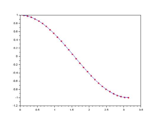
Fig. 1: Plot of the numerical solution and the exact solution.

Example 4.2

([6], p. 240, Example 2)

$$y(x)=e^{x}-\frac{1}{3}xe^{3x}+\frac{1}{3}x+\int_{0}^{x}xy^{3}(t)\mathrm{d}t$$ (17)

with the solution $y(x)=e^{x}.$

The corresponding results are given in the next Table and Fig. 2.

Successive Approximation Method		Iterative Variational Method
Iteration	Error	Iteration	Error
1	1.314327	1	4.085689
2	0.990523	2	1.844170
3	1.791381	3	1.202564
4	1.733644	4	1.073406
5	0.732878	5	1.111831
6	0.464864	6	0.700407
7	0.424189	7	0.13054
8	0.409519	8	0.004592
9	0.398283	9	0.00009
10	0.381286	10	0.000002
11	0.352116
12	0.307541
⋮	⋮
25	0.000011
26	0.000003

The used parameters to obtained the results were: $x_{f}=1.0,\ n=101,\ \varepsilon=10^{-5}.$

The maximum of absolute errors between the obtained numerical solution and the exact solution was 0.056763.

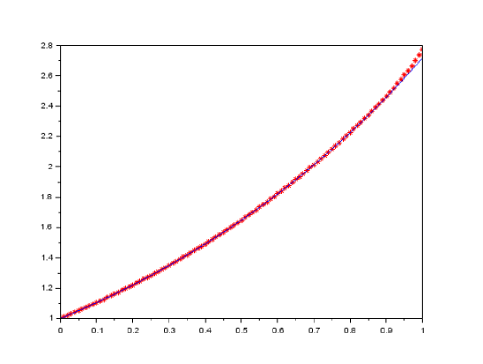
Fig. 2: Plot of the numerical solution and the exact solution.

5 Conclusions

1. The VIM as it is presented in [6], [3], when $\Lambda(x)=-1,$ for any $x,$ returns to the successive approximation method.

2. Comparing SAM with VIM we have found experimentally that VIM needs a smaller number of iterations to fulfill a stopping condition, e.g. the absolute error between two successive approximations is less than a given tolerance.

References

• [1] Inokuti M., Sekine H., Mura T., 1980, General Use of the Lagrange Multiplier in Nonlinear Mathematical Physics. In Variational Methods in Mechanics and Solids, ed. Nemat-Nasser S., Pergamon Press, 156-162.
• [2] He J.H., 2007, Variational iteration method - Some recent results and new interpretations. J. Comput. Appl. Math., 207, 3-17.
• [3] Porshokouhi M.G., Ghambari B., Rashidi M., 2011, Variational Iteration Method for Solving Volterra and Fredholm Integral Equations of Second Kind. Gen.Math. Notes, 2, no, 1, 143-148.
• [4] Bani issa M.Sh., Hamoud A.A., Giniswamy, Ghadle K.P., 2019, Solving nonlinear Volterra integral equations by using numerical technoques. Int. J. Adv. Appl. Math. and Mech., 6(4), 50-54.
• [5] Shakeri S., Saadati R., Vaezpour S.M., Vahidi J., 2009, Variational Iteration Method for Solving Integral Equations. J. of Applied Sciences, 9 (4), 799-800.
• [6] Wazwaz A-M., 2015, A First Course in Integral Equations. World Scientific, New Jersey.
• [7] Xu L., 2007, Variational iteration method for solving integral equations. Computers & mathematics with applications. 54, 1071-1078.