Revisiting model relations between T-odd transverse-momentum dependent parton distributions and generalized parton distributions

Abstract

We revisit the connection between generalized parton distributions in impact parameter space and T-odd effects in single spin asymmetries of the semi-inclusive deep inelastic process. We show that nontrivial relations can be established only under very specific conditions, typically realized only in models that describe hadrons as two-body bound systems and involving a helicity-conserving coupling between the gauge boson and the spectator system. Examples of these models are the the scalar-diquark spectator model or the quark-target model for the nucleon, and relativistic models for the pion at the lowest order in the Fock-space expansion.

Introduction

Generalized parton distributions (GPDs) and transverse momentum dependent parton distributions (TMDs) are fundamental nonperturbative objects that help unraveling the quark-gluon dynamics inside hadrons. At leading twist, there are eight independent GPDs and eight independent TMDs, in a one to one correspondence depending on the active parton and target polarizations. This correspondence arises from the projection of the fully unintegrated and off-diagonal correlator, defining the generalized transverse momentum dependent parton distributions, into two independent subspaces of the whole space spanned by the parton and target momentum Meissner et al. (2008, 2009); Lorcé and Pasquini (2013); Lorcé et al. (2011); Burkardt and Pasquini (2016). Furthermore, one can define impact-parameter dependent densities (IPDs) as the Fourier transforms of the GPDs in impact parameter space at zero longitudinal momentum transfer. The correlator of IPDs has formally the same structure as the correlator for TMDs, with the impact parameter $\bm{{b}}_{\perp}$ taking the role of the transverse momentum $\bm{{k}}_{\perp}$ Diehl and Hagler (2005); Meissner et al. (2007). Beyond this formal connection, in general it is not possible to establish model-independent relations between GPDs and TMDs. Only model calculations show nontrivial relations Meissner et al. (2007); Avakian et al. (2010); Lorcé and Pasquini (2013). The most prominent cases are the relations which describe T-odd effects in single spin asymmetries (SSAs) via factorization of the effects of final state interactions (FSIs), incorporated in a so-called “chromodynamics lensing function,” and a spatial distortion of GPDs in impact parameter space Burkardt (2002, 2004a). These relations have been established for the Sivers effect and the IPD for unpolarized partons in a transversely polarized nucleon target, using spectator models Burkardt and Hwang (2004); Bacchetta et al. (2008) and a quark target model Meissner et al. (2007), and used also in a phenomenological extraction of the Sivers function Bacchetta and Radici (2011). Furthermore, they have been discussed for the Boer-Mulders effect and a certain combination of chiral-odd IPDs describing transversely polarized quark in an unpolarized target, such as the nucleon Burkardt (2005) or the pion Burkardt and Hannafious (2008); Gamberg and Schlegel (2010); Meissner et al. (2008). However, they have been found to be violated within three-quark model calculations for the nucleon Pasquini and Yuan (2010); Pasquini et al. (2008); Boffi et al. (2003); Pasquini et al. (2005); Pasquini and Boffi (2007). More in general, it has been argued that even in the context of spectator models these relations are far from being obvious if one considers Fock-state contributions beyond the leading terms Meissner et al. (2007).

In this work, we demonstrate that very specific conditions have to be imposed on the final-state interaction in order to express T-odd TMDs in terms of an impact-parameter distortion and a lensing function. These conditions are typically fulfilled only in models where the target is described as two-body bound system and the FSI does not change any of the spectator’s quantum numbers and modifies only its transverse momentum.

The work is organized as follows. In Sec. I, we introduce the definition of the GPDs, both in momentum and impact parameter space, and of the TMDs. We then discuss the possible lensing relations between the average transverse momentum related to T-odd effects and IPDs, and the very restrictive conditions that should be imposed on the FSI for the validity of these relations. In Sec. II, we derive the lensing relation for the pion target, described in terms of the lowest $q\bar{q}$ Fock-state component. Besides the two-body nature of the system, a key ingredient for the validity of the relation is the assumption of a perturbative coupling between the spectator parton and the Wilson gluon, which gives the effects of the FSIs in a semi-inclusive deep inelastic scattering (SIDIS) process. The relation can be generalized by assuming an effective interaction vertex, which is helicity conserving and may depend only on the transverse-momentum of the exchanged gluon. In Sec. III, we consider the case of a proton target and we show that the lensing relations can not be established in a model-independent way even in the most simple case of a proton target described by the lowest-order Fock component of three quarks. Sec. IV deals with models that describe the nucleon as a two-body system, such as the models with a quark and a diquark spectator, and elucidates under which conditions one can restore the lensing relations within these models. Our conclusions are drawn in Sec. V. In the Appendix we show the derivation of the conditions that should be satisfied for the lensing relation.

I Relations between GPDs and T-odd TMDs

In this section, we summarize the arguments that lead to infer a possible nontrivial relation between T-odd TMDs and IPDs. The quark TMDs are defined through the following correlation function

$$\Phi^{[\Gamma]}\left(x,\bm{{k}_{\perp}},S\right) =\frac{1}{2}\int\frac{dz^{-}d\bm{{z}_{\perp}}}{(2\pi)^{3}}e^{ik\cdot z}\braket{p,S}{\overline{\psi}\left(-\frac{z}{2}\right)\Gamma\mathcal{W}\left(-\frac{z}{2},\frac{z}{2}\right)\psi\left(\frac{z}{2}\right)}{p,S}\Big{|}_{z^{+}=0},$$ (1)

where $p=(p^{+},p^{-},\bm{{p}}_{\perp}=\bm{{0}_{\perp}})$ and $S$ are, respectively, the hadron-target momentum and spin, $\psi$ is the quark field operator and $\Gamma$ is a generic matrix in the Dirac space. The TMDs depend on the light-cone momentum fraction

$$x=\frac{k^{+}}{P^{+}},$$ (2)

and on the quark transverse momentum $\bm{{k}_{\perp}}$.

The Wilson line $\mathcal{W}$ connecting the two quark fields ensures color gauge invariance and is defined as Collins (2002); Collins and Soper (1982); Ji and Yuan (2002); Belitsky et al. (2003); Boer et al. (2003)

$$\mathcal{W}(a,b)=\mathcal{P}\text{exp}\left\{-ig_{s}\int_{\gamma}d\zeta\cdot A(\zeta)\right\},$$

where $g_{s}$ is related to the strong coupling constant, $\alpha_{s}=g^{2}_{s}/(4\pi)$, and $\gamma$ is a path from $a$ to $b$ that is determined by the physical process under consideration (in this work, we consider the Wilson line of a SIDIS process) Collins (2002). The Wilson line in Eq. (1) breaks the naive time-reversal invariance of the correlator and, as a consequence, T-odd TMDs need to be included. At leading-twist and for spin $1/2$ targets, one has two T-odd TMDs, i.e. the Sivers function $f_{1T}^{\perp}(x,\bm{{k}}^{2}_{\perp})$ Sivers (1990, 1991) and the Boer-Mulders TMD $h_{1}^{\perp}(x,\bm{{k}}^{2}_{\perp})$ Boer and Mulders (1998). The Sivers function describes the momentum distribution of unpolarized quark in a transversely polarized target, and is obtained from the correlator (1) with $\Gamma=\gamma^{+}$. On the other hand, the Boer-Mulders function gives the momentum distribution of transversely polarized quarks in an unpolarized target, and is is defined from the correlator (1) with $\Gamma=i\sigma^{j+}\gamma_{5}$. In the case of spin-0 target, only the contribution of the Boer-Mulders functions can exist. The full list of leading-twist TMDs is shown in a schematic way in Tab. 1.

The IPDs are distribution functions in the mixed momentum and coordinate space $(x,\bm{{b}}_{\perp})$, with $\bm{{b}}_{\perp}$ being the transverse distance of the quark from the transverse center of momentum of the target Burkardt (2000). They are defined from the following quark-quark correlator

$$\mathcal{F}^{[\Gamma]}(x,\bm{{b}}_{\perp},S)=\frac{1}{2}\int\frac{dz^{-}}{2\pi}e^{ixp^{+}z^{-}}\braket{p^{+},\bm{{R}}_{\perp}=\bm{{0}}_{\perp},S}{\overline{\psi}(z_{1})\Gamma\mathcal{W}\left(z_{1},z_{2}\right)\psi\left(z_{2}\right)}{p^{+},\bm{{R}}_{\perp}=\bm{{0}}_{\perp},S},$$ (3)

where the quark fields are evaluated at $z_{1,2}=(0^{+},\mp\frac{z^{-}}{2},\bm{{b}}_{\perp})$ and the hadron is in a state with longitudinal momentum $p^{+}$ at a transverse position $\bm{{R}}_{\perp}=\bm{{0}}_{\perp}$ Burkardt (2000, 2003); Soper (1977).

The GPDs in the momentum space are defined through the following light-cone correlation function

$$F^{[\Gamma]}(x,\xi,t,S)=\frac{1}{2}\int\frac{dz^{-}}{2\pi}e^{ik\cdot z}\braket{p^{\prime},S}{\overline{\psi}\left(-\frac{z}{2}\right)\Gamma\mathcal{W}\left(-\frac{z}{2},\frac{z}{2}\right)\psi\left(\frac{z}{2}\right)}{p,S}\Big{|}_{z^{+}=0,\ \bm{{z}}_{\perp}=\bm{{0}}_{\perp}}$$ (4)

and depend, beside $x$, on the following variables

$$\xi =-\frac{\Delta^{+}}{2P^{+}}, t =\Delta^{2},$$ (5)

where $P=(p+p^{\prime})/2$ and $\Delta=p^{\prime}-p$. For $\xi=0$, the GPD correlator (4) is related to the IPD correlator (3) by a Fourier transform from the coordinates $\bm{{\Delta}}_{\perp}$ to $\bm{{b}}_{\perp}$, and, accordingly, we can obtain the IPD ${\cal X}$ from the following Fourier transform of the GPD

$${\cal X}(x,\bm{{b}}^{2}_{\perp})=\int\frac{d\bm{{\Delta}_{\perp}}}{(2\pi)^{2}}e^{-i\bm{{\Delta}}_{\perp}\cdot\bm{{b}}_{\perp}}X(x,\xi=0,-\bm{{\Delta}}^{2}_{\perp}).$$ (6)

The full list of leading-twist IPDs is shown in a schematic way in Tab. 1. At leading-twist and for spin $1/2$ targets, the correlator (3) with $\Gamma=\gamma^{+}$ and transversely polarized targets can be parametrized in terms of the derivative of the IPD $\mathcal{E}$, while with $\Gamma=i\sigma^{j+}\gamma_{5}$ and unpolarized target we access the derivative of the combination $\mathcal{E}_{T}+2\widetilde{\mathcal{H}}_{T}$ of chiral-odd IPDs. In the case of spin-zero targets, the contributions from the IPDs $\mathcal{E}$ and $\mathcal{E}_{T}$ are absent.

		quark pol.
		U	L	T
nucleon pol.	U	${\color[rgb]{0,0,0}f_{1}}$		$h_{1}^{\perp}$
	L		${\color[rgb]{0,0,0}g_{1}}$	$h_{1L}^{\perp}$
	T	$f_{1T}^{\perp}$	$g_{1T}$	$h_{1}$, $h_{1T}^{\perp}$
	Twist-2 TMDs

		quark pol.
		U	L	T
nucleon pol.	U	${\color[rgb]{0,0,0}\mathcal{H}}$		$\mathcal{E}_{T}+2\widetilde{\mathcal{H}}_{T}$
	L		${\color[rgb]{0,0,0}\widetilde{\mathcal{H}}}$
	T	$\mathcal{E}$		$\mathcal{H}_{T}$,$\widetilde{\mathcal{H}}_{T}$
	Twist-2 IPDs

Table 1: Tables of the leading-twist transverse momentum distributions (TMDs) and impact parameter distributions (IPDs) with their relation to nucleon and quark polarization states. For the complete definition, we refer to Refs. Diehl and Hagler (2005); Meissner et al. (2007).

The analogy between the tensor structure of the parametrizations of the quark TMD and IPD correlators suggests the following correspondences for the distributions of spin $1/2$ targets Diehl and Hagler (2005); Meissner et al. (2007)

$$f_{1T}^{\perp}\left(x,\bm{{k}}^{2}_{\perp}\right)\leftrightarrow-\left(\mathcal{E}\left(x,\bm{{b}}^{2}_{\perp}\right)\right)^{\prime},\quad h_{1}^{\perp}\left(x,\bm{{k}}^{2}_{\perp}\right)\leftrightarrow-\left(\mathcal{E}_{T}\left(x,\bm{{b}}^{2}_{\perp}\right)+2\widetilde{\mathcal{H}}_{T}\left(x,\bm{{b}}^{2}_{\perp}\right)\right)^{\prime},$$ (7)

where we used the following notation for the derivative of the IPDs

$$\left({\cal X}\left(x,\bm{{b}}^{2}_{\perp}\right)\right)^{\prime}=\frac{\partial}{\partial\bm{{b}}^{2}_{\perp}}{\cal X}\left(x,\bm{{b}}^{2}_{\perp}\right).$$ (8)

Similarly, the correspondence for spin-zero targets reads

$$\quad h_{1}^{\perp}\left(x,\bm{{k}}^{2}_{\perp}\right)\leftrightarrow-\left(\widetilde{\mathcal{H}}_{T}\left(x,\bm{{b}}^{2}_{\perp}\right)\right)^{\prime}.$$ (9)

In order to specify the precise form of the link in Eqs. (7), we consider the average quark transverse momentum of an unpolarized quark in a transversely polarized target given by

$$\braket{k_{\perp}^{i}(x)}_{UT}=\int d\bm{{k}}_{\perp}k^{i}_{\perp}\Phi^{[\gamma^{+}]}(x,\bm{{k}}_{\perp},\bm{{S}}_{\perp}).$$ (10)

Following the derivation in Ref. Meissner et al. (2007), Eq. (10) can be rewritten as

$$\begin{split}\braket{k_{\perp}^{i}(x)}_{UT}&=\frac{1}{2}\int\frac{dz^{-}}{2\pi}e^{ixp^{+}z^{-}}\braket{p,\bm{{S}}_{\perp}}{\overline{\psi}\left(-\frac{z}{2}\right)\mathcal{W}\left(-\frac{z}{2},\frac{z}{2}\right)\mathcal{I}^{i}\left(\frac{z}{2}\right)\gamma^{+}\psi\left(\frac{z}{2}\right)}{p,\bm{{S}}_{\perp}}\big{|}_{z^{+}=\bm{{z}_{\perp}}=0}\\ &=\frac{1}{2}\int d\bm{{b}}_{\perp}\int\frac{dz^{-}}{2\pi}e^{ixp^{+}z^{-}}\braket{p^{+},\bm{{R}}_{\perp}=\bm{{0}}_{\perp},\bm{{S}}_{\perp}}{\bar{\psi}(z_{1})\mathcal{W}(z_{1};z_{2})\mathcal{I}^{i}(z_{2})\gamma^{+}\psi(z_{2})}{p^{+},\bm{{R}}_{\perp}=\bm{{0}}_{\perp},\bm{{S}}_{\perp}}\end{split}$$ (11)

The operator $\mathcal{I}^{i}(z)$ encodes the contribution of the FSIs, and is defined as

$$\begin{split}\mathcal{I}^{i}\left(z\right)&=\frac{g_{s}}{2}\int dy^{-}\mathcal{W}\left((z^{-},z^{+},\bm{{z}_{\perp}}),(y^{-},z^{+},\bm{{z}_{\perp}})\right)G^{+i}\left(y^{-},z^{+},\bm{{z}_{\perp}}\right)\mathcal{W}\left((y^{-},z^{+},\bm{{z}_{\perp}}),(z^{-},z^{+},\bm{{z}_{\perp}})\right),\end{split}$$ (12)

with $G^{+i}$ being the gluon-field strength tensor.

As observed for the first time in Ref. Boer et al. (2003), there is a connection between the transverse-momentum weighted quark correlator in Eq. (11) and the collinear twist-3 quark-gluon-quark correlator defined as

$$i\Phi_{G}^{i}(x,x) =\int\frac{dz^{-}dy^{-}}{(2\pi)^{2}}\,e^{ixp^{+}z^{-}}\,\langle p,\bm{{S}_{\perp}}|\overline{\psi}\left(-\frac{z}{2}\right)\,\mathcal{W}\left(-\frac{z}{2},y\right)\,ig\,G^{+i}(y)\,\mathcal{W}\left(y,\frac{z}{2}\right)\,\psi\left(\frac{z}{2}\right)|p,\bm{{S}_{\perp}}\rangle\Big{|}_{\begin{subarray}{c}z^{+}=\bm{{z}_{\perp}}=0\\ y^{+}=\bm{{y}_{\perp}}=0\end{subarray}}$$ (13)

$$=\frac{M}{2}\biggl{[}-i\epsilon_{\perp}^{ij}S_{\perp}^{j}F_{FT}(x,x)\gamma^{-}+H_{FU}(x,x)\,\gamma^{i}\gamma^{-}\biggr{]}\ .$$ (14)

The decomposition contains the so-called Qiu-Sterman matrix element $F_{FT}$ Qiu and Sterman (1991) and an analogous, chiral-odd term.

Eq. (12) has a more intuitive interpretation in the light-cone gauge, $A^{+}=0$ Burkardt (2004b). In this case, the Wilson lines in the definition of $\mathcal{I}^{i}(z)$ run along the light-cone, and reduce to unity. As a result, one has

$$\mathcal{I}^{i}\left(z\right)=\frac{g_{s}}{2}\Bigl{(}A_{\perp}^{i}\left(\infty^{-},z^{+},\bm{{z}_{\perp}}\right)-A_{\perp}^{i}\left(-\infty^{-},z^{+},\bm{{z}_{\perp}}\right)\Bigr{)}.$$

The gauge, however, is not completely fixed by the condition $A^{+}=0$. The fixing of residual gauge degrees of freedom can be obtained using additional boundary conditions on the gauge potential. There are three common choices:

$$\bm{{A}_{\perp}}(\infty^{-}) =0, \bm{{A}_{\perp}}(-\infty^{-}) =0, \bm{{A}_{\perp}}(\infty^{-})+\bm{{A}_{\perp}}(-\infty^{-}) =0,$$

known, respectively, as retarded, advanced and principal value prescription. We work with the advanced boundary condition $\bm{{A}_{\perp}}(-\infty^{-})=0$, but analogous results hold for the other two prescriptions (as it should be, since all the results must be gauge invariant). Our choice leads to the following results

$$\braket{k_{\perp}^{i}(x)}_{UT} =\frac{g_{s}}{2}\int\frac{dz^{-}}{2\pi}e^{ixp^{+}z^{-}}\braket{p,\bm{{S}}_{\perp}}{\overline{\psi}\left(-\frac{z}{2}\right)A_{\perp}^{i}\left(\infty^{-}\right)\gamma^{+}\psi\left(\frac{z}{2}\right)}{p,\bm{{S}}_{\perp}}\big{|}_{z^{+}=\bm{{z}_{\perp}}=0},$$ (15)

$$\braket{k_{\perp}^{i}(x)}_{TU}^{j} =\frac{g_{s}}{2}\int\frac{dz^{-}}{2\pi}e^{ixp^{+}z^{-}}\braket{p}{\overline{\psi}\left(-\frac{z}{2}\right)A_{\perp}^{i}\left(\infty^{-}\right)i\sigma^{j+}\gamma_{5}\psi\left(\frac{z}{2}\right)}{p}\big{|}_{z^{+}=\bm{{z}_{\perp}}=0}.$$ (16)

One notices from Eq. (16) that the FSIs in the light-cone gauge with advanced boundary conditions (and, similarly, with the retarded or principal value prescriptions) reduce to the exchange of a transverse gluon at light-cone infinity between the active quark and the spectator partons.

Up to this point, the analysis is still general. In order to obtain an expression containing an IPD, some very specific conditions have to be imposed on the operator $\mathcal{I}^{i}(z)$, Using the completeness relation, we can rewrite the first line of Eq. (11) as

$$\braket{k_{\perp}^{i}(x)}_{UT} =\frac{1}{2}\int d\bm{{b}}_{\perp}\int\frac{dz^{-}}{2\pi}e^{ixp^{+}z^{-}}\operatorname*{\mathchoice{\ooalign{$\displaystyle\sum$\cr$\displaystyle\int$\cr}}{\ooalign{\raisebox{0.14pt}{\scalebox{0.7}{$\textstyle\sum$}}\cr$\textstyle\int$\cr}}{\ooalign{\raisebox{0.2pt}{\scalebox{0.6}{$\scriptstyle\sum$}}\cr$\scriptstyle\int$\cr}}{\ooalign{\raisebox{0.2pt}{\scalebox{0.6}{$\scriptstyle\sum$}}\cr$\scriptstyle\int$\cr}}}_{X,X^{\prime}}\braket{X}{\mathcal{I}^{i}(z_{2})}{X^{\prime}}$$ (25)

$$\quad\times\braket{p^{+},\bm{{R}}_{\perp}=\bm{{0}}_{\perp},\bm{{S}}_{\perp}}{\bar{\psi}(z_{1})\mathcal{W}(z_{1},z_{2})}{X}\gamma^{+}\braket{X^{\prime}}{\psi(z_{2})}{p^{+},\bm{{R}}_{\perp}=\bm{{0}}_{\perp},\bm{{S}}_{\perp}}.$$ (26)

If we introduce the Fourier transform of the quark fields $\psi(z/2)$ and $\phi\left(\frac{z}{2}\right)=\bar{\psi}\left(-\frac{z}{2}\right)\mathcal{W}\left(-\frac{z}{2};\frac{z}{2}\right)$, and use the light-front Fock expansion for the intermediate states, Eq. (26) reads as

$$\braket{k_{\perp}^{i}(x)}_{UT} =\frac{1}{2}\int\{dk_{1}\}\{dk_{2}\}\{dl\}\int\frac{dz^{-}}{2\pi}e^{ixp^{+}z^{-}}e^{-i\frac{z^{-}}{2}(k^{+}_{1}+k^{+}_{2}+l^{+})}\sum_{n,m}\sum_{\beta,\beta^{\prime}}\int\prod_{i=1}^{n}\frac{dq^{+}_{i}d\bm{q}_{\perp,i}}{(2\pi)^{3}2q_{i}^{+}}\prod_{i=1}^{m}\frac{dw^{+}_{i}d\bm{w}_{\perp,i}}{(2\pi)^{3}2w_{i}^{+}}$$

$$\times\braket{p^{+},\bm{{p}}_{\perp}=\bm{{0}_{\perp}},\bm{{S}}_{\perp}}{\phi(k_{1})\gamma^{+}}{\{q^{+}_{i},\bm{q}_{\perp,i}\}_{n}}\braket{\{q^{+}_{i},\bm{q}_{\perp,i}\}_{n},\beta^{\prime}}{I^{i}(l)}{\{w^{+}_{i},\bm{w}_{\perp,i}\}_{m}}$$

$$\times\braket{\{w^{+}_{i},\bm{w}_{\perp,i}\}_{m},\beta^{\prime}}{\psi(k_{2})}{p^{+},\bm{{p}}_{\perp}=\bm{{0}_{\perp}},\bm{{S}}_{\perp}},$$ (27)

where $\{dk\}$ is the Lorentz invariant integration measure. In Eq. (27), the index $\beta$ and $\beta^{\prime}$ label the parton, color and the helicity content of the intermediate states. As derived explicitly in the Appendix, one can obtain the factorization of the lensing function and the IPD in Eq. (27) by requiring that the matrix elements of the operator $I^{i}(l)$ satisfy the following relation

$$\braket{\{q^{+}_{i},\bm{q}_{\perp,i}\}_{n}}{I^{i}(l)}{\{w^{+}_{i},\bm{w}_{\perp,i}\}_{m}}=2\pi L^{i}\biggl{(}\frac{\bm{{l}_{\perp}}}{1-x}\biggr{)}\delta_{n,m}\delta_{\beta\beta^{\prime}}\delta(l^{+})\prod_{i=1}^{n}(2\pi)^{3}2q_{i}^{+}\delta(q^{+}_{i}-w^{+}_{i})\delta\left(\bm{q}_{\perp,i}-\bm{w}_{\perp,i}-x_{i}\frac{\bm{{l}_{\perp}}}{1-x}\right),$$ (28)

where $x_{i}$ is the light-cone momentum fraction of each constituent w.r.t. the hadron target light-cone momentum, i.e. $x_{i}=w^{+}_{i}/p^{+}$, and should satisfy the relation $\sum_{i}x_{i}=1-x$. The matrix elements of the operator $I^{i}(l)$ in Eq. (28) represent the interaction between the active parton and the spectator system mediated by the Wilson gluons and correspond to the FSIs that occur in a SIDIS process. The relation (28) imposes strict conditions that are equivalent to requiring that:

• the FSIs should connect Fock states with the same number of constituents and the same parton, helicity and color content;

• the FSIs should transfer the total transverse momentum $\bm{{l}_{\perp}}/(1-x)$ to the whole spectator system;

• the FSIs can not transfer momentum in the light-cone direction to the spectator system;

• the FSIs should transfer a fraction $x_{i}=w^{+}_{i}/p^{+}$ of the total transverse momentum to each constituent of the spectator system.

The last condition is the most stringent. It is crucial to obtain the correct transverse light-front boost that gives the nondiagonal matrix element defining the GPD and then the transverse distortion in impact parameter space described by the IPD. For convenience, we can discuss the implications of the condition $4)$ in the light-cone gauge with advanced boundary conditions, where the FSI reduces to the exchange of a transverse gluon at light-cone infinity between the active parton and the spectator system. In this case, one can easily deduce that the condition $4)$ can be realized with a perturbative coupling between the gauge boson and the active parton only if the spectator system is composed by a single constituent, i.e. the hadron target is a two-body bound system. Then, the light-cone momentum fraction of the spectator is equal to $1-x$ and the constraint on the transverse momentum transferred by the Wilson gluon to the spectator system follows trivially from the conservation of the total momentum of the hadron target. Otherwise, the condition $4)$ imposes to share the transverse momentum carried by the Wilson gluon with each spectator parton in a proportion equal to the longitudinal momentum fraction $x_{i}$. This can not be realized in systems composed by more than two constituents by assuming an interaction vertex between the gauge boson and a single constituent.

We conclude that if and only if the above conditions are fulfilled we can write

$$\begin{split}\braket{k_{\perp}^{i}(x)}_{UT}&=-\int d\bm{{k}}_{\perp}k^{i}_{\perp}\frac{\epsilon_{\perp}^{jk}k^{j}_{\perp}S^{k}_{\perp}}{M}f^{\perp}_{1T}(x,\bm{{k}}^{2}_{\perp})\\ &\approx\int d\bm{{b}}_{\perp}\mathcal{L}^{i}\bigl{(}\bm{{b}}_{\perp}/(1-x)\bigr{)}\mathcal{F}^{[\gamma^{+}]}(x,\bm{{b}}_{\perp},\bm{{S}}_{\perp})\\ &=\int d\bm{{b}}_{\perp}\mathcal{L}^{i}\bigl{(}\bm{{b}}_{\perp}/(1-x)\bigr{)}\frac{\epsilon^{jk}_{\perp}b^{j}_{\perp}S^{k}_{\perp}}{M}\left(\mathcal{E}(x,\bm{{b}}^{2}_{\perp})\right)^{\prime}.\end{split}$$ (29)

In the next sections, we will consider explicitly a few model calculations and we will discuss to which extent the conditions 1) – 4) can be satisfied.

In an analogous way, we can analyze the average quark transverse momentum of a transversely polarized quark in an unpolarized target given by

$$\braket{k_{\perp}^{i}(x)}^{j}_{TU}=\int d\bm{{k}}_{\perp}k^{i}_{\perp}\Phi^{[i\sigma^{j+}\gamma_{5}]}(x,\bm{{k}}_{\perp},S).$$ (30)

With similar steps as before, under the conditions of applicability of the lensing hypothesis, we obtain

$$\begin{split}\braket{k_{\perp}^{i}(x)}^{j}_{TU}&=-\int d\bm{{k}}_{\perp}k^{i}_{\perp}\frac{\epsilon_{\perp}^{kj}k^{k}_{\perp}}{M}h^{\perp}_{1}(x,\bm{{k}}^{2}_{\perp})\\ &\approx\int d\bm{{b}}_{\perp}\mathcal{L}^{i}\bigl{(}\bm{{b}}_{\perp}/(1-x)\bigr{)}\mathcal{F}^{[i\sigma^{j+}\gamma_{5}]}(x,\bm{{b}}_{\perp})\\ &=\int d\bm{{b}}_{\perp}\mathcal{L}^{i}\bigl{(}\bm{{b}}_{\perp}/(1-x)\bigr{)}\frac{\epsilon^{kj}_{\perp}b^{k}_{\perp}}{M}\Bigl{(}\mathcal{E}_{T}(x,\bm{{b}}^{2}_{\perp})+2\widetilde{\mathcal{H}}_{T}(x,\bm{{b}}^{2}_{\perp})\Bigr{)}^{\prime}.\end{split}$$ (31)

Alternatively, by contracting Eqs. (29) and (31) with $-\epsilon_{\perp}^{il}S^{l}_{\perp}/(2M)$ and $-\epsilon_{\perp}^{ij}/(2M)$, respectively, we can write

$$f_{1T}^{\perp(1)}(x) =\pi F_{FT}(x,x)\approx\frac{1}{4}\int d\bm{{b}}_{\perp}b_{\perp}^{i}\mathcal{L}^{i}\bigl{(}\bm{{b}}_{\perp}/(1-x)\bigr{)}\mathcal{E}^{(1)}(x,\bm{{b}}^{2}_{\perp}),$$ (32)

$$h_{1}^{\perp(1)}(x) =\pi H_{FU}(x,x)\approx\frac{1}{4}\int d\bm{{b}}_{\perp}b_{\perp}^{i}\mathcal{L}^{i}\bigl{(}\bm{{b}}_{\perp}/(1-x)\bigr{)}\left(\mathcal{E}_{T}^{(1)}(x,\bm{{b}}^{2}_{\perp})+2\widetilde{\mathcal{H}}_{T}^{(1)}(x,\bm{{b}}^{2}_{\perp})\right),$$ (33)

where we used the following notations

$$f^{(1)}(x,\bm{{k}}_{\perp}^{2}) =\frac{\bm{{k}}^{2}_{\perp}}{2M^{2}}f(x,\bm{{k}}_{\perp}^{2}),$$ (34)

$${\cal X}^{(1)}(x,\bm{{b}}^{2}_{\perp}) =-\frac{2}{M^{2}}\frac{\partial}{\partial\bm{{b}}^{2}_{\perp}}{\cal X}(x,\bm{{b}}^{2}_{\perp})=\int\frac{d\bm{{\Delta}_{\perp}}}{(2\pi)^{2}}e^{-i\bm{{\Delta}}_{\perp}\cdot\bm{{b}}_{\perp}}\frac{\bm{{\Delta}}^{2}_{\perp}}{2M^{2}}X(x,\xi=0,-\bm{{\Delta}}^{2}_{\perp}).$$ (35)

For spin-zero targets, only Eqs. (31) and (33) with $\mathcal{E}_{T}(x,\bm{{b}}^{2}_{\perp})=0$ and $2\widetilde{\mathcal{H}}_{T}\rightarrow\widetilde{\mathcal{H}}_{T}.$ survives.

II Lensing relation for the pion

In this section, we show how the relation between the Boer-Mulders function and the the chiral-odd GPD $\widetilde{\mathcal{H}}_{T}$ is realized for a spin-zero target like the pion, described as a quark-antiquark ($q\bar{q}$) bound state. In the framework of light-front quantization and working in the gauge $A^{+}=0$, the leading-order contribution of the Fock-state decomposition of a pion state with momentum $p$ is given by

$$\ket{\pi(p)}=\sum_{\{\lambda_{i}\}}\sum_{\{q_{i}\}}\int\left[Dx\right]_{2}\Psi_{q\bar{q}}(\beta,r)\delta_{c_{1}c_{2}}\ket{\lambda_{1},q_{1},c_{1},p_{1}}\ket{\lambda_{2},q_{2},c_{2},p_{2}}.$$ (36)

In Eq. (36), $\lambda_{i}$ are the quarks light-front helicities, $q_{i}=q,\bar{q}$ denotes the quark and anti-quark flavor, $c_{i}$ is a color index, and $p_{i}$ is the parton momentum. The function $\Psi_{q\bar{q}}$ is the light-front wave function (LFWF) of the $q\bar{q}$ state and its arguments are indicated with the collective notation $\beta=(\{\lambda_{i}\},\{q_{i}\})$ and $r=\{x_{i},\bm{{k}}_{\perp,i}\}$. The momentum coordinates $k_{i}$ of the partons are in the so-called “hadron” frame Diehl et al. (2001), corresponding to the reference frame where the pion has zero transverse momentum, i.e.

$$\bm{k}_{\perp,i} =\bm{p}_{\perp,i}-x_{i}\bm{{p}_{\perp}},\quad x_{i}=\frac{p_{i}^{+}}{p^{+}}=\frac{k_{i}^{+}}{p^{+}}.$$ (37)

We will refer to transverse parton momenta in the hadron frame as intrinsic transverse momenta. The integration measure in Eq. (36) is defined as

$$\left[Dx\right]_{N} =\frac{[dx]_{N}[d\bm{{k}_{\perp}}]_{N}}{\sqrt{\prod_{i=1}^{N}x_{i}}},$$ (38)

$$[dx]_{N} =\delta\left(1-\sum_{i=1}^{N}x_{i}\right)\prod_{i=1}^{N}dx_{i},$$ (39)

$$[d\bm{{k}_{\perp}}]_{N} =2(2\pi)^{3}\delta\left(\sum_{i=1}^{N}\bm{k}_{\perp,i}\right)\prod_{i=1}^{N}\frac{d\bm{k}_{\perp,i}}{2(2\pi)^{3}}.$$ (40)

The flavor and helicity structure of the parton composition in Eq. (36) can be made explicit as Ji et al. (2004)

$$\begin{split}&\ket{\pi(p)}=T_{\pi}\int\frac{dx_{1}dx_{2}}{\sqrt{x_{1}x_{2}}}\frac{d\bm{k}_{\perp,1}d\bm{k}_{\perp,2}}{2(2\pi)^{3}}\delta\left(1-x_{1}-x_{2}\right)\delta\left(\bm{k}_{\perp,2}+\bm{k}_{\perp,1}\right)\frac{\delta_{c_{1}c_{2}}}{\sqrt{3}}\\ &\quad\times\Bigl{\{}\psi^{(1)}(1,2)\left[q^{c_{1}\dagger}_{\uparrow}(1)\bar{q}^{c_{2}\dagger}_{\downarrow}(2)-q^{c_{1}\dagger}_{\downarrow}(1)\bar{q}^{c_{2}\dagger}_{\uparrow}(2)\ket{0}\right]+\psi^{(2)}(1,2)\left[\bm{k}_{L,1}q^{c_{1}\dagger}_{\uparrow}(1)\bar{q}^{c_{2}\dagger}_{\uparrow}(2)+\bm{k}_{R,1}q^{c_{1}\dagger}_{\downarrow}(1)\bar{q}^{c_{2}\dagger}_{\downarrow}(2)\ket{0}\right]\Bigr{\}},\end{split}$$ (41)

where $\bm{{k}}_{R(L),i}=k_{x,i}\pm ik_{y,i}$ and $q^{c_{i}\dagger}_{\lambda}$ and $\bar{q}^{c_{i}\dagger}_{\lambda}$ are the creation operators of quark and antiquark with helicity $\lambda$ and color $c_{i}$, respectively. In Eq. (41), $T_{\pi}$ is the isospin factor which projects on the different members of the isotriplet of the pion, and is defined as $T_{\pi}=\sum_{\tau_{q},\tau_{\bar{q}}}\braket{1/2\tau_{q}1/2\tau_{\bar{q}}}{1\tau_{\pi}}$ with $\tau_{q,\bar{q},\pi}$ the isospin of the quark, anti-quark and pion state, respectively. Furthermore, the the light-front wave amplitudes (LFWAs) $\psi^{(1)}$ and $\psi^{(2)}$ are functions of quark momenta with arguments $1,2$ representing $x_{1}$, $\bm{{k}}_{\perp,1}$ and $x_{2}$, $\bm{{k}}_{\perp,2}$, respectively, and correspond to quark states with orbital angular momentum (OAM) $l_{z}=0$ and $|l_{z}|=1$, respectively. They are scalar functions, and depend on the parton momenta only through scalar products $\bm{{k}}_{\perp,i}\cdot\bm{{k}}_{\perp,j}$. In the light-cone gauge with advanced boundary conditions for the transverse components of the gauge field, the LFWAs are complex functions Ji and Yuan (2002); Belitsky et al. (2003); Brodsky et al. (2010). Using the pion state (41), we can represent the pion GPDs and TMDs in terms of overlap of LFWAs in a model-independent way.

The pion chiral-odd GPD is defined as

$$F^{[i\sigma^{j+}\gamma_{5}]}_{\pi}(x,\Delta^{+},\bm{{\Delta}}_{\perp}) =-\frac{i\epsilon_{\perp}^{kj}\Delta^{k}_{\perp}}{M_{\pi}}\widetilde{H}_{T,\pi}(x,\xi,-\bm{{\Delta}}_{\perp}^{2}),$$ (42)

where $\epsilon_{\perp}^{ij}=\epsilon^{+-ij}$. Introducing the following overlap of LFWAs for the $q\bar{q}$ component of the pion

$$G^{k}\left(1,1^{\prime}\right) =F^{k}\bigl{(}x_{1},\bm{k}_{\perp,1};1-x_{1},-\bm{k}_{\perp,1}\bigr{|}\bigl{|}x^{\prime}_{1},\bm{k}^{\prime}_{\perp,1};1-x^{\prime}_{1},-\bm{k}^{\prime}_{\perp,1}\bigr{)},$$ (43)

$$F^{k}\left((1,2\right|\left|1^{\prime},2^{\prime}\right)) =k_{\perp,1}^{k}\psi^{(2)}(1,2)\psi^{(1)*}(1^{\prime},2^{\prime})-k^{\prime k}_{\perp,1}\psi^{(1)}(1,2)\psi^{(2)*}(1^{\prime},2^{\prime}),$$ (44)

one finds at $\xi=0$

$$\frac{\Delta_{\perp}^{k}}{2M_{\pi}}\widetilde{H}_{T,\pi}(x,0,-\bm{{\Delta}}_{\perp}^{2})=\frac{T_{\pi}^{2}}{2(2\pi)^{3}}\int d\bm{{k}_{\perp}}G^{k}\left(x,\bm{{k}_{\perp}}\right|\left|x,\bm{{k}_{\perp}}+(1-x)\bm{{\Delta}_{\perp}}\right).$$ (45)

Note that the Wilson line in the light-cone correlator defining the GPDs formally reduce to the identity in the light-cone gauge $A^{+}=0$. We can Fourier transform the integral in Eq. (45), with the result

$$\begin{split}\int d\bm{{k}_{\perp}}G^{k}\left(x,\bm{{k}_{\perp}}\right|\left|x,\bm{{k}_{\perp}}+(1-x)\bm{{\Delta}_{\perp}}\right)&=\int d\bm{{k}_{\perp}}\int d\bm{{A}_{\perp}}d\bm{{B}_{\perp}}e^{-i\bm{{A}_{\perp}}\cdot\bm{{k}_{\perp}}+i\bm{{B}_{\perp}}\cdot(\bm{{k}_{\perp}}+(1-x)\bm{{\Delta}_{\perp}})}\mathcal{G}^{k}\left(x,\bm{{A}_{\perp}}\right|\left|x,\bm{{B}_{\perp}}\right)\\ &=\int d\bm{{B}_{\perp}}e^{i(1-x)\bm{{B}_{\perp}}\cdot\bm{{\Delta}_{\perp}}}\mathcal{G}^{k}\left(x,\bm{{B}_{\perp}}\right|\left|x,\bm{{B}_{\perp}}\right).\end{split}$$ (46)

Using this expression, Eq. (45) can easily be transformed into the impact parameter $\bm{{b}_{\perp}}$ space to obtain the pion chiral-odd IPD

$$\begin{split}\frac{ib_{\perp}^{k}}{M_{\pi}}\left(\widetilde{\mathcal{H}}_{T,\pi}(x,\bm{{b}}_{\perp}^{2})\right)^{\prime}&=\int\frac{d\bm{{\Delta}_{\perp}}}{(2\pi)^{2}}e^{-i\bm{{b}_{\perp}}\cdot\bm{{\Delta}_{\perp}}}\left(\frac{\Delta_{\perp}^{k}}{2M_{\pi}}H_{T,\pi}(x,0,-\bm{{\Delta}}_{\perp}^{2})\right)\\ &=\frac{T_{\pi}^{2}}{2(2\pi)^{3}}\int\frac{d\bm{{\Delta}_{\perp}}}{(2\pi)^{2}}e^{-i\bm{{b}_{\perp}}\cdot\bm{{\Delta}_{\perp}}}\int d\bm{{B}_{\perp}}e^{i(1-x)\bm{{B}_{\perp}}\cdot\bm{{\Delta}_{\perp}}}\mathcal{G}^{k}\left(x,\bm{{B}_{\perp}}\right|\left|x,\bm{{B}_{\perp}}\right)\\ &=\frac{T_{\pi}^{2}}{2(2\pi)^{5}(1-x)^{2}}\mathcal{G}^{k}\left(x,\frac{\bm{{b}_{\perp}}}{1-x}\right|\left|x,\frac{\bm{{b}_{\perp}}}{1-x}\right).\end{split}$$ (47)

The same Dirac structure giving the GPD $\widetilde{H}_{T,\pi}$ in Eq. (45) enters the correlator that defines the Boer-Mulders TMD, i.e.

$$\Phi^{[i\sigma^{j+}\gamma_{5}]}_{\pi}=-\frac{\epsilon_{\perp}^{kj}k^{k}_{\perp}}{M_{\pi}}h_{1,\pi}^{\perp}(x,\bm{{k}}_{\perp}^{2}).$$ (48)

The tensor structures in Eqs. (42) and (48) have opposite behavior under time reversal, which reveals the T-even and T-odd nature of $\widetilde{H}_{T,\pi}$ and $h_{1,\pi}^{\perp}$, respectively. This crucial difference reflects on the fact that the Boer-Mulders function would be zero without the contribution of the Wilson line. In the light-cone gauge, the contribution along the light-cone direction vanishes, and there remains a residual contribution from the transverse link at $\xi^{-}=\infty^{-}$. As outlined in Sec. I, in the calculation of the average transverse momentum of the Boer-Mulders effect the Wilson line reduces to the exchange of one Wilson gluon between the active quark and the spectator system (see Eq. (16)). If we describe the pion as a bound $q\bar{q}$ system, the corresponding cut diagram can be represented as in Fig. 1, where the blob indicates an effective coupling between the antiquark and the Wilson gluon

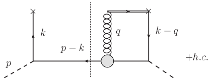
Figure 1: Cut diagram contributing to the average transverse momentum of T-odd effects in single-spin asymmetries of a SIDIS process, in the $A^{+}=0$ gauge and for a pion target in the $q\bar{q}$ configuration.

We will assume that the coupling is perturbative and consider only the tree level graph. In this framework, the LFWA overlap representation of the Boer-Mulders function has been derived in Ref. Pasquini and Schweitzer (2014) and reads

$$k_{\perp}^{k}h_{1,\pi}^{\perp}\left(x,\bm{{k}_{\perp}}^{2}\right)=\frac{2\alpha_{s}}{(2\pi)^{4}}\frac{4}{3}T_{\pi}^{2}M_{\pi}\int\frac{d\bm{{q}_{\perp}}}{\bm{{q}_{\perp}}^{2}}G^{k}\left(x,\bm{{k}_{\perp}}\right|\left|x,\bm{{k}_{\perp}}-\bm{{q}_{\perp}}\right),$$ (49)

where $\bm{{q}_{\perp}}$ is the transverse momentum of the Wilson gluon (we recall that $q^{+}=0$ in the eikonal approximation in the light cone gauge). We note that Eq. (49) involves the same overlap of LFWAs as in Eq. (45) for the case of the GPD $\widetilde{H}_{T,\pi}$. With the formal identification of

$$-\bm{{q}_{\perp}}=(1-x)\bm{{\Delta}_{\perp}},$$ (50)

the $G^{k}$ functions in Eqs. (45) and (49) have the same momentum dependence. This is crucial to recover the lensing function relation. Using Eq. (49), we can now calculate the average transverse momentum of the Boer-Mulders effect

$$\begin{split}\braket{k_{\perp}^{i}}^{j}_{TU}&=-\int d\bm{{k}_{\perp}}k_{\perp}^{i}\frac{\epsilon_{\perp}^{kj}k^{k}_{\perp}}{M_{\pi}}h_{1,\pi}^{\perp}=-\frac{2\alpha_{s}}{(2\pi)^{4}}\frac{4}{3}T_{\pi}^{2}\int\frac{d\bm{{q}_{\perp}}}{\bm{{q}_{\perp}}^{2}}\int d\bm{{k}_{\perp}}k_{\perp}^{i}\epsilon_{\perp}^{kj}G^{k}\left(x,\bm{{k}_{\perp}}\right|\left|x,\bm{{k}_{\perp}}-\bm{{q}_{\perp}}\right)\\ &=-\frac{2\alpha_{s}}{(2\pi)^{4}}\frac{4}{3}T_{\pi}^{2}\int\frac{d\bm{{q}_{\perp}}}{\bm{{q}_{\perp}}^{2}}\int d\bm{{k}_{\perp}}k_{\perp}^{i}\epsilon_{\perp}^{kj}\int d\bm{{A}_{\perp}}d\bm{{B}_{\perp}}e^{-i\bm{{A}_{\perp}}\cdot\bm{{k}_{\perp}}}e^{i\bm{{B}_{\perp}}\cdot(\bm{{k}_{\perp}}-\bm{{q}_{\perp}})}\mathcal{G}^{k}\left(x,\bm{{A}_{\perp}}\right|\left|x,\bm{{B}_{\perp}}\right)\\ &=-i\frac{4}{3}4\pi\alpha_{s}(1-x)^{3}\int d\bm{{B}_{\perp}}\int\frac{d\bm{{q}_{\perp}}}{\bm{{q}_{\perp}}^{2}}\frac{\epsilon_{\perp}^{kj}B_{\perp}^{k}}{M_{\pi}}q_{\perp}^{i}e^{-i\bm{{B}_{\perp}}\cdot\bm{{q}_{\perp}}}\left(\widetilde{\mathcal{H}}_{T,\pi}(x,\bm{{B}}_{\perp}^{2}(1-x)^{2})\right)^{\prime},\end{split}$$ (51)

where we used the following relation

$$\begin{split}\int d\bm{{k}_{\perp}}k_{\perp}^{i}&\int d\bm{{A}_{\perp}}d\bm{{B}_{\perp}}e^{-i\bm{{A}_{\perp}}\cdot\bm{{k}_{\perp}}}e^{i\bm{{B}_{\perp}}\cdot(\bm{{k}_{\perp}}-\bm{{q}_{\perp}})}\mathcal{G}^{k}\left(x,\bm{{A}_{\perp}}\right|\left|x,\bm{{B}_{\perp}}\right)=\frac{q^{i}_{\perp}}{2}\int d\bm{{B}_{\perp}}e^{-i\bm{{B}_{\perp}}\cdot\bm{{q}_{\perp}}}{\cal G}^{k}(x,\bm{{B}_{\perp}}||x,\bm{{B}_{\perp}})\\ &=iq^{i}_{\perp}(1-x)^{3}\frac{(2\pi)^{5}}{M_{\pi}T^{2}_{\pi}}\int d\bm{{B}_{\perp}}B^{k}_{\perp}\left(\widetilde{\mathcal{H}}_{T,\pi}(x,\bm{{B}_{\perp}}^{2}(1-x)^{2}))\right)^{\prime}e^{-i\bm{{B}_{\perp}}\cdot\bm{{q}_{\perp}}}.\end{split}$$

With the variable change $\bm{{B}}_{\perp}\rightarrow\bm{{b}}_{\perp}/(1-x)$ in Eq. (51), we then find

$$\braket{k_{\perp}^{i}}^{j}_{TU}=\int d\bm{{b}_{\perp}}\frac{\epsilon_{\perp}^{kj}b^{k}_{\perp}}{M_{\pi}}\mathcal{L}^{i}\left(\bm{{b}_{\perp}}/(1-x)\right)\left(\widetilde{\mathcal{H}}_{T,\pi}(x,\bm{{b}}_{\perp}^{2})\right)^{\prime},$$ (52)

where we introduced the lensing function Burkardt and Hwang (2004)

$$\mathcal{L}^{i}\left(\bm{{b}_{\perp}}/(1-x)\right)=-i\frac{4}{3}\alpha_{s}4\pi\int\frac{d\bm{q}_{\perp}}{\bm{{q}_{\perp}}^{2}}q_{\perp}^{i}e^{-i\frac{\bm{{b}_{\perp}}\cdot\bm{{\bm{q}}}_{\perp}}{(1-x)}}=-\frac{8}{3}\alpha_{s}4\pi^{2}\frac{b^{i}_{\perp}}{\bm{{b}}_{\perp}^{2}}(1-x).$$ (53)

A few comments are in order. This result relies on the assumption that the coupling between the Wilson gluon and the spectator parton is perturbative, i.e. it is described by the tree-level QCD vertex. The coupling, at leading power of $1/Q\simeq 1/p^{+}$, conserves the helicity of the spectator parton. Therefore, the helicity flip of the active quark must be compensated by a change of the OAM carried by the partons in the initial and final states. This situation is equivalent to the GPD case, where the active and spectator quarks do not change the helicity and the helicity flip of the target must be compensated by a transfer of OAM between the partons in the initial and final states.

Due to the two-body nature of the problem ($q\bar{q}$ system) the role of the transverse momentum of the gluon $\bm{{q}_{\perp}}$ is the same as the external transverse momentum $\bm{{\Delta}_{\perp}}$ in the GPD case. This can be traced back to the fact that the parton distributions should be invariant by light-front transverse boosts and depend on the intrinsic transverse-momentum coordinates of the partons. In the case of the average transverse-momentum of the Boer-Mulders effect, there is no change of the transverse momentum of the pion between the initial and final state. However, the quark and anti-quark have a different intrinsic transverse momentum in the initial and final states due to the gluon exchange. In the GPD case, the momentum transferred to the pion is absorbed by the active quark, while the transverse-momentum of the spectator quark does not change in the initial and final states. In terms of the intrinsic transverse momentum coordinates (37) in the hadron-in and hadron-out frame of the initial and final hadrons, respectively, both the active and spectator quarks experience a transfer of transverse momentum. Therefore, one can make the formal identification of Eq. (50) in the momentum dependence of the LFWAs describing the contribution of the internal parton dynamics and the effect of the FSIs can be factorized in the lensing function. In the next section, we will see that in the case of a three body system this correspondence can not be established, and, as a consequence, the lensing-function relation breaks down.

If we do not assume a perturbative coupling between the Wilson gluon and the anti-quark spectator, we may have an effective vertex that depends on the momenta of the gluon and of the anti-quark. The coupling with the Wilson gluon may occur with or without flip of the helicity of the anti-quark. In the first case, the lensing relation can not hold, as it will be discussed in Sec. IV. If the helicity flip is not allowed, the lensing relation can still be spoiled by the dependence of the vertex on the momentum of the anti-quark. By introducing an effective vertex with a general parametrization $\Lambda\left(\bm{{k}_{\perp}}^{2},\bm{{q}_{\perp}}^{2},\bm{{k}_{\perp}}\cdot\bm{{q}_{\perp}}\right)\gamma^{+}$, the average transverse momentum of the Boer-Mulders effect in Eq. (51) becomes

$$\braket{k_{\perp}^{i}}^{j}_{TU} =-\frac{2\alpha_{s}}{(2\pi)^{4}}\frac{4}{3}T_{\pi}^{2}\int d\bm{{k}_{\perp}}k_{\perp}^{i}\epsilon_{\perp}^{kj}\int\frac{d\bm{{q}_{\perp}}}{\bm{{q}_{\perp}}^{2}}G^{k}\left(x,\bm{{k}_{\perp}}\right|\left|x,\bm{{k}_{\perp}}-\bm{{q}_{\perp}}\right)\Lambda\left(\bm{{k}_{\perp}}^{2},\bm{{q}_{\perp}}^{2},\bm{{k}_{\perp}}\cdot\bm{{q}_{\perp}}\right)$$

$$=-\frac{2\alpha_{s}}{(2\pi)^{4}}\frac{4}{3}T_{\pi}^{2}\Bigg{\{}\int d\bm{{B}_{\perp}}d\bm{{A}_{\perp}}\int\frac{d\bm{{q}_{\perp}}}{\bm{{q}_{\perp}}^{2}}e^{-i\bm{{B}_{\perp}}\cdot\bm{{q}_{\perp}}}\frac{q_{\perp}^{i}}{2}\epsilon_{\perp}^{kj}\mathcal{G}^{k}\left(x,\bm{{B}_{\perp}}-\bm{{A}_{\perp}}\right|\left|x,\bm{{B}_{\perp}}\right)\widetilde{\Lambda}\left(\bm{{A}_{\perp}}^{2},\bm{{q}_{\perp}}^{2},\bm{{A}_{\perp}}\cdot\bm{{q}_{\perp}}\right)$$

$$\quad+\frac{i}{2}\int d\bm{{B}_{\perp}}d\bm{{A}_{\perp}}\ \int\frac{d\bm{{q}_{\perp}}}{\bm{{q}_{\perp}}^{2}}e^{-i\left(\bm{{B}_{\perp}}+\bm{{A}_{\perp}}\right)\cdot\frac{\bm{{q}_{\perp}}}{2}}\epsilon_{\perp}^{kj}$$

$$\quad\times\partial_{A_{\perp,i}}\left[\mathcal{G}^{k}\Big{(}x,\bm{{A}_{\perp}}\Big{|}\Big{|}x,\frac{\bm{{B}_{\perp}}+\bm{{A}_{\perp}}}{2}\Big{)}\widetilde{\Lambda}\left(\left(\frac{\bm{{B}_{\perp}}-\bm{{A}_{\perp}}}{2}\right)^{2},\bm{{q}_{\perp}}^{2},\frac{\bm{{B}_{\perp}}\cdot\bm{{q}_{\perp}}-\bm{{A}_{\perp}}\cdot\bm{{q}_{\perp}}}{2}\right)\right]\Bigg{\}}.$$ (54)

In Eq. (54), it is impossible to factorise a term like $\mathcal{G}\left(x,\bm{{B}_{\perp}}\right|\left|x,\bm{{B}_{\perp}}\right)$ and recognize the definition of the IPD, as done in Eq. (51). However, if the effective vertex depends only on $\bm{{q}_{\perp}}$, then the lensing relation (52) still holds, with the following new definition of the lensing function

$$\mathcal{L}^{i}\left(\bm{{b}_{\perp}}/(1-x)\right)=-i\frac{4}{3}\alpha_{s}4\pi\int\frac{d\bm{q}_{\perp}}{\bm{{q}_{\perp}}^{2}}q_{\perp}^{i}\Lambda(\bm{{q}_{\perp}}^{2})e^{-i\frac{\bm{{b}_{\perp}}\cdot\bm{{\bm{q}}}_{\perp}}{(1-x)}}.$$ (55)

III Lensing relation for the proton

In this section we discuss the validity of the lensing relations in Eq. (7) for the proton system. For illustration, we will consider in detail the relation between the Sivers TMD and the IPD $\mathcal{E}$. However, the same arguments can be applied for the relation involving the Boer-Mulders TMD and the combination $\mathcal{E}_{T}+2\widetilde{\mathcal{H}}_{T}$ of chiral-odd IPDs

We limit ourselves to analyzing the general structure of the LFWA overlap representation of the GPDs and the Sivers function, since the explicit dependence on the LFWAs is not relevant for our purposes. We refer to Boffi et al. (2003); Pasquini and Yuan (2010) for the full calculation. We introduce the LFWAs overlap $F_{T}\bigl{(}x_{1},\bm{k}_{\perp,1};x_{2},\bm{k}_{\perp,2};x_{3},\bm{k}_{\perp,3}\bigr{|}\bigl{|}x^{\prime}_{1},\bm{k}^{\prime}_{\perp,1};x^{\prime}_{2},\bm{k}^{\prime}_{\perp,2};x^{\prime}_{3},\bm{k}^{\prime}_{\perp,3}\big{)}$ and define the function $G_{T}$ as

$$G_{T}\left(x_{1},\bm{k}_{\perp,1};x_{2},\bm{k}_{\perp,2}\big{|}\big{|}x^{\prime}_{1},\bm{k}^{\prime}_{\perp,1};x^{\prime}_{2},\bm{k}^{\prime}_{\perp,2}\right)$$

$$\ =F_{T}\left(x_{1},\bm{k}_{\perp,1};x_{2},\bm{k}_{\perp,2};1-x_{1}-x_{2},-\bm{k}_{\perp,1}-\bm{k}_{\perp,2}\big{|}\big{|}x^{\prime}_{1},\bm{k}^{\prime}_{\perp,1};x^{\prime}_{2},\bm{k}^{\prime}_{\perp,2};1-x^{\prime}_{1}-x^{\prime}_{2},-\bm{k}^{\prime}_{\perp,1}-\bm{k}^{\prime}_{\perp,2}\right),$$

where the arguments on the right-hand side of $||$ refer to the momentum dependence of the complex conjugate LFWF of the proton in the final state, and the arguments on the left-hand side give the momentum dependence of the LFWF of the proton in the initial state.

The GPD $E$ in the limit of $\xi=0$ is obtained from the quark-quark correlator (4) with $\Gamma=\gamma^{+}$ and transversely polarized proton. The incoming and outgoing quark momenta are related by $p^{\prime}_{i}=p_{i}$ $(i\neq j)$ for the spectator quarks and $p^{\prime}_{j}=p_{j}+\Delta$ for the active quark that takes the momentum transfer to the proton. The intrinsic momenta are then obtained via the transverse-boost in Eq. (37) and are related as

$$x^{\prime}_{i} =x_{i}, \bm{{k}}^{\prime}_{\perp,i} =\bm{{k}}_{\perp,i}-x_{i}\bm{{\Delta}_{\perp}}, \text{for }i\neq j,$$ (56)

$$x^{\prime}_{j} =x_{j}, \bm{{k}}^{\prime}_{\perp,j} =\bm{{k}}_{\perp,j}+(1-x_{j})\bm{{\Delta}_{\perp}}.$$ (57)

Using momentum conservation for the intrinsic variables, i.e., $\sum_{i}x_{i}=1$ and $\sum_{i}\bm{{k}}_{\perp,i}=\bm{{0}_{\perp}}=\sum_{i}\bm{{k}}^{\prime}_{\perp,i}$, one finds the following LFWF overlap representation Boffi et al. (2003)

$$\frac{i\epsilon_{\perp}^{ij}\Delta^{j}_{\perp}S_{T}^{i}}{M}E(x,\xi=0,-\bm{{\Delta}_{\perp}}^{2})=\frac{1}{4(2\pi)^{6}}\int d\bm{{k}_{\perp}}\int_{0}^{x}dy\int d\bm{{t}_{\perp}}G_{T}\left(x,\bm{{k}_{\perp}};y,\bm{{t}_{\perp}}\right|\left|x,\bm{{k}_{\perp}}+(1-x)\bm{{\Delta}_{\perp}};y,\bm{{t}_{\perp}}-y\bm{{\Delta}_{\perp}}\right).$$ (58)

The results for the IPD distribution are then obtained taking the Fourier transform of Eq. (58) w.r.t. $\bm{{b}_{\perp}}$ and expressing $G_{T}$ in terms of its Fourier integral. One finds

$$-\frac{\epsilon_{\perp}^{ij}b_{\perp}^{j}S_{T}^{i}}{M}\left(\mathcal{E}(x,\xi=0,\bm{{b}_{\perp}}^{2})\right)^{\prime}=\frac{1}{4(2\pi)^{8}}\frac{1}{1-x}\int_{0}^{x}dy\int d\bm{{B}_{\perp}}\mathcal{G}_{T}\left(x,\frac{y\bm{{B}_{\perp}}-\bm{{b}_{\perp}}}{1-x};y,\bm{{B}_{\perp}}\right|\left|x,\frac{y\bm{{B}_{\perp}}-\bm{{b}_{\perp}}}{1-x};y,\bm{{B}_{\perp}}\right).$$ (59)

The LFWF overlap representation of the Sivers function has been derived in Ref. Pasquini and Yuan (2010), using the $3q$ component of the nucleon state and the one-gluon exchange approximation, with a perturbative quark-gluon coupling. It is given by the same function $G_{T}$ as for the GPD $E$, but with different arguments, i.e.,

$$\frac{\epsilon_{\perp}^{ij}k^{j}_{\perp}S_{T}^{i}}{M}f_{1T}^{\perp}\left(x,\bm{{k}_{\perp}}^{2}\right)=-\frac{\alpha_{s}}{3(2\pi)^{7}}\int\frac{d\bm{{q}_{\perp}}}{\bm{{q}_{\perp}}^{2}}\int_{0}^{x}dy\int d\bm{{t}_{\perp}}G_{T}\left(x,\bm{k}_{\perp};y,\bm{t}_{\perp}\right|\left|x,\bm{{k}_{\perp}}-\bm{{q}_{\perp}};y,\bm{{t}_{\perp}}+\bm{{q}_{\perp}}\right).$$ (60)

From this expression, one clearly sees that the formal identification in Eq. (50) does not apply in the case of Eqs. (58) and (60), since $(1-x)$ and $y$ are independent variables. As we will see, this is sufficient to break the lensing-function relation in the case of the proton.

From Eq. (60), one can calculate the average transverse momentum of the Sivers effect as

$$\begin{split}\braket{k_{\perp}^{i}}_{UT}&=-\int d\bm{{k}_{\perp}}k_{\perp}^{i}\frac{\epsilon_{\perp}^{ij}k^{j}_{\perp}S_{T}^{i}}{M}f_{1T}^{\perp}\\ &=\alpha_{s}\frac{M}{3(2\pi)^{7}}\int d\bm{{k}_{\perp}}k_{\perp}^{i}\int\frac{d\bm{{q}_{\perp}}}{\bm{{q}_{\perp}}^{2}}\int_{0}^{x}dy\int d\bm{{t}_{\perp}}G_{T}\left(x,\bm{k}_{\perp};y,\bm{t}_{\perp}\right|\left|x,\bm{{k}_{\perp}}-\bm{{q}_{\perp}};y,\bm{{t}_{\perp}}+\bm{{q}_{\perp}}\right)\\ &=\alpha_{s}\frac{M}{3(2\pi)^{7}}\int_{0}^{x}dy\int d\bm{{A}_{\perp}}d\bm{{B}_{\perp}}\int\frac{d\bm{{q}_{\perp}}}{\bm{{q}_{\perp}}^{2}}\frac{q_{\perp}^{i}}{2}e^{i\bm{{q}_{\perp}}\cdot\bm{{A}_{\perp}}}\mathcal{G}_{T}\left(x,\bm{{B}_{\perp}}-\bm{{A}_{\perp}};y,\bm{{B}_{\perp}}\right|\left|x,\bm{{B}_{\perp}}-\bm{{A}_{\perp}};y,\bm{{B}_{\perp}}\right)\\ &=-i\alpha_{s}\frac{M}{6(1-x)(2\pi)^{6}}\ \int_{0}^{x}dy\int d\bm{{b}_{\perp}}d\bm{{B}_{\perp}}\frac{b_{\perp}^{i}}{\bm{{b}_{\perp}}^{2}}\mathcal{G}_{T}\left(x,\frac{\bm{{B}_{\perp}}-\bm{{b}_{\perp}}}{1-x};y,\bm{{B}_{\perp}}\right|\left|x,\frac{\bm{{B}_{\perp}}-\bm{{b}_{\perp}}}{1-x};y,\bm{{B}_{\perp}}\right).\end{split}$$ (61)

Comparing this equation with Eq. (59), we immediately notice that the different dependence of the function $G_{T}$ on $\bm{{B}_{\perp}}$ does not allow us to factorize the contribution of the IPD from a lensing function. This can be traced back to the fact that in the LFWF overlap representation of the GPD the transverse momentum $\bm{{\Delta}_{\perp}}$ appears multiplied by both $(1-x)$ and $y$, since both the two spectator quarks have different intrinsic transverse momentum in the initial and final states. In other words, the transverse boost (37) from a given frame to the hadron frames transforms the transverse-momentum coordinates of the two spectator quarks in a different way, depending on their fraction $x_{i}$ of longitudinal momentum. Vice versa, in the TMD case the hadron does not change the transverse momentum in the initial and final states, and the gluon interaction occurs between the active quark and a single spectator quark, leaving unchanged the intrinsic momentum of the other spectator quark.

The failure of the lensing relation is ultimately due to the three-body structure of the nucleon LFWF, and persists more in general for any hadron system described by more than two constituent partons. Therefore the lensing relation is spoiled also for the pion when considering Fock-state components beyond the leading-order $q\bar{q}$ state. For the nucleon, one may recover the lensing relation in models where the nucleon is described as a two-body system, such as the models with a quark and a diquark spectator. However, one has to distinguish between different variants of diquark-spectator models, depending on the spin structure of the diquark and its coupling with the Wilson gluon, as we will discuss in the following section.

IV Diquark spectator models for the nucleon

The basic idea of spectator models is to evaluate the quark-quark correlators entering the definition of the TMDs and of the GPDs by inserting a complete set of intermediate states and then truncating this set at tree level to a single on-shell spectator diquark state, i.e., a state with the quantum numbers of two quarks. The diquark can be either an isospin singlet with spin 0 (scalar diquark) or an isospin triplet with spin 1 (axial-vector diquark). The target is then seen as made of an off-shell quark and an on-shell diquark. Spectator models differ by their specific choice of the target-quark-diquark vertex, of the polarization four-vectors associated with the axial-vector diquark, and of the vertex form factor that takes into account the composite nature of the target in an effective way. The approximation of a diquark spectator spoils part of the richness of the nonperturbative structure of the proton, that cannot be captured by the vertex form factor alone. Moreover, some models may introduce relations (like the lensing relation, but not only) that do not hold in general and are due to the simplifications introduced by the models themselves. A review of model-induced relations between different TMDs and between TMDs and GPDs can be found in Refs. Meissner et al. (2008); Avakian et al. (2010); Lorcé and Pasquini (2011).

The lensing relations hold in the scalar spectator models, as it was first shown in Ref. Burkardt (2004a). The arguments which lead to the lensing relations are essentially the same as discussed in Sec. II for the pion, i.e., the hadron described as a two-body system and the assumption of a perturbative helicity-conserving coupling between the gauge boson and the spectator system. For the axial-vector diquark model (AVDQ), the validity of the lensing-function relations depends on the helicity-structure of the diquark. One way to classify AVDQ models is to distinguish between models that allow for the presence of a longitudinal polarization and models that admit only transverse polarizations for the axial-vector diquark. The first class corresponds to the AVDQ models that can not satisfy the lensing relations, in contrast to the second group.

To illustrate this, we introduce the polarization vectors of the AVDQ (see, e.g., Ref. Bacchetta et al. (2008)):

$$\varepsilon_{+1}(l) =\left(0,\frac{-l_{R}}{\sqrt{2}l^{+}},{\bm{\varepsilon}}_{+1,\perp}\right),$$ (62)

$$\varepsilon_{-1}(l) =\left(0,\frac{-l_{L}}{\sqrt{2}l^{+}},\bm{\varepsilon}_{-1,\perp}\right),$$ (63)

$$\varepsilon_{0}(l) =\frac{1}{M_{a}}\left(l^{+},\frac{l_{\perp}^{2}-M_{a}^{2}}{2l^{+}},\bm{{l}_{\perp}}\right),$$ (64)

where $M_{a}$ is the AVDQ mass, $l\equiv p-k$, and:

$$\bm{\varepsilon}_{+1,\perp}=-\left(\bm{\varepsilon}_{-1,\perp}\right)^{*}=-\frac{1}{\sqrt{2}}\left(1,i\right).$$

Here we do not consider the (unphysical) time-like polarization that is discussed in Ref. Bacchetta et al. (2008). The polarization vectors in Eqs. (62)-(64) satisfy the following relations: $\varepsilon_{+1}(l)\cdot\varepsilon^{*}_{-1}(l^{\prime})=0$ for any value of $l,l^{\prime}$, whereas $\varepsilon_{\pm 1}(l)\cdot\varepsilon^{*}_{0}(l)=0$ and $\varepsilon_{\pm 1}(l)\cdot\varepsilon^{*}_{0}(l^{\prime})\neq 0$ for $l\neq l^{\prime}$. The interaction between the diquark and the gluon is given by the following coupling tensor

$$\frac{i}{e_{c}}\Gamma_{\nu\sigma}^{\rho}=(2l+q)^{\rho}g_{\nu\sigma}-(l+(1+\kappa_{a})q)_{\sigma}\delta^{\rho}_{\nu}-(l-\kappa_{a}q)_{\nu}\delta^{\rho}_{\sigma},$$ (65)

where $e_{c}$ and $\kappa_{a}$ are, respectively, the diquark color charge and the diquark anomalous chromomagnetic moment, which takes into account that the diquark is not a point-like massive axial particle, but is an effective constituent degree of freedom. In the calculation of the T-odd TMDs, the indices of the coupling tensor (65) are saturated with the gluon propagator and the AVDQ polarization vector (see Fig. 2). The contraction of the coupling tensor with the polarization vectors of the axial-vector diquark gives the following interaction vertex

$$\mathcal{R}^{\rho}=\sum_{\lambda_{1},\lambda_{2}=\pm 1,0}\varepsilon^{\nu*}_{\lambda_{1}}(l)\varepsilon^{\sigma}_{\lambda_{2}}(l+q)\Gamma_{\nu\sigma}^{\rho}.$$ (66)

This expression can be compared with the corresponding $\bar{q}g\bar{q}$ interaction vertex, which enters the calculation of the Boer-Mulders function of the pion, i.e.

$$\mathcal{R}^{\rho}=\sum_{\lambda_{1},\lambda_{2}=\pm 1/2}\bar{v}_{\lambda_{1}}(l+q)\gamma^{\rho}v_{\lambda_{2}}(l).$$ (67)

In both cases, the vertex function has the following scaling behavior

$$\mathcal{R}^{+} \simeq\mathcal{O}(p^{+}), \mathcal{R}^{i}_{\perp} \simeq\mathcal{O}(1), \mathcal{R}^{-} \simeq\mathcal{O}(1/p^{+}).$$ (68)

However, in the case of the pion, the leading-order term $\mathcal{R}^{+}$ in Eq. (67) is helicity conserving, whereas the leading contribution $\mathcal{R}^{+}$ in Eq. (66) for the axial-vector diquark contains terms that flip the helicity of the diquark. As a result, the following transitions are allowed for the AVDQ interacting with the Wilson gluon

$$\lambda_{a}=\pm 1\leftrightarrow\lambda_{a}=0,\pm 1.$$

In the calculations of the GPDs, the Wilson line in the light-cone gauge reduces to unity, and the spectator can not flip the helicity between the initial and final states. We conclude that the LFWA overlaps must be different for the average transverse momentum of the T-odd TMD functions and for the GPDs, hence the lensing relation cannot hold. Only if one assumes that the longitudinal polarization for the AVDQ is absent in the proton, the lensing relation can be restored. This situation occurs within the quark target model, where the nonAbelian three gluon vertex enters the computation of the T-odd TMDs and allows only for helicity-conserving transitions.

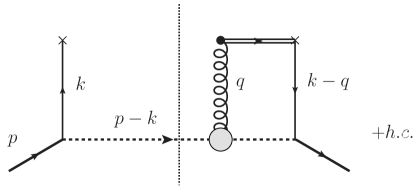
Figure 2: Cut diagram contributing to the average transverse-momentum of T-odd effects in single spin asymmetries of a SIDIS process, in the $A^{+}=0$ gauge and for a proton target described in a quark-diquark model.

V Conclusions

In this work, we have investigated the origin of nontrivial relations between transverse distortions in the distribution of quarks in impact-parameter space and analogous distortions in transverse-momentum space. The former are encoded in impact-parameter distributions (IPDs) and contribute to observable asymmetries in exclusive processes involving hadrons. The latter are encoded in the T-odd Sivers and Boer-Mulders transverse-momentum distributions (TMDs), and give rise to observable asymmetries in semi-inclusive processes involving hadrons.

We have identified the conditions under which it is possible to express the Sivers and Boer-Mulders functions as convolutions of an IPD and a lensing function, incorporating the effects of the FSIs between the active parton and the rest of the hadron. These conditions, listed in Sec. I, appear to be very specific and hold in a restricted class of models.

To better illustrate the nature of these conditions, we checked the validity or failure of the lensing relation in three models: (1) a model of the pion described as a quark-antiquark bound state, (2) a model of the proton as a bound state of three quarks, and (3) a model of the proton as a bound state of a quark and a spectator. The conditions of validity of the lensing relation are more easily fulfilled in models where the hadron is described as a two-body bound system, as in models (1) and (3). However, they can be violated even in these simple models, as happens in certain versions of (3), e.g., with axial-vector spectators that admit longitudinal polarization. Finally, the conditions are violated in model (2) and in general can not be obtained if the hadron is described by more than two constituents and the interaction vertex of the gauge boson occurs with a single constituent.

In conclusion, it seems that the lensing relation is unlikely to survive in the full complexity of nonperturbative QCD, even approximately. Phenomenological studies of the Sivers and Boer-Mulders function, as well as possible lattice QCD studies, should be able to confirm the violation of the lensing hypothesis.

Appendix A

In this appendix we explicitly derive the conditions 1) – 4) on the matrix elements of the FSI operator discussed in Sec. (I). Condition 1) follows from the requirement that the IPD we want to factorize in Eq. (27) is diagonal in the parton Fock space. Analogously, condition 2) is necessary to recover the correct Fourier transform of the quark fields that enters the definition of the IPD correlator. Conditions 3) and 4) are a consequence of momentum conservation. The matrix element of the function $I^{i}(l)$ in Eq. (28) connects states with total momenta given by

$$\bm{{W}_{\perp}}=\sum_{i=1}^{n}\bm{{w}}_{\perp,i}, \quad W^{+}=\sum_{i=1}^{n}w^{+}_{i},$$

$$\bm{{Q}_{\perp}}=\sum_{i=1}^{n}\bm{{q}}_{\perp,i}, \quad Q^{+}=\sum_{i=1}^{n}q^{+}_{i}.$$ (69)

By imposing total momentum conservation in each matrix elements of Eq. (27), we have

$$\bm{{Q}_{\perp}}=\bm{{W}_{\perp}}+\bm{{l}_{\perp}},\quad Q^{+}=W^{+}=(1-x)p^{+}.$$ (70)

Eqs. (69) and (70) are equivalent to

$$\sum_{i=1}^{n}\bm{{q}}_{\perp,i}=\sum_{i=1}^{n}\bm{{w}}_{\perp,i}+\bm{{l}_{\perp}},\quad\sum_{i=1}^{n}\frac{q^{+}_{i}}{p^{+}}=\sum_{i=1}^{n}\frac{w^{+}_{i}}{p^{+}}=\sum_{i=1}^{n}x_{i}=1-x.$$ (71)

Combining the two relations in Eq. (71), we find

$$\bm{{q}}_{\perp,i}=\bm{{w}}_{\perp,i}+\frac{x_{i}}{1-x}\bm{{l}_{\perp}}.$$ (72)

As final result, the conditions 1) – 4) can be recast in the expression of Eq. (28) for the matrix element of the lensing function. By inserting Eq. (28) in Eq. (27), we have

$$\begin{split}\braket{k_{\perp}^{i}(x)}_{UT}&=\frac{1}{2}\int\{dk_{1}\}\{dk_{2}\}\frac{d\bm{{l}_{\perp}}}{(2\pi)^{2}}\int\frac{dz^{-}}{2\pi}e^{ixp^{+}z^{-}}e^{-i\frac{z^{-}}{2}(k^{+}_{1}+k^{+}_{2})}\sum_{n}\sum_{\beta}\int\prod_{i=1}^{m}\frac{dw^{+}_{i}d\bm{w}_{\perp,i}}{(2\pi)^{3}2w_{i}^{+}}\\ &\quad\times L^{i}\left(\frac{\bm{{l}_{\perp}}}{1-x}\right)\braket{p^{+},\bm{{0}}_{\perp},\bm{{S}}_{\perp}}{\phi(k_{1})\gamma^{+}}{\left\{w^{+}_{i},\bm{w}_{\perp,i}+x_{i}\frac{\bm{{l}_{\perp}}}{1-x}\right\}_{m}}\braket{\{w^{+}_{i},\bm{w}_{\perp,i}\}_{m}}{\psi(k_{2})}{p^{+},\bm{{0}}_{\perp},\bm{{S}}_{\perp}}.\end{split}$$ (73)

We now use the invariance of the matrix elements in Eq. (73) under transverse light-front boosts to obtain

$$\braket{k_{\perp}^{i}(x)}_{UT} =\frac{1}{2}\int\{dk_{1}\}\{dk_{2}\}\frac{d\bm{{l}_{\perp}}}{(2\pi)^{2}}\int\frac{dz^{-}}{2\pi}e^{ixp^{+}z^{-}}e^{-i\frac{z^{-}}{2}(k^{+}_{1}+k^{+}_{2})}\sum_{n}\sum_{\beta}\int\prod_{i=1}^{m}\frac{dw^{+}_{i}d\bm{w}_{\perp,i}}{(2\pi)^{3}2w_{i}^{+}}$$

$$\quad\times L^{i}\left(\frac{\bm{{l}_{\perp}}}{1-x}\right)\braket{p^{+},-\bm{{l}_{\perp}},\bm{{S}}_{\perp}}{\phi(z_{1})\gamma^{+}}{\{w^{+}_{i},\bm{w}_{\perp,i}\}_{m}}\braket{\{w^{+}_{i},\bm{w}_{\perp,i}\}_{m}}{\psi(z_{2})}{p^{+},\bm{{0}}_{\perp},\bm{{S}}_{\perp}}$$

$$=\frac{1}{2}\int\frac{d\bm{{l}_{\perp}}}{(2\pi)^{2}}\int\frac{dz^{-}}{2\pi}e^{ixp^{+}z^{-}}L^{i}\left(\frac{\bm{{l}_{\perp}}}{1-x}\right)\braket{p^{+},-\bm{{l}_{\perp}},\bm{{S}}_{\perp}}{\phi(k_{1})\gamma^{+}\psi(k_{2})}{p^{+},\bm{{0}}_{\perp},\bm{{S}}_{\perp}}.$$ (74)

Eq. (74) can be finally Fourier transformed in the impact parameter space, with the result

$$\braket{k_{\perp}^{i}(x)}_{UT} =\frac{1}{2}\int\frac{d\bm{{l}_{\perp}}}{(2\pi)^{2}}\int\frac{dz^{-}}{2\pi}e^{ixp^{+}z^{-}}\int d\bm{{b}_{\perp}}e^{-i\bm{{b}_{\perp}}\bm{{l}_{\perp}}}L^{i}\left(\frac{\bm{{l}_{\perp}}}{1-x}\right)\braket{p^{+},\bm{{R}}_{\perp}=\bm{{0}_{\perp}},\bm{{S}}_{\perp}}{\phi(z_{1})\gamma^{+}\psi(z_{2})}{p^{+},\bm{{R}}_{\perp}=\bm{{0}_{\perp}},\bm{{S}}_{\perp}}$$

$$=\frac{1}{2}\int\frac{dz^{-}}{2\pi}e^{ixp^{+}z^{-}}\int d\bm{{b}_{\perp}}\mathcal{L}^{i}\left(\frac{\bm{{b}_{\perp}}}{1-x}\right)\braket{P^{+},\bm{{R}}_{\perp}=\bm{{0}_{\perp}},\bm{{S}}_{\perp}}{\phi(z_{1})\gamma^{+}\psi(z_{2})}{P^{+},\bm{{R}}_{\perp}=\bm{{0}_{\perp}},\bm{{S}}_{\perp}},$$ (75)

where we recognize the convolution of the lensing function $\mathcal{L}(\bm{{b}_{\perp}}/(1-x))$ and the correlator for unpolarized quark in a transversely polarized target that is related the IPD $\left(\mathcal{E}(x,\bm{{b}_{\perp}}^{2})\right)^{\prime}$, i.e.

$$\braket{k_{\perp}^{i}(x)}_{UT} =\int d\bm{{b}_{\perp}}\mathcal{L}^{i}\left(\frac{\bm{{b}_{\perp}}}{1-x}\right)\frac{\epsilon_{\perp}^{jk}b^{j}_{\perp}S^{k}_{\perp}}{M}\left(\mathcal{E}(x,\bm{{b}_{\perp}}^{2})\right)^{\prime}.$$ (76)

References

References

- Meissner et al. (2008) S. Meissner, A. Metz, M. Schlegel, and K. Goeke, JHEP 08, 038 (2008), arXiv:0805.3165 [hep-ph] .
- Meissner et al. (2009) S. Meissner, A. Metz, and M. Schlegel, JHEP 08, 056 (2009), arXiv:0906.5323 [hep-ph] .
- Lorcé and Pasquini (2013) C. Lorcé and B. Pasquini, JHEP 09, 138 (2013), arXiv:1307.4497 [hep-ph] .
- Lorcé et al. (2011) C. Lorcé, B. Pasquini, and M. Vanderhaeghen, JHEP 05, 041 (2011), arXiv:1102.4704 [hep-ph] .
- Burkardt and Pasquini (2016) M. Burkardt and B. Pasquini, Eur. Phys. J. A52, 161 (2016), arXiv:1510.02567 [hep-ph] .
- Diehl and Hagler (2005) M. Diehl and P. Hagler, Eur. Phys. J. C44, 87 (2005), arXiv:hep-ph/0504175 [hep-ph] .
- Meissner et al. (2007) S. Meissner, A. Metz, and K. Goeke, Phys. Rev. D76, 034002 (2007), arXiv:hep-ph/0703176 [HEP-PH] .
- Avakian et al. (2010) H. Avakian, A. V. Efremov, P. Schweitzer, and F. Yuan, Phys. Rev. D81, 074035 (2010), arXiv:1001.5467 [hep-ph] .
- Burkardt (2002) M. Burkardt, Phys. Rev. D66, 114005 (2002), arXiv:hep-ph/0209179 [hep-ph] .
- Burkardt (2004a) M. Burkardt, Nucl. Phys. A735, 185 (2004a), arXiv:hep-ph/0302144 [hep-ph] .
- Burkardt and Hwang (2004) M. Burkardt and D. S. Hwang, Phys. Rev. D69, 074032 (2004), arXiv:hep-ph/0309072 [hep-ph] .
- Bacchetta et al. (2008) A. Bacchetta, F. Conti, and M. Radici, Phys. Rev. D78, 074010 (2008), arXiv:0807.0323 [hep-ph] .
- Bacchetta and Radici (2011) A. Bacchetta and M. Radici, Phys. Rev. Lett. 107, 212001 (2011), arXiv:1107.5755 [hep-ph] .
- Burkardt (2005) M. Burkardt, Phys. Rev. D72, 094020 (2005), arXiv:hep-ph/0505189 [hep-ph] .
- Burkardt and Hannafious (2008) M. Burkardt and B. Hannafious, Phys. Lett. B658, 130 (2008), arXiv:0705.1573 [hep-ph] .
- Gamberg and Schlegel (2010) L. Gamberg and M. Schlegel, Phys. Lett. B685, 95 (2010), arXiv:0911.1964 [hep-ph] .
- Pasquini and Yuan (2010) B. Pasquini and F. Yuan, Phys. Rev. D81, 114013 (2010), arXiv:1001.5398 [hep-ph] .
- Pasquini et al. (2008) B. Pasquini, S. Cazzaniga, and S. Boffi, Phys. Rev. D78, 034025 (2008), arXiv:0806.2298 [hep-ph] .
- Boffi et al. (2003) S. Boffi, B. Pasquini, and M. Traini, Nucl. Phys. B649, 243 (2003), arXiv:hep-ph/0207340 [hep-ph] .
- Pasquini et al. (2005) B. Pasquini, M. Pincetti, and S. Boffi, Phys. Rev. D72, 094029 (2005), arXiv:hep-ph/0510376 [hep-ph] .
- Pasquini and Boffi (2007) B. Pasquini and S. Boffi, Phys. Lett. B653, 23 (2007), arXiv:0705.4345 [hep-ph] .
- Collins (2002) J. C. Collins, Phys. Lett. B536, 43 (2002), arXiv:hep-ph/0204004 [hep-ph] .
- Collins and Soper (1982) J. C. Collins and D. E. Soper, Nucl. Phys. B194, 445 (1982).
- Ji and Yuan (2002) X.-d. Ji and F. Yuan, Phys. Lett. B543, 66 (2002), arXiv:hep-ph/0206057 [hep-ph] .
- Belitsky et al. (2003) A. V. Belitsky, X. Ji, and F. Yuan, Nucl. Phys. B656, 165 (2003), arXiv:hep-ph/0208038 [hep-ph] .
- Boer et al. (2003) D. Boer, P. J. Mulders, and F. Pijlman, Nucl. Phys. B667, 201 (2003), arXiv:hep-ph/0303034 [hep-ph] .
- Sivers (1990) D. W. Sivers, Phys. Rev. D41, 83 (1990).
- Sivers (1991) D. W. Sivers, Phys. Rev. D43, 261 (1991).
- Boer and Mulders (1998) D. Boer and P. J. Mulders, Phys. Rev. D57, 5780 (1998), arXiv:hep-ph/9711485 [hep-ph] .
- Burkardt (2000) M. Burkardt, Phys. Rev. D62, 071503 (2000), [Erratum: Phys. Rev.D66,119903(2002)], arXiv:hep-ph/0005108 [hep-ph] .
- Burkardt (2003) M. Burkardt, Int. J. Mod. Phys. A18, 173 (2003), arXiv:hep-ph/0207047 [hep-ph] .
- Soper (1977) D. E. Soper, Phys. Rev. D15, 1141 (1977).
- Boer et al. (1998) D. Boer, P. J. Mulders, and O. V. Teryaev, Phys. Rev. D57, 3057 (1998), arXiv:hep-ph/9710223 [hep-ph] .
- Kanazawa and Koike (2000) Y. Kanazawa and Y. Koike, Phys. Lett. B478, 121 (2000), arXiv:hep-ph/0001021 [hep-ph] .
- Eguchi et al. (2007) H. Eguchi, Y. Koike, and K. Tanaka, Nucl. Phys. B763, 198 (2007), arXiv:hep-ph/0610314 [hep-ph] .
- Kanazawa et al. (2015) K. Kanazawa, A. Metz, D. Pitonyak, and M. Schlegel, Phys. Lett. B742, 340 (2015), arXiv:1411.6459 [hep-ph] .
- Kanazawa et al. (2016) K. Kanazawa, Y. Koike, A. Metz, D. Pitonyak, and M. Schlegel, Phys. Rev. D93, 054024 (2016), arXiv:1512.07233 [hep-ph] .
- Qiu and Sterman (1991) J.-w. Qiu and G. F. Sterman, Phys. Rev. Lett. 67, 2264 (1991).
- Burkardt (2004b) M. Burkardt, Phys. Rev. D69, 057501 (2004b), arXiv:hep-ph/0311013 [hep-ph] .
- Diehl et al. (2001) M. Diehl, T. Feldmann, R. Jakob, and P. Kroll, Nucl. Phys. B596, 33 (2001), [Erratum: Nucl. Phys.B605,647(2001)], arXiv:hep-ph/0009255 [hep-ph] .
- Ji et al. (2004) X.-d. Ji, J.-P. Ma, and F. Yuan, Eur. Phys. J. C33, 75 (2004), arXiv:hep-ph/0304107 [hep-ph] .
- Brodsky et al. (2010) S. J. Brodsky, B. Pasquini, B.-W. Xiao, and F. Yuan, Phys. Lett. B687, 327 (2010), arXiv:1001.1163 [hep-ph] .
- Pasquini and Schweitzer (2014) B. Pasquini and P. Schweitzer, Phys. Rev. D90, 014050 (2014), arXiv:1406.2056 [hep-ph] .
- Lorcé and Pasquini (2011) C. Lorcé and B. Pasquini, Phys. Rev. D84, 034039 (2011), arXiv:1104.5651 [hep-ph] .