Non-Hermitian Dynamic Strings and Anomalous Topological Degeneracy on non-Hermitian Toric-code Model with Parity-time Symmetry

Abstract

In this paper, with the help of Hermitian/non-Hermitian dynamic strings, the theory of non-Hermitian topological order is developed based on a non-Hermitian Wen-plaquette model. The effective models for bosonic topological excitations (e-particle and m-particle) are Hermitian tight-binding lattice model; the effective model for fermionic topological excitation (f-particle) becomes a non-Hermitian tight-binding lattice model. In addition, the effective pseudo-spin model for topologically degenerate ground states is derived by calculating the expectation values of Hermitian/non-Hermitian topological closed dynamic strings. For the topologically degenerate ground states of non-Hermitian Wen-plaquette model on an even-by-odd, odd-by-even and odd-by-odd lattice, anomalous topological degeneracy occurs, i.e., the number of the topologically protected ground states may be reduced from $2$ to $1$. Now, the effective pseudo-spin model turns into the typical $\mathcal{PT}$-symmetric non-Hermitian Hamiltonian with spontaneous $\mathcal{PT}$-symmetry breaking. At “exceptional points”, the topologically degenerate ground states merge with each other and the topological degeneracy turns into non-Hermitian degeneracy. In the end, the application of the non-Hermitian $Z_{2}$ topological order and its possible physics realization are discussed.

I Introduction

The non-Hermitian Hamiltonians obeying Parity-time ($\mathcal{PT}$)-symmetry as a complex extension of the (Hermitian) quantum mechanics can exist purely real energy spectrum, which was proposed by Bender and BoettcherBender 98 . It can exists spontaneous $\mathcal{PT}$-symmetry breaking accompanied by spectral transition from real to complex. The energy degeneracy points in non-Hermitian system are called “exceptional points” (EPs), at which energies coalesce and eigenvectors merge with each other. In physics, $\mathcal{PT}$-symmetric non-Hermitian systems are always obtained by appropriately engineered gain and loss. There are a variety of suitable platforms to realize $\mathcal{PT}$-symmetric non-Hermitian systems, such as opticsGuo2009 ; Ruter2010 ; Chong2011 ; Regensburger2012 ; Feng2013 ; Wimmer2015 ; Weimann2017 ; Hodaei2017 ; Ozdemir2019 , electronicsSchindler2011 ; Assawaworrarit2017 ; Choi2018 , microwavesBittner2012 ; Peng2014 ; Poli2015 ; Liu2016 , acousticsZhuX2014 ; Popa2014 ; Fleury2015 ; Ding2016 , single-spin systemWu2019 , and dynamic systemsXiao2017 ; luo ; Xiao2019 ; Wang2019 . Some applications associated with $\mathcal{PT}$-symmetric system have been explored including unidirectional transportFeng2013 ; Peng2014 and single-mode lasersFeng2014 ; Hodaei2014 .

On the other hand, the non-Hermitian topological states and topological invariants of tight-binding models have been widely studiedRudner2009 ; Esaki2011 ; Hu2011 ; Liang2013 ; Zhu2014 ; Lee2016 ; San2016 ; Leykam2017 ; Shen2018 ; Lieu2018 ; Xiong2018 ; Kawabata2018 ; Gong2018 ; Yao2018 ; YaoWang2018 ; Yin2018 ; Kunst2018 ; KawabataUeda2018 ; Alvarez2018 ; Jiang2018 ; Ghatak2019 ; Avila2019 ; Jin2019 ; Lee2019 ; Liu2019 ; 38-1 ; 38 ; chen-class2019 ; Edvardsson2019 ; Herviou2019 ; Yokomizo2019 ; zhouBin2019 ; Kunst2019 ; Deng2019 ; SongWang2019 ; xi2019 ; Longhi2019 ; chen-edge2019 . The classification of non-Hermitian topological phases in terms of symmetries has been developed including $\mathcal{PT}$-symmetryGong2018 ; 38-1 ; 38 . However, there exists another type of topological states beyond Landau’s symmetry breaking paradigm – topological orderswen3 . For the topological orders, all the excitations are gapped and have fractional statistics and the ground states have topological degeneracy, i.e., the quantum degeneracy of the ground states depends on the genius of the manifold of the backgroundwen3 ; k1 ; k2 ; wen1 ; wen2 ; kou1 ; kou2 ; kou3 ; md . The degenerate ground states of a topological order (on a torus) make up a protected code subspace (the topological qubits). It is possible to incorporate intrinsic fault tolerance into a quantum computer - topological quantum computation (TQC) which avoids decoherence and is free from errorsk1 ; k2 .

A question is ”How about topological orders meet $\mathcal{PT}$-symmetric non-Hermitian?” In this paper, by taking the non-Hermitian Wen-plaquette (toric-code) model as an example, we will study a $Z_{2}$ topological order on a $\mathcal{PT}$ symmetric non-Hermitian system and develop a theory for non-Hermitian ($Z_{2}$) topological order. The quantum states of non-Hermitian Wen-plaquette (toric-code) are characterized by Hermitian/non-Hermitian dynamic strings. The topological degeneracy for the system on even-by-odd, odd-by-even and odd-by-odd lattices becomes anomalous: the topologically degenerate ground states may merge with each other and the topological degeneracy turns into non-Hermitian degeneracy. The number of the topologically protected ground states turns to $1$ rather than $2$. We call it anomalous topological degeneracy.

In this paper, we will develop a theory of the non-Hermitian $Z_{2}$ topological order by taking the Wen-plaquette model as an example. The remainder of the paper is organized as follows. In Sec. II, we review the theory of Hermitian $Z_{2}$ topological order (the Wen-plaquette model). In Sec. III, a non-Hermitian Wen-plaquette model is proposed. In Sec. IV, based on biorthogonal set, the theory for non-Hermitian quantum string states in the non-Hermitian $Z_{2}$ topological order is developed. In Sec. V, the propertities of quasi-particles in the non-Hermitian $Z_{2}$ topological order is given. The effective model for fermionic quasi-particles is non-Hermitian and the energy spectra become complex. In Sec. VI, the physics of anomalous topological degeneracy are explored. The effective model for the degenerate ground states on even-by-odd, odd-by-even and odd-by-odd lattices is derived that always has $\mathcal{PT}$-symmetry. In this section, spontaneous $\mathcal{PT}$-symmetry breaking for the topologically protected degenerate ground states is discovered. The numerical results confirm the analytic theoretical predictions. Finally, the conclusions are given in Sec. VII.

II $Z_{2}$ topological order for Hermitian Wen-plaquette model

Firstly, we review the topological properties of (Hermitian) $Z_{2}$ topological order. There are several exactly solvable spin models with $Z_{2}$ topological orders, such as the Kitaev toric-code model k1 , the Wen-plaquette model wen1 ; wen2 and the Kitaev model on a honeycomb lattice k2 . In this paper, we take Wen-plaquette model as an example.

II.1 The (Hermitian) Wen-plaquette model

The Hamiltonian of the (Hermitian) Wen-plaquette modelwen3 ; k1 ; k2 ; wen1 ; wen2 is

$$\hat{H}=-g\sum_{i}\hat{F}_{i},$$ (1)

with

$$F_{i}=\sigma_{i}^{x}\sigma_{i+\hat{e}_{x}}^{y}\sigma_{i+\hat{e}_{x}+\hat{e}_{y}}^{x}\sigma_{i+\hat{e}_{y}}^{y},$$ (2)

and $g>0.$ $\sigma_{i}^{x},$ $\sigma_{i}^{y}$ are Pauli matrices on site $i$. In this paper, $g$ is set to be unit, $g\equiv 1$. In Fig.1, we show the schematic diagram of the (Hermitian) Wen-plaquette model. The ground state is a topological order described by $Z_{2}$ gauge symmetry that is denoted by ${F_{i}\equiv+1}$ at each plaquette with the ground state energy

$$E_{0}=-g\mathcal{N},$$ (3)

where $\mathcal{N}$ is the total lattice numberwen1 ; wen2 .

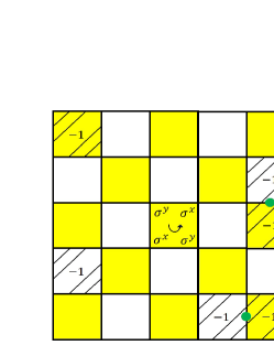
Figure 1: (Color online) The schematic diagram of the (Hermitian) Wen-plaquette model. The yellow/white plaquette stands for odd/even sub-plaquette, respectively. The shadow region in odd/even sub-plaquette represent an m-particle and e-particle, respectively. Green spheres on the links represent f-particles.

II.2 (Hermitian) quantum string states

The quantum states of the (Hermitian) Wen-plaquette model are characterized by different configurations of stringswen3 ; k1 ; k2 ; wen1 ; wen2 ,

$$\left|\Phi\right\rangle=\sum_{\mathcal{C}}a_{\mathcal{C}}\hat{W}(\mathcal{C})|0\rangle,$$ (4)

where $\hat{W}(\mathcal{C})=\prod_{\mathcal{C}}\sigma_{i}^{\alpha_{i}}$ denote the possible open/closed string operators, and $a_{\mathcal{C}}$ is weight of the string operator. $\sigma_{i}^{\alpha_{i}}$ is $\alpha_{i}$-type Pauli matrix on site $i$ and $\prod_{i\in\mathcal{C}}$ is over all the sites on the string along a loop $\mathcal{C}$, and, where $|0\rangle$ denotes the spin polarized states with all spin down ($\left|\downarrow\downarrow,\cdots,\downarrow\right\rangle$). Here, the string operators are all Hermitian, i.e.,

$$\hat{W}(\mathcal{C})=\hat{W}^{\dagger}(\mathcal{C}),$$ (5)

and for quantum string states we have

$$\hat{W}(\mathcal{C})\left|\Phi\right\rangle=\hat{W}^{\dagger}(\mathcal{C})\left|\Phi\right\rangle=d(\mathcal{C})\left|\Phi\right\rangle,$$ (6)

where $d(\mathcal{C})$ is eigenvalue and $\left|\Phi\right\rangle$ is the eigenstate. For example, the ground state is an equal superposition of loop (closed string) configurations: $\sum_{\mathcal{C}\in\mathrm{closed-string}}\hat{W}(\mathcal{C})|0\rangle$. The closed loops are interpreted as electric field lines of the $Z_{2}$ gauge theory. On a torus, the ground states have topological degeneracy, of which the wave-functions are characterized by topological closed strings.

II.3 Energy spectra of quasi-particles

In the Wen-plaquette model, there are three types of quasi-particles, e-particle (or $Z_{2}$ charge), m-particle (or $Z_{2}$ vortex), and f-particle (or fermion). m-particle is defined as ${F_{i}=-1}$ at odd sub-plaquette and e-particle is defined as ${F_{i}=-1}$ at even sub-plaquette. The mass gap of e-particle and m-particle is $2g$. In particular, the bound states of an e-particle and an m-particle on two neighbor plaquettes are f-particle obeying fermionic statistic. See the illustration in Fig.1. All quasi-particles in such exactly solvable model can’t move. The energy spectra are $E_{v}=E_{c}=2g$ for e-particle and m-particle, $E_{f}=4g$ for fermion, respectively.

These three types of quasi-particles (e-particle, m-particle, and f-particle) can be characterized by three types of (open) string operators $W_{c}(\mathcal{C})$, $W_{v}(\mathcal{C})$, $W_{f}(\mathcal{C})$ that are all Hermitian,

$$W_{c}(\mathcal{C}) =W_{c}^{\dagger}(\mathcal{C}),\text{ }W_{v}(\mathcal{C})=W_{v}^{\dagger}(\mathcal{C}),$$

$$W_{f}(\mathcal{C}) =W_{f}^{\dagger}(\mathcal{C}).$$ (7)

For each open string, the corresponding quantum states are two excited quasi-particles. The string operator for a pair of e-particles $W_{c}(\mathcal{C})=\prod_{\mathcal{C}}\sigma_{i}^{\alpha_{i}}$ (or a pair of m-particles $W_{v}(\mathcal{C})=\prod_{\tilde{\mathcal{C}}}\sigma_{i}^{\alpha_{i}}$) is the product of spin operators along a loop $\mathcal{C}$ (or $\tilde{\mathcal{C}}$) connecting adjacent even-plaquettes (or odd-plaquettes), $\alpha_{i}=y$ if $i$ is even and $\alpha_{i}=x$ if $i$ is odd. The string for a pair of f-particles described by the $W_{f}(\mathcal{C})=W_{c}(\mathcal{C})W_{v}(\mathcal{C})$ can be regarded as a combination of the string for e-particles and m-particles.

It was known that for the Wen-plaquette model, the quasi-particles cannot move in the solvable limit. The situation changes after adding external fields. Under the perturbation $H_{I}=h_{x}\sum\limits_{i}\sigma_{i}^{x}+h_{z}\sum\limits_{i}\sigma_{i}^{z},$ the quasi-particles (e-particle, m-particle and f-particle) begin to hop. The term $h_{x}\sum\limits_{i}\sigma_{i}^{x}$ drives the e-particle, m-particle and f-particle hopping along diagonal direction $\hat{e}_{x}-\hat{e}_{y}$, and the term $h_{z}\sum\limits_{i}\sigma_{i}^{z}$ drive f-particle hopping along $\hat{e}_{x}$ or $\hat{e}_{y}$ direction without affecting e-particle and m-particle. There exist two types of f-particles: the f-particles on the vertical links and the f-particles on the parallel links. The term $h_{z}\sum\limits_{i}\sigma_{i}^{z}$ drives the f-particles on the vertical links move along vertical directions and the f-particles on the parallel links move along parallel directions. That means both types of f-particle cannot turn round any more under the term $h_{z}\sum\limits_{i}\sigma_{i}^{z}$. But these two types of f-particles can be converted into each other under the term $h_{x}\sum\limits_{i}\sigma_{i}^{x}$, as has been shown in Fig.2.

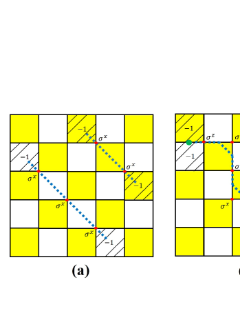
Figure 2: (Color online) (a) The schematic diagram of strings for e/m-particle under the term $\hat{H}_{I}$; (b) The schematic diagram of strings for f-particle under the term $\hat{H}_{I}$.

Let us calculate the energy spectra for three types of quasi-particles.

For an e-particle (or m-particle) living at $i$ plaquette ${F_{i}=-1,}$ when $\sigma^{x}$ acts on $i+\hat{e}_{x}$ site, it hops to $i+\hat{e}_{x}-\hat{e}_{y}$ plaquette denoted by ${F_{i+\hat{e}_{x}-\hat{e}_{y}}=-1}$. Moreover, a pair of e-particles (or m-particles) located at $i$ and $i+\hat{e}_{x}-\hat{e}_{y}$ plaquettes can be created by the operator of $\sigma_{i+\hat{e}_{x}}^{x}$,

$${F_{i}} {=}{+1\rightarrow F_{i}=-1,}$$

$${F_{i+\hat{e}_{x}-\hat{e}_{y}}} {=}{+1\rightarrow F_{i+\hat{e}_{x}-\hat{e}_{y}}=-1},$$ (8)

or annihilated also

$${F_{i}} {=}{-1\rightarrow F_{i}=+1,}$$

$$F{{}_{i+\hat{e}_{x}-\hat{e}_{y}}} {=}{-1\rightarrow F_{i+\hat{e}_{x}-\hat{e}_{y}}=+1.}$$ (9)

With the help of perturbative method, each hopping term $\hat{t}_{I^{a}J^{a}}^{a}$ for e/m-particle on $I^{a}$-lattice ($a=v$ on lattice of odd sub-plaquettes and $a=c$ on lattice of even sub-plaquettes) corresponds to a one-step Hermitian string operator $\hat{t}_{i}^{a}=h_{x}\sigma_{i}^{x}$,

$$\hat{t}_{i}^{a} =h_{x}\sigma_{i}^{x}\rightarrow$$

$$\hat{t}_{I^{a}J^{a}}^{a} =h_{x}(\phi_{a,I^{a}}^{{\dagger}}\phi_{a,I^{a}+e_{x^{I^{a}}}^{I^{a}}}+\phi_{a,I^{a}}^{{\dagger}}\phi_{a,I^{a}+e_{x^{I^{a}}}^{I^{a}}}^{{\dagger}}+h.c.),$$ (10)

where $\phi_{a,I^{a}}^{{\dagger}}$ is the generation operator of the e/m-particle. Here, $e_{x^{I^{a}}}^{I^{a}}$ is the unit vector along $x^{I^{a}}$ direction on $I^{a}$-lattice, of which the lattice constant is $\sqrt{2}a_{0}$ ($a_{0}$ is lattice constant of the original square lattice). See the illustration in Fig.3(a).

The effective Hamiltonian of boson $\hat{H}_{\mathrm{eff}}^{a}$ ($a=v$ denote m-particle, $a=c$ denote e-particle) on $L_{x}\times L_{y}$ square lattice can be expressed as

$$\hat{H}_{\mathrm{eff}}^{a}= \sum_{\left\langle I^{a},J^{a}\right\rangle}h_{x}(\phi_{a,I}^{{\dagger}}\phi_{a,I^{a}+e_{x^{I^{a}}}^{I^{a}}}+\phi_{a,I}^{{\dagger}}\phi_{a,I^{a}+e_{x^{I^{a}}}^{I^{a}}}^{{\dagger}}+h.c.)$$

$$+2g\sum_{I^{a}}\phi_{a,I^{a}}^{{\dagger}}\phi_{a,I^{a}}.$$ (11)

After Fourier transformation, $\hat{H}_{\mathrm{eff}}^{a}$ is written as

$$\hat{H}_{\mathrm{eff}}^{a}=\sum_{k_{x}^{a}}\left(\begin{array}[c]{cc}\phi_{k_{x}^{a}}^{\dagger}&\phi_{-k_{x}^{a}}\end{array}\right)\mathcal{\hat{H}}_{\mathrm{eff}}^{a}\left(\begin{array}[c]{c}\phi_{k_{x}^{a}}\\ \phi_{-k_{x}^{a}}^{\dagger}\end{array}\right)-(2g+2h_{x}\cos k_{x}^{a}),$$ (12)

where $\mathcal{\hat{H}}_{\mathrm{eff}}^{a}$ in momentum space is obtained as

$$\mathcal{\hat{H}}_{\mathrm{eff}}^{a}=\left(\begin{array}[c]{cc}2g+2h_{x}\cos k_{x}^{a}&2h_{x}\cos k_{x}^{a}\\ 2h_{x}\cos k_{x}^{a}&2g+2h_{x}\cos k_{x}^{a}\end{array}\right).$$ (13)

Then we use Bogoliubov transformation,

$$\phi_{k_{x}^{a}} =u\alpha+v\beta^{\dagger},\text{ }\phi_{k_{x}^{a}}^{\dagger}=u\alpha^{\dagger}+v\beta,$$

$$\phi_{-k_{x}^{a}}^{\dagger} =v\alpha+u\beta^{\dagger},\text{ }\phi_{-k_{x}^{a}}=v\alpha^{\dagger}+u\beta,$$ (14)

where $u$ and $v$ satisfy the following conditions

$$u^{2} =\frac{1}{2}+\frac{2g+2h_{x}\cos k_{x}^{a}}{2E_{k^{a}}},$$

$$v^{2} =-\frac{1}{2}+\frac{2g+2h_{x}\cos k_{x}^{a}}{2E_{k^{a}}},$$

$$uv =-\frac{2h^{x}\cos k_{x}^{a}}{2E_{k^{a}}}.$$ (15)

Finally, the effective Hamiltonian of e-particle (or m-particle) is obtained as

$$\mathcal{\hat{H}}_{\mathrm{eff}}^{a}=\sum_{k_{x}^{a}}E_{k^{a}}(\alpha_{k_{x}^{a}}^{\dagger}\alpha_{k_{x}^{a}}+\beta_{k_{x}^{a}}^{\dagger}\beta_{k_{x}^{a}}).$$ (16)

where the energy spectra are real as

$$E_{k^{a}}=2g\sqrt{1+\frac{2h_{x}\cos k_{x}^{a}}{g}}.$$ (17)

When the term $h_{x}$ becomes larger, the energy gap for e/m-particle closes and a quantum phase transition from $Z_{2}$ topological order to spin polarized order occurs. In Fig.3(b), we plot the energy spectra of e/m-particle for the (Hermitian) Wen-plaquette model with $h_{x}=0.2$, $h_{z}=0.01$.

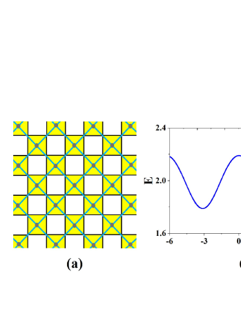
Figure 3: (Color online) (a) The schematic diagram of effective lattice for m-particle. The grey dots denote the lattice sites; (b) The energy spectra of boson for the (Hermitian) Wen-plaquette model with $h_{x}=0.2$, $h_{z}=0.01$.

On the other hand, with the help of perturbative method, the hopping term $\hat{t}_{I^{f}J^{f}}^{f}$ for two types of f-particles on $I^{f}$-lattice (lattice of links) corresponds to a one-step string operator $\hat{t}_{i}^{f}=h_{x}\sigma_{i}^{x}+h_{z}\sigma_{i}^{z}$, i.e.,

$$\hat{t}_{i}^{f} =h_{x}\sigma_{i}^{x}+h_{z}\sigma_{i}^{z}$$

$$\rightarrow\hat{t}_{I^{f}J^{f}}^{f}=h_{x}(\phi_{f_{1},I^{f}}^{{\dagger}}\phi_{f_{2},I^{f}+e_{x^{I^{f}}}^{I^{f}}}+\phi_{f_{1},I^{f}}^{{\dagger}}\phi_{f_{2},I^{f}+e_{x^{I^{f}}}^{I^{f}}}^{{\dagger}}$$

$$+\phi_{f_{1},I^{f}}^{{\dagger}}\phi_{f_{2},I^{f}-e_{x^{I^{f}}}^{I^{f}}}+\phi_{f_{1},I^{f}}^{{\dagger}}\phi_{f_{2},I^{f}-e_{x^{I^{f}}}^{I^{f}}}^{{\dagger}}+h.c.)$$

$$+h_{z}(\phi_{f_{1},I^{f}}^{{\dagger}}\phi_{f_{1},I^{f}+(e_{x^{I^{f}}}^{I^{f}}+e_{y^{I^{f}}}^{I^{f}})}+\phi_{f_{1},I^{f}}^{{\dagger}}\phi_{f_{1},I^{f}+(e_{x^{I^{f}}}^{I^{f}}+e_{y^{I^{f}}}^{I^{f}})}^{{\dagger}}$$

$$+\phi_{f_{2},I^{f}}^{{\dagger}}\phi_{f_{2},I^{f}+(e_{x^{I^{f}}}^{I^{f}}-e_{y^{I^{f}}}^{I^{f}})}+\phi_{f_{2},I^{f}}^{{\dagger}}\phi_{f_{2},I^{f}+(e_{x^{I^{f}}}^{I^{f}}-e_{y^{I^{f}}}^{I^{f}})}^{\dagger}$$

$$+h.c.),$$ (18)

where $\phi_{f_{1},I^{f}}^{{\dagger}}$ and $\phi_{f_{2},I^{f}}^{{\dagger}}$ are the generation operator of the f-particles on two sub-links, respectively. Here, $e_{x^{I^{f}}}^{I^{f}}$ and $e_{y^{I^{f}}}^{I^{f}}$ are the unit vector along $x^{I^{f}}$ and $y^{I^{f}}$ direction on $I^{f}$-lattice, respectively, with lattice constant to be $\frac{\sqrt{2}}{2}a_{0}$. See the illustration in Fig.4(a).

Then, the effective Hamiltonian of f-particle is obtained as

$$\hat{H}_{\mathrm{eff}}^{f}= \sum_{\langle I^{f},J^{f}\rangle}h_{x}\big{[}(\phi_{f_{1},I^{f}}^{{\dagger}}\phi_{f_{2},I^{f}+e_{x^{I^{f}}}^{I^{f}}}+\phi_{f_{1},I^{f}}^{{\dagger}}\phi_{f_{2},I^{f}+e_{x^{I^{f}}}^{I^{f}}}^{{\dagger}}$$

$$+\phi_{f_{1},I^{f}}^{{\dagger}}\phi_{f_{2},I^{f}-e_{x^{I^{f}}}^{I^{f}}}+\phi_{f_{1},I^{f}}^{{\dagger}}\phi_{f_{2},I^{f}-e_{x^{I^{f}}}^{I^{f}}}^{{\dagger}})+h.c.\big{]}$$

$$+\sum_{\langle I^{f},J^{f}\rangle}h_{z}\big{[}(\phi_{f_{1},I^{f}}^{{\dagger}}\phi_{f_{1},I^{f}+(e_{x^{I^{f}}}^{I^{f}}+e_{y^{I^{f}}}^{I^{f}})}$$

$$+\phi_{f_{1},I^{f}}^{{\dagger}}\phi_{f_{1},I^{f}+(e_{x^{I^{f}}}^{I^{f}}+e_{y^{I^{f}}}^{I^{f}})}^{{\dagger}}+\phi_{f_{2},I^{f}}^{{\dagger}}\phi_{f_{2},I^{f}+(e_{x^{I^{f}}}^{I^{f}}-e_{y^{I^{f}}}^{I^{f}})}$$

$$+\phi_{f_{2},I^{f}}^{{\dagger}}\phi_{f_{2},I^{f}+(e_{x^{I^{f}}}^{I^{f}}-e_{y^{I^{f}}}^{I^{f}})}^{\dagger}+h.c.\big{]}$$

$$+4g\sum_{I^{f}}\phi_{f_{1},I^{f}}^{{\dagger}}\phi_{f_{1},I^{f}}+4g\sum_{I^{f}}\phi_{f_{2},I^{f}}^{{\dagger}}\phi_{f_{2},I^{f}}.$$ (19)

After Fourier transformation, $\hat{H}_{\mathrm{eff}}^{f}$ can be written as

$$\hat{H}_{\mathrm{eff}}^{f}=\left(\begin{array}[c]{cccc}\phi_{ok}^{\dagger}&\phi_{o-k}&\phi_{ek}^{\dagger}&\phi_{e-k}\end{array}\right)\hat{\mathcal{H}}_{\mathrm{eff}}^{f}\left(\begin{array}[c]{c}\phi_{ok}\\ \phi_{o-k}^{\dagger}\\ \phi_{ek}\\ \phi_{e-k}^{\dagger}\end{array}\right),$$ (20)

where the effective Hamiltonian $\mathcal{\hat{H}}_{\mathrm{eff}}^{f}$ in momentum space is obtained as

$$\hat{\mathcal{H}}_{\mathrm{eff}}^{f}=\left(\begin{array}[c]{cccc}4g+A_{1}&iB_{1}&C&C\\ -iB_{1}&-4g-A_{1}&-C&-C\\ C&-C&4g+A_{2}&iB_{2}\\ C&-C&-iB_{2}&-4g-A_{2}\end{array}\right),$$ (21)

with $A_{1}=2h_{z}\cos(k_{x}^{f}+k_{y}^{f})$, $A_{2}=2h_{z}\cos(k_{x}^{f}-k_{y}^{f})$, $B_{1}=2h_{z}\sin(k_{x}^{f}+k_{y}^{f})$, $B_{2}=2h_{z}\sin(k_{x}^{f}-k_{y}^{f})$, $C=2h_{x}\cos k_{x}^{f}$. In Fig.4(b), we plot the energy spectra of f-particle for the (Hermitian) Wen-plaquette model with $h_{x}=0.2$, $h_{z}=0.01$.

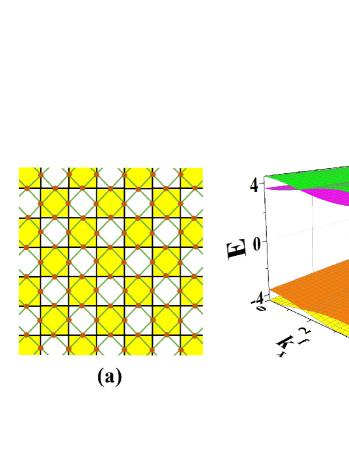
Figure 4: (Color online) (a) The schematic diagram of effective lattice for f-particle. The red dots denote the lattice sites; (b) The energy spectra of fermion for the (Hermitian) Wen-plaquette model with $h_{x}=0.2$, $h_{z}=0.01$.

II.4 Degenerate ground states

In this part, we review the degeneracy of ground states $\mathcal{D}$ for the Wen-plaquette model. Under the periodic boundary condition (on a torus), the degeneracy $\mathcal{D}$ is dependent on lattice number: $\mathcal{D}=4$ on even-by-even ($e\ast e$) lattice, $\mathcal{D}=2$ on other cases (even-by-odd ($e\ast o$), odd-by-even ($o\ast e$) and odd-by-odd ($o\ast o$) lattices)wen3 ; k1 ; k2 ; wen1 ; wen2 ; kou1 ; kou2 .

To classify the degeneracy of the ground states of $Z_{2}$ topological order, we define topological closed string operators around torus.

For the Wen-plaquette model on an $e\ast e$ lattice, there are four types of topological closed string operators, $W_{v}(\mathcal{C}_{X}),$ $W_{v}(\mathcal{C}_{Y}),$ $W_{f}(\mathcal{C}_{X})$ and $W_{f}(\mathcal{C}_{Y}).$ Here $\mathcal{C}_{X}$ denotes a topological closed loop around the torus along x-direction and $C_{Y}$ denotes a topological closed loop around the torus along y-direction. The four types of topological closed string operators are all Hermitian, i.e.,

$$W_{v}(\mathcal{C}_{X}) =W_{v}^{\dagger}(\mathcal{C}_{X}),\text{ }W_{v}(\mathcal{C}_{Y})=W_{v}^{\dagger}(\mathcal{C}_{Y}),$$

$$W_{f}(\mathcal{C}_{X}) =W_{f}^{\dagger}(\mathcal{C}_{X}),\text{ }W_{f}(\mathcal{C}_{Y})=W_{f}^{\dagger}(\mathcal{C}_{Y}).$$ (22)

Due to the commutation and anti-commutation relations between $W_{v}(\mathcal{C}_{A})$ and $W_{f}(\mathcal{C}_{B})$, $\left\{W_{v}(\mathcal{C}_{X}),W_{f}(\mathcal{C}_{Y})\right\}=0,$ $\left[W_{v}(\mathcal{C}_{X}),W_{f}(\mathcal{C}_{X})\right]=0,$ $\left\{W_{v}(\mathcal{C}_{Y}),W_{f}(\mathcal{C}_{X})\right\}=0,$ $\left[W_{v}(\mathcal{C}_{Y}),W_{f}(\mathcal{C}_{Y})\right]=0,$ we may represent $W_{v}(\mathcal{C}_{X}),$ $W_{v}(\mathcal{C}_{Y}),$ $W_{f}(\mathcal{C}_{X})$ and $W_{f}(\mathcal{C}_{Y})$ by pseudo-spin operators $\tau_{1}^{x},$ $\tau_{2}^{x},$ $\tau_{2}^{z}$ and $\tau_{1}^{z}$, respectively. The ground states becomes the eigenstates of $\tau_{l}^{z}$ ($l=1,2$). Then one has four degenerate ground states (denoted by $|m_{1},m_{2}\rangle=|m_{1}\rangle\otimes|m_{2}\rangle$). For $m_{l}=0,$ we have $\tau_{l}^{z}|m_{l}\rangle=|m_{l}\rangle,$ and for $m_{l}=1$ we have $\tau_{l}^{z}|m_{l}\rangle=-|m_{l}\rangle.$ Physically, the topological degeneracy arises from the presence or absence of $\pi$ flux of fermion through the hole. The values of $m_{l}$ reflect the presence ($m_{l}=1$) or the absence ($m_{l}=0$) of the $\pi$ flux in the hole. A ground state becomes the linear combination of the four degenerate ground states $\left|0\right\rangle=\displaystyle\sum_{m_{1},m_{2}=0,1}\alpha_{m_{1},m_{2}}|m_{1},m_{2}\rangle$, where $\alpha_{m_{1},m_{2}}$ is the weight of $|m_{1},m_{2}\rangle$.

Similarly we may use the closed string operators to describe the ground states on $e\ast o$ lattice, $o\ast e$ lattice and $o\ast o$ lattice. For example, for the Wen-plaquette model on an $e\ast o$ lattice, we can only define two types of topological closed string operators, $W_{v}(\mathcal{C}_{X})$ and $W_{f}(\mathcal{C}_{Y}).$ There is no topological closed string operator for m-particles along y-direction with odd number of lattices. Due to the anti-commutation relations between, $W_{v}(\mathcal{C}_{X})$ and $W_{f}(\mathcal{C}_{Y})$, $\left\{W_{v}(\mathcal{C}_{X}),W_{f}(\mathcal{C}_{Y})\right\}=0,$ we may represent $W_{v}(\mathcal{C}_{X})$ and $W_{f}(\mathcal{C}_{Y})$ by pseudo-spin operators $\tau^{x}$ and $\tau^{z}$, respectively. The ground states becomes the eigenstates of $\tau^{z}$. Then one has two degenerate ground states (denoted by $|m\rangle$). For $m=0,$ we have $\tau^{z}|m\rangle=|m\rangle,$ and for $m=1$ we have $\tau^{z}|m\rangle=-|m\rangle.$

It is known that the degenerate ground states of $Z_{2}$ topological orders have same energy in thermodynamic limit. However, in a finite system,  the degeneracy of the ground states is (partially) removed due to tunneling processes, of which a virtual quasi-particle moves around the torus before annihilating with the other onek1 ; kou1 ; kou2 . For example, at first a pair of the m-particle is created. One of the m-particles propagates all the way around the torus and then annihilates with the other m-particle. Such a process effectively adds a unit of the $\pi$-flux to the hole of the torus and changes $m_{a}$ or $m_{b}$ by $1$. To characterize the low energy effective physics of degenerate ground states, we derive the effective (Hermitian) pseudo-spin Hamiltonian of the degenerate ground states.

III Non-Hermitian Wen-plaquette model with $\mathcal{PT}$-symmetry

We introduce a non-Hermitian Wen-plaquette (toric-code) model with $\mathcal{PT}$-symmetry, of which the Hamiltonian is

$$\hat{H}_{\mathrm{NTO}}=\hat{H}_{\mathrm{TO}}+\hat{H}_{\mathrm{PT}},$$ (23)

where

$$\hat{H}_{\mathrm{TO}}=-{g\sum_{i}F_{i}},$$ (24)

with ${F_{i}=\sigma_{i}^{x}\sigma_{i+\hat{e}_{x}}^{y}\sigma_{i+\hat{e}_{x}+\hat{e}_{y}}^{x}\sigma_{i+\hat{e}_{y}}^{y}}$ and

$$\hat{H}_{\mathrm{PT}}={\sum\limits_{i}}(h_{x}\sigma_{i}^{x}+ih_{z}\sigma_{i}^{z}),$$ (25)

$h_{x},h_{z}$ are two real parameters. $\sigma_{i}^{x,y,z}$ are Pauli matrices on sites $i$.

We define parity operator $\mathcal{P}$ and time-reversal operator$\ \mathcal{T}$, i.e., the time reversal operator $\mathcal{T}$ has the function

$$\mathcal{T}i\mathcal{T=-}i,$$ (26)

and the parity operator $\mathcal{P}$ has the function of rotating each spin by $\pi$ about the $x$-axis

$$\mathcal{P}={\displaystyle\prod\limits_{j=1}^{N}}\sigma_{j}^{x}.$$ (27)

As a result, the Hamiltonian $\hat{H}_{\mathrm{NTO}}$ is $\mathcal{PT}$ invariant

$$\left[\mathcal{P},\hat{H}_{\mathrm{NTO}}\right]\neq 0\text{ and }\left[\mathcal{T},\hat{H}_{\mathrm{NTO}}\right]\neq 0,$$ (28)

but

$$\left[\mathcal{PT},\text{ }\hat{H}_{\mathrm{NTO}}\right]=0.$$

For the case of $g\gg h_{x},h_{z}$, $\hat{H}_{\mathrm{NTO}}\rightarrow\hat{H}_{\mathrm{TO}},$ we have a $Z_{2}$ topological ordered state. In this limit, the elementary excitations (m/e-particles) are defined as ${F_{i}=-1}$ at odd/even sub-plaquette. The bound states of an e-particle and a m-particle obey fermionic statistic. For the case of $g\ll h_{x},h_{z}$, $\hat{H}_{\mathrm{NTO}}\rightarrow\hat{H}_{\mathrm{PT}}$, we have a typical non-Hermitian Hamiltonian with spontaneous $\mathcal{PT}$-symmetry breaking.

In this paper, we focus on the case of $g\gg h_{x},h_{z}$ and treat the non-Hermitian term $\hat{H}_{\mathrm{PT}}$ as a perturbation. Now, the ground state becomes a non-Hermitian $Z_{2}$ topological ordered state.

IV Biorthogonal description for non-Hermitian dynamic strings

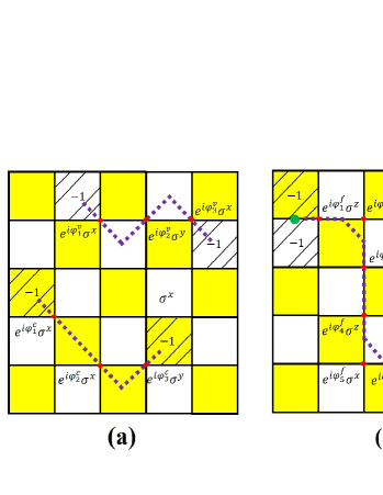
Figure 5: (Color online) (a) The schematic diagram of dynamic strings for e/m-particles under the perturbation; (b) The schematic diagram of dynamic strings for f-particle under the perturbation.

IV.1 Dynamic strings for the non-Hermitian $Z_{2}$ topological order

To characterize the quantum properties of the non-Hermitian topological order for $\hat{H}_{\mathrm{NTO}}$, we introduce three types of strings along a $N$-step loop $\mathcal{C}_{N}$: the operation strings $W_{a}(\mathcal{C}_{N})$, the phase strings $P_{a}(\mathcal{C}_{N})$, and the dynamic strings $D_{a}(\mathcal{C}_{N})$, respectively. The indices $a=v,$ $c,$ $f$ correspond to three types of quasi-particles.

An operation string is defined as the product of spin operators,

$$W_{a}(\mathcal{C}_{N})=\prod_{i\in C}\sigma_{i}^{\alpha_{i}},$$ (29)

where $\prod_{i\in\mathcal{C}}$ is over all the sites on the string along a loop $\mathcal{C}$. $\sigma_{i}^{\alpha_{i}}$ is $\alpha_{i}$-type Pauli matrix on site $i$. A phase string is introduced as the product of phases along a loop $\mathcal{C},$

$$P_{a}(\mathcal{C}_{N})=\prod_{i\in C}e^{i\varphi_{i}^{a}},$$ (30)

where $\varphi_{i}^{a}$ is the phase of the quantum states at step $i$ for $a$-type excitation. The dynamic string $D_{a}(\mathcal{C}_{N})$ is introduced to characterize the hopping property, i.e.,

$$D_{a}(\mathcal{C}_{N})=\prod_{i\in\mathcal{C}}\frac{\hat{t}_{i}^{a}}{\left|\hat{t}_{i}^{a}\right|},$$ (31)

where

$$\frac{\hat{t}_{i}^{a}}{\left|\hat{t}_{i}^{a}\right|}=e^{i\varphi_{i}^{a}}\sigma_{i}^{\alpha_{i}}.$$ (32)

For a given topological excitation ($a=v,$ $c,$ or $f$), a dynamic string is a combination of an operation string and a phase string, according to the relationship of the three types of strings, i.e.,

$$D_{a}(\mathcal{C}_{N})=W_{a}(\mathcal{C}_{N})P_{a}(\mathcal{C}_{N}).$$ (33)

The phase strings $P_{a}(\mathcal{C}_{N})$ and the dynamic strings $D_{a}(\mathcal{C}_{N})$ can be Hermitian or non-Hermitian. We then define Hermitian/non-Hermitian dynamic string $D_{a}(\mathcal{C}_{N})$ by verifying its conjugation. For the case of

$$D_{a}(\mathcal{C}_{N})=D_{a}^{\dagger}(\mathcal{C}_{N}),$$ (34)

a dynamic string is Hermitian; For the case of

$$D_{a}(\mathcal{C}_{N})\neq D_{a}^{\dagger}(\mathcal{C}_{N}),$$ (35)

a dynamic string is non-Hermitian.

IV.2 Biorthogonal set for the quantum string states

To characterize the non-Hermitian dynamic string $D_{a}(\mathcal{C}_{N})\neq D_{a}^{\dagger}(\mathcal{C}_{N})$, we introduce the biorthogonal set for the quantum string states of the non-Hermitian $Z_{2}$ topological orderma .

In general, for non-Hermitian dynamic strings, we define left/right eigenstates defined as

$$D_{a}(\mathcal{C}_{N})|{\Psi}^{\mathrm{R}}\rangle=d_{a}(\mathcal{C}_{N})|{\Psi}^{\mathrm{R}}\rangle,$$ (36)

and

$$D_{a}^{\dagger}(\mathcal{C}_{N})|{\Psi}^{\mathrm{L}}\rangle=d_{a}^{\ast}(\mathcal{C}_{N})|{\Psi}^{\mathrm{L}}\rangle,$$ (37)

where $d_{a}(\mathcal{C}_{N})$, $d_{a}^{\ast}(\mathcal{C}_{N})$ are the corresponding eigenvalues. The eigenstates can be bi-orthogonalized as

$$|\widetilde{{\Psi}}_{n}^{\mathrm{R}}\rangle=|{\Psi}_{n}^{\mathrm{R}}\rangle/\sqrt{\langle{\Psi}_{n}^{\mathrm{L}}|{\Psi}_{n}^{\mathrm{R}}\rangle},$$ (38)

and

$$|\widetilde{{\Psi}}_{n}^{\mathrm{L}}\rangle=|{\Psi}_{n}^{\mathrm{L}}\rangle/\sqrt{\langle{\Psi}_{n}^{\mathrm{R}}|{\Psi}_{n}^{\mathrm{L}}\rangle},$$ (39)

which then gives

$$\langle{\widetilde{\Psi}}_{n}^{\mathrm{L}}|\widetilde{{\Psi}}_{m}^{\mathrm{R}}\rangle=\delta_{nm},$$ (40)

and

$$\sum_{n}|{\widetilde{\Psi}}_{m}^{\mathrm{R}}\rangle\langle{\widetilde{\Psi}}_{n}^{\mathrm{L}}|=1.$$ (41)

As a result, we have

$$D_{a}^{\dagger}(\mathcal{C}_{N})|\widetilde{\Psi}_{n}^{\mathrm{R}}\rangle=d_{a}(\mathcal{C}_{N})|\widetilde{\Psi}_{n}^{\mathrm{R}}\rangle.$$ (42)

In particular, a dynamic string is $\mathcal{PT}$-symmetric non-Hermitian when it satisfies the following conditions,

$$\left[\mathcal{P},D_{a}(\mathcal{C}_{N})\right]\neq 0,~{}~{}\left[\mathcal{T},D_{a}(\mathcal{C}_{N})\right]\neq 0,$$ (43)

but

$$\left[\mathcal{PT},\text{ }D_{a}(\mathcal{C}_{N})\right]=0.$$ (44)

IV.3 Dynamic strings for non-Hermitian Wen-plaquette model

For the non-Hermitian topological order described by $\hat{H}_{\mathrm{NTO}},$ we show the detailed definitions for three types of strings.

To create an e-particle/m-particle, one define the operation string that connects the nearest neighboring even (odd) sub-plaquettes

$$W_{c/v}(\mathcal{C}_{N})=\prod_{i\in\mathcal{C}}\sigma_{i}^{\alpha_{i}}.$$ (45)

The product $\prod_{i\in\mathcal{C}}$ is over all the sites on the string along a loop $\mathcal{C}$ connecting even-plaquettes (or odd-plaquettes), $\alpha_{i}=x$ if $i$ is odd and $\alpha_{i}=y$ if $i$ is even. Under the perturbation $h_{x}{\displaystyle\sum\limits_{i}}\sigma_{i}^{x},$ the e-particle/m-particle begins to hop along $\hat{e}_{x}-\hat{e}_{y}$ direction. As a result, we have $\hat{t}_{i}^{v/c}=h_{x}\sigma_{i}^{x}.$ The phase string and dynamic string for e-particle/m-particle are obtained as

$$P_{c}(\mathcal{C}_{N}) =P_{v}(\mathcal{C}_{N})=1,$$

$$D_{c}(\mathcal{C}_{N}) =D_{v}(\mathcal{C}_{N})=\prod_{i\in\mathcal{C}}\sigma_{i}^{x},$$ (46)

respectively.

The operation string for f-particles is defined as

$$W_{f}(\mathcal{C}_{N})=\prod_{i\in\mathcal{C}}\sigma_{i}^{\alpha_{i}},$$ (47)

where $\alpha_{i}=z$ if the string does not turn at site $i$, $\alpha_{i}=x$ if the turn forms a upper-left or lower-right corner, $\alpha_{i}=y$ if the turn forms a lower-left or upper-right corner. Under a perturbation $ih_{z}\sum\limits_{i}\sigma_{i}^{z}$, f-particles begin to move. Now, we have $\hat{t}_{i}^{f}=ih_{z}\sigma_{i}^{z}$ (without considering the term $h_{x}{\displaystyle\sum\limits_{i}}\sigma_{i}^{x}$). The phase string and dynamic string for fermion are obtained as

$$P_{f}(\mathcal{C}_{N}) =\prod_{i\in\mathcal{C}}e^{i\varphi_{i}^{a}},$$

$$D_{f}(\mathcal{C}_{N}) =\prod_{i\in\mathcal{C}}e^{i\varphi_{i}^{a}}\sigma_{i}^{z}.$$ (48)

with $\varphi_{i}^{a}=\frac{\pi}{2}$. For the case of even number $N$, the phase string is $P_{f}(\mathcal{C}_{N})=\pm 1$ and the dynamic string is

$$D_{f}(\mathcal{C}_{N})=\pm\prod_{i\in\mathcal{C}}\sigma_{i}^{z}=\pm W_{f}(\mathcal{C}_{N}).$$ (49)

The phase string and dynamic string for fermions are Hermitian($D_{f}^{{\dagger}}(\mathcal{C}_{N})=D_{f}(\mathcal{C}_{N})$). For the case of odd number $N$, the phase string is $P_{f}(\mathcal{C}_{N})=e^{\pm i\frac{\pi}{2}}$ and the dynamic string is

$$D_{f}(\mathcal{C}_{N})=e^{\pm i\frac{\pi}{2}}\prod_{i\in\mathcal{C}}\sigma_{i}^{z}=e^{\pm i\frac{\pi}{2}}W_{f}(\mathcal{C}_{N}),$$ (50)

that is $\mathcal{PT}$-symmetric non-Hermitian according to

$$\left[\mathcal{P},D_{f}(\mathcal{C}_{N})\right]\neq 0,\text{ }\left[\mathcal{T},D_{f}(\mathcal{C}_{N})\right]\neq 0,$$ (51)

and

$$\left[\mathcal{PT},\text{ }D_{f}(\mathcal{C}_{N})\right]=0.$$ (52)

V Quasi-particles

The open string creates two point-like objects that correspond to different types of quasi-particles (topological excitations) at its ends. In this part, we use the perturbative method to describe the effective Hamiltonian of quasi-particles. These effective Hamiltonians describe a hard-core boson/fermion system.

V.1 Energy spectra for e/m-particle

By perturbative method, each hopping term $\hat{t}_{I^{a}J^{a}}^{a}$ for e/m-particle on $I^{a}$-lattice ($a=v$ on lattice of odd sub-plaquettes and $a=c$ on lattice of even sub-plaquettes) corresponds to a one-step Hermitian dynamic string

$$\hat{t}_{i}^{a} =h_{x}\sigma_{i}^{x}\rightarrow\hat{t}_{I^{a}J^{a}}^{a}=h_{x}(\phi_{a,I^{a}}^{{\dagger}}\phi_{a,I^{a}+e_{x^{I^{a}}}^{I^{a}}}$$

$$+\phi_{a,I^{a}}^{{\dagger}}\phi_{a,I^{a}+e_{x^{I^{a}}}^{I^{a}}}^{{\dagger}}+h.c.),$$ (53)

where $\phi_{a,I^{a}}^{{\dagger}}$ is the generation operator of the e/m-particle. Here, $e_{x^{I^{a}}}^{I^{a}}$ is the unit vector along $x^{I^{a}}$ direction on $I^{a}$-lattice, of which the lattice constant is $\sqrt{2}a_{0}$ ($a_{0}$ is lattice constant of the original square lattice).

The perturbative effective Hamiltonian of boson $\hat{H}_{\mathrm{eff}}^{a}$ ($a=v$ denote vortex excitation, $a=c$ denote charge excitation) on $L_{x}\times L_{y}$ square lattice can be expressed as

$$\hat{H}_{\mathrm{eff}}^{a}= \sum_{\left\langle I^{a},J^{a}\right\rangle}h_{x}(\phi_{a,I}^{{\dagger}}\phi_{a,I^{a}+e_{x^{I^{a}}}^{I^{a}}}+\phi_{a,I}^{{\dagger}}\phi_{a,I^{a}+e_{x^{I^{a}}}^{I^{a}}}^{{\dagger}}+h.c.)$$

$$+2g\sum_{I^{a}}\phi_{a,I^{a}}^{{\dagger}}\phi_{a,I^{a}}.$$ (54)

The effective Hamiltonian $\mathcal{\hat{H}}_{\mathrm{eff}}^{a}$ in momentum space of e/m-particle can be obtained as $\mathcal{\hat{H}}_{\mathrm{eff}}^{a}=\sum_{k_{x}^{a}}E_{k^{a}}(\alpha_{k_{x}^{a}}^{\dagger}\alpha_{k_{x}^{a}}+\beta_{k_{x}^{a}}^{\dagger}\beta_{k_{x}^{a}})$ where the energy spectra can be expressed as

$$E_{k^{a}}=\sqrt{(2g+2h_{x}\cos k_{x}^{a})^{2}-(2h^{x}\cos k_{x}^{a})^{2}}.$$ (55)

The result is same as the Hermitian case.

V.2 Non-Hermitian lattice model and complex spectra for f-particle

In the perturbative method, the hopping term $\hat{t}_{I^{f}J^{f}}^{f}$ for two types of f-particle on $I^{f}$-lattice (lattice of links) corresponds to a one-step non-Hermitian dynamic string $\hat{t}_{i}^{f}=h_{x}\sigma_{i}^{x}+ih_{z}\sigma_{i}^{z}$, i.e.,

$$\hat{t}_{i}^{f} =h_{x}\sigma_{i}^{x}+ih_{z}\sigma_{i}^{z}$$

$$\rightarrow\hat{t}_{I^{f}J^{f}}^{f}=h_{x}(\phi_{f_{1},I^{f}}^{{\dagger}}\phi_{f_{2},I^{f}+e_{x^{I^{f}}}^{I^{f}}}+\phi_{f_{1},I^{f}}^{{\dagger}}\phi_{f_{2},I^{f}+e_{x^{I^{f}}}^{I^{f}}}^{{\dagger}}$$

$$+\phi_{f_{1},I^{f}}^{{\dagger}}\phi_{f_{2},I^{f}-e_{x^{I^{f}}}^{I^{f}}}+\phi_{f_{1},I^{f}}^{{\dagger}}\phi_{f_{2},I^{f}-e_{x^{I^{f}}}^{I^{f}}}^{{\dagger}}+h.c.)$$

$$+ih_{z}(\phi_{f_{1},I^{f}}^{{\dagger}}\phi_{f_{1},I^{f}+(e_{x^{I^{f}}}^{I^{f}}+e_{y^{I^{f}}}^{I^{f}})}+\phi_{f_{1},I^{f}}^{{\dagger}}\phi_{f_{1},I^{f}+(e_{x^{I^{f}}}^{I^{f}}+e_{y^{I^{f}}}^{I^{f}})}^{{\dagger}}$$

$$+\phi_{f_{2},I^{f}}^{{\dagger}}\phi_{f_{2},I^{f}+(e_{x^{I^{f}}}^{I^{f}}-e_{y^{I^{f}}}^{I^{f}})}+\phi_{f_{2},I^{f}}^{{\dagger}}\phi_{f_{2},I^{f}+(e_{x^{I^{f}}}^{I^{f}}-e_{y^{I^{f}}}^{I^{f}})}^{\dagger}$$

$$+h.c.),$$ (56)

where $\phi_{f_{1},I^{f}}^{{\dagger}}$ and $\phi_{f_{2},I^{f}}^{{\dagger}}$ are the generation operator of the fermionic quasi-particles on two sub-links, respectively. Here, $e_{x^{I^{f}}}^{I^{f}}$ and $e_{y^{I^{f}}}^{I^{f}}$ are the unit vector along $x^{I^{f}}$ and $y^{I^{f}}$ direction on $I^{f}$-lattice, respectively, with lattice constant to be $\frac{\sqrt{2}}{2}a_{0}$. In particular, the hopping term $\hat{t}_{I^{f}J^{f}}^{f}=h_{x}\sigma_{i}^{x}+ih_{z}\sigma_{i}^{z}$ corresponding to a one-step non-Hermitian dynamic string becomes non-Hermitian, i.e., $\hat{t}_{I^{f}J^{f}}^{f}\neq(\hat{t}_{I^{f}J^{f}}^{f})^{\dagger}$.

Consequently, the perturbative effective Hamiltonian of f-particle becomes non-Hermitian that is obtained as

$$\hat{H}_{\mathrm{eff}}^{f}= \sum_{\langle I^{f},J^{f}\rangle}h_{x}\big{[}(\phi_{f_{1},I^{f}}^{{\dagger}}\phi_{f_{2},I^{f}+e_{x^{I^{f}}}^{I^{f}}}+\phi_{f_{1},I^{f}}^{{\dagger}}\phi_{f_{2},I^{f}+e_{x^{I^{f}}}^{I^{f}}}^{{\dagger}}$$

$$+\phi_{f_{1},I^{f}}^{{\dagger}}\phi_{f_{2},I^{f}-e_{x^{I^{f}}}^{I^{f}}}+\phi_{f_{1},I^{f}}^{{\dagger}}\phi_{f_{2},I^{f}-e_{x^{I^{f}}}^{I^{f}}}^{{\dagger}})+h.c.\big{]}$$

$$+\sum_{\langle I^{f},J^{f}\rangle}ih_{z}\big{[}(\phi_{f_{1},I^{f}}^{{\dagger}}\phi_{f_{1},I^{f}+(e_{x^{I^{f}}}^{I^{f}}+e_{y^{I^{f}}}^{I^{f}})}$$

$$+\phi_{f_{1},I^{f}}^{{\dagger}}\phi_{f_{1},I^{f}+(e_{x^{I^{f}}}^{I^{f}}+e_{y^{I^{f}}}^{I^{f}})}^{{\dagger}}+\phi_{f_{2},I^{f}}^{{\dagger}}\phi_{f_{2},I^{f}+(e_{x^{I^{f}}}^{I^{f}}-e_{y^{I^{f}}}^{I^{f}})}$$

$$+\phi_{f_{2},I^{f}}^{{\dagger}}\phi_{f_{2},I^{f}+(e_{x^{I^{f}}}^{I^{f}}-e_{y^{I^{f}}}^{I^{f}})}^{\dagger}+h.c.\big{]}$$

$$+4g\sum_{I^{f}}\phi_{f_{1},I^{f}}^{{\dagger}}\phi_{f_{1},I^{f}}+4g\sum_{I^{f}}\phi_{f_{2},I^{f}}^{{\dagger}}\phi_{f_{2},I^{f}}.$$ (57)

After Fourier transformation, the effective Hamiltonian $\hat{H}_{\mathrm{eff}}^{f}$ can be written as

$$\hat{H}_{\mathrm{eff}}^{f}=\left(\begin{array}[c]{cccc}\phi_{ok}^{\dagger}&\phi_{o-k}&\phi_{ek}^{\dagger}&\phi_{e-k}\end{array}\right)\hat{\mathcal{H}}_{\mathrm{eff}}^{f}\left(\begin{array}[c]{c}\phi_{ok}\\ \phi_{o-k}^{\dagger}\\ \phi_{ek}\\ \phi_{e-k}^{\dagger}\end{array}\right),$$ (58)

where the effective Hamiltonian $\mathcal{\hat{H}}_{\mathrm{eff}}^{f}$ in momentum space is obtained as

$$\hat{\mathcal{H}}_{\mathrm{eff}}^{f}=\left(\begin{array}[c]{cccc}4g+iA_{1}&-B_{1}&C&C\\ B_{1}&-4g-iA_{1}&-C&-C\\ C&-C&4g+iA_{2}&-B_{2}\\ C&-C&B_{2}&-4g-iA_{2}\end{array}\right)$$ (59)

with

$$A_{1} =2h_{z}\cos(k_{x}^{f}+k_{y}^{f}),\text{ }A_{2}=2h_{z}\cos(k_{x}^{f}-k_{y}^{f}),$$

$$B_{1} =2h_{z}\sin(k_{x}^{f}+k_{y}^{f}),\text{ }B_{2}=2h_{z}\sin(k_{x}^{f}-k_{y}^{f}),$$

$$C =2h_{x}\cos k_{x}^{f}.$$ (60)

As a result, the Hamiltonian $\mathcal{\hat{H}}_{\mathrm{eff}}^{f}$ can be rewritten as

$$\mathcal{\hat{H}}_{\mathrm{eff}}^{f} =4g(\mathbb{I\otimes}{\tau^{z})}+\frac{1}{2}iA_{1}(\mathbb{I\otimes}{\tau^{z}+\sigma^{z}\otimes\tau^{z})}$$

$$+\frac{1}{2}iA_{2}(\mathbb{I\otimes}{\tau^{z}-{\sigma^{z}}\otimes\tau^{z})}$$

$$+\frac{1}{2}B_{1}\mathbf{(}-\mathbb{I\otimes}i{\tau^{y}-{\sigma^{z}}\otimes i\tau^{y})}$$

$$+\frac{1}{2}B_{2}\mathbf{(}-\mathbb{I\otimes}i{\tau^{y}+{\sigma^{z}}\otimes i\tau^{y})}$$

$$+C({{\sigma^{x}}\otimes\tau^{z}-{\sigma^{y}}\otimes\tau^{y})},$$ (61)

where ${\sigma^{i},}$ ${\tau^{i}}$ $(i=x,y,z)$ are Pauli matrices, $\mathbb{I}$ is a $2\times 2$ identity matrix.

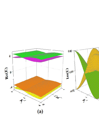
Figure 6: (Color online) (a) The real part of energy spectrum of f-particle for the non-Hermitian Wen-plaquette model with $h_{x}=0.2$, $h_{z}=0.01;$ (b) The imaginary part of energy spectrum of fermion for the non-Hermitian Wen-plaquette model with $h_{x}=0.2$, $h_{z}=0.01.$

By diagonalizing this Hamiltonian, we can obtain the energy spectra for f-particles that are tedious. Therefore, we focus on some special points in momentum space. For example, at $k_{x}^{f}=\pm\frac{\pi}{2},$ $k_{y}^{f}=0$, the effective Hamiltonian is reduced into

$$\hat{H}_{\mathrm{eff}}^{f}=4g(\mathbb{I\otimes}{\tau^{z})}\pm 2ih_{z}{(}\mathbb{I\otimes}{\tau^{y}).}$$ (62)

The corresponding energy spectrum turns into

$$E_{\mathrm{eff}}^{f}=\pm\sqrt{\left(4g\right)^{2}-\left(2h_{z}\right)^{2}}.$$ (63)

A $\mathcal{PT}$-symmetry-breaking transition occurs at the exceptional points $E_{\mathrm{eff}}^{f}=0$ that leads to the following relation $2g=h_{z}.$

In Fig.6, we plot the real part and imaginary part of energy spectra of f-particle for the non-Hermitian Wen-plaquette model with $h_{x}=0.2$, $h_{z}=0.01$. One can see that the energy spectra of f-particle are complex due to the non-Hermitian term, which is different from the Hermitian case.

VI Anomalous topological degeneracy

It was known that the ground state for $\hat{H}_{\mathrm{TO}}$ is a $Z_{2}$ topological order, of which the ground states have topological degeneracy, i.e., different topologically degenerate ground states are classified by different topological closed strings $W_{a}(\mathcal{C}_{N}^{\mathrm{close,topo}})$ that are all Hermitian, $W_{a}(\mathcal{C}_{N}^{\mathrm{close,topo}})=W_{a}^{\dagger}(\mathcal{C}_{N}^{\mathrm{close,topo}})$. Under the periodic boundary condition (on a torus) for $\hat{H}_{\mathrm{TO}}$, the degeneracy is dependent on lattice number, i.e., $4$ on a even-by-even ($e\ast e$) lattice, $2$ on even-by-odd ($e\ast o$), odd-by-even ($o\ast e$) and odd-by-odd ($o\ast o$) lattices. Thus we get a four-level (or two-level) system which can be mapped onto an effective pseudo-spin model for topologically degenerate ground stateskou1 ; kou2 .

After considering the non-Hermitian perturbation $\hat{H}_{\mathrm{PT}},$ the ground states are classified by different topological closed dynamic strings around the torus $D_{a}(\mathcal{C}_{N}^{\mathrm{close,topo}})$ that may be either Hermitian or non-Hermitian. Under the periodic boundary condition (on a torus) for $\hat{H}_{\mathrm{NTO}}$, the degeneracy is also dependent on lattice number, i.e., $4$ on a even-by-even ($e\ast e$) lattice, $2$ on even-by-odd ($e\ast o$), odd-by-even ($o\ast e$) and odd-by-odd ($o\ast o$) lattices. The effective model for the topologically degenerate ground states can also be mapped onto an effective pseudo-spin model. After considering the quantum tunneling processes that change one ground state to another, the transfer matrices between different topologically degenerate ground states are characterized by the expectation values of topological closed dynamic strings $D_{a}(\mathcal{C}_{N}^{\mathrm{close,topo}})$. Consequently, the effective pseudo-spin model for topologically degenerate ground states may be either Hermitian or non-Hermitian. In the following parts, we will derive the effective (Hermitian or non-Hermitian) pseudo-spin model for topologically degenerate ground states by calculating the expectation values for different topological closed dynamic strings around the torus $D_{a}(\mathcal{C}_{N}^{\mathrm{close,topo}})$.

For the case of $e\ast e$ lattice, the topological closed dynamic strings $D_{a}(\mathcal{C}_{N}^{\mathrm{close}})$ ($a=v,c$ or $f$) that correspond to different quantum tunneling processes are all Hermitian, the effective pseudo-spin model $\mathcal{\hat{H}}_{\mathrm{eff}}^{e\ast e}$ for topologically degenerate ground states is also Hermitian. Therefore, in this part we focus on the case of non-Hermitian Wen-plaquette model $\hat{H}_{\mathrm{NTO}}$ on $o\ast e$ or $e\ast o,$ $o\ast o$ lattice.

VI.1 Non-Hermitian higher Order perturbation theory

Firstly, a non-Hermitian higher order perturbation theory is developed to calculate the energy splitting of the two degenerate ground states of non-Hermitian Wen-plaquette model on $o\ast e$ or $e\ast o,$ $o\ast o$ lattice. For $m_{l}=0,$ we have $\tau_{l}^{z}|m_{l}\rangle=|m_{l}\rangle,$ and for $m_{l}=1$ we have $\tau_{l}^{z}|m_{l}\rangle=-|m_{l}\rangle.$ We denote $|0\rangle$ and $|1\rangle$ by $\mid\uparrow\rangle$ and $\left|\downarrow\right\rangle,$ respectively.

$\mid\uparrow\rangle_{R}$ and $\mid\uparrow\rangle_{L}$ is one of the ground state of $\hat{H}_{0}$ and $\hat{H}_{0}^{\dagger}$ under biorthogonal set, $\mid\downarrow\rangle_{R}$ and $\mid\downarrow\rangle_{L}$ is another ground state of $\hat{H}_{0}$ and $\hat{H}_{0}^{\dagger}$ under biorthogonal set. Under perturbation $\hat{H}_{I}$, $\hat{H}_{0}$ turns into $\hat{H}$. Now, the quantum states of $\mid\uparrow\rangle_{R}$ and $\mid\downarrow\rangle_{R}$ turn into $\left|\Phi_{\uparrow}\right\rangle_{R}$ and $\left|\Phi_{\downarrow}\right\rangle_{R}$ that can be constructed as following

$$\left|\Phi_{\uparrow}\right\rangle_{R} =\frac{\hat{U}_{I}(0,-\infty)\left|\uparrow\right\rangle_{R}}{{}_{L}\left\langle\uparrow\right|\hat{U}_{I}(0,-\infty)\left|\uparrow\right\rangle_{R}},$$ (64)

$$\left|\Phi_{\downarrow}\right\rangle_{R} =\frac{\hat{U}_{I}(0,-\infty)\left|\downarrow\right\rangle_{R}}{{}_{L}\left\langle\downarrow\right|\hat{U}_{I}(0,-\infty)\left|\downarrow\right\rangle_{R}},$$ (65)

which is the eigenstate of Hamiltonian $\hat{H}$.

The transformation operator $\hat{U_{I}}(0,-\infty)$ can be written as

$$\hat{U}_{I}(0,-\infty)=\mathrm{T}\exp(-i\int_{-\infty}^{0}\hat{H}_{I}(t)dt)$$ (66)

Here T denotes a time order and $\hat{H}_{I}(t)=e^{i\frac{\hat{H}_{0}}{\hbar}t}\hat{H}_{I}e^{-i\frac{\hat{H}_{0}}{\hbar}t}$. Then the transformation operator $\hat{U}_{I}(0,-\infty)\left|\uparrow\right\rangle_{R}$ in Eq.64 can be rewritten as

$$\hat{U}_{I}(0,-\infty)\left|\uparrow\right\rangle_{R}=\sum\limits_{j=0}^{\infty}\hat{U}_{I}^{(j)}(0,-\infty)\left|\uparrow\right\rangle_{R},$$ (67)

in which

$$\hat{U}_{I}^{(0)}(0,-\infty)\left|\uparrow\right\rangle_{R}=\left|\uparrow\right\rangle_{R}$$

and

$$\hat{U}_{I}^{(1)}(0,-\infty)\left|\uparrow\right\rangle_{R}= -\frac{i}{\hbar}\int_{-\infty}^{0}\hat{H}_{I}(t)dt\left|\uparrow\right\rangle_{R}$$

$$= \frac{1}{E_{0\uparrow}-\hat{H}_{0}}\hat{H}_{I}\left|\uparrow\right\rangle_{R},$$ (68)

and

$$\hat{U}_{I}^{(2)}(0,-\infty)\left|\uparrow\right\rangle_{R}= -\frac{i}{\hbar}\int_{-\infty}^{0}\hat{H}_{I}(t)\hat{U}_{I}^{(1)}(0,-\infty)dt\left|\uparrow\right\rangle_{R}$$

$$= \frac{1}{E_{0\uparrow}-\hat{H}}_{0}\hat{H}_{I}\frac{1}{E_{0\uparrow}-\hat{H}_{0}}\hat{H}_{I}\left|\uparrow\right\rangle_{R},$$ (69)

and

$$\hat{U}_{I}^{(j\neq 0)}(0,-\infty)\left|\uparrow\right\rangle_{R}=(\frac{1}{E_{0\uparrow}-\hat{H}_{0}}\hat{H_{I}})^{j}\left|\uparrow\right\rangle_{R}$$ (70)

where $E_{\uparrow}$ is the eigenvalue of $\left|\Phi_{\uparrow}\right\rangle_{R}$ for Hamiltonian $\hat{H}$, and $E_{0\uparrow}$ is the eigenvalue of $\left|\uparrow\right\rangle_{R}$ for Hamiltonian $\hat{H}_{0}$. Therefore, we have

$$\hat{U}_{I}(0,-\infty)\left|\uparrow\right\rangle_{R}=\left|\uparrow\right\rangle_{R}+\sum\limits_{j=1}^{\infty}(\frac{1}{E_{0\uparrow}-\hat{H}_{0}}\hat{H_{I}})^{j}\left|\uparrow\right\rangle_{R}.$$ (71)

Similarity,

$$\hat{U}_{I}(0,-\infty)\left|\downarrow\right\rangle_{R}=\left|\downarrow\right\rangle_{R}+\sum\limits_{j=1}^{\infty}(\frac{1}{E_{0\uparrow}-\hat{H}_{0}}\hat{H_{I}})^{j}\left|\downarrow\right\rangle_{R},$$ (72)

Finally, with the help of Eq.64 and Eq.65, one can get the eigenstates of Hamiltonian $\hat{H}$

$$\left|\Phi_{\uparrow}\right\rangle_{R}=\frac{\left|\uparrow\right\rangle_{R}+\sum_{j=1}^{\infty}(\frac{\hat{H_{I}}}{E_{0\uparrow}-\hat{H_{0}}})^{j}\left|\uparrow\right\rangle_{R}}{{}_{L}\left\langle\uparrow\right|\hat{U_{I}}(0,-\infty)\left|\uparrow\right\rangle_{R}},$$

$$\left|\Phi_{\downarrow}\right\rangle_{R}=\frac{\left|\downarrow\right\rangle_{R}+\sum_{j=1}^{\infty}(\frac{\hat{H_{I}}}{E_{0\uparrow}-\hat{H_{0}}})^{j}\left|\downarrow\right\rangle_{R}}{{}_{L}\left\langle\downarrow\right|\hat{U_{I}}(0,-\infty)\left|\downarrow\right\rangle_{R}}.$$

To characterize the low energy physics of topologically protected degenerate ground states, an effective edge Hamiltonian is obtained from the non-Hermitian higher order perturbation theory,

$$\mathcal{\hat{H}}_{\mathrm{eff}}=\left(\begin{array}[c]{cc}h_{\uparrow\uparrow}&h_{\uparrow\downarrow}\\ h_{\downarrow\uparrow}&h_{\downarrow\downarrow}\end{array}\right)$$ (73)

where $h_{\uparrow\uparrow}={}_{L}\left\langle\uparrow\right|\hat{H}\hat{U}_{I}(0,-\infty)\left|\uparrow\right\rangle_{R},$ $h_{\uparrow\downarrow}={}_{L}\left\langle\uparrow\right|\hat{H}\hat{U}_{I}(0,-\infty)\left|\downarrow\right\rangle_{R},$ $h_{\downarrow\uparrow}={}_{L}\left\langle\downarrow\right|\hat{H}\hat{U}_{I}(0,-\infty)\left|\uparrow\right\rangle_{R},$ and $h_{\downarrow\downarrow}={}_{L}\left\langle\downarrow\right|\hat{H}\hat{U}_{I}(0,-\infty)\left|\downarrow\right\rangle_{R}$.

VI.2 Effective non-Hermitian pseudo-spin Hamiltonian

Firstly, we study the effective pseudo-spin model for topologically degenerate ground states on an $e\ast o$ lattice that are characterized by topological closed dynamic strings around the torus $D_{a}(\mathcal{C}_{X-Y}),$ $D_{f}(\mathcal{C}_{Y})$ ($a=v$ or $c$). Here, $\mathcal{C}_{X-Y}$ denotes a dynamic string along $\hat{e}_{x}-\hat{e}_{y}$-direction and $\mathcal{C}_{Y}$ denotes a dynamic string along $\hat{e}_{y}$-direction, respectively. Due to $\left\{D_{a}(\mathcal{C}_{X-Y}),\text{ }D_{f}(\mathcal{C}_{Y})\right\}=0,$ $D_{a}(\mathcal{C}_{X-Y})$ and $D_{f}(\mathcal{C}_{Y})$ can be mapped into pseudo-spin operators $\tau^{x}$ and $\tau^{z}$, respectively. Now we map the two-fold topologically degenerate ground states $\left|m=0\right\rangle$ and $\left|m=1\right\rangle$ onto quantum states of the pseudo-spin $\tau^{z}$ as $\mid\uparrow\rangle$ and $\left|\downarrow\right\rangle$, respectively. Here, $m$ is the number of $\pi$-flux inside the holes of torus.

Under the perturbation, $\hat{H}_{\mathrm{PT}}$, there are two types of quantum tunneling processes - virtual e-particle/m-particle propagating along $\hat{e}_{x}-\hat{e}_{y}$ directions around the torus and virtual fermion propagating along $\hat{e}_{y}$ direction around the torus.

For the virtual e-particle/m-particle propagating along $\hat{e}_{x}-\hat{e}_{y}$ directions around the torus, the energy splitting $\Delta\sim{}_{L}\langle\uparrow\mid D_{c}(\mathcal{C}_{L_{0}}^{\mathrm{close,topo}})\left|\downarrow\right\rangle_{R}\sim{}_{L}\langle\downarrow\mid D_{c}(\mathcal{C}_{L_{0}}^{\mathrm{close,topo}})\left|\uparrow\right\rangle_{R}$ can be obtained by the high-order degenerate-state perturbation theory as

$$\Delta=2L_{x}L_{y}\frac{(h_{x})^{L_{0}}}{(-4g)^{L_{0}-1}},$$ (74)

where the step number $L_{0}$ is equal to

$$\frac{L_{x}L_{y}}{\xi}.$$ (75)

Here $\xi$ is the maximum common divisor for $L_{x}$ and $L_{y}$. Because the topological closed dynamic string $D_{c}(\mathcal{C}_{L_{0}}^{\mathrm{close,topo}})$ (or $D_{v}(\mathcal{C}_{L_{0}}^{\mathrm{close,topo}})$) of e-particle (or m-particle) plays a role of $\tau^{x}$ on the quantum states, we obtain the effective pseudo-spin Hamiltonian for topologically degenerate ground states due to the contribution of e-particle (or m-particle) as

$$\frac{\Delta}{2}\tau^{x};$$ (76)

For the tunneling process of f-particle propagating around the torus along direction $\hat{e}_{y}$, we obtain the energy difference

$$\varepsilon\sim{}_{L}\langle\uparrow\mid D_{f}(\mathcal{C}_{L_{y}}^{\mathrm{close,topo}})\left|\uparrow\right\rangle_{R}\sim-{}_{L}\langle\downarrow\mid D_{f}(\mathcal{C}_{L_{y}}^{\mathrm{close,topo}})\left|\downarrow\right\rangle_{R}$$ (77)

of topologically degenerate ground states as

$$\varepsilon=16L_{x}L_{y}g(\frac{ih_{z}}{8g})^{L_{y}}.$$ (78)

Because the topological closed dynamic string $D_{f}(\mathcal{C}_{L_{y}}^{\mathrm{close,topo}})$ of f-particles plays a role of $\tau^{z}$ on the quantum states, we obtain the effective pseudo-spin Hamiltonian for topologically degenerate ground states due to the contribution of f-particles as

$$\frac{\varepsilon}{2}\tau^{z}.$$ (79)

Finally, the effective pseudo-spin Hamiltonian of the two topologically degenerate ground states on an $e\ast o$ lattice is obtained as

$$\mathcal{\hat{H}}_{\mathrm{eff}}^{e\ast o}=\frac{\Delta}{2}\tau^{x}+\frac{\varepsilon}{2}\tau^{z}=\frac{1}{2}\left(\begin{array}[c]{cc}\beta(ih_{z})^{L_{y}}&\alpha h_{x}^{L_{0}}\\ \alpha h_{x}^{L_{0}}&-\beta(ih_{z})^{L_{y}}\end{array}\right)$$ (80)

where

$$\Delta=\alpha(h_{x})^{L_{0}},$$ (81)

and

$$\varepsilon=\beta(ih_{z})^{L_{y}}.$$ (82)

$\alpha$ and $\beta$ are two real parameters.

According to odd number $L_{y},$

$$\operatorname{Re}\varepsilon\equiv 0,$$ (83)

and

$$\operatorname{Im}\varepsilon=16L_{x}L_{y}g(\frac{h_{z}}{8g})^{L_{y}}\neq 0,$$ (84)

the effective pseudo-spin model $\mathcal{\hat{H}}_{\mathrm{eff}}$ turns into the typical $\mathcal{PT}$ symmetric non-Hermitian Hamiltonian that is invariant under a combined parity ($\mathcal{P}$) and time-reversal ($\mathcal{T}$) symmetry for $h_{x}$ and $g$, where $\mathcal{P}\rightarrow\tau^{x}$ simply corresponds to an exchange of the two topologically degenerate ground states and $\mathcal{T}:i\rightarrow-i$. As a result, for odd number $L_{y}$, we have

$$\left[\mathcal{P},\mathcal{\hat{H}}_{\mathrm{eff}}^{e\ast o}\right]\neq 0\text{ and }\left[\mathcal{T},\mathcal{\hat{H}}_{\mathrm{eff}}^{e\ast o}\right]\neq 0,$$ (85)

but

$$\left[\mathcal{PT},\text{ }\mathcal{\hat{H}}_{\mathrm{eff}}^{e\ast o}\right]=0.$$ (86)

We may use similar approach to get the effective non-Hermitian pseudo-spin model for topologically degenerate ground states on an $o\ast e$ lattice ($\mathcal{\hat{H}}_{\mathrm{eff}}^{o\ast e}$) and that on an $o\ast o$ lattice ($\mathcal{\hat{H}}_{\mathrm{eff}}^{o\ast o}$) with different $\Delta$ and $\varepsilon$.

VI.3 $\mathcal{PT}$-symmetry spontaneous breaking and anomalous topological degeneracy

Next, we focus on the topologically degenerate ground states for $\hat{H}_{\mathrm{NTO}}$ on an $e\ast o$ lattice and those on $o\ast o$ lattice. An interesting phenomenon is $\mathcal{PT}$-symmetry spontaneous breaking.

The effective pseudo-spin model for topologically degenerate ground states on an $e\ast o$ lattice and those on $o\ast o$ lattice are obtained as

$$\mathcal{\hat{H}}_{\mathrm{eff}}=\frac{\Delta}{2}\tau^{x}+\frac{\varepsilon}{2}\tau^{z}.$$ (87)

The eigenvalues and (non-normalized) eigenvectors of $\mathcal{\hat{H}}_{\mathrm{eff}}$ are

$$E_{\pm}=\pm\frac{1}{2}\sqrt{\Delta^{2}-\left|\varepsilon\right|^{2}},$$ (88)

and

$$\left|\psi_{+}\right\rangle =e^{i\frac{\Theta}{2}}\left|\uparrow\right\rangle_{R}+e^{-i\frac{\Theta}{2}}\left|\downarrow\right\rangle_{R},$$

$$\left|\psi_{-}\right\rangle =ie^{-i\frac{\Theta}{2}}\left|\uparrow\right\rangle_{R}-ie^{i\frac{\Theta}{2}}\left|\downarrow\right\rangle_{R},$$ (89)

where $\Delta$ is real parameter, $\varepsilon$ is imaginary parameter, and $\sin\Theta=\left|\varepsilon\right|/\Delta$Ramezani . The energy splitting of two topologically degenerate ground states is $\delta E=E_{+}-E_{-}$. For the case of $|\Delta|\geq\left|\varepsilon\right|$ the system belongs to a phase with $\mathcal{PT}$ symmetry, of which $E_{+}$ and $E_{-}$ are real and the eigenvectors are eigenstates of the symmetry operator, i.e.,

$$\mathcal{PT}\left|\psi_{\pm}\right\rangle=\left|\psi_{\pm}\right\rangle.$$ (90)

For the case of $|\Delta|<\left|\varepsilon\right|$, $E_{+}$ and $E_{-}$ are imaginary that correspond to a gain eigenstate and a loss eigenstate, respectively, i.e.,

$$\mathcal{PT}\left|\psi_{\pm}\right\rangle\neq\left|\psi_{\pm}\right\rangle.$$ (91)

A $\mathcal{PT}$-symmetry-breaking transition occurs at the exceptional points $\left|\varepsilon\right|=|\Delta|$ that leads to the following relation

$$\alpha(h_{x})^{\frac{L_{x}L_{y}}{\xi}}=\beta(h_{z})^{L_{y}}.$$ (92)

Anomalous topological degeneracy occurs, i.e., the number of the topologically protected ground states is reduced from $2$ to $1$.

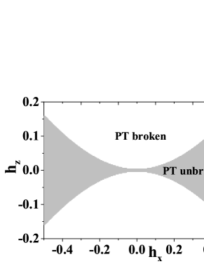
Figure 7: (Color online) The phase diagram of $\mathcal{PT}$-symmetry spontaneous breaking for the topologically degenerate ground states on $2\ast 3$ lattice. The phase boundary is exceptional points.

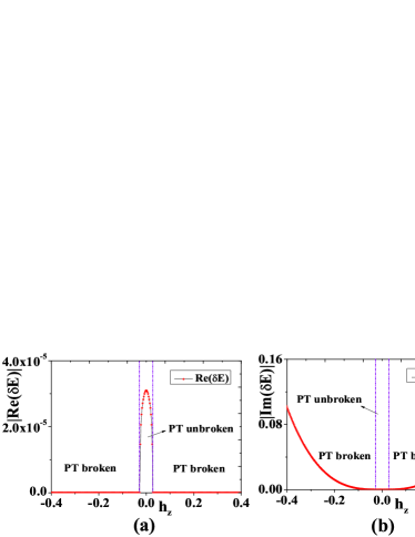
Figure 8: (Color online) (a)(b) The absolute value of real part and imaginary of energy splitting for the two degenerate ground states for the case of $h_{x}=0.2$ via $h_{z}$ based on the non-Hermitian Wen-plaquette model on $2\ast 3$ lattice.

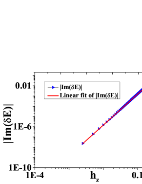
Figure 9: (Color online) The absolute value of imaginary parts of energy splitting between the two degenerate ground states $\left|\operatorname{Im}(\delta E)\right|$ for the case of $h_{x}=0$ via $h_{z}$ on $2\ast 3$ lattice.

In Fig.7, Fig.8 and Fig.9, we plot the numerical results from the exact diagonalization technique of the non-Hermitian Wen-plaquette model $\hat{H}_{\mathrm{NTO}}$ on $2\ast 3$ lattice with periodic boundary conditions. Fig.7 shows the global phase diagram of $\mathcal{PT}$-symmetry-breaking transition for topologically degenerate ground states. The phase boundary are all exceptional points characterized by the relation $\alpha(h_{x})^{6}=\beta(h_{z})^{3}$. In Fig.8(a) and Fig.8(b), we plot the absolute value of real part ($\left|\operatorname{Re}(\delta E)\right|$) and imaginary ($\left|\operatorname{Im}(\delta E)\right|$) of energy splitting for the two degenerate ground states for the non-Hermitian Wen-plaquette model $\hat{H}_{\mathrm{NTO}}$ with $h_{x}=0.2$ on $2\ast 3$ lattice, respectively. The results ($\left|\operatorname{Im}(\delta E)\right|$) in Fig.9 are consistent to theoretical prediction: the step of dynamic strings for fermions is $3.01$ from the numerical results (the theoretical prediction is $3$).

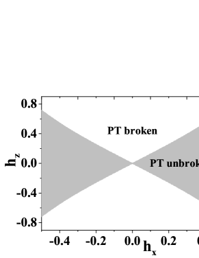
Figure 10: (Color online) The phase diagram of $\mathcal{PT}$-symmetry spontaneous breaking for the topologically degenerate ground states on $3\ast 3$ lattice. The phase boundary is exceptional points.

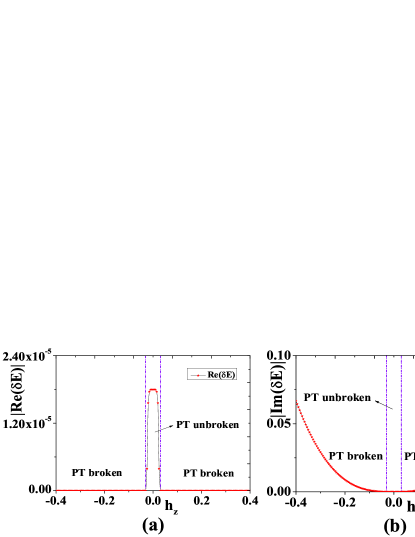
Figure 11: (Color online) (a)(b) The absolute value of real part and imaginary of energy splitting for the two degenerate ground states for the case of $h_{x}=0.02$ via $h_{z}$ based on the non-Hermitian Wen-plaquette model on $3\ast 3$ lattice.

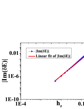
Figure 12: (Color online) The absolute value of imaginary parts of energy splitting between the two degenerate ground states $\left|\operatorname{Im}(\delta E)\right|$ for the case of $h_{x}=0$ via $h_{z}$ on $3\ast 3$ lattice.

In Fig.10, Fig.11 and Fig.12, we plot the numerical results from the exact diagonalization technique of the non-Hermitian Wen-plaquette model $\hat{H}_{\mathrm{NTO}}$ on $3\ast 3$ lattice with periodic boundary conditions. Fig.10 shows the global phase diagram of $\mathcal{PT}$-symmetry-breaking transition for topologically degenerate ground states. The phase boundary are exceptional points characterized by the relation $h_{z}\sim h_{x}$, which is agreement with the result from pseudo-spin model above $\alpha h_{x}^{3}=\beta(h_{z})^{3}$. In Fig.11(a) and Fig.11(b), we plot the absolute value of real parts and imaginary parts of energy splitting for the two topologically degenerate ground states for the non-Hermitian Wen-plaquette model with $h_{x}=0.02$ on $3\ast 3$ lattice, respectively. In Fig.12, the absolute value of imaginary parts of energy splitting between the two degenerate ground states of the non-Hermitian Wen-plaquette (toric-code) model is obtained with $h_{x}=0$ on $3\ast 3$ lattice. The numerical result indicates that the step of dynamic strings for fermions is $2.92$, which is consistent with theoretical prediction $3$.

VI.4 Application

It was pointed out that the topological degenerate ground states for a $Z_{2}$ topological order make up a protected subspace free from errork1 ; k2 ; kou1 ; kou2 ; kou3 . One can manipulate the protected subspace by controlling their quantum tunneling effectkou1 ; kou2 ; kou3 ; md1 . However, due to the very tiny value of energy splitting for topological degenerate ground states, the initialization topological degenerate ground states for quantum computation based on such topological qubits becomes very difficult. As a result, we propose a new approach to initialize the system (for example, the topological degenerate ground states on an $e\ast o$ lattice) into a particular state. The basic idea is to drive the topological qubit to exceptional points by adding (real or imaginary) external field and then removal it slowly.

The evolution will occur along the exceptional points according to the Hamiltonian

$$\hat{H}_{\mathrm{NTO}}(t)=\hat{H}_{\mathrm{TO}}+{\displaystyle\sum\limits_{i}}[h_{x}(t)\sigma_{i}^{x}+ih_{z}(t)\sigma_{i}^{z}],$$ (93)

where

$$h_{x}{(t)={h}_{0}(1-e}^{t/t_{0}}),$$ (94)

and

$$h_{z}(t)=(\frac{\alpha}{\beta})^{\frac{1}{L_{y}}}(h_{x}(t))^{\frac{L_{x}}{\xi}}.$$ (95)

At the beginning, $t\rightarrow-\infty,$ under the finite external field ${h}_{x}{(t),}$ ${h_{z}(t),}$ the system is at exceptional points. The effective Hamiltonian of the topological qubit in the external field

$$\mathcal{\hat{H}}_{\mathrm{eff}}^{e\ast o}(t)=\frac{\Delta(t)}{2}(\tau^{x}+i\tau^{z}).$$ (96)

Due to the non-Hermitian term, the topological degeneracy is reduced into non-Hermitian degeneracy at the exceptional points. As a result, there doesn’t exist topological degeneracy and the two topological degenerate ground states merge into one quantum ”steady” state,

$$\left|\psi_{+}\right\rangle\rightarrow\left|\uparrow\right\rangle_{R}-i\left|\downarrow\right\rangle_{R}\Leftrightarrow\left|\psi_{-}\right\rangle\rightarrow\left|\uparrow\right\rangle_{R}-i\left|\downarrow\right\rangle_{R}.$$ (97)

At the time $t=0,$ when the external field disappears, ${h_{x}(t),}$ ${h_{z}(t)=0}$, a pure quantum state for quantum computation based on topological qubits is initialized as

$$\left|\uparrow\right\rangle_{R}-i\left|\downarrow\right\rangle_{R}.$$ (98)

This approach to initialization for topological qubits is much more efficiency than the traditional approach by adding a (pure) real external field in Ref.kou1 ; kou2 ; kou3 .

VII Conclusion

In this paper, we developed a theory of the non-Hermitian $Z_{2}$ topological order. The quantum states of non-Hermitian $Z_{2}$ topological order are characterized by different Hermitian/non-Hermitian dynamic strings. The ground states of non-Hermitian Wen-plaquette model on a torus are classified by different Hermitian/non-Hermitian topological closed dynamic strings. The effective model for the topologically degenerate ground states on $e\ast o$, or $o\ast e,$ or $o\ast o$ lattices can be mapped onto an effective non-Hermitian pseudo-spin model, from which the anomalous topological degeneracy occurs. In particular, there exists spontaneous $\mathcal{PT}$ symmetry breaking for the topologically degenerate ground states. At “exceptional points”, the topologically degenerate ground states merge and the topological degeneracy turns into non-Hermitian degeneracy. In the end, the application of the non-Hermitian $Z_{2}$ topological order and its possible physics realization are discussed. In addition, this work may help people to understanding the effect of non-Hermitian perturbations on many-body systems.

In the end, we address the experimental realization of the non-Hermitian $Z_{2}$ topological order. It is still of challenge both to experimentally investigate $\mathcal{PT}$ symmetric Hamiltonian related physics in quantum systems and to realize the toric-code model. A possible approach is cold-atom experiments: On the one hand, non-Hermitian Hamiltonians arise in cold-atom experiments due to spontaneous decayHang2013 ; Lee2014 ; luo ; On the other hand, a small system for toric-code model with open boundary condition has also been realized in cold atomsyuan .

- (1) C. M. Bender, and S. Boettcher, Phys. Rev. Lett. 80, 5243 (1998).C. M. Bender, D. C. Brody, and H. F. Jones, Phys. Rev. Lett. 89, 270401 (2002).C. M. Bender, Rep. Prog. Phys. 70, 947 (2007).
- (2) A. Guo, G. J. Salamo, D. Duchesne, R. Morandotti, M. Volatier-Ravat, V. Aimez, G. A. Siviloglou, and D. N. Christodoulides, Phys. Rev. Lett. 103, 093902 (2009).
- (3) C. E. Rüter, K. G. Makris, R.El-Ganainy, D. N. Christodoulides, M. Segev, and D. Kip, Nat. Phys. 6, 192 (2010).
- (4) Y. D. Chong, L. Ge, and A. D. Stone, , Phys. Rev. Lett. 106, 093902 (2011)
- (5) A. Regensburger, C. Bersch, M.-A. Miri, G. Onishchukov, D. N. Christodoulides, and U. Peschel, Nature (London) 488, 167 (2012).
- (6) L. Feng, Y.-L. Xu, W. S. Fegadolli, M.-H. Lu, J. E. B. Oliveira, V. R. Almeida, Y.-F. Chen, and A. Scherer, Nat. Mater. 12, 108 (2013).
- (7) M. Wimmer, M. A. Miri, D. N. Christodoulides, and U. Peschel, Sci. Rep. 5, 17760 (2015).
- (8) S. Weimann, M. Kremer, Y. Plotnik, Y. Lumer, S. Nolte, K. G. Makris, M. Segev, M. C. Rechtsman, and A. Szameit, Nat. Mater. 16, 433 (2017).
- (9) H. Hodaei, A. U. Hassan, S. Wittek, H. Garcia-Gracia, R. El-Ganainy, D. N. Christodoulides, and M. Khajavikhan, Nature (London) 548, 187 (2017).
- (10) Ş. K. Özdemir, S. Rotter, F. Nori, and L Yang, Nat. Mater. 18, 783 (2019).
- (11) J. Schindler, A. Li, M. C. Zheng, F. M. Ellis, and T. Kottos, Phys. Rev. A 84, 040101 (2011)
- (12) S. Assawaworrarit, X. Yu, and S. Fan, Nature 546, 387 (2017).
- (13) Y. Choi, C. Hahn, J. W. Yoon, and S. H. Song, Nat. Commun. 9, 2182 (2018).
- (14) S. Bittner, B. Dietz, U. Günther, H. L. Harney, M. Miski-Oglu, A. Richter, and F. Schäfer, Phys. Rev. Lett. 108, 024101 (2012).
- (15) B. Peng, Ş. K. Özdemir, F. Lei, F. Monifi, M. Gianfreda, G. L. Long, S. Fan, F. Nori, C. M. Bender, and L. Yang, Nat. Phys. 10, 394 (2014).
- (16) C. Poli, M. Bellec, U. Kuhl, F. Mortessagne, and H. Schomerus, Nat. Commun. 6, 6710 (2015).
- (17) Z.-P. Liu, J. Zhang, Ş. K. Özdemir, B. Peng, H. Jing, X.-Y. Lü, C.-W. Li, L. Yang, F. Nori, and Y.-X. Liu,, Phys. Rev. Lett. 117, 110802 (2016).
- (18) X. Zhu, H. Ramezani, C. Shi, J. Zhu, and X. Zhang, Phys. Rev. X 4, 031042 (2014).
- (19) B. I. Popa, and S. A. Cummer, Nat. Commun. 5, 3398 (2014).
- (20) R. Fleury, D. Sounas, and A. Alu, Nat. Commun. 6, 5905 (2015).
- (21) K. Ding, G. Ma, M. Xiao, Z. Q. Zhang, and C. T. Chan, Phys. Rev. X 6, 021007 (2016)
- (22) Y. Wu, W. Liu, J. Geng, X. Song, X. Ye, C. K. Duan, X. Rong and J. Du, Science, 364, 878(2019).
- (23) L. Xiao, X. Zhan, Z. H. Bian, K. K. Wang, X. Zhang, X. P. Wang, J. Li, K. Mochizuki, D. Kim, N. Kawakami, W. Yi, H. Obuse, B. C. Sanders, and P. Xue, Nat. Phys. 13, 1117 (2017).
- (24) J. Li, A. K. Harter, J. Liu, L. de Melo, Y. N. Joglekar, and L. Luo, Nat. Commun. 10, 855 (2019).
- (25) L. Xiao, K. Wang, X. Zhan, Z. Bian, K. Kawabata, M. Ueda, W. Yi, and P. Xue, Phys. Rev. Lett. 123, 230401 (2019).
- (26) K. Wang, X. Qiu, L. Xiao, X. Zhan, Z. Bian, B. C. Sanders, W. Yi, and P. Xue, Nat. Commun. 10, 2293 (2019).
- (27) L. Feng, Z. J. Wong, R. M. Ma, Y. Wang, and X. Zhang, Science, 346 972 (2014).
- (28) H. Hodaei, M. A. Miri, M. Heinrich, D. N. Christodoulides, and M. Khajavikhan, Science, 346, 975 (2014).
- (29) M. S. Rudner and L. S. Levitov, Phys. Rev. Lett. 102, 065703 (2009).
- (30) K. Esaki, M. Sato, K. Hasebe, and M. Kohmoto, Phys. Rev. B 84, 205128 (2011).
- (31) Y. C. Hu and T. L. Hughes, Phys. Rev. B 84, 153101 (2011).
- (32) S.-D. Liang and G.-Y. Huang, Phys. Rev. A 87, 012118 (2013).
- (33) B. Zhu, R. Lü, and S. Chen, Phys. Rev. A 89, 062102 (2014).
- (34) T. E. Lee, Phys. Rev. Lett. 116, 133903 (2016).
- (35) P. San-Jose, J. Cayao, E. Prada, and R. Aguado, Sci. Rep. 6, 21427 (2016).
- (36) D. Leykam, K. Y. Bliokh, C. Huang, Y. D. Chong, and F. Nori, Phys. Rev. Lett. 118, 040401 (2017).
- (37) H. Shen, B. Zhen, and L. Fu, Phys. Rev. Lett. 120, 146402 (2018).
- (38) S. Lieu, Phys. Rev. B 97, 045106 (2018).
- (39) Y. Xiong, J. Phys. Commun. 2, 035043 (2018).
- (40) K. Kawabata, Y. Ashida, H. Katsura, and M. Ueda, Phys. Rev. B 98, 085116 (2018).
- (41) Z. Gong, Y. Ashida, K. Kawabata, K. Takasan, S. Higashikawa, and M. Ueda, Phys. Rev. X 8, 031079 (2018).
- (42) S. Yao, and Z. Wang, Phys. Rev. Lett. 121, 086803 (2018).
- (43) S. Yao, F. Song, and Z. Wang, Phys. Rev. Lett. 121, 136802 (2018).
- (44) F. K. Kunst, E. Edvardsson, J. C. Budich, and E. J. Bergholtz, Phys. Rev. Lett. 121, 026808 (2018).
- (45) C. Yin, H. Jiang, L. Li, R. Lü, and S. Chen, Phys. Rev. A 97, 052115 (2018).
- (46) K. Kawabata, K. Shiozaki, and M. Ueda, Phys. Rev. B 98, 165148 (2018).
- (47) V. M. M. Alvarez, J. E. B. Vargas, M. Berdakin, and L. E. F. F. Torres, Eur. Phys. J. Spec. Top. 227, 1295 (2018).
- (48) H. Jiang, C. Yang, and S. Chen, Phys. Rev. A 98, 052116 (2018).
- (49) A. Ghatak and T. Das, J. Phys.: Condens. Matter 31, 263001 (2019).
- (50) J. Avila, F. Peñranda, E. Prada, P. San-Jose, and R. Aguado, Commun. Phys. 2, 1 (2019).
- (51) L. Jin and Z. Song, Phys. Rev. B 99, 081103 (2019); S. Lin, L. Jin, and Z. Song, Phys. Rev. B 99, 165148 (2019); K. L. Zhang, H. C. Wu, L. Jin, and Z. Song, Phys. Rev. B 100, 045141 (2019).
- (52) C. H. Lee and R. Thomale, Phys. Rev. B 99, 201103(R) (2019).
- (53) T. Liu, Y.-R. Zhang, Q. Ai, Z. Gong, K. Kawabata, M. Ueda, and F. Nori, Phys. Rev. Lett. 122, 076801 (2019).
- (54) K. Kawabata, K. Shiozaki, M. Ueda, and M. Sato, Phys. Rev. X 9, 041015 (2019).
- (55) H. Zhou and J. Y. Lee, Phys. Rev. B 99, 235112 (2019).
- (56) C. H. Liu, H. Jiang, S. Chen, Phys. Rev. B 99, 125103 (2019).
- (57) E. Edvardsson, F. K. Kunst, and E. J. Bergholtz, Phys. Rev. B 99, 081302(R) (2019).
- (58) L. Herviou, J. H. Bardarson, and N. Regnault, Phys. Rev. A 99, 052118 (2019).
- (59) K. Yokomizo and S. Murakami, Phys. Rev. Lett. 123, 066404 (2019).
- (60) F. K. Kunst and V. Dwivedi, Phys. Rev. B 99, 245116 (2019).
- (61) R. Chen, C.-Z. Chen, B. Zhou, and D.-H. Xu, Phys. Rev. B 99, 155431 (2019).
- (62) T. S. Deng and W. Yi, Phys. Rev. B 100, 035102 (2019).
- (63) F. Song, S. Yao, and Z. Wang, Phys. Rev. L 123, 170401 (2019).
- (64) Xi-Wang Luo and Chuanwei Zhang, Phys. Rev. Lett. 123 073601 (2019).
- (65) S. Longhi, Phys. Rev. Research 1, 023013 (2019).
- (66) H Jiang, R Lü, S Chen, arXiv:1906.04700.
- (67) X.-G. Wen, Quantum Field Theory of Many-Body Systems, (Oxford Univ. Press, Oxford, 2004).
- (68) A. Kitaev, Annals Phys. 303, 2 (2003).
- (69) A. Kitaev, Annals Phys. 321, 2 (2006).
- (70) X. G. Wen, Phys. Rev. Lett. 90, 016803 (2003).
- (71) X. G. Wen, Phys. Rev. D 68, 065003 (2003).
- (72) S. P. Kou, Phys. Rev. Lett. 102, 120402 (2009).
- (73) J. Yu and S. P. Kou, Phys. Rev. B 80, 075107 (2009).
- (74) S. P. Kou, Phys. Rev. A 80, 052317 (2009).
- (75) H. Bombin, M.A. Martin-Delgado, Phys. Rev. Lett. 97, 180501 (2006); D. Vodola, D. Amaro, M. A. Martin-Delgado, and M. Müller, Phys. Rev. Lett. 121, 060501 (2018).
- (76) A. Mostafazadeh, J. Math. Phys 43, (2002) 205, 2824, 3944; ibid 44, (2003) 974.
- (77) H. Ramezani, T. Kottos, R. El-Ganainy, and D. N. Christodoulides, Phys. Rev. A 82, 043803 (2010).
- (78) D. Nigg, M. Muller, E. A. Martinez, P. Schindler, M. Hennrich, T. Monz, M. A. Martin-Delgado, R. Blatt. Science 345. 302 (2014).
- (79) C. Hang, G. Huang, and V. V. Konotop, Phys. Rev. Lett. 110, 083604 (2013).
- (80) T. E. Lee and C.-K. Chan, Phys. Rev. X 4, 041001 (2014).
- (81) H. N. Dai, B. Yang, A. Reingruber, H. Sun, X. F. Xu, Y. A. Chen, Z. S. Yuan and J. W. Pan, Nat. Phys. 13, 1195 (2017).