Measuring neutrino masses with large-scale structure: Euclid forecast with controlled theoretical error

Abstract

We present a Markov-Chain Monte-Carlo (MCMC) forecast for the precision of neutrino mass and cosmological parameter measurements with a Euclid-like galaxy clustering survey. We use a complete perturbation theory model for the galaxy one-loop power spectrum and tree-level bispectrum, which includes bias, redshift space distortions, IR resummation for baryon acoustic oscillations and UV counterterms. The latter encapsulate various effects of short-scale dynamics which cannot be modeled within perturbation theory. Our MCMC procedure consistently computes the non-linear power spectra and bispectra as we scan over different cosmologies. The second ingredient of our approach is the theoretical error covariance which captures uncertainties due to higher-order non-linear corrections omitted in our model. Having specified characteristics of a Euclid-like spectroscopic survey, we generate and fit mock galaxy power spectrum and bispectrum likelihoods. Our results suggest that even under very agnostic assumptions about non-linearities and short-scale physics a future Euclid-like survey will be able to measure the sum of neutrino masses with a standard deviation of 28 meV. When combined with the Planck cosmic microwave background likelihood, this uncertainty decreases to 13 meV. Over-optimistically reducing the theoretical error on the bispectrum down to the two-loop level marginally tightens this bound to 11 meV. Moreover, we show that the future large-scale structure (LSS) spectroscopic data will greatly improve constraints on the other cosmological parameters, e.g. reaching a percent (per mille) error on the Hubble constant with LSS alone (LSS + Planck).

INR-TH-2019-014

1 Introduction

The detection of neutrino flavor oscillations has revealed that neutrinos have at least three individual mass states. The neutrino masses are described by the dimension-5 Weinberg operator in the Standard model treated as an effective field theory. Thus, the neutrino mass scale hints on the energy cutoff above which the Standard model must be completed, and constrains its possible extensions. The target value relevant for particle physics model building is $100$ meV, which would allow one to discriminate between two different hierarchies: normal (two light states and one more massive one) or inverted (one light state and two massive ones) [1, 2].

Laboratory oscillation experiments are only sensitive to the mass gap between various neutrino species and bound the total neutrino mass $\sum m_{\nu}$ to be above $60$ meV. An upper limit can be obtained by measuring the edge of the electron spectrum in $\rm{}^{3}H$ $\beta$-decay experiments [3, 4, 5, 6]. Using this method, the ‘Troitsk nu-mass’ experiment obtained the bound on the neutrino mass for the electron antineutrino $\bar{\nu}_{e}$, $m_{\bar{\nu}_{e}}<2.05\,\text{eV}\,(2\sigma)$ [3, 6]. In principle, the sensitivity to $m_{\bar{\nu}_{e}}$ can be improved down to $\sim 0.2\,\text{eV}$ with the ongoing KATRIN facility [5], which recently obtained the most stringent laboratory bound to date $\sum m_{\nu}<1.1\,\text{eV}\,(90\%\text{CL}.)$ [7]. However, further progress toward a more accurate measurement of the absolute neutrino mass may be challenging with current technologies.

As of now, the most stringent upper bound on the total neutrino mass comes from cosmology. The Planck cosmic microwave background (CMB) observations have set a $2\sigma$ upper limit $240$ meV from the CMB data alone [8]. Combining CMB with measurements of the scale of baryon acoustic oscillations (BAO) tightens this constraint down to $120$ meV. Similar bounds have been obtained by combining the CMB data with the Ly$\alpha$-flux measurements [9], the Sunyaev-Zeldovich power spectrum and cluster counts [10], and the full-shape galaxy clustering measurements, e.g. [11, 12, 13, 14, 15, 16]. In general, the combination of large-scale structure (LSS) and CMB data is essential for the neutrino mass measurements [17, 18, 19, 20, 21, 22]. However, in principle, some constraints can be derived from the LSS data alone, even though currently the LSS data per se are not competitive with the CMB measurements [23].

The situation will likely change in the near future as we enter the era of high precision LSS data. Next-generation surveys (e.g. SKA, LSST, DESI, Euclid) will map a large volume of the Universe and generate a highly detailed three-dimensional galaxy distribution. For example, the Euclid satellite is expected to measure more than 50 million redshifts of distant galaxies over a large fraction of the sky [24] and thus harvest a huge amount of information about galaxy clustering at different scales and redshifts. This offers a unique opportunity to improve measurements of cosmological parameters including the total neutrino mass. However, the LSS data analysis is complicated by effects of non-linear clustering, galaxy bias and redshift space distortions. Our ability to fully exploit the potential of upcoming surveys will strongly depend on the understanding on these effects, which is not yet complete.

Fortunately, the bulk of information about the neutrino free-streaming is encoded in mildly non-linear scales which can be robustly and systematically described within perturbation theory. One of the most popular approaches is Eulerian standard cosmological perturbation theory (SPT) [25]. The basic formulation of SPT, however, does not correctly capture the non-linear evolution of baryon acoustic oscillations (BAO) [26] and short-scale physics beyond the single-stream pressureless perfect fluid hydrodynamics [27, 28, 29]. These problems have been intensely studied in the recent years.

First, it has been shown that the non-linear suppression and distortion of the BAO can be captured by a resummation of contributions describing the tidal effects of large-scale bulk flows. This procedure, called infrared (IR) resummation, is essential for an accurate description of the BAO and has been formulated within various theoretical frameworks [30, 31, 32, 33, 34, 35]. We will adopt a systematic approach of [32, 34] streamlined in the context of time-sliced perturbation theory [36].

Second, we will use the effective field theory of large-scale structure (EFT) to account for the back-reaction of small scale nonlinearities on larger scales [28, 37, 38]. This approach removes the unphysical UV sensitivity of perturbation theory loop integrals and parameterizes the ignorance about short scale-dynamics by various effective operators in the equations of motion for the dark matter fluid. The EFT addresses rather general short-scale phenomena including halo virialization, baryonic feedback, and the fingers-of-God effect due to virialized motions. These phenomena are encapsulated in a number of free parameters, called “counterterms,” whose values and time-dependences are not known a priori.

Third, we will employ the full non-linear bias model. Galaxies are biased tracers of the underlying matter field which consists of baryons and dark matter. The relation between matter and galaxies on large scales is encapsulated in a perturbative expansion built out of all possible operators allowed by rotational symmetry and the equivalence principle [39, 40, 41, 42]. The relevance of these operators is controlled by the corresponding non-linear bias coefficients. One could try to derive bias parameters analytically or extract them from N-body simulations [43, 44, 45, 46]. In this work we adopt an agnostic approach for the bias expansion. We will treat both the counterterms and bias coefficients as nuisance parameters and marginalize over their values and time-dependence.

The galaxy distribution is commonly characterized by the two-point correlation function or its Fourier space counterpart, power spectrum. The power spectrum analysis, however, suffers from degeneracies between cosmological and bias parameters. This problem can be alleviated by adding the information from the tree-point correlation function, or its Fourier space counterpart called “bispectrum.” The bispectrum introduces new shape dependencies that break parameter degeneracies and yield more robust constraints on cosmological parameters [47, 48, 49, 50, 51, 52].

It is desirable to use the Markov Chain Monte Carlo (MCMC) technique for parameter inference from LSS surveys. This is a common practice for the CMB, weak lensing and photometric galaxy clustering data, but not in the full-shape (FS) Fourier-space power spectrum analysis [53]. The main goal of the recent FS analyses is the measurement of the radial and angular diameter distances from the Alcock-Paczynski (AP) effect [55], and the amplitude of velocity fluctuations $f\sigma_{8}$ probed by redshift-space distortions. In that case one usually keeps the shape of the power spectrum fixed, which is correct if one does not vary the physical densities of massive neutrinos, dark matter and baryons, $\Omega_{\nu}h^{2}$, $\Omega_{cdm}h^{2}$ and $\Omega_{b}h^{2}$, respectively. The latter two have been measured by the CMB data significantly more precisely than by any other observation. This justifies the standard practice for the baseline BOSS power spectrum model with the minimal neutrino mass. This practice clearly becomes inaccurate if one varies the neutrino masses, which generates peculiar scale-dependent shape distortions of the power spectrum. Besides, the precision of the upcoming LSS surveys can surpass the CMB precision, in which case the standard approach will also be inadequate. In these situations it is imperative to vary all cosmological parameters in MCMC chains and consistently recompute the shape of the non-linear power spectrum during the sampling.

Performing a full MCMC analysis for the Fourier space power spectrum was unfeasible for a long time because the calculation of perturbation theory convolution integrals was not fast enough. Recently, there have been a number of attempts to boost the computational efficiency by using some advanced numerical algorithms [56, 57, 58, 59]. In our work we will employ the FFTLog method originally proposed in Ref. [60] and recently revisited in the context of perturbation theory loop integrals in [59]. In this approach the linear matter power spectrum is decomposed over a basis of power-law functions, whose convolution integrals can be done analytically. We implement this algorithm in the publicly available CLASS code [61] and show that its performance is fast enough for MCMC parameter estimation. To our knowledge, the present analysis is the first MCMC forecast of an LSS survey that features a consistent perturbative treatment of non-linearities and other short-scale phenomena for galaxies in redshift space.

Another important ingredient of our study is the theoretical error covariance. Perturbative calculations of a given order are valid only for a limited range of scales where the next-order corrections are small. These corrections can be estimated and added to the covariance matrix as a correlated error. This approach was pioneered in Ref. [19] and was recently revisited in the context of perturbation theory in Ref. [62]. The theoretical error method is different from a usually employed approach of trusting the theory completely until a certain wavenumber $k_{\text{max}}$ [49, 21, 63, 64]. Using such a cut-off means that all information coming from wavenumbers higher than $k_{\text{max}}$ is thrown away. However, the theoretical error grows gradually as a function of the wavenumber and is correlated across different $k$-bins. This implies that even the short scales dominated by the theoretical error can still yield some cosmological information. For example, the BAO wiggles in the matter power spectrum can be accurately described even at the scales where the broadband part can have a large theoretical uncertainty, see e.g. Ref. [65] for a related study. If the coherence frequency of this uncertainty is bigger than the BAO frequency, the BAO wiggles will still have a significant signal-to-noise even if they are superimposed on top of a poorly known broadband signal. The situation here is similar to the common BAO scale measurements upon marginalizing over the broadband shape [66].

Our paper has several objectives. First, we demonstrate that cosmological parameters can be extracted from a spectroscopic galaxy survey by means of an MCMC analysis of the full shape power spectrum and bispectrum data. This includes a rigorous computation of non-linear loop corrections for each sampled set of cosmological parameters. Second, we show that even under the most agnostic assumptions about the short-scale physics and galaxy bias one is still able to obtain decent constraints on the total neutrino mass and cosmological parameters of the minimal $\Lambda$CDM. Third, we scrutinize various effects forming the neutrino mass constraints: redshift space distortions, the Alcock-Paczynski effect, baryon acoustic oscillations, inclusion of the bispectrum, and combination of LSS measurements with the CMB data.

The sensitivity of upcoming LSS surveys to neutrino masses has been studied in a number of works [67, 19, 62, 68, 69, 63, 22, 70, 64, 71, 72, 73]. In this paper we combine, for the first time, all important ingredients of the analysis. First, we use a full MCMC approach which accurately captures relevant parameter correlations and is free from inaccuracies of the Fisher matrix calculus. Second, we use a complete one-loop perturbation theory model for the redshift-space galaxy power spectrum, and adopt a conservative approach to nuisance parameters describing non-linear short-scale dynamics, baryonic effects, bias and redshift space distortions. Third, we add the tree-level bispectrum likelihood to the analysis. Our baseline theoretical model includes the one-loop power spectrum with all relevant nuisance parameters, and the tree-level bispectrum, which includes quadratic bias parameters. Thus, we consistently take into account all perturbative corrections up to the third order in the linear density field. Fourth, we employ the theoretical error covariance, which is based on perturbation theory arguments and does not require any input from N-body simulations.

The paper is organized as follows. Section 2 discusses our theoretical model. Section 3 specifies the Euclid galaxy survey and fixes fiducial parameters for our mock datasets. In Section 4 we give a detailed description of our method and the covariance matrix treatment, including the theoretical error. The readers who are not interested in the technical aspects of our analysis can jump directly to Section 5, where we present results of our MCMC parameter extraction and discuss how various effects contribute to the constraints on the neutrino masses and cosmological parameters. We conclude in Section 6. Some supplementary material is collected in the Appendices. We give explicit expressions for the one-loop redshift space galaxy power spectrum in Appendix A and the corresponding covariance matrix in Appendix B. Appendix C scrutinizes the information content of the BAO wiggles. Appendix D presents results for the worst-case scenario of the theoretical error with a strong fingers-of-God effect. Appendix E shows that using a sharp momentum cutoff or the linear power spectrum model can significantly degrade the forecasted constraints. Finally, Appendix F contains the results obtained by using the Planck Gaussian prior on the cosmological parameters instead of the full likelihood.

2 Theoretical Model

We will use cosmological perturbation theory to compute templates for the galaxy power spectrum and bispectrum. Let us briefly discuss some general approximations which we will make. These approximation are common in the LSS literature. Our theoretical model will be an extension of standard Eulerian perturbation theory [25], which is based on several core assumptions. First, SPT assumes that the dynamics of matter on large scales is governed by the Eulerian pressureless perfect fluid hydrodynamics. Second, SPT assumes that the initial density field is a Gaussian stochastic variable and its rms deviations are small on large scales. Third, SPT uses the so-called Einstein de-Sitter (EdS) approximation, i.e. the time-dependence of loop corrections is factored out and approximated by powers of the linear growth factor just like in a matter-dominated (Einstein de-Sitter) universe. This approximation was checked to be sub-percent accurate on mildly non-linear scales [76, 77]. In this paper we will go beyond the first approximation and take into account corrections to the pressureless perfect fluid dynamics within effective field theory (EFT). As we argue now, the latter two SPT assumptions mentioned above need not be revisited for the purposes of our study.

The presence of massive neutrinos requires several modifications to the standard formalism. Most importantly, the linear growth rate of matter fluctuations becomes wavenumber-dependent. This happens because matter clustering slows down on scales smaller than the free-streaming length after the neutrinos become non-relativistic. Strictly speaking, the EdS factorization does not take place in this case. A proper perturbative treatment requires an accurate calculation of the scale-dependent Green’s function [78, 79, 80]. This approach is quite laborious and has not yet been extended to galaxies in redshift space. To overcome this difficulty we adopt the following approximation. For a given redshift we will evaluate non-linear predictions with the standard perturbation theory kernels, but using the exact linear matter power spectrum computed in the presence of massive neutrinos [81]. This approximation was shown to agree with the full calculation within a two-fluid extension of standard perturbation theory with a few percent precision [78]. Recently, this result was confirmed within the EFT [80], which showed that the residual difference between the full calculation and the EdS can be absorbed into the $k^{2}$-counterterm (to be discussed shortly). This suggests that the EdS approximation with the appropriate countertems will be sufficient for the precision of upcoming LSS surveys. We emphasize that the EdS approximation takes into account the leading non-trivial time- and scale-dependence of the perturbation theory Green’s functions in the presence of massive neutrinos.

As far as the bispectrum is concerned, recent analytic and numerical analyses [82, 83] have shown that on mildly non-linear scales the neutrino effect is also dominated by the free-streaming damping of the linear matter power spectrum. In other words, the power spectrum picture presented above applies to the bispectrum as well.

To sum up, for the purposes of this paper the leading effect of massive neutrinos on matter clustering can be approximated as a time- and scale-dependent suppression of the linear density field. All more complicated phenomenology beyond this approximation, e.g. [84, 85, 79, 86, 87, 88] is captured by the EFT corrections (counterterms) [80]. Now let us discuss in detail various ingredients of our theoretical approach.

2.1 Non-linear galaxy bias

Galaxies are biased tracers of the underlying matter density field. Galaxy bias has been a subject of various studies carried out over last years, e.g. see [39, 40, 41] and [42] for a comprehensive review. In our base bias model we assume that the clustering properties of galaxies are determined by the dark matter and baryons, and not by the total matter including massive neutrinos. This approach, called the “cb” prescription, has a simple physical interpretation: halos form on short scales where the neutrinos have significant velocity dispersion and hence do not participate in clustering. The “cb” prescription was first advocated on the basis of N-body simulations [89, 90, 91, 92] and then explained theoretically in Ref. [93]. Moreover, Refs. [69, 70] pointed out its importance for parameter inference. Note that within our prescription all the matter statistics, e.g. the linear power spectrum $P_{\text{lin}}(k)$ will refer to cold dark matter and baryons without massive neutrinos.

In perturbation theory the galaxy density contrast $\delta_{g}$ is generally expressed as a series of operators that are constructed out of the Newtonian gravitational potential $\Phi$ and the velocity potential $\Phi_{v}$, and satisfy rotational symmetry and the equivalence principle. For the purposes of this paper the bias expansion will be built upon the cold dark matter + baryon (cb) density fields $\delta_{\text{cb}}$, hence $\Phi$ and $\Phi_{v}$ will refer to the effective potentials sourced by the ‘cb’ fluid. The expansion sufficient for the one-loop matter power spectrum is

$$\begin{split}\delta_{g}=&\leavevmode\nobreak\ b_{1}\delta_{\text{cb}}+\varepsilon-R^{2}_{*}k^{2}\delta_{\text{cb}}+\frac{\displaystyle b_{2}}{\displaystyle 2}\delta^{2}_{\text{cb}}+b_{\mathcal{G}_{2}}\mathcal{G}_{2}\\ &\leavevmode\nobreak\ +\frac{b_{3}}{6}\delta^{3}_{\text{cb}}+b_{\mathcal{G}_{3}}\mathcal{G}_{3}+b_{(\mathcal{G}_{2}\delta)}\mathcal{G}_{2}\delta_{\text{cb}}+b_{\Gamma_{3}}\Gamma_{3}\,,\end{split}$$ (2.1)

where $\varepsilon$ is the stochastic part which is not correlated with the large-scale density field, and we introduced the following operators:

$${}\begin{split}{}&\mathcal{G}_{2}(\Phi)\equiv(\partial_{i}\partial_{j}\Phi)^{2}-(\partial^{2}\Phi)^{2}\,,\\ &\mathcal{G}_{3}(\Phi)\equiv-\partial_{i}\partial_{j}\Phi\partial_{j}\partial_{k}\Phi\partial_{k}\partial_{i}\Phi-\frac{1}{2}(\partial^{2}\Phi)^{3}+\frac{3}{2}(\partial_{i}\partial_{j}\Phi)^{2}\partial^{2}\Phi\,,\\ &\Gamma_{3}\equiv\mathcal{G}_{2}(\Phi)-\mathcal{G}_{2}(\Phi_{v})\,.\end{split}$$ (2.2)

The $k^{2}R_{*}^{2}\delta_{\text{cb}}$ contribution in (2.1) is the so-called higher-derivative bias, which is characterized by a length scale $R_{*}$. For the higher derivative expansion to make sense one demands that $R^{2}_{*}k^{2}\ll 1$. Higher-derivative terms are expected to originate from an effective viscous tensor in the Euler equation, which accounts for the effects of shell-crossing and virialization. On dimensional grounds one may expect that $R_{*}$ should be given by the Lagrangian radius of typical halos that host the galaxies of interest. However, the higher-derivative operator also encapsulates other effects of short-scale dynamics beyond the pressureless perfect-fluid approximation. First, it corrects for the error introduced by integrating over infinite momenta in standard perturbation theory loop integrals. Indeed, the shape of the higher-derivative bias term,

$$P_{\nabla^{2}\delta}(k)=-2R^{2}_{*}k^{2}P_{\text{lin}}(k)\,,$$ (2.3)

coincides with the UV part of the one-loop power spectrum. When summed together, the higher-derivative contribution reduces the overall amplitude of the one-loop correction (for positive $R_{*}^{2}$), and because of that it is often referred to as ‘the counterterm’. From this argument we see that the measured value of $R_{*}$ depends on the UV-cutoff (smoothing scale) of one-loop integrals. Second, the $k^{2}P_{\text{lin}}(k)$-contributions naturally appear as a long-wavelength limit of other physical effects relevant for galaxy statistics, e.g. velocity bias, baryonic feedback [38] and non-linearity in the neutrino fluid [80]. Hence, by including the higher-derivative contribution we effectively take all these effects into account, and the parameter $R^{2}_{*}$ need not be precisely equal to the Lagrangian radius of the halo. We will treat $R^{2}_{*}$ as a free nuisance parameter in what follows.

It is known that at the level of the one-loop power spectrum the cubic bias parameters $b_{3}$, $b_{\mathcal{G}_{3}}$ and $b_{(\mathcal{G}_{2}\delta)}$ do not form independent shapes, or, in other words, renormalize the other bias parameters. Hence, there are only five independent free parameters relevant for the deterministic part of the one-loop power spectrum and tree-level bispectrum: $b_{1}$, $b_{2}$, $b_{\mathcal{G}_{2}},b_{\Gamma_{3}}$ and $R^{2}_{*}$. We will treat them as nuisance parameters and marginalize over their values and time-dependence.

The two-point function of the galaxy density field in real space (2.1) is given by

$$\begin{split}P_{g}(k)=&\leavevmode\nobreak\ b^{2}_{1}(P_{\text{lin}}(k)+P_{\text{1-loop}}(k))+b_{1}b_{2}\mathcal{I}_{\delta^{2}}(k)+2b_{1}b_{\mathcal{G}_{2}}\mathcal{I}_{\mathcal{G}_{2}}(k)\\ &+(2b_{1}b_{\mathcal{G}_{2}}+\frac{4}{5}b_{1}b_{\Gamma_{3}})\mathcal{F}_{\mathcal{G}_{2}}(k)+\frac{1}{4}b^{2}_{2}\mathcal{I}_{\delta^{2}\delta^{2}}(k)+b^{2}_{\mathcal{G}_{2}}\mathcal{I}_{\mathcal{G}_{2}\mathcal{G}_{2}}(k)\\ &+b_{2}b_{\mathcal{G}_{2}}\mathcal{I}_{\delta^{2}\mathcal{G}_{2}}(k)+P_{\nabla^{2}\delta}(k)+P_{\text{shot}}\,,\end{split}$$ (2.4)

where the term $P_{\nabla^{2}\delta}$ originates from the higher derivative bias contribution. The term $P_{\text{shot}}$ denotes the shot noise. This contribution is produced by the stochastic part $\varepsilon$ and reflects the discrete nature of galaxies observed in a finite volume. For the purposes of this paper we assume that the stochastic noise is scale-independent. This is supported by the results of Ref. [94]. This study also showed that the amplitude of the shot noise can be super- or sub-Poissonian for very light or massive halos, respectively. To capture this effect we sample $P_{\text{shot}}$ in our MCMC chains along with other nuisance parameters.

2.2 Redshift space distortions

The distance to a galaxy is inferred from its observed redshift, which gets contaminated by the peculiar velocity field. This effect, known as redshift space distortions (RSD), generates an anisotropy in the galaxy distribution due to the mixture of the velocity field v (and its divergence $\theta$) and the real-space galaxy density $\delta_{g}$ [25].

We will use the flat-sky approximation in which the redshift-space power spectrum depends only on the module of the wavevector ${\bf k}$ and the cosine of the angle between this vector and the line-of-sight z,

$$\mu=\frac{(\textbf{k}\cdot\textbf{z})}{k}\,.$$ (2.5)

The galaxy density field in redshift space can be obtained by mapping the real space bias expansion (2.1) onto redshift space,

$$\delta^{(s)}_{g}({\bf k})=\delta_{g}({\bf k})+\int d^{3}x\,{\rm e}^{-i{\bf k}\cdot{\bf x}}\Big{(}\exp\left\{-i({\bf k}\cdot{\bf z})({\bf z}\cdot{\bf v}({\bf x}))/{\cal H}\right\}-1\Big{)}\big{(}1+\delta_{g}({\bf x})\big{)}\,,$$ (2.6)

where ${\bf v}$ is the peculiar velocity field and ${\cal H}$ is the conformal Hubble parameter. Squaring Eq. (2.6) and averaging over the statistical ensemble one can obtain the anisotropic galaxy power spectrum in redshift space. Its explicit expression can be found in Appendix A. In practice, one usually expands it over Legendre polynomials $L_{\ell}(\mu)$,

$$P^{(s)}_{g}(k,\mu)=\sum_{\ell=0}P_{\ell,g}(k)L_{\ell}(\mu)\,,$$ (2.7)

where we introduced redshift-space multipoles of the power spectrum

$$P_{\ell,g}(k)=\frac{2\ell+1}{2}\int_{-1}^{1}d\mu\,P^{(s)}_{g}(k,\mu)L_{\ell}(\mu)\,.$$ (2.8)

In linear theory the redshift-space power spectrum is fully characterized by the first three non-vanishing moments: the monopole ($\ell=0$), quadrupole ($\ell=2$) and hexadecapole ($\ell=4$). In principle, loop corrections generate multipoles higher than the hexadecapole, but their amplitude is suppressed on large scales because they do not have tree-level contributions. Hence, in accordance with previous studies [95, 96, 97], we expect that the bulk of the information on cosmological parameters are encoded in the first three even moments, and will focus on them in our further analysis.

The velocity field appearing in Eq. (2.6) has a stochastic short-scale component which does not correlate with the large-scale modes. This component is responsible for the so-called fingers-of-God effect [98], which is caused by virialized motions of galaxies and cannot be captured within standard perturbation theory. From Eq. (2.6) one observes that each power of the stochastic velocity field is accompanied by a power of $k\mu$, hence the fingers-of-God effect can be described by appropriate higher-derivative operators similarly to the discussed backreaction of short scale modes [99, 100, 101]. Following [100], we will refer to these operators as ‘counterterms’. There are several phenomenological models widely used in the literature to model the fingers-of-God e.g. [102, 103]. In our paper we adopt an agnostic effective field theory point of view and assume that each redshift space multipole requires its own $\sim k^{2}P_{\mathrm{lin}}$ counterterm with a free normalization. For simplicity, we also ignore selection bias effects [104].

Upon doing the integral (2.8) one obtains the following expressions for the multipoles of the galaxy power spectrum,

$$P_{0,g}(k)= P^{\text{tree}}_{0,\theta\theta}(k)+P^{\text{1-loop}}_{0,\theta\theta}(k)+b_{1}(P^{\text{tree}}_{0,\theta\delta}(k)+P^{\text{1-loop}}_{0,\theta\delta}(k))+b_{1}^{2}(P^{\text{tree}}_{0,\delta\delta}(k)+P^{\text{1-loop}}_{0,\delta\delta}(k))$$

$$+0.25b_{2}^{2}\mathcal{I}_{\delta^{2}\delta^{2}}(k)+b_{1}b_{2}\mathcal{I}_{0,\delta\delta^{2}}(k)+b_{2}\mathcal{I}_{0,\theta\delta^{2}}(k)+b_{1}b_{\mathcal{G}_{2}}\mathcal{I}_{0,\delta\mathcal{G}_{2}}(k)+b_{\mathcal{G}_{2}}\mathcal{I}_{0,\theta\mathcal{G}_{2}}(k)$$

$$+b_{2}b_{\mathcal{G}_{2}}\mathcal{I}_{\delta^{2}\mathcal{G}_{2}}(k)+b_{\mathcal{G}_{2}}^{2}\mathcal{I}_{\mathcal{G}_{2}\mathcal{G}_{2}}(k)+(2b_{\mathcal{G}_{2}}+0.8b_{\Gamma_{3}})(b_{1}\mathcal{F}_{0,\delta\mathcal{G}_{2}}(k)+\mathcal{F}_{0,\theta\mathcal{G}_{2}}(k))$$

$$+c_{0}P_{0,\nabla^{2}\delta}(k)+P_{\text{shot}}\,,$$ (2.9a)

$$P_{2,g}(k)= P^{\text{tree}}_{2,\theta\theta}(k)+P^{\text{1-loop}}_{2,\theta\theta}(k)+b_{1}(P^{\text{tree}}_{2,\theta\delta}(k)+P^{\text{1-loop}}_{2,\theta\delta}(k))+b_{1}^{2}P^{\text{1-loop}}_{2,\delta\delta}(k)$$

$$+b_{1}b_{2}\mathcal{I}_{2,\delta\delta^{2}}(k)+b_{2}\mathcal{I}_{2,\theta\delta^{2}}(k)+b_{1}b_{\mathcal{G}_{2}}\mathcal{I}_{2,\delta\mathcal{G}_{2}}(k)+b_{\mathcal{G}_{2}}\mathcal{I}_{2,\theta\mathcal{G}_{2}}(k)$$

$$+(2b_{\mathcal{G}_{2}}+0.8b_{\Gamma_{3}})\mathcal{F}_{2,\theta\mathcal{G}_{2}}(k)+c_{2}P_{2,\nabla^{2}\delta}(k)$$ (2.9b)

$$P_{4,g}(k)= P^{\text{tree}}_{4,\theta\theta}(k)+P^{\text{1-loop}}_{4,\theta\theta}(k)+b_{1}P^{\text{1-loop}}_{4,\theta\delta}(k)+b_{1}^{2}P^{\text{1-loop}}_{4,\delta\delta}(k)$$ (2.9c)

$$+b_{2}\mathcal{I}_{4,\theta\delta^{2}}(k)+b_{\mathcal{G}_{2}}\mathcal{I}_{4,\theta\mathcal{G}_{2}}(k)+c_{4}P_{4,\nabla^{2}\delta}(k)\,,$$

where $P_{\delta\delta}$, $P_{\theta\delta}$, $P_{\theta\theta}$ are density, cross and velocity power spectra respectively, as computed in SPT. The different contributions ${\cal I}_{\ell,n}$ and ${\cal F}_{\ell,n}$ are redshift-space generalizations of the real space bias loop integrals which can be computed using the explicit formulas given in Appendix A. We keep them in the expression above to illustrate the sensitivity of different multipoles to bias parameters. The new contributions $P_{0,\nabla^{2}\delta}$, $P_{2,\nabla^{2}\delta}$ and $P_{4,\nabla^{2}\delta}$ are counterterms in redshift space, which are characterized by free coefficients $c_{0}$,$c_{2}$,$c_{4}$.

The presence of massive neutrinos requires a modification of the logarithmic growth rate

$$f=\frac{d\mathop{\rm ln}\nolimits D_{+}}{d\mathop{\rm ln}\nolimits a}\,,$$ (2.10)

where $D_{+}$ is the linear growth factor and $a$ is the scale factor. Refs. [92, 105] argued on the basis of N-body simulations that the logarithmic growth rate, similarly to bias, should be computed for dark matter and baryons only. In this case $f$ (whose definition (2.10) is meaningful only in linear theory) is scale-independent with precision better than $0.1\%$ for $m_{\nu}\leq 100$ meV. The negligible residual scale-dependence of $f$ can be easily taken into account at the linear level, but introduces ambiguity in the loop calculations. We have explicitly checked that the difference is too small to affect our results, and hence prefer to use the scale-independent approximation in what follows. The “cb” prescription ensures that the redshift-space linear power spectrum (given by the Kaiser formula [106]) evaluated with the “cb” linear bias and logarithmic growth rate matches the result of N-body simulations on large scales. Motivated by this prescription, we evaluate the redshift-space loop integrals using the standard perturbation theory kernels but with the logarithmic growth rate computed for the “cb” component.

2.3 IR resummation

Another ingredient required to accurately predict the clustering of galaxies on large scales is IR resummation. IR resummation takes into account tidal effects of large-scale bulk flows that suppress and distort the pattern of BAO. This effect was pointed out many years ago [26] and since then there were a number of studies aimed at capturing it, see Refs. [30, 33, 31, 107, 99, 108]. We implement the IR resummation procedure developed in the context of time-sliced perturbation theory [36, 32, 34]. This procedure is based on rigorous power counting rules and gives an accurate estimate of the theoretical error at each order of IR resummation. Besides, it is numerically stable and fast, which is crucial for the MCMC analysis.

IR resummation in real space requires splitting the matter linear power spectrum into the smooth and the wiggly parts,

$$P_{\text{lin}}=P_{\text{nw}}(k)+P_{\text{w}}(k)\,,$$ (2.11)

where $P_{\text{nw}}$ is a power-law function, and $P_{\text{w}}$ contains the BAO wiggles. At leading order one ‘dresses’ the wiggly part with the damping exponent,

$$P_{\text{LO}}(k)\equiv P_{\text{nw}}(k)+e^{-k^{2}\Sigma^{2}}P_{\text{w}}(k)\,,$$ (2.12)

where

$$\Sigma^{2}\equiv\frac{4\pi}{3}\int_{0}^{k_{S}}dqP_{\text{nw}}(q)\left[1-j_{0}\left(\frac{q}{k_{osc}}\right)+2j_{2}\left(\frac{q}{k_{osc}}\right)\right]\,,$$ (2.13)

$k_{osc}$ is the BAO wavelength $\sim 110\,h/$Mpc, $k_{S}$ is the separation scale controlling the modes to be resummed, and $j_{n}$ are the spherical Bessel function of order $n$. In principle, $k_{S}$ is arbitrary and any dependence on it should be treated as a theoretical error. Following [32] we define it to be $k_{S}=0.2\,h$/Mpc, which gives the same result as an alternative choice $k_{S}=k/2$, adopted in [62].

At next-to-leading order one uses the expression (2.12) as an input in the one-loop power spectrum,

$$\begin{split}P_{g}(k)\to&\quad P_{\text{nw}}(k)+e^{-k^{2}\Sigma^{2}}P_{\text{w}}(k)(1+k^{2}\Sigma^{2})+P_{\text{1-loop}}[P_{\text{nw}}+e^{-k^{2}\Sigma^{2}}P_{\text{w}}]\,,\end{split}$$ (2.14)

where $P_{\text{1-loop}}$ should be considered a functional of the linear power spectrum.

In redshift space the damping factor becomes $\mu$-dependent since peculiar velocities additionally wash out the BAO wiggles along the line-of-sight. The IR resummed anisotropic power spectrum at leading order takes the following form,

$$P_{\text{LO}}(k,\mu)\equiv P_{\text{nw}}(k)+e^{-k^{2}\Sigma^{2}_{\text{tot}}(\mu)}P_{\text{w}}(k)\,.$$ (2.15)

where we introduced the anisotropic damping factor,

$$\Sigma^{2}_{\rm tot}(\mu)=(1+f\mu^{2}(2+f))\Sigma^{2}+f^{2}\mu^{2}(\mu^{2}-1)\delta\Sigma^{2}\,,$$ (2.16)

and a new contribution $\delta\Sigma^{2}$ given by,

$$\delta\Sigma^{2}\equiv 4\pi\int_{0}^{k_{S}}dqP_{\text{nw}}(q)j_{2}\left(\frac{q}{k_{osc}}\right)\,.$$ (2.17)

In general, IR resummation in redshift space at next-to-leading (one-loop) order requires a computation of anisotropic loop integrals which cannot be reduced to one-dimensional ones. One can simplify these integrals by splitting the one-loop contribution itself into a smooth and wiggly parts. More precisely, one first computes the one-loop integrals with a smooth part only. At a second step one evaluates these integrals with one insertion of the wiggly power spectrum and suppresses the output with a direction-dependent damping factor (2.16) to get

$$\begin{split}P_{g}(k,\mu)\to&\quad P_{\text{nw}}(k,\mu)+P_{\text{nw},\,\text{1-loop}}(k,\mu)\\ &\quad+e^{-k^{2}\Sigma^{2}_{\text{tot}}}P_{\text{w}}(k,\mu)(1+k^{2}\Sigma^{2}_{\text{tot}}(\mu))+e^{-k^{2}\Sigma^{2}_{\text{tot}}(\mu)}P_{\text{w},\,\text{1-loop}}(k,\mu)\,.\end{split}$$ (2.18)

At a last step the eventual IR-resummed anisotropic power spectrum should be used to compute the multipoles in Eq. (2.8).

2.4 Alcock-Paczynski effect

Another source of anisotropy in the density distribution is introduced at the galaxy catalog level through the so-called Alcock-Paczynski (AP) effect [55]. Galaxy surveys probe a volume of the universe spanning over some range in angles and redshifts. To convert them into physical distances one has to assume some fiducial cosmology. If the fiducial cosmology is different from the true one, the inferred distribution of galaxies will be anisotropically deformed. The distortions perpendicular and parallel to the line-of-sight are proportional to the angular diameter distance $D_{A}(z)$ and the Hubble parameter $H(z)$, respectively, thus providing us with an additional probe of underlying cosmology which is insensitive to the evolution of matter perturbations.

To account for the AP effect one has to compute the observable galaxy power spectrum,

$$P_{\rm obs}(k_{\rm obs},\mu_{\rm obs})=P_{g}(k_{\rm true}[k_{\rm obs},\mu_{\rm obs}],\mu_{\rm true}[k_{\rm obs},\mu_{{\rm obs}}])\cdot\frac{D^{2}_{A,\text{fid}}H_{\rm true}}{D^{2}_{A,{\rm true}}H_{\text{fid}}},$$ (2.19)

where $k_{\text{true}}$ and $\mu_{\text{true}}$ are wavevectors and angles in the true cosmology, whereas $k_{\text{obs}}$ and $\mu_{\text{obs}}$ refer to quantities obtained using the values of $D_{A,\text{fid}}$ and $H_{\text{fid}}$ computed in the fiducial cosmology. The relation between the true and observed wavevector modules and directions is given by

$$\begin{split}k^{2}_{\rm true}&=k^{2}_{\rm obs}\left[\left(\frac{H_{\rm true}}{H_{\text{fid}}}\right)^{2}\mu_{\rm obs}^{2}+\left(\frac{D_{A,\text{fid}}}{D_{A,{\rm true}}}\right)^{2}(1-\mu_{\rm obs}^{2})\right]\\ \mu^{2}_{\rm true}&=\left(\frac{H_{\rm true}}{H_{\text{fid}}}\right)^{2}\mu^{2}_{\rm obs}\left[\left(\frac{H_{\rm true}}{H_{\text{fid}}}\right)^{2}\mu_{\rm obs}^{2}+\left(\frac{D_{A,\text{fid}}}{D_{A,{\rm true}}}\right)^{2}(1-\mu_{\rm obs}^{2})\right]^{-1}\,.\end{split}$$ (2.20)

Note that $H_{\rm true}$ and $D_{A,\text{true}}$ are sampled during the MCMC analysis while $H_{\text{fid}}$ and $D_{A,\text{fid}}$ are always fixed. The galaxy multipoles with the AP effect are given by

$$P_{\ell,\text{AP}}(k)=\frac{2\ell+1}{2}\int_{-1}^{1}d\mu_{\text{obs}}\,P_{\text{obs}}(k_{\text{obs}},\mu_{\text{obs}})\cdot L_{\ell}(\mu_{\text{obs}})\,.$$ (2.21)

2.5 Bispectum

The bispectrum is a function of three wavevector norms (sides) $k_{1}$, $k_{2}$, $k_{3}$, which satisfy momentum conservation and form a certain triangle configuration in Fourier space. In real space the tree-level galaxy bispectrum takes the following form [62, 49]:

$$\begin{split}B_{g}(k_{1},k_{2},k_{3})=&[F^{(b)}_{2}({\bf k}_{1},{\bf k}_{2})b_{1}^{2}P_{\mathrm{lin}}(k_{1})P_{\mathrm{lin}}(k_{2})+{\rm cycl.}]\\ &+P_{\text{shot}}\sum_{a=1}^{3}b_{1}^{2}P_{\mathrm{lin}}(k_{a})+B_{\text{shot}}\,,\end{split}$$ (2.22)

where the non-linear kernel $F^{(b)}_{2}({\bf k}_{1},{\bf k}_{2})$ is given by

$$F^{(b)}_{2}({\bf k}_{1},{\bf k}_{2})=\frac{b_{2}}{2}+b_{\mathcal{G}_{2}}\left(\frac{({\bf k}_{1}\cdot{\bf k}_{2})^{2}}{k_{1}^{2}k_{2}^{2}}-1\right)+b_{1}F_{2}({\bf k}_{1},{\bf k}_{2})\,.$$ (2.23)

To account for the effect of IR resummation on the bispectrum one has to simply substitute $P_{\mathrm{lin}}$ by the leading order IR resummed spectrum [32], see Eq. (2.12).

Note that in Eq. (2.22) there are two different noise contributions $P_{\text{shot}}$ and $B_{\text{shot}}$. Following [49], we assume that the contribution $P_{\text{shot}}$ is the same for the power spectrum and bispectrum. Similarly to the power spectrum case, we also assume that the stochastic contributions to the bispectrum are scale-independent, but their amplitudes need not be exactly Poissonian.

The bispectrum analysis is more intricate in redshift space. We are going to focus on the monopole part of the tree-level bispectrum ($\ell=0,m=0$ in the notation of [109]), obtained upon averaging over all directions,

$$B_{0,g}(k_{1},k_{2},k_{3})=\frac{1}{4\pi}\int_{0}^{2\pi}d\phi\int_{-1}^{1}d\cos\theta\,B^{(s)}_{g}({\bf k}_{1},{\bf k}_{2},{\bf k}_{3})\,,$$ (2.24)

where $\theta$ is the angle between ${\bf k}_{1}$ and ${\bf z}$, and $\phi$ is the azimuthal angle around ${\bf k}_{1}$. The redshift space bispectrum $B^{(s)}_{g}({\bf k}_{1},{\bf k}_{2},{\bf k}_{3})$ is a simple generalization of the real space expression (2.22) [109, 51, 50],

$$\begin{split}B^{(s)}_{g}({\bf k}_{1},{\bf k}_{2},{\bf k}_{3})=&[Z_{2}({\bf k}_{1},{\bf k}_{2})Z_{1}({\bf k}_{1})Z_{1}({\bf k}_{2})P_{\mathrm{lin}}(k_{1})P_{\mathrm{lin}}(k_{2})+{\rm cycl.}]\\ &+P_{\text{shot}}\sum_{a=1}^{3}Z^{2}_{1}({\bf k}_{a})P_{\mathrm{lin}}(k_{a})+B_{\text{shot}}\,,\end{split}$$ (2.25)

where the kernels $Z_{1}$ and $Z_{2}$ can be found in Appendix A. For simplicity, we do not consider the AP effect in the bispectrum [110].

3 Survey Characteristics

The main effect of neutrinos on the matter power spectrum is the suppression of its amplitude at high wavenumbers due to free-streaming. Observing the onset of this suppression is hard because of large sample variance on large scales. On mildly non-linear scales the suppression can be mimicked by decreasing the amplitude of the primordial power spectrum. However, the suppression effect has a non-trivial redshift-dependence, which helps to break the degeneracy between the neutrino mass and the primordial fluctuation amplitude by measuring the power spectrum at different redshifts. From this argument it is clear that in order to robustly detect the neutrino mass, we need a deep survey with a wide redshift range and good redshift resolution. Given this reason we will focus on a Euclid-like spectroscopic survey.

3.1 Euclid survey specification

The next generation of space-based galaxy redshift surveys such as Euclid [24] and WFIRST-AFTA [111] will use near-IR (NIR) slitless spectroscopy to collect large samples of emission-line galaxies. These surveys will target luminous star-forming galaxies containing H$\alpha$ emitters at near-infrared wavelengths (around $z>0.5$). The obtained maps of LSS will be used to study the BAO, the matter power spectrum and other statistics, the structure growth rate and RSD. In this context the space density of H$\alpha$ emitters (i.e. their luminosity function) is a key ingredient essential to forecast the sensitivity of future space missions.

The rate of cosmic star formation is believed to peak near $z\sim 2$ [112], providing us with a large number of H$\alpha$ sources which can be detected by future galaxy redshift surveys. Thanks to a unique combination of high-resolution optical and multi-band NIR imaging, the Euclid survey will be able to identify H$\alpha$ emitters out as far as $z\sim 2$. However, the abundance of H$\alpha$ emitters is poorly known. It has been firmly established only at low redshifts by means of the ground-based optical spectroscopic surveys [113]. The ground-base NIR single-slit spectroscopic observations are contaminated by the intense airglow, which is the major sources of uncertainty in forecasting H$\alpha$ luminosity function at high redshifts. The narrow-band ground-based NIR imaging surveys and space-based redshift observations suffer from significant contamination and do not provide us with the unambiguous H$\alpha$ luminosity function at $z>0.7$ [114]. Given a limited knowledge of the population of emission-line galaxies at high redshifts, we will use empirical approaches based on available ground- and space-based data to model the evolution of the H$\alpha$ luminosity function out to $z\sim 2$. Specifically, we will adopt the approach of [114], which is based on the largest actual dataset of H$\alpha$ luminosity functions from low- to high-redshifts. In particular, we use the empirical ‘model 1’ from [114] and assume a redshift distribution of H$\alpha$ emitters per square degree ($dN/dz$) based on a limiting flux $F_{H\alpha}>3\times 10^{-16}$ erg cm^-2 s^-1. The total number of detected galaxies in a given redshift bin centered at $\bar{z}$ and of width $\Delta z$ can be inferred from the given values of $dN/dz$ as

$$N(\bar{z})=41253\,\,{\rm deg}^{2}\times f_{\rm sky}\int_{\bar{z}-\frac{\Delta z}{2}}^{\bar{z}+\frac{\Delta z}{2}}\frac{dN/dz}{1\,{\rm deg}^{2}}dz$$ (3.1)

where $f_{\rm sky}$ is the fraction of the sky covered by the survey

$$f_{\rm sky}=0.3636$$ (3.2)

The comoving volume related to a specific redshift bin observed by Euclid can be computed via

$$V(\bar{z})=\frac{4\pi}{3}f_{\rm sky}\cdot\left[r^{3}\left(\bar{z}+\frac{\Delta z}{2}\right)-r^{3}\left(\bar{z}-\frac{\Delta z}{2}\right)\right]\,,$$ (3.3)

where $r(z)$ denotes the comoving distance up to a object with redshift $z$.

$\bar{z}$	$V(\bar{z})$	$n_{g}(\bar{z})$	$V_{\rm eff}(\bar{z})$
0.6	4.58	3.83	4
0.8	6.44	2.08	4.98
1.0	8.01	1.18	5.09
1.2	9.23	0.7	4.37
1.4	10.15	0.39	2.98
1.6	10.81	0.21	1.55
1.8	11.25	0.12	0.68
2.0	11.53	0.07	0.28

Table 1: Specification of the Euclid mission in 8 non-overlapping redshift bins of width $\Delta z=0.2$ centered at $\bar{z}$. The comoving ($V$) and effective ($V_{\rm eff}$) volume values are expressed in units of $h^{-3}\,\text{Gpc}^{3}$, whereas the galaxy number density $n_{g}$ is quoted in units of $10^{-3}h^{3}\,\text{Mpc}^{-3}$.

The Euclid space telescope is expected to measure $\approx 5\cdot 10^{7}$ galaxy redshifts in the approximate redshift interval $0.5<z<2.1$ [24]. We divide this spectroscopic volume into 8 non-overlapping redshift bins ($N_{z}=8$), whose central values $\bar{z}$ are linearly spaced between $0.6$ and $2.0$. The width of each bin is $\Delta z=0.2$.

The mean galaxy number density $n_{g}(\bar{z})$ in each bin can be obtained from (3.1), (3.3) as

$$n_{g}(\bar{z})=\frac{N(\bar{z})}{V(\bar{z})}$$ (3.4)

We report the comoving volumes covered by the survey and the galaxy number densities as functions of redshift bins centered at $\bar{z}$ in Table 1. Note that our specification gives a total number of galaxies to be covered by Euclid $N\approx 5.5\cdot 10^{7}$ in full agreement with the previous Euclid forecasts [24, 115]. Besides, our estimates for the number density and sample volume match the recent study [49] (after an appropriate rescaling of redshift bins).

High redshift observations are subject to substantial shot noise, which increases the statistical error even for large comoving volumes. This effect can be illustrated by means of the so-called effective volume [14],

$$V_{\rm eff}(\bar{z})\approx\left.V(\bar{z})\left[\frac{\bar{n}_{g}(\bar{z})b_{1}^{2}(\bar{z})P_{\mathrm{lin}}(k,\bar{z})}{1+\bar{n}_{g}(\bar{z})b_{1}^{2}(\bar{z})P_{\mathrm{lin}}(k,\bar{z})}\right]^{2}\right|_{k=0.1\,h\,\text{Mpc}^{-1}}\,.$$ (3.5)

The linear bias parameters $b_{1}(z)$ for the Euclid galaxy sample will be discussed momentarily. We list the effective volumes for the chosen redshift bins in the rightmost column of Tab. 1. The effective volumes almost coincide with the corresponding comoving volumes at low redshifts, but significantly reduce at high redshifts due to small galaxy number densities. The effective survey volume maximizes near $z\sim 1$. Note that our specification yields the cumulative effective volume 24 $h^{-3}$Gpc³.

3.2 Fiducial cosmology and nuisance parameters

Let us discuss now the fiducial cosmology and nuisance parameters. We adopt the baseline Planck $\Lambda$CDM model that corresponds to $\rm TT,TE,EE+lowE+lensing$ dataset [8]. We approximate the neutrino sector by one state with mass $m_{\nu}=0.1\,\text{eV}$ and two massless states. We chose this mass because $m_{\nu}\equiv\sum_{i}m_{\nu_{i}}=0.1\,\text{eV}$ is a border line value defining the neutrino mass hierarchy. Fiducial values of other cosmological parameters are listed in Table 2, where for convenience we used a normalized amplitude of primordial fluctuations defined as $A\equiv{A_{s}}/{A_{s,\,{\rm fid}}}$ with $A_{s,\text{fid}}=2.1\cdot 10^{-9}$.

Parameter	Definition	Fiducial value
$h$	Hubble parameter $H_{0}/100\,\text{km/s/Mpc}$	$0.6736$
$\omega_{cdm}$	Cold dark matter density $\Omega_{cdm}h^{2}$	$0.12$
$\omega_{b}$	Baryon density $\Omega_{b}h^{2}$	$0.02237$
$A$	Amplitude of the primordial power spectrum	$1$
$n_{s}$	Spectral index of the primordial power spectrum	$0.9649$
$m_{\nu}$	Total neutrino mass	$0.1\,\text{eV}$

Table 2: Summary of the fiducial cosmological model parameters.

Since the population of Euclid H$\alpha$ targets is very poorly constrained, we will adopt a semi-analytic model of galaxies formation and N-body simulations to fix the fiducial bias parameters in order to generate mock data. Specifically, we use the following model for the Euclid-type galaxies linear bias as a function of redshift [116],

$$b_{1}(z)=0.9+0.4z$$ (3.6)

The determination of realistic fiducial values for other bias parameters requires additional assumptions, for details see [42]. We will use the following fitting formula for $b_{2}$,

$$b_{2}(z)=-0.704-0.208z+0.183z^{2}-0.00771z^{3}\,,$$ (3.7)

which was obtained from a combination of N-body simulations and halo occupation distribution modeling, see Refs. [49, 117]. In order to set the other bias parameters we use the co-evolution model [42], which gives

$$\begin{split}b_{\mathcal{G}_{2}}(z)=-\frac{2}{7}(b_{1}(z)-1)\,,\quad b_{\Gamma_{3}}(z)=\frac{23}{42}(b_{1}(z)-1)\,.{}\end{split}$$ (3.8)

These values agree well with N-body simulations [46]. As the parameter $b_{\Gamma_{3}}$ does not multiply a separate shape, it happens to be very degenerate with $b_{\mathcal{G}_{2}},c_{0}$ and $c_{2}$. These degeneracies cannot be broken within the errorbars of the Euclid-like survey that we consider. The way to handle this problem is to impose some prior on $b_{\Gamma_{3}}$. We have found that the chains with varied $b_{\Gamma_{3}}$ yield the same results on cosmological parameters as the chains with the fixed $b_{\Gamma_{3}}$, but the convergence time was significantly longer. This suggests to fix $b_{\Gamma_{3}}$ to the theoretically expected value, which corresponds to the limit of an infinitely narrow prior. Since we vary the coefficient $b_{\mathcal{G}_{2}}$ that multiplies the same shape, this approach will still allow for a sufficient freedom in the fitting procedure. We believe that fixing $b_{\Gamma_{3}}$ is a good compromise between computational efficiency and model generality for the parameter extraction from future LSS surveys.

$\bar{z}$	$b_{1}(\bar{z})$	$b_{2}(\bar{z})$	$b_{\mathcal{G}_{2}}(\bar{z})$	$b_{\Gamma_{3}}(\bar{z})$	$R_{*}^{2}(\bar{z})$	$c_{0}(\bar{z})$	$c_{2}(\bar{z})$	$c_{4}(\bar{z})$
0.6	1.14	-0.765	-0.04	0.077	0.536	13.398	13.398	0.536
0.8	1.22	-0.757	-0.063	0.121	0.442	11.060	11.06	0.442
1.0	1.30	-0.737	-0.086	0.164	0.369	9.236	9.236	0.369
1.2	1.38	-0.703	-0.109	0.208	0.312	7.799	7.799	0.312
1.4	1.46	-0.658	-0.131	0.252	0.266	6.658	6.658	0.266
1.6	1.54	-0.600	-0.154	0.296	0.230	5.740	5.740	0.230
1.8	1.62	-0.531	-0.177	0.340	0.200	4.993	4.993	0.200
2.0	1.70	-0.450	-0.200	0.383	0.175	4.380	4.380	0.175

Table 3: Fiducial values for bias parameters and free normalizations of conterterms.

As for the higher-derivative bias coefficient, the measurements from N-body simulations [118, 94, 44] suggest that it is an order-one quantity in units of $[\text{Mpc}/h]^{2}$. Thus, we adopt the following fiducial value along with the time-dependence that corresponds to the one-loop contribution,

$$R_{*}^{2}=1\times D^{2}_{+}(z)\,[\text{Mpc}/h]^{2}\,.$$ (3.9)

Note that a recent study [44] has found some deviations from this scaling.

Now let us discuss the redshift space counterterms, which are dominated by the fingers-of-God effect. At leading order in $(k\mu)^{2}$ this effect is characterized by a short-scale rms velocity,

$$\begin{split}&P_{g,\,\text{FoG}}(k,\mu)\approx-f^{2}\sigma^{2}_{v}k^{2}\mu^{2}(b_{1}+f\mu^{2})^{2}P_{\mathrm{lin}}(k)\,,\\ &\text{where}\quad f^{2}\sigma^{2}_{v}\equiv z^{i}z^{j}{\cal H}^{-2}\langle v_{i}v_{j}\rangle\,,\end{split}$$ (3.10)

and $\langle...\rangle$ denotes the average w.r.t short modes. The velocity dispersion depends on the galaxy type, environment and the satellite fraction. Since the fingers-of-God is a non-perturbative short-scale effect, one should try to minimize it in order to facilitate theoretical modeling. It is thus suggestive to build the multipole moments using only the central galaxies, in which case the fingers-of-God effect is minimized [103]. The numerical simulations of the Euclid-type H$\alpha$ - emitting galaxies done in Ref. [116] show that the fingers-of-God effect is small for them. A similar conclusion was reached in Ref. [119], which argued that the Euclid-type sample will typically have small velocity dispersions.

In redshift space the higher derivative terms are expected to take different values for each multipole moment [100, 99]. Since these counterterms were not yet measured for the Euclid-like galaxies, we will the expression (3.10) to set their values. Note that the generic redshift-space counterterms also correct for the error introduced by integrating up to infinite momenta in loop corrections and take into account other short-scale effects, e.g. galaxy formation details and the baryonic feedback. However, the characteristic scale of these effect is expected to be $\sim 1$ Mpc$/h$, which makes them sub-dominant compared to the galaxy velocity dispersion, whose characteristic scale is expected to be bigger. According to [119], one may expect it to be approximately twice smaller than the velocity dispersion of the BOSS-type galaxies, which is roughly equal to $5$ Mpc$/h$ at $z=0.6$ [52, 53]. Given this reason, we will use the model (3.10) to generate the redshift space space counterterms for the monopole and quadrupole moments, which are expressed as

$$c_{\ell}P_{\ell,\nabla^{2}\delta}=-k^{2}c_{\ell}\frac{(2\ell+1)}{2}\int_{-1}^{1}d\mu\,f^{2}\mu^{2}(b_{1}+f\mu^{2})^{2}P_{\mathrm{lin}}(k)L_{\ell}(\mu)\,.$$ (3.11)

We adopt the following fiducial values:

$$\qquad c_{0}=c_{2}=25D^{2}_{+}(z)\,[\text{Mpc}/h]^{2}\,,$$ (3.12)

which correspond to the velocity dispersion $\sigma_{v}\simeq 2.5$ Mpc$/h$ at $z=1$ (see App. A for our counterterm convention). The time-dependence in (3.12) is such that $c_{\ell}P_{\ell,\nabla^{2}\delta}$ scales with time just like the one-loop power spectrum. Note that we will fit the monopole and quadrupole counterterms independently in each redshift bin. It is worth pointing out that the redshift errors produce an effect similar to the fingers-of-God, and hence marginalizing over the counterterms captures this instrumental effect too.

The expression (3.10) gives unsatisfactory results for the hexadecapole as it does not correctly capture the behavior observed in simulations (e.g. Ref. [103]). Indeed, the fingers-of-God noticeably enhance the hexadecapole amplitude at short scales while Eq. (3.10) predicts a strong suppression. The power enhancement observed in simulations at large momenta is driven by higher-order corrections that are not present in our model and hence must be included in the theoretical error covariance (to be discussed shortly). In order to fix the counterterm for the hexadecapole, we use the following functional form and adopt a value $1$ Mpc/$h$ expected on the effective field theory grounds:

$$\begin{split}&c_{4}P_{4,\nabla^{2}\delta}=-k^{2}c_{4}\frac{(2\cdot 4+1)}{2}\int_{-1}^{1}d\mu\,(b_{1}+f\mu^{2})^{2}P_{\mathrm{lin}}(k)L_{4}(\mu)\,,\quad c_{4}=D^{2}_{+}(z)\,[\text{Mpc}/h]^{2}\,.\end{split}$$ (3.13)

As far as the stochastic contributions are concerned, we set their fiducial values to the Poisson sampling prediction

$$P_{\text{shot}}=\bar{n}_{g}^{-1}\,,\quad B_{\text{shot}}=\bar{n}_{g}^{-2}\,.$$ (3.14)

The values of the mean number density $\bar{n}_{g}$ are listed in Table. 1.

All in all, the fiducial values for bias parameters and counterterms at different redshifts are listed in Table 3. Since we are interested in the constraints on the cosmological parameters and marginalize over the nuisance bias parameters, their precise values are not very important for the purposes of this paper. What really matters is the correlation between the cosmological and nuisance parameters, which is expected to be weakly sensitive to the fiducial values.

4 Methodology and Likelihoods

In this section we present the details of our MCMC analysis. We start by outlining the method we are going to use. Then we describe the mock dataset and discuss the structure of covariance matrices, which include both statistical and theoretical errors.

4.1 Method

In order to better understand the role of different effects contributing to the eventual neutrino mass constraints, we will consider the cases of real and redshift space separately. The real space case is purely academic, and will serve us as an example illustrating the amount of information encoded in the shape of the galaxy power spectrum and bispectrum without RSD.

Our main analysis is done for the redshift space power spectrum and bispectum. We start our exploration with the power spectrum. We generate and analyze several mock datasets that are aimed to quantify the amount of information coming from various sources: RSD, BAO and the AP effect. At a next step we quantify the information gain of combining the LSS and CMB experiments, for which we use the most recent Planck data release [8]. Then we incorporate the bispectrum and analyze different combinations of the power spectrum, bispectrum and Planck likelihoods. Finally, we will estimate the information gain from the one-loop bispectrum under an over-optimistic (unrealistic) assumption that it does not contain new bias parameters compared to those present at the tree-level.

We generate mock data samples by computing the fiducial theoretical one-loop non-linear galaxy power spectrum, its redshift space multipoles and the tree-level bispectrum using a modified version of the CLASS code [61]. These mock data are assigned statistical and theoretical errors given the survey specification and estimates for the higher loop corrections (to be discussed shortly). The parameter constrains are obtained with the April 2018 version of the MCMC code Montepython [122, 123]. Marginalized posterior densities, limits and contours are produced with the latest version of the getdist package, which is part of the CosmoMC code [124, 125].

Our main MCMC analysis samples 6 cosmological and 8 nuisance parameters in each redshift bin $(i)$:

$$(\omega_{b},\omega_{cdm},n_{s},h,A,m_{\nu})\times\prod_{i=1}^{N_{z}}(b^{(i)}_{1},b^{(i)}_{2},b^{(i)}_{\mathcal{G}_{2}},c^{(i)}_{0},c^{(i)}_{2},c^{(i)}_{4},P_{\text{shot}}^{(i)},B_{\text{shot}}^{(i)})\,.$$ (4.1)

We emphasize that we do not assume any time-dependence for the bias parameters and counterterms and fit them separately in each redshift bin. We treat both $P_{\text{shot}}^{(i)},B_{\text{shot}}^{(i)}$ as nuisance parameters and vary them in our MCMC chains to account for the non-Poissonian nature of shot noise, e.g. halo excursions. We fit $B_{\text{shot}}^{(i)}$ only for the bispectrum likelihoods. In the real space analysis instead of three counterterms $c_{0},c_{2},c_{4}$ we use only one, $R_{*}^{2}$. When including the Planck likelihood, we will also sample an additional parameter - the reionization optical depth $\tau$, whose correlation with the amplitude of primordial density fluctuations is important for our eventual neutrino mass constraints.

4.2 Statistical error

To account for sample variance we will use the Gaussian approximation to the covariance matrices both for the power spectrum and the bispectrum. In this approximation there is no cross-covariance between these two statistics, which is justified at one-loop order in perturbation theory. The Gaussian approximation is quite accurate on large and mildly non-linear scales [127, 128, 129, 130, 131, 132] (see however a recent work [133]). Of course, it breaks down at short scales, where higher loop corrections and the one-halo term become important. The covariance matrix at these scales is dominated by the theoretical error, which we implement in the next section.

The real space Gaussian covariance matrix takes the form (2.4)

$$C_{kk^{\prime}}=\frac{\left(2\pi\right)^{3}}{V(z)}\frac{\delta_{kk^{\prime}}}{2\pi k^{3}d\mathop{\rm ln}\nolimits k}P^{2}_{g}(k,z)\,,$$ (4.2)

where $\delta_{kk^{\prime}}$ is the Kronecker delta-symbol. This formula generalizes to redshift-space moments (2.8) as (see Appendix B for more details)

$$C^{(\ell\ell^{\prime})}_{kk^{\prime}}=\frac{(2\pi)^{3}}{V(z)}\frac{(2\ell+1)(2\ell^{\prime}+1)}{2\pi k^{3}d\mathop{\rm ln}\nolimits k}\int_{-1}^{1}d\mu\,L_{\ell}(\mu)L_{\ell^{\prime}}(\mu)P_{\ell,g}(k,z)P_{\ell^{\prime},g}(k^{\prime},z)\delta_{kk^{\prime}}\,.$$ (4.3)

The covariance matrix is more complex in the bispectrum case [126, 134, 62, 110]. An elementary observable in this case is a triangle configuration of three wavevectors. Assuming $k_{1}\leq k_{2}\leq k_{3}$, the sum over triangles can be written as

$$\sum_{T}\equiv\sum_{k_{1}=k_{\rm min}}^{k_{\rm max}}\sum_{k_{2}=k_{\rm min}}^{k_{1}}\sum_{k_{3}=k_{*}}^{k_{2}}$$ (4.4)

where $k_{*}={\rm max}(k_{\rm min},k_{1}-k_{2})$. The Gaussian covariance matrix between two triangular configurations $T$ and $T^{\prime}$ in momentum space is given by

$$C_{TT^{\prime}}=\frac{\left(2\pi\right)^{3}}{V(z)}\frac{\pi s_{123}}{dk_{1}dk_{2}dk_{3}}\frac{\delta_{TT^{\prime}}}{k_{1}k_{2}k_{3}}\prod_{a=1}^{3}\left(b_{1}^{2}(z)P_{\mathrm{lin}}(k_{a},z)+\frac{1}{\bar{n}_{g}(z)}\right)\,,$$ (4.5)

where $s_{123}$ is the symmetry factor that equals 6, 2 or 1 for equilateral, isosceles and general triangles, respectively. The case of the isotropic redshift space bispectrum is more complicated due to different triangle orientations w.r.t. the line-of-sight. At leading order in $f/b_{1}$, the redshift-space bispectrum covariance matrix is obtained by multiplying each $P_{\mathrm{lin}}(k_{a},z)$ in Eq. (4.5) by the isotropic Kaiser factor [106] ,

$$a_{0}=1+\frac{2f(z)}{3b_{1}(z)}+\frac{f^{2}(z)}{5b_{1}^{2}(z)}\,.$$ (4.6)

At order $(f/b_{1})^{2}$ the covariance matrix receives some non-trivial shape-dependence, which can be appropriately taken into account, see Appendix B.

4.3 Theoretical error

Future LSS surveys will observe a big number of galaxies, which will allow one to significantly decrease sample variance and shot noise compared to current surveys. The eventual statistical errors will be minimized on short scales, which, however, are hard to describe analytically. Perturbative calculations are valid only for wavenumbers sufficiently smaller than the nonlinear scale $k_{\text{NL}}\sim 0.5\,h$/Mpc. As we go closer to the non-linear scale, a proper theoretical modeling requires more loop corrections to be taken into account, which makes the analysis computationally demanding.

A common practice is to set a sharp cutoff $k_{\text{max}}$ and use the theory below this cutoff. In this approach the theoretical calculations are trusted completely up to $k_{\text{max}}$ and discarded after this scale. However, it is clear that higher-loop corrections become important gradually, and neglecting them introduces biases at any $k_{\text{max}}$. These corrections are smooth functions, whose amplitude and scale dependence can be estimated in perturbation theory. From this argument it seems more reasonable to use the whole wavenumber range and marginalize over higher-order corrections. This is the core idea of the theoretical error approach introduced in Ref. [118].

The theoretical error is a difference between a true theoretical model and an explicitly computed approximation to it. This error can be seen as a smooth envelope that varies over a characteristic momentum scale $\Delta k$. This scale cannot be arbitrary small – in that case the theoretical error would be uncorrelated between different k-bins. Ref. [118] proposed to use $\Delta k=0.05\,h/\text{Mpc}$, which is motivated by the BAO wiggles. However, the wiggly part of the power spectrum, which oscillates with a frequency similar to $\Delta k=0.05\,h/\text{Mpc}$, represents only $5\%$ of the total spectrum. The broadband power spectrum varies over a much bigger wavenumber scale, which is close to the non-linear momentum $k_{\text{NL}}$. Given this reason, in what follows we will use $\Delta k=0.1\,h/\text{Mpc}$. Note that the correlation length $\Delta k$ makes the theoretical error independent of binning as long as $k_{\rm bin}\ll\Delta k$.

In Ref. [118] it was shown that the theoretical error acts as a correlated noise that generates the following covariance contribution for the real space power spectrum:

$$(C_{e})_{kk^{\prime}}=E_{p}(k,z)E_{p}(k^{\prime},z)\exp\left\{-\frac{(k-k^{\prime})^{2}}{2\Delta k^{2}}\right\}\,,$$ (4.7)

which has to be added to the statistical covariance matrix. Note that the theoretical covariance is substantially non-diagonal. We adopt the following envelope based on an explicit two-loop calculation for dark matter in real space [62]:

$$E_{p}(k,z)=D^{4}_{+}(z)P_{g}(k,z)\left(\frac{\displaystyle k}{\displaystyle 0.45\,h\text{Mpc}^{-1}}\right)^{3.3}\,,$$ (4.8)

where $P_{g}$ is the full one-loop galaxy power spectrum. Our final results do not depend on the particular choice of the theoretical error as long as it is small on large scales and blows up at short scales quickly enough.

Now let us focus on redshift space. The redshift space power spectrum multipoles are correlated among each other, hence it is natural to write down the theoretical error covariance as

$$(C_{e})^{(\ell\ell^{\prime})}_{kk^{\prime}}=E_{\ell,p}(k,z)E_{\ell^{\prime},p}(k^{\prime},z)\exp\left\{-\frac{(k-k^{\prime})^{2}}{2\Delta k^{2}}\right\}\,.$$ (4.9)

Since the power spectrum calculation in redshift space was not done beyond one-loop order, we do not have a reliable expression for the two-loop contribution. On perturbation theory grounds one might expect it to have the same order of magnitude as the two-loop real-space power spectrum (which is supported by some popular RSD models, e.g. [137]), yielding the estimate

$$\begin{split}&E_{\ell,p}(k,z)=D^{4}_{+}(z)P^{\text{tree}}_{\ell,g}(k,z)\left(\frac{\displaystyle k}{\displaystyle 0.45\,h\text{Mpc}^{-1}}\right)^{3.3}\,.\end{split}$$ (4.10)

However, this estimate does not take into account the fingers-of-God effect, which is not captured in perturbation theory. In this regard, one can use an alternative estimate motivated by the leading order correction capturing fingers-of-God (3.10),

$$E_{\ell,p}(k,z)=(kfD_{+}(z)\sigma_{v})^{4}\left(\ell+\frac{1}{2}\right)\int_{-1}^{1}d\mu\,\mu^{4}\,P^{\text{tree}}_{g}(k,\mu,z)L_{\ell}(\mu)\,.$$ (4.11)

The two estimates give comparable results for the monopole and quadrupole for $\sigma_{v}\sim 3$ Mpc$/h$. The estimate (4.11) is, however, very sensitive to the velocity dispersion, which can vary by a factor of few depending on the satellite fraction and galaxy type [103]. In order to be more model-independent, we will stick to the estimate (4.10) in what follows. As discussed above, this choice is supported by the numerical simulations of the Euclid-type galaxies, which imply that the fingers-of-God effect is small for them [116, 119]. Another reason to use Eq. (4.10) and not Eq. (4.11) is the following. The estimate (4.11) is very $\mu$-dependent, hence, if we analyzed redshift-space wedges [15] instead of the usual multipoles, the theoretical error for the wedges with $|\mu|<1$ would indeed be dominated by the two-loop expression (4.10) even for relatively large velocity dispersions $\sigma_{v}$. This argument suggests that the Fourier space wedges could be a more robust observable for the future spectroscopic surveys.

As for the hexadecapole, its one-loop correction exceeds the tree-level contribution on mildly non-linear scales , which makes it reasonable to use the full one-loop hexadecapole spectrum instead of the tree-level one in the expression for the theoretical error (4.10).

The final redshift space power spectrum likelihood that includes the theoretical error is given by

$$\begin{split}&-2\mathop{\rm ln}\nolimits\mathcal{L}_{P}=\sum_{a=1}^{N_{z}}\sum_{\ell,\ell^{\prime}=0,2,4}\sum_{i,j=1}^{N_{k}}(P^{\text{theory}}_{\ell}(k_{j},z_{a})-P^{\text{data}}_{\ell}(k_{j},z_{a}))\\ &\times(C_{k_{i}k_{j}}^{(\ell\ell^{\prime})}(z_{a})+(C_{e})^{(\ell\ell^{\prime})}_{k_{i}k_{j}}(z_{a}))^{-1}(P^{\text{theory}}_{\ell^{\prime}}(k_{i},z_{a})-P^{\text{data}}_{\ell^{\prime}}(k_{i},z_{a}))\,.\end{split}$$ (4.12)

As for the bispectrum, following Ref. [62], we adopt a Gaussian correlation that is factorisable is wavenumbers,

$$(C_{e})_{TT^{\prime}}=E_{b}(k_{1},k_{2},k_{3},z)E_{b}(k_{1}^{\prime},k_{2}^{\prime},k_{3}^{\prime},z)\prod_{a=1}^{3}\exp\left\{-\frac{(k_{a}-k_{a}^{\prime})^{2}}{2\Delta k^{2}}\right\}\,,$$ (4.13)

where the envelope corresponding to the one-loop ($l=1$) and two-loop ($l=2$) orders is given by

$$E_{b}(k_{1},k_{2},k_{3},z)=3B^{\text{tree}}_{g}(k_{1},k_{2},k_{3},z)D^{2l}_{+}(z)\begin{cases}\left(\frac{\displaystyle k_{t}/3}{\displaystyle 0.31\,h\text{Mpc}^{-1}}\right)^{1.8}\quad l=1\,,\\ \left(\frac{\displaystyle k_{t}/3}{\displaystyle 0.45\,h\text{Mpc}^{-1}}\right)^{3.3}\quad l=2\,,\end{cases}$$ (4.14)

where $B^{\text{tree}}_{g}$ refers to the tree-level galaxy bispectrum in real space (2.22) or the redshift space monopole (2.25), respectively. We also introduced $k_{t}\equiv(k_{1}+k_{2}+k_{3})$. The one-loop envelope was checked to agree with $\sim 10\%$ with the explicit calculations of the dark matter bispectrum in Ref. [62]. We also checked that the 2-loop bispectrum envelop matches the real space dark matter calculation performed in Ref. [138] at the same level. Our final bispectrum likelihood is given by

$$\begin{split}-2\mathop{\rm ln}\nolimits\mathcal{L}_{B}=&\sum_{a=1}^{N_{z}}\sum_{\text{triangles}\,T,T^{\prime}}(B^{\text{theory}}_{T}(z_{a})-B^{\text{data}}_{T}(z_{a}))\\ &\times(C_{TT^{\prime}}(z_{a})+(C_{e})_{TT^{\prime}}(z_{a}))^{-1}(B^{\text{theory}}_{T^{\prime}}(z_{a})-B^{\text{data}}_{T^{\prime}}(z_{a}))\,.\end{split}$$ (4.15)

A comment is in order here. A proper inclusion of the one-loop bispectrum likelihood is unfeasible at the moment. First, the calculation for galaxies in redshift space with all relevant counterterms and biases has not yet been done in principle. Second, the computational speed of the one-loop bispectrum calculation is not fast enough to enable an MCMC sampling even for the real-space dark matter case, see [59] for a study in this direction. Yet, one would desire to estimate what could be a possible improvement. For this reason we will simply use the tree-level formula and the theoretical error that corresponds to a two-loop envelope. It is important to stress that the real space galaxy bispectrum at one-loop order has 11 new nuisance parameters [139]. One may expect that redshift-space adds up even more additional fitting parameters due to, e.g. fingers-of-God. Ideally, all these parameters should be included into the fit. Since the shapes corresponding to these parameters are unknown, it is not clear how to take them into account in a systematic way. To proceed, we adopt the following strategy. We will not add extra nuisance parameters whatsoever and will fit the data only with the bias parameters that appear at the tree level in our one-loop bispectrum likelihood analysis. This is a rather unrealistic and even inconsistent simplification, which, however, should already tell us if any improvement can be expected .

We stress that in the case of strong fingers-of-God one can use the redshift-space wedges instead of the power spectrum multipoles and cut the $\mu$-bins around $|\mu|\sim 1$, in which case there are no fingers-of-God and the theoretical error should be close to the dark-matter two-loop envelope (4.10). Alternatively, the fingers-of-God could also be suppressed by removing satellite galaxies at the catalog level [103]. Given these reasons, the main results of our paper are presented for the theoretical error dominated by two-loop corrections, which corresponds to a more realistic situation. In Appendix D for purely academic reasons we present results for the theoretical error that includes strong fingers-of-God. We show that in this scenario the LSS-only constraints degrade by a factor of two. Additionally, in Appendix E we show results without the theoretical error covariance whatsoever and also for a simplified power spectrum model without loop corrections. This study shows that these choices lead to a significant degradation of cosmological constraints.

Finally, we emphasize that any interpretation of the constraints presented in this paper should take into account the underlying assumptions on the theoretical errors. These assumptions are based on effective field theory power counting, which might underestimate (or overestimate) the actual size of the next-to-leading order corrections. The validity of our theoretical error treatment has to be tested with realistic mock catalogs of Euclid-type galaxies, which will be presented in a separate publication. The main goal of our proof-of-concept analysis is to show how to build likelihoods with theoretical errors and how their use can improve the efficiency of parameter estimation from the future LSS data.

4.4 Planck likelihood

In order to understand the information gain of combining the Euclid survey and the CMB data we will use an approximation to the full Planck likelihood. Specifically, we use the likelihood fake_planck_realistic [140] included in Montepython v3.0 [122, 123]. This likelihood consists of the mock temperature, polarization and CMB lensing data along with the noise spectra that match those from the full Planck results. We chose to use the mock Planck likelihood instead of the real one because of two reasons. First, in this case we can use the same fiducial model in all mock likelihoods considered in this paper. Second, it allows us to be more conservative in light of the so-called “lensing tension,” which was extensively discussed in many papers [141, 142, 143, 8]. The problem is that the actual Planck likelihood favors overly enhanced lensing smoothing of the CMB peaks compared to the $\Lambda$CDM expectation. The amplitude of the gravitational lensing potential extracted from the CMB temperature and polarization spectra at high multipoles disagrees with the base $\Lambda$CDM prediction at 2.8$\sigma$ level [8]. This discrepancy might be a statistical fluctuation, or indicate unknown systematics and incorrect foreground modeling, or even be a manifestation of new physics. The lensing excess significantly tightens constraints on the total neutrino mass, thus the use of the actual Planck likelihood would inevitably bias our analysis. On the contrary, the use of the mock Planck likelihood makes the constraints presented on our paper independent of the lensing tension.

We have checked that the mock Planck likelihood reproduces 2d posterior contours and 1d marginalized distribution for the baseline Planck cosmological model [8], except for $m_{\nu}$, for which we found a twice bigger error as a result of removing the lensing tension. Note that when combining with Planck, our MCMC chains sample an addition parameter $\tau$, which is important for the neutrino analysis as it is strongly correlated with amplitude $A_{s}$ in the Planck data.

Note that by the time the future LSS surveys are completed, there will likely be data from future CMB missions, e.g. LiteBIRD [144], CORE-M5 [145], Stage-4 projects [146], which will supersede Planck. The mock likelihoods corresponding to these surveys will be analyzed elsewhere.

4.5 Mock dataset

We generate four mock data samples for each redshift bin: power spectrum in real space, tree-level real-space bispectrum, power spectrum multipoles ($\ell=0,2,4$) in redshift space, and the tree-level angle-averaged redshift-space bispectrum.

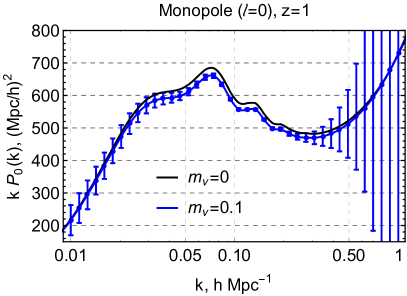
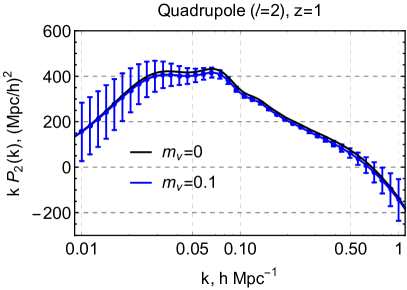
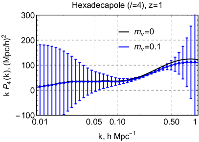
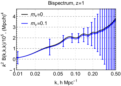
Figure 1: Monopole, quadrupole and hexadecapole of the one-loop galaxy power spectrum and the tree-level monopole bispectrum for the equilateral configuration at $z=1$: theoretical curves for $m_{\nu}=0.1$ eV (blue line), $m_{\nu}=0$ eV (black line), along with the mock data. The errorbars on short scales blow up because of the theoretical uncertainty added to the covariance. Note that the monopole power spectrum and bisepectrum increase at high momenta due to the strong shot noise contribution.

To generate the power spectrum and multipole datasets, we evaluate expressions (2.4,2.9) for the fiducial cosmology and bias parameters in each redshift bin. We consider wavenumbers spanning the range $0.01\,h\text{Mpc}^{-1}\leq k\leq 1\,h\text{Mpc}^{-1}$ and split them into 40 logarithmically spaced k-bins ($N_{k}=40$). Note that the choice of $k_{\text{max}}=1\leavevmode\nobreak\ h$/Mpc is arbitrary, our results do not depend on it by virtue of the theoretical error. Recall that the range of fundamental bins covers $k_{\rm f}\equiv 2\pi/V^{1/3}=(2.8-3.8)\times 10^{-3}\,h\text{Mpc}^{-1}$ depending on a particular redshift bin in the survey. We neglect the effects of the survey window function. They are sizable only on large scales (around $k_{\text{f}}$), which contain very little information compared to the mildly non-linear scales.

The mock bispectrum data were generated using the tree-level formulas for real and redshift spaces (2.22,2.25). For both analyses we set $k_{\rm min}=0.01\,h\text{Mpc}^{-1}$, $k_{\rm max}=0.5\,h\text{Mpc}^{-1}$ and split the corresponding momentum interval into 20 linearly spaced k-bins of width $\Delta k=0.026\,h\text{Mpc}^{-1}$ ($N_{k}=20$), which produced 825 different triangular configurations. For simplicity, we neglect binning effects both for the mock data and theoretical models.

In Fig. 1 we display the power spectrum multipoles and the equilateral isotropic bispectrum of our mock data at the mean redshift $z=1$ along with the errors representing the diagonal part of the covariance matrix. In each panel we show two theoretical curves corresponding to zero and fiducial neutrino masses. The error on large scales is dominated by sample variance, on short scales - by the theoretical uncertainty.

5 Results

In this section we present our results and discuss various effects that contribute to the cosmological parameter measurements from LSS [18]. We first discuss in detail the neutrino mass limits, and then focus on the parameters of the minimal $\Lambda$CDM.

Recall that the main effects of massive neutrinos on the linear dark-matter-baryon power spectrum is its uniform suppression for $k\gg k_{\text{nr}}$ ($k_{\text{nr}}$ is the comoving free-streaming wavenumber at the time when the neutrinos become non-relativistic),

$$\frac{P_{\mathrm{lin}}(k,z=0)^{m_{\nu}\neq 0}}{P_{\mathrm{lin}}(k,z=0)^{m_{\nu}=0}}\approx 1-6f_{\nu}\,.$$ (5.1)

The modes with $k\ll k_{\text{nr}}$ behave as if neutrinos were dark matter, and the matter power spectrum is the same as in the massless neutrino case. For small neutrino masses ($m_{\nu}\lesssim 100$ meV) the transition between these two asymptotics happens at large scales dominated by cosmic variance, which makes it hard to observe even with future surveys. At short scales where the statistical error reduces, the massive neutrino effect becomes almost indistinguishable from a simple reduction of the primordial power spectrum amplitude. However, the neutrino suppression has a non-trivial redshift dependence, which may help to break this degeneracy if several redshifts are combined in the analysis. The situation becomes more intricate if we consider galaxies, non-linearities and redshift-space distortions. To clearly illustrate different effects that impact the neutrino mass measurements, we start by the analysis of real space.

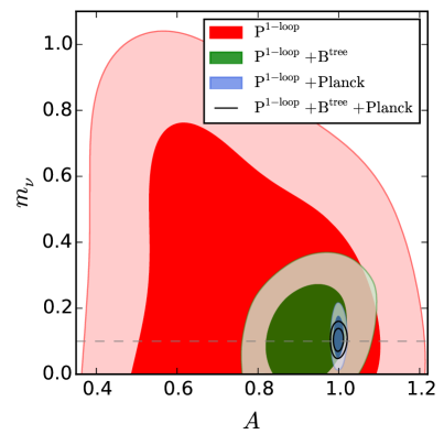
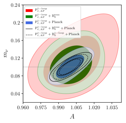
Figure 2: $1\sigma$ and $2\sigma$ contours in plane $m_{\nu}-A$ for the real space (left panel) and redshift space (right panel) analyses. $m_{\nu}$ is quoted in units of  eV. See also Tab. 4 for the marginalized constraints.

5.1 Real space

The results of our real space analysis are presented in the left panel of Fig. 2. For clarity, we show only the marginalized 2d distribution for $A$ and $m_{\nu}$. The marginalized 1-d constraints on neutrino masses and cosmological parameters are listed in the top panel of Tab. 4. Note that the value for the 1$\sigma$ neutrino mass error is approximate as the posterior distribution is quite non-Gaussian in the real space case.

We start with the pure power spectrum case. For galaxies in real space the situation is complicated by bias, which does not allow one to extract the amplitude of primordial fluctuations directly from the power spectrum normalization, which goes as $\propto Ab_{1}^{2}$ on large scales. The degeneracy between $A$ and $b_{1}$ may be partly broken by the loop corrections to the underlying dark matter density, which scale as $A^{2}b_{1}^{2}$. However, at one-loop order there also appear additional loop contributions due to the non-linear bias expansion, which are degenerate with the dark matter loops.

In principle, a non-trivial redshift dependence may help break the degeneracy between $A$ and $b_{1}$. However we treat the bias coefficients as nuisance parameters and marginalize over their time-dependence within our conservative analysis. Thus, we cannot probe the redshift evolution of the neutrino suppression. Therefore, the degeneracy between $A$ and $b_{1}$ is very strong, and once we marginalize over $b_{1}$, the neutrino mass remains largely unconstrained, see the red contour in the left panel of Fig. 2. We can rule out only very heavy neutrinos with $m_{\nu}\sim 0.5$ eV, whose effect on the matter power spectrum is significantly scale-dependent on mildly non-linear scales.

The situation greatly improves upon adding the tree-level bispectrum likelihood, see the green contour in the left panel of Fig. 2. The bispectrum amplitude scales like $A^{2}b_{1}^{3}$, which helps to break the notorious degeneracy between $A$ and $b_{1}$ present in the power spectrum. Still, the poor accuracy of amplitude and tilt measurements does not allow for a robust detection of the neutrino mass.

Once we add the Planck likelihood, it becomes a dominant source of the cosmological information, and helps reduce the errorbar on the neutrino masses down to $48$ meV for the joint power spectrum + bispectrum + Planck likelihood. This happens mainly because the Planck data fix the amplitude and tilt of the fluctuation spectrum. Since our Planck likelihood is not sensitive to the neutrino mass, our results suggest that a joint CMB + LSS analysis yields a large information gain crucial for a robust neutrino mass detection. In particular, the joint $\rm P^{\mathrm{1\text{-}loop}}+\rm B^{\mathrm{tree}}+\rm Planck$ constraints on $h$ and $\omega_{cdm}$ are much better than the Planck limits alone. This happens because the degeneracy direction in $h-\omega_{cdm}$ plane present in the LSS data is almost orthogonal to the degeneracy direction in the CMB data. We will return to this question shortly. However, by comparing the marginalized constraints from Planck alone and the joint $\rm P^{\mathrm{1\text{-}loop}}+\rm B^{\mathrm{tree}}+\rm Planck$ likelihoods one may notice that our LSS real-space data tighten the bounds on $n_{s}$, $\omega_{b}$ and $A$ only marginally.

Set	$10^{3}\,h$	$10^{2}\,A$	$10^{3}\,\omega_{cdm}$	$10^{4}\,\omega_{b}$	$10^{3}\,n_{s}$	$m_{\nu},\,\text{meV}$
Planck	15.2	0.9	1.4	1.6	4.2	$<260$
$\rm P^{\mathrm{1\text{-}loop}}$	37.4	18.9	13.8	38.1	62.2	$<510$
$\rm P^{\mathrm{1\text{-}loop}}\!+\!B^{\mathrm{tree}}$	19.1	7.2	7.3	19.5	23	$<210$
$\rm P^{\mathrm{1\text{-}loop}}\!+\!Planck$	1.7	0.9	0.7	1.2	3	$42$
$\rm P^{\mathrm{1\text{-}loop}}\!+\!B^{\mathrm{tree}}\!+\!Planck$	1	0.8	0.4	1.1	2.8	$22$
$\rm P_{\ell,nw}^{\mathrm{1\text{-}loop}}$	7.9	1.8	2.7	13.8	7.6	$55$
$\rm P_{\ell}^{\mathrm{1\text{-}loop}}$	7.7	1.7	2.7	9.3	6.5	$48$
$\rm P_{\rm\ell,\,AP}^{\mathrm{1\text{-}loop}}$	7.6	1.6	2.4	9.1	6.2	$38$
$\rm P_{\rm\ell,\,AP}^{\mathrm{1\text{-}loop}}\!+\!B_{0}^{\mathrm{tree}}$	5.5	1.1	2	6	4.6	$28$
$\rm P_{\rm\ell,\,AP}^{\mathrm{1\text{-}loop}}\!+\!Planck$	2	0.8	0.4	1.1	2.6	$17$
$\rm P_{\rm\ell,\,AP}^{\mathrm{1\text{-}loop}}\!+\!B_{0}^{\mathrm{tree}}\!+\!Planck$	0.9	0.7	0.3	1.1	2	$13$
$\rm P_{\rm\ell,\,AP}^{\mathrm{1\text{-}loop}}\!+\!B_{0}^{\mathrm{1\text{-}loop}}$	4.8	0.9	1.8	5.2	3.8	$23$
$\rm P_{\rm\ell,\,AP}^{\mathrm{1\text{-}loop}}\!+\!B_{0}^{\mathrm{1\text{-}loop}}\!+\!Planck$	0.8	0.6	0.3	1	1.8	$11$

Table 4: Marginalized $1\sigma$ errors for the cosmological parameters in the base $\Lambda$CDM with one massive neutrino (see Table 2) for different combinations of likelihoods. If the $1\sigma$ confidence limit on the neutrino mass overlaps with zero, we display a $68\%$ CL upper bound instead. We also show the constraints from a realistic Planck mock likelihood, which are in good agreement with the Planck 2018 legacy data [8].

5.2 Redshift space

To track the sources of improvement brought by the redshift space data we analyzed several different likelihoods that feature relevant physical effects separately. First, we study the impact of the BAO by analyzing a mock dataset without the BAO wiggles. Second, we scrutinize the information content of the one-loop anisotropic power spectrum with and without the AP effect. Third, we study different combinations of the power spectrum, tree-level bispectrum and Planck likelihoods. Finally, we perform a simplified unrealistic analysis of the one-loop power spectrum. Now we present all these case studies separately.

BAO and IR resummation. Massive neutrinos affect the size of the sound horizon at recombination [18]. Roughly speaking, this scale is imprinted in the matter power spectrum in two ways. First, it sets the frequency of the BAO wiggles and second, it defines the effective Jeans length for baryons, which suppress the short-scale part of the matter power before recombination. In this regard it is instructive to quantify how much information on the neutrino masses comes directly from the BAO wiggles. To this end we ran an MCMC power spectrum analysis for a mock datasample without the BAO wiggles. The details of this analysis are given in Appendix C, 1d marginalized limits are shown in the 6th line of Table 4. We found that the BAO decrease the error quite weakly, from $55\,\text{meV}$ to $48\,\text{meV}$. Our analysis suggests that the BAO impact notably only $\omega_{b}$ and $n_{s}$ measurements, whereas the improvement for other cosmological parameters is marginal. Nevertheless, we stress that an accurate description of the BAO feature by means of IR-resummation (see Sec. 2.3) is an essential part of any reliable full-shape measurement.

Redshift space distortions. RSD help improve the constrains in several ways. First, RSD break the degeneracy between $b_{1}$, $A$ and $n_{s}$ by allowing one to measure different multipoles. Since massive neutrinos produce a similar suppression in all power spectrum multipoles, $b_{1}$, $A$ and $n_{s}$ are not enough to simultaneously absorb this suppression in all multipoles at different redshifts. Second, the degeneracies between different bias coefficients in redshift space are partly broken because they enter the multipoles on different footing (see Eq. 2.9). These effects yield a significant improvement compared to the real space case reflected in Table 4.

Alcock-Paczynski effect. The AP test provides an additional probe of underling cosmology by mapping $H(z)$ and $D_{A}(z)$. Since all scales in a galaxy survey are measured in units of $\text{Mpc}/h$, the Hubble parameter drops out of the expressions for the AP effect, which turns out to be sensitive only to the total background matter density $\Omega_{m}$. Thus, the AP effect probes the background neutrino density fraction $\Omega_{\nu}$, which explains the improvement observed in Table 4. The AP test helps reduce the errorbar on the neutrino masses down to $38\,\text{meV}$. The precision gain for other cosmological parameters is more modest, which suggests that the AP geometric information is subdominant compared to the power spectrum shape.

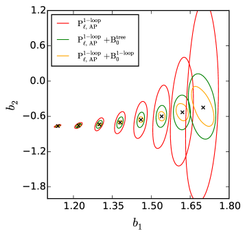
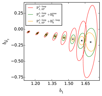
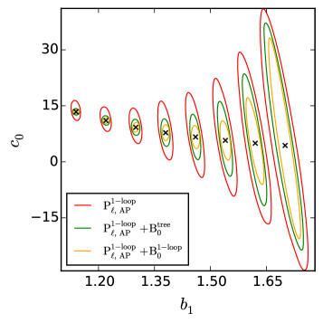
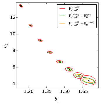
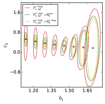
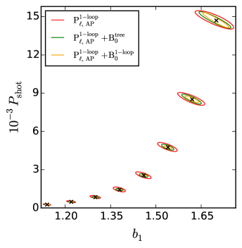
Figure 3: $1\sigma$ contours for bias parameters and RSD counterterm coefficients obtained for different combinations of the power spectrum and bispectrum likelihoods. Black crosses reflect the fiducial values listed in Table 3. The counterterm values $c_{i}$ are quoted in units [Mpc$/h]^{2}$, the shot noise $P_{\text{shot}}$ in units [Mpc$/h]^{3}$.

Planck likelihood. As anticipated, the neutrino mass constraints become significantly stronger upon adding the Planck likelihood, which allows one to define all standard cosmological parameters much better than the Euclid power spectrum data alone. Remarkably, the joint Euclid $+$ Planck likelihood constrains $\omega_{cdm}$ and $h$ much better than each of these likelihoods separately. This happens because LSS breaks the corresponding parameter degeneracy present in the CMB data. This effect will be discussed in more detail in Sec. 5.3.

As an additional cross-check, in Appendix F we reanalyze the LSS likelihoods in combination with a multivariate Gaussian approximation to the real Planck likelihood [8], in which case it effectively acts as a prior on the minimal cosmological parameters. We show that the use of the Gaussian approximation yields very similar results for the minimal parameters, but noticeably bigger errors on the neutrino mass as compared to the realistic mock likelihood. This implies that breaking the CMB degeneracies between $m_{\nu}$ and the cosmological parameters by the LSS data is a very important contribution to our eventual constraint on the neutrino mass.

Bispectrum. The main effect expected from the bispectrum is a more precise measurement of bias parameters. This is illustrated in Fig. 3, where we show the constraints on different bias parameters as a function of $b_{1}$, which can be used as a proxy for redshift. At large redshifts the contours are very wide because the loop corrections are sizable only in the high-$k$ tail, which is dominated by the shot noise. At low redshifts the effect of bias parameters and counterterms becomes more pronounced at lower wavenumbers and dominates over the noise, hence the contours shrink. One can see that the bispectrum substantially improves the constraints on $b_{2}$ and $b_{\mathcal{G}_{2}}$, while the gain for the counterterms is more modest.

Importantly, including the bispectrum tightens limits on the cosmological parameters. Regarding the neutrino masses, one can specifically emphasize much better measurements of the amplitude and tilt, which are comparable to the current Planck limits. Overall, the Euclid data alone are able to constrain the total neutrino mass with an errorbar of $28\,\text{meV}$. The main advantage of this constraint is that it entirely comes from Euclid data and does not utilize information from the CMB. Even so, this bound is competitive with that coming from the power spectrum $+$ Planck likelihoods without the bispectrum, see Table 4.

Including the power spectrum, bispectrum and the Planck likelihoods altogether reduces the errorbar on the neutrino masses down to $13\,\text{meV}$. The information gain of combining the Euclid survey and the CMB data in this case allows one to detect the fiducial neutrino mass $100$ meV at the $7.7\sigma$ significance. This constraint can also be interpreted as a forecast for the $4.6\sigma$ detection of the guaranteed minimal neutrino mass $60$ meV.

As far as the one-loop bispectrum is concerned, our over-optimistic (unrealistic) analysis with no new bias parameters shows that without the Planck data the constraints improve quite noticeably. However, if we add the Planck data, there is almost no difference between the tree-level and the one-loop bispectrum likelihoods. The interpretation of this result is straightforward: adding the tree-level bispectrum data breaks degeneracies between CMB and LSS, which results in a significant improvement. But once the degeneracy is broken, the gain from adding more of the bispectrum information is very modest. It would be interesting to understand to what extent the situation can change after taking into account higher-order multipole moments and the AP effect in the bispectrum, omitted in the present analysis.

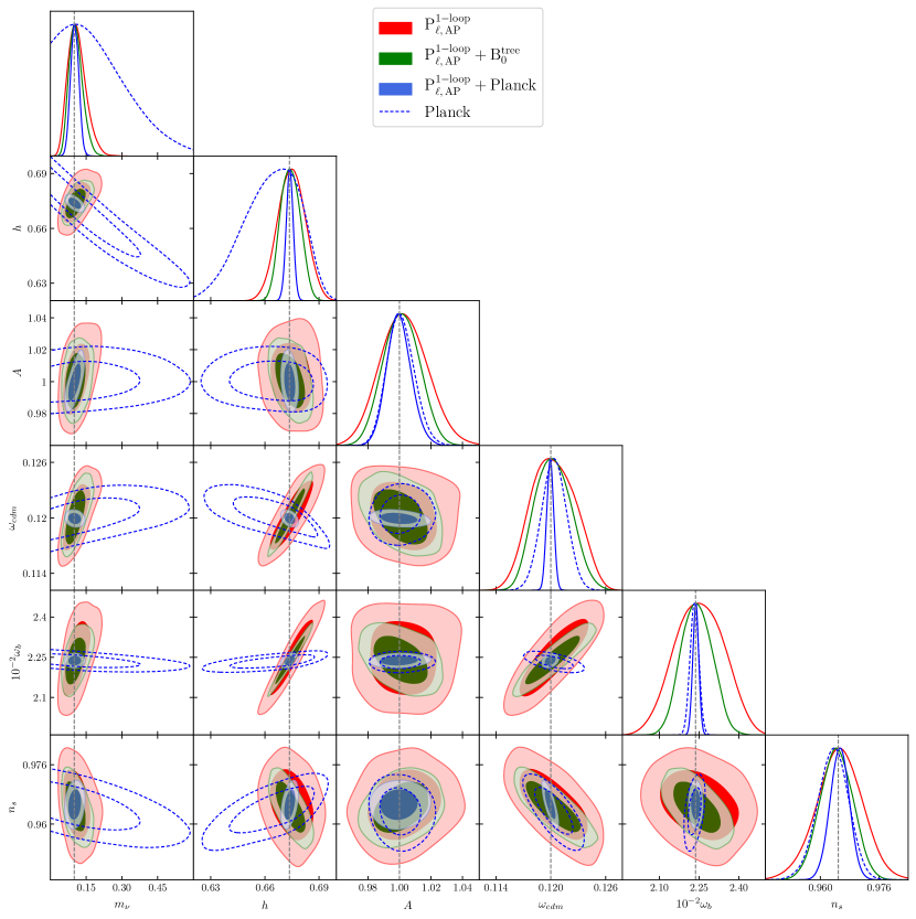
Figure 4: 2d posterior contours and non-normalized 1d marginalized distributions for the total neutrino mass $m_{\nu}$ in units $[\,\text{eV}]$ and other parameters of the base $\Lambda$CDM, see also Tab. 4 for the corresponding $1\sigma$ confidence limits. The filled and half-filled contours represent $68\%$ and $95\%$ confidence limits. The blue dashed lines correspond the Planck 2018 baseline results reproduced with the mock Planck likelihood.

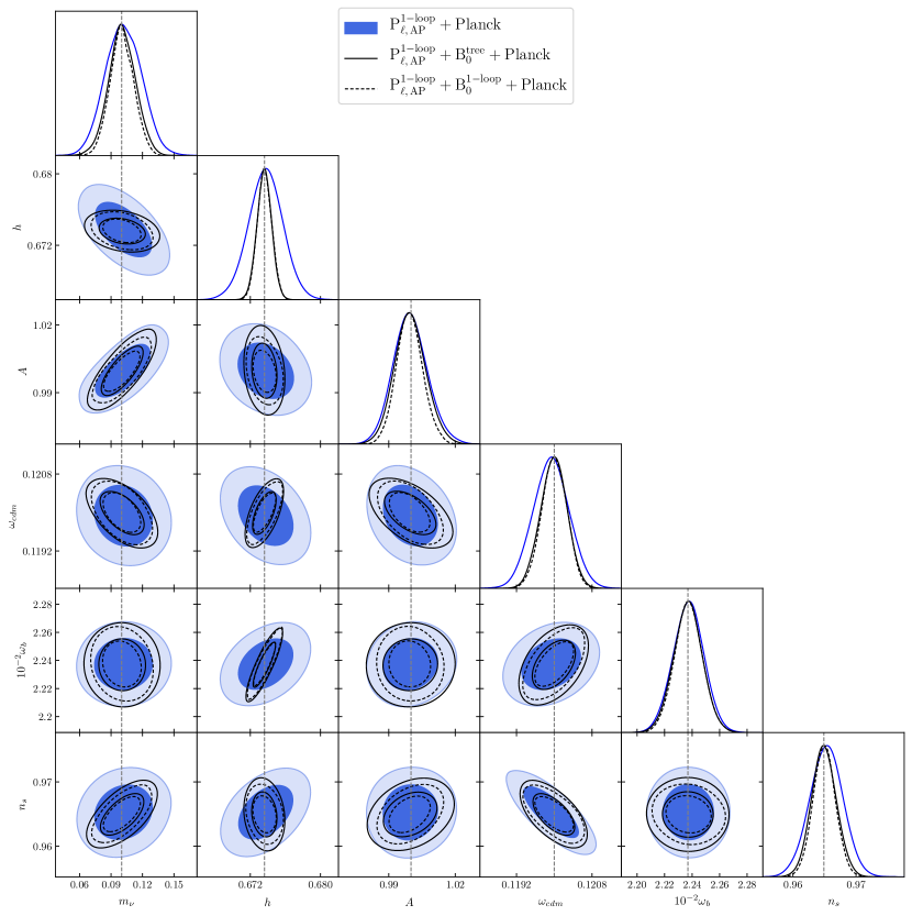
Figure 5: The 2d posterior contours and non-normalized 1d 2d posterior contours and non-normalized 1d marginalized distributions for the total neutrino mass $m_{\nu}$ in units $[\,\text{eV}]$ and other parameters of the base $\Lambda$CDM, see also Tab. 4 for the corresponding $1\sigma$ confidence limits. The filled and half-filled contours represent $68\%$ and $95\%$ confidence limits.

5.3 Cosmological parameters

Let us discuss now the constraints on the standard cosmological parameters. The corresponding triangle plots are displayed in Fig. 4 and Fig. 5. In Fig. 4 we show the posterior distributions for the power spectrum, power spectrum + bispectrum and power spectrum + Planck likelihoods, respectively in red, green and blue. The dashed blue line represents the Planck CMB-only constraints on the baseline $\Lambda$CDM with the varied neutrino mass (corresponding values are stated at the very top of Tab. 4). Fig. 5 shows a similar triangle plot for the combination of Planck and different LSS likelihoods: Planck + power spectrum (also shown in Fig. 4), Planck + power spectrum + tree-level bispectrum, and Planck + power spectrum + one-loop bispectrum (in which we unrealistically assumed that there are no additional bias parameters compared to the tree-level bispectrum). For compactness we do not show the contours for the bias parameters and counterterms.

One can observe sizable degeneracies between $h$, $\omega_{cdm}$ and $\omega_{b}$ in the RSD$+$AP power spectrum contours. These degeneracies can be readily understood from the fitting formulas for the power spectrum [147, 148, 149]. The shape of the linear matter spectrum expressed in units of Mpc$/h$ depends only on two scales:

$$k_{\text{eq}}=(7.46\cdot 10^{-2}\omega_{cb}/h)\,\,\,h\text{Mpc}^{-1}\,,$$ (5.2a)

$$r_{d}\simeq\frac{55.154\,{\rm e}^{-72.3(\omega_{\nu}+0.0006)^{2}}h}{\omega_{cb}^{0.25351}\omega_{b}^{0.12807}}\,\,\,\text{Mpc}/h\,,\quad\text{with}\quad\omega_{\nu}=\frac{m_{\nu}}{93.14\,\text{eV}}\,,$$ (5.2b)

which define its primary features: the equality peak, BAO wiggles and the effective Jeans length for baryons. Similarly to the case of the CMB spectrum, most of the degeneracy directions seen in Fig. 4 can be traced back to the locations of these features. The equality scale $k_{\text{eq}}$ controls the position of the power spectrum peak, while the sound horizon at the drag epoch sets the frequency of the BAO wiggles along with the effective Jean scale for baryons, which slow down short-scale clustering before recombination [18]. The amount of this suppression is set by the ratio ${\omega_{b}}/{\omega_{cb}}$. This ratio also controls the amplitude of the BAO wiggles relative to the broadband. Note that in units of Mpc both scales $r_{d}$ and $k_{\text{eq}}$ depend only on $\omega_{b}$, $\omega_{cdm}$ and $\omega_{\nu}$. If we could measure the power spectrum in units of Mpc, these physical densities would be the only parameters controlling the power spectrum shape.

It is useful to understand the degeneracies seen in the 2d marginalized contours of Fig. 4. Let us first focus on the pair $\omega_{cdm}-h$. Upon marginalyzing over $\omega_{b}$, the constancy of the equality and BAO scales in units of Mpc/$h$ fixes the combinations $\omega_{cdm}h^{-1}$ and $\omega_{cdm}h^{-4}$. Their geometrical mean roughly corresponds to the observed degeneracy direction $\omega_{cdm}h^{-2}$. The direction $\omega^{0.5}_{b}/\omega_{cdm}$ seen in the corresponding panel is likely to be a combination of $\omega_{b}/\omega_{cdm}$ and the sound horizon (5.2b). As for the obtained degeneracy direction $\omega_{b}h^{-3.3}$, its origin roots in the constancy of $r_{d}$ in units of Mpc/$h$, which leads to $\omega^{0.38}_{b}h^{-1}$ upon marginalization of (5.2b) over $\omega_{cdm}$. Note that $n_{s}$ has sizable degeneracies with $\omega_{cdm}$, $h$ and $\omega_{b}$ in the LSS data. These degeneracies reflect the fact that the Jeans-like suppression of the matter power spectrum by the baryons can be partly compensated by a proper adjustment of the tilt.

We observe that the Euclid power spectrum data alone (red contours) is competitive with the Planck alone (blue dashed contours) in terms of the amplitude, the Hubble parameter and the tilt, whereas $\omega_{cdm}$ and $\omega_{b}$ are still measured much worse. By comparing the green and red contours in Fig. 4, one sees that the bispectrum data have almost the same degeneracies as the power spectrum one, but its inclusion noticeably improves the constraints on all cosmological parameters. In particular, by combining power spectrum and bispectrum data (green contours) one can notice that the Hubble parameter and tilt measurements reach the precision comparable with the recent Planck results whereas the amplitude accuracy even surpasses the Planck limit. Still, even in this case the Planck CMB data remain much better for $\omega_{cdm}$ and $\omega_{b}$. All in all, the improvement seen in Fig. 4 implies that the redshift space bispectrum contains rich information about cosmological parameters.

The bounds on $h$, $\omega_{b}$ and $\omega_{cdm}$ ameliorate significantly upon combining the Euclid power spectrum and the Planck likelihoods (blue contours). The key observation here is that LSS measures best the combination $\omega_{cdm}h^{-2}$, which is quite orthogonal to well-known CMB degeneracy related to the angular size of the acoustic horizon $\omega_{cdm}h$. The two degeneracy directions cut each other almost at the right angle leaving us with very narrow residual projections onto the $\omega_{cdm}$ and $h$ planes in Fig. 4. The resulting errors on $\omega_{cdm}$ and $h$, for instance, shrink by factors of 4.7 and 18 compared to the current Planck limit for the $\Lambda$CDM with the varied neutrino mass. A similar situation takes place for the $\omega_{cdm}-\omega_{b}$ and $\omega_{b}-h$ pairs, although the gain is slightly more modest in these cases. Remarkably, the eventual measurement of the Hubble constant from the combination of Planck and future LSS surveys will reach a $0.1\%$ precision, which will be important for elucidating the nature of the so-called “Hubble tension”, see e.g. [150] and references therein.

Overall, we conclude that synergy between the CMB and LSS data is essential to robustly measure the neutrino masses and cosmological parameters from future surveys.

5.4 Comparison with previous studies

There have been many forecasts on the neutrino mass and cosmological parameter measurements with a future galaxy spectroscopic surveys [67, 19, 62, 68, 69, 63, 22, 70, 64, 71, 73]. In this Section we discuss a few selected works that have a significant overlap with our study.

Our work can be seen as a continuation of the approach put forward in Ref. [19]. This work pointed out for the first time that the theoretical error method is more efficient for the large-scale structure data analysis than the use of the momentum cutoff $k_{\text{max}}$. There are three main improvements between this study and our work. First, Ref. [19] uses a somewhat simplified theoretical model for the matter power spectrum. It is based on the HALOFIT fitting formula for the non-linear matter power spectrum of dark matter, and features only linear bias and redshift-space distortions (the Kaiser formula applied to the HALOFIT). However, it includes a correction due to spectroscopic redshift error, which has the same function form as our redshift-space counterterms. Second, Ref. [19] considers two theoretical errors: one due to an imperfect description of massive neutrinos with the HALOFIT (this error is assumed to be correlated), and the other one due to overall non-linear clustering uncertainties (this error is conservatively assumed to be uncorrelated). In contrast, the error of our neutrino treatment is taken into account on the same footing as the other two-loop uncertainties, which are correlated as dictated by perturbation theory. Third, the analysis of Ref. [19] did not include the bispectrum. However, this work performed a full MCMC analysis and took into account the Alcock-Paczynski effect. Despite the mentioned methodological differences, our constraints are in good agreement with those obtained in Ref. [19] and its recent follow-ups [20, 22]. We believe that this happens because (i) the HALOFIT does capture the leading non-linear contributions, (ii) the non-linear bias coefficients present in our analysis get partly fixed by the bispectrum information, (iii) the counterterms present in our study have the same functional form as corrections due to spectroscopic redshift errors, and hence produce very similar effects on parameter space after marginalization. Overall, the good agreement between our paper and Refs. [19, 20, 22] indicates the consistency of the theoretical error framework and its robustness against setup variations.

Recently, the theoretical error formalism was revisited in the context of perturbation theory in Ref. [62]. This reference studied the impact of the theoretical error on the future neutrino mass and non-Gaussianity constraints by means of a Fisher matrix analysis of the galaxy power spectrum and bispectrum in real space. Our work can be seen as a straightforward generalization of Ref. [62] to the redshift space case. Compared to that reference, we run a full MCMC analysis and perform an exact evaluation of the one-loop power spectrum and tree-level bispectrum of redshift-space galaxies. Importantly, the analysis of Ref. [62] was done only in real space, and hence it misses important information from the velocity field, which enters through redshift-space distortions. Our study shows that taking into account this information dramatically improves the neutrino mass measurements.

Finally, let us discuss the relation between our work and a recent Euclid forecast on the cosmological constraints with the redshift-space bispectrum [49]. This paper performed a Fisher matrix forecast for the power spectrum and bispectrum of Euclid galaxies in redshift space for $\Lambda$CDM and extended dark energy models. The main conclusion of this paper is that the redshift-space bispectrum does not significantly improve the constraints on the cosmological parameters, both in combination with the power spectrum and with the joint power spectrum + Planck CMB likelihood. On the one hand, our analysis agrees with Ref. [49] in that the addition of the bispectrum to the power spectrum likelihood does not dramatically improve the constraints on the parameters of the minimal $\Lambda$CDM. On other other hand, we found a notable improvement for the neutrino mass, which was not considered in Ref. [49]. This result holds true for the combination of the LSS and the Planck CMB data, in which case the bispectrum also significantly improves the measurement of $h$ (in part by breaking the CMB degeneracy between $m_{\nu}$ and $h$). Moreover, our analysis of the LSS likelihood without the CMB data yielded somewhat stronger constrains on the cosmological parameters compared to those presented in Ref. [49]. This improvement calls for a more detailed comparison.

Although Ref. [49] uses an identical survey specification and a very similar theoretical model for tree-level the bispectrum (modulo IR resummation), there are several differences. First, Ref. [49] uses a conservative momentum cutoff $k_{\text{max}}=0.15\leavevmode\nobreak\ h$/Mpc for all redshift bins, whereas the theoretical error allows us to go to much larger wavenumbers, especially at high redshifts. Second, Ref. [49] employs the linear model for the redshift-space power spectrum, supplemented with an exponential fingers-of-God damping. In this approach the non-linear bias parameters are present only in the tree-level bispectrum, whereas in our work both the one-loop power spectrum and the tree-level bispectrum share the same bias coefficients $b_{2}$ and $b_{\mathcal{G}_{2}}$. Thus, these parameters are constrained from the two statistics simultaneously, which yields more cosmological information in the combined analysis. Besides, the one-loop power spectrum has a stronger response to a variation of cosmological parameters as compared to linear theory, and hence its inclusion tightens the constraints by itself. We illustrate these points in Appendix E. We believe that these effects resulted in somewhat tighter constraints compared to those presented in Ref. [49].

It should be pointed out that Ref. [49] features some important improvements compared to our study. First, it properly takes into account higher multipole moments of the redshift space bispectrum and the binning effects, which are ignored in our work. Importantly, it shows that not considering higher moments beyond the monopole bispectrum leads to a significant loss of information. Second, it scrutinizes the impact of the covariance between the power spectrum and the bispectrum, and different prescriptions for the stochastic noise. Finally, Ref. [49] analyzes the minimal $\Lambda$CDM along with extended dark energy models while in our analysis we restrict ourselves only to the base $\Lambda$CDM with massive neutrinos.

6 Conclusion and Outlook

We have presented a forecast for the cosmological parameter and neutrino mass measurement with a Euclid-like spectroscopic survey mock dataset. Our analysis contains several improvements compared to previous studies.

We use a complete analytical model for the power spectrum and bispectrum, which includes non-linear galaxy bias and redshift space distortions. First, we calculate explicit one-loop perturbation theory power spectra for the underlying matter field, which should be contrasted with the HALOFIT semi-analytic formula [151, 152] adopted in some previous studies. Second, we rigorously take into account the non-linear evolution of BAO. Third, we use the general non-linear biasing prescription and do not make any assumptions about the values and time-dependence of the corresponding bias coefficients. Fourth, we consider the non-linear redshift-space mapping which goes beyond the linear Kaiser formula. We parametrize various short-scale effects (e.g. fingers-of-God and baryonic feedback) by means of counterterms, for which we also allow arbitrary values and time-dependence. This way we avoid possible biases that might be introduced by simplified phenomenological prescriptions, e.g. the fingers-of-God exponential damping. Another important aspect of our analysis is the bispectrum, which notably improves the constraints on cosmological parameters. Our baseline theoretical model thus consists of the one-loop power spectrum and the tree-level bispectrum and can readily be applied to data analysis.

We make use of the MCMC technique and evaluate the non-linear power spectrum and bispectrum for each sampled set of cosmological parameters. We explicitly include the correlated theoretical error in our likelihoods. This error is based on estimates for higher-order loop corrections that are omitted in our theory calculations. Adding the theoretical error to the covariance matrix is equivalent to marginalizing over the shape of higher order non-linearities. This makes our predictions insensitive to the choice of the momentum cutoff scale $k_{\text{max}}$ commonly used in the previous LSS studies.

We show that even under most conservative assumptions on the galaxy bias, redshift-space distortions and non-linear physics, the future galaxy clustering data alone will be able to deliver satisfactory constrains on cosmological parameters and the sum of neutrino masses. Specifically, by using the combination of the power spectrum and bispectrum one will be able to probe the neutrino mass with an errorbar of $28\,\text{meV}$. By adding the CMB data from the Planck satellite, the error can be reduced down to $13\,\text{meV}$. This forecasts the detection of the minimal total neutrino mass with 4.6$\sigma$ (7.7$\sigma$) significance in the case of the direct (inverted) hierarchy. Our results are summarized in Fig. 6.

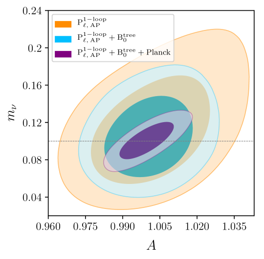
Figure 6: Posterior $1\sigma$ and $2\sigma$ contours in the $m_{\nu}-A(\equiv A_{s}/A_{s,\text{fid}})$ plane for the following likelihoods: one-loop power spectrum only (orange), one-loop power spectrum + tree-level bispectrum monopole (blue), one-loop power spectrum + tree-level bispectrum monopole + Planck (violet). $m_{\nu}$ is quoted in  eV.

It seems very unlikely that we will have no information on the values and time-dependence of the bias parameters and RSD counterterms by the time when the future LSS data are gathered. The most direct way is to obtain these priors from realistic mock catalogs. As far as the bias coefficients are concerned, their values can be estimated from the galaxy-galaxy lensing cross-correlation [153], or some semi-analytic models, e.g. the peak-background split (see [42] and references therein). Using these priors may drastically improve our conservative limits which were obtained under very agnostic assumptions about the properties of the Euclid galaxy sample.

There are several directions in which our study can be ameliorated. First, one can perform a more accurate analysis of the redshift space bispectrum that would include higher multipole moments, the Alcock-Paczynski effect, and a more general treatment of stochastic contributions. Second, one can extend the analysis to the case of the two-loop power spectrum and one-loop bispectrum. In that case one would have to consistently take into account non-Gaussian contributions to the covariance matrices and the cross-covariance between the power spectrum and the bispectrum. Third, it would be important to see how our results can be affected by instrumental uncertainties of a Euclid-like survey. Fourth, one has to verify our assumptions on the theoretical errors with N-body simulations. Fifth, one could make a similar analysis for other combinations of upcoming CMB and LSS surveys. Another interesting exploration venue is a forecast for non-minimal cosmological models, e.g. dynamical dark energy. We leave these tasks for future work.

Appendix A Explicit expressions for galaxy power spectrum multipoles

Let us start with the bias loop corrections to the real space galaxy power spectrum,

$$\begin{split}&{\cal I}_{\delta^{2}}(k)=2\int_{\bf q}F_{2}({\bf q},{\bf k}-{\bf q})P_{\text{lin}}(|{\bf k}-{\bf q}|)P_{\text{lin}}(q)\,,\\ &{\cal I}_{\mathcal{G}_{2}}(k)=2\int_{\bf q}\sigma^{2}({\bf q},{\bf k}-{\bf q})F_{2}({\bf q},{\bf k}-{\bf q})P_{\text{lin}}(|{\bf k}-{\bf q}|)P_{\text{lin}}(q)\,,\\ &{\cal F}_{\mathcal{G}_{2}}(k)=4P_{\text{lin}}(k)\int_{\bf q}\sigma^{2}({\bf q},{\bf k}-{\bf q})F_{2}({\bf q},{\bf k}-{\bf q})P_{\text{lin}}(q)\,,\\ &{\cal I}_{\delta^{2}\delta^{2}}(k)=2\int_{\bf q}P_{\text{lin}}(|{\bf k}-{\bf q}|)P_{\text{lin}}(q)-2\int_{\bf q}P^{2}_{\text{lin}}(q)\,,\\ &{\cal I}_{\mathcal{G}_{2}\mathcal{G}_{2}}(k)=2\int_{\bf q}\sigma^{4}({\bf q},{\bf k}-{\bf q})P_{\text{lin}}(|{\bf k}-{\bf q}|)P_{\text{lin}}(q)\,,\\ &{\cal I}_{\delta^{2}\mathcal{G}_{2}}(k)=2\int_{\bf q}\sigma^{2}({\bf q},{\bf k}-{\bf q})P_{\text{lin}}(|{\bf k}-{\bf q}|)P_{\text{lin}}(q)\,,\end{split}$$ (A.1)

where $\sigma^{2}({\bf k}_{1},{\bf k}_{2})=({\bf k}_{1}\cdot{\bf k}_{2})^{2}/(k_{1}^{2}k_{2}^{2})-1$, and $F_{2}$ is the standard SPT quadratic density kernel [25],

$$F_{2}({\bf k}_{1},{\bf k}_{2})=\frac{5}{7}+\frac{1}{2}\frac{({\bf k}_{1}\cdot{\bf k}_{2})}{k_{1}k_{2}}\left(\frac{k_{1}}{k_{2}}+\frac{k_{2}}{k_{1}}\right)+\frac{2}{7}\frac{({\bf k}_{1}\cdot{\bf k}_{2})^{2}}{k_{1}^{2}k_{2}^{2}}\,.$$ (A.2)

In what follows we will also use the SPT velocity kernels $G_{n}$. The galaxy power spectrum in redshift space is given by

$$\begin{split}P_{g}(k,\mu)=&Z^{2}_{1}({\bf k})P_{\text{lin}}(k)+2\int_{{\bf q}}Z^{2}_{2}({\bf q},{\bf k}-{\bf q})P_{\text{lin}}(|{\bf k}-{\bf q}|)P_{\text{lin}}(q)\\ &+6Z_{1}({\bf k})P_{\text{lin}}(k)\int_{{\bf q}}Z_{3}({\bf q},-{\bf q},{\bf k})P_{\text{lin}}(q)\\ &-2\tilde{c}_{0}k^{2}P_{\text{lin}}(k)-2\tilde{c}_{2}f\mu^{2}k^{2}P_{\text{lin}}(k)-2\tilde{c}_{4}f^{2}\mu^{4}k^{2}P_{\text{lin}}(k)+P_{\text{shot}}\,,\end{split}$$ (A.3)

where the redshift space kernels are given by

$$Z_{1}({\bf k})=b_{1}+f\mu^{2}\,,$$ (A.4a)

$$Z_{2}({\bf k}_{1},{\bf k}_{2})=\frac{b_{2}}{2}+b_{\mathcal{G}_{2}}\left(\frac{({\bf k}_{1}\cdot{\bf k}_{2})^{2}}{k_{1}^{2}k_{2}^{2}}-1\right)+b_{1}F_{2}({\bf k}_{1},{\bf k}_{2})+f\mu^{2}G_{2}({\bf k}_{1},{\bf k}_{2})$$

$$\qquad\qquad\quad\leavevmode\nobreak\ \leavevmode\nobreak\ +\frac{f\mu k}{2}\left(\frac{\mu_{1}}{k_{1}}(b_{1}+f\mu_{2}^{2})+\frac{\mu_{2}}{k_{2}}(b_{1}+f\mu_{1}^{2})\right)\,,$$ (A.4b)

$$Z_{3}({\bf k}_{1},{\bf k}_{2},{\bf k}_{3})=2b_{\Gamma_{3}}\left[\frac{({\bf k}_{1}\cdot({\bf k}_{2}+{\bf k}_{3}))^{2}}{k_{1}^{2}({\bf k}_{2}+{\bf k}_{3})^{2}}-1\right]\big{[}F_{2}({\bf k}_{2},{\bf k}_{3})-G_{2}({\bf k}_{2},{\bf k}_{3})\big{]}$$

$$\quad+b_{1}F_{3}({\bf k}_{1},{\bf k}_{2},{\bf k}_{3})+f\mu^{2}G_{3}({\bf k}_{1},{\bf k}_{2},{\bf k}_{3})+\frac{(f\mu k)^{2}}{2}(b_{1}+f\mu_{1}^{2})\frac{\mu_{2}}{k_{2}}\frac{\mu_{3}}{k_{3}}$$

$$\quad+f\mu k\frac{\mu_{3}}{k_{3}}\left[b_{1}F_{2}({\bf k}_{1},{\bf k}_{2})+f\mu^{2}_{12}G_{2}({\bf k}_{1},{\bf k}_{2})\right]+f\mu k(b_{1}+f\mu^{2}_{1})\frac{\mu_{23}}{k_{23}}G_{2}({\bf k}_{2},{\bf k}_{3})$$

$$\quad+b_{2}F_{2}({\bf k}_{1},{\bf k}_{2})+2b_{\mathcal{G}_{2}}\left[\frac{({\bf k}_{1}\cdot({\bf k}_{2}+{\bf k}_{3}))^{2}}{k_{1}^{2}({\bf k}_{2}+{\bf k}_{3})^{2}}-1\right]F_{2}({\bf k}_{2},{\bf k}_{3})+\frac{b_{2}f\mu k}{2}\frac{\mu_{1}}{k_{1}}$$

$$\quad+b_{\mathcal{G}_{2}}f\mu k\frac{\mu_{1}}{k_{1}}\left[\frac{({\bf k}_{2}\cdot{\bf k}_{3})^{2}}{k_{2}^{2}k_{3}^{2}}-1\right]\,,$$ (A.4c)

where ${\bf k}={\bf k}_{1}+{\bf k}_{2}+{\bf k}_{3}$ and the kernel $Z_{3}$ must be symmetrized over its arguments. The net expressions for the multipoles of the power spectrum model (A.3) are obtained upon averaging over $\mu=({\bf k}\cdot{\bf z})/k$ weighed with the appropriate Legendre polynomials. As for the counterterms, we use the following basis:

$$\begin{split}&P_{0,\nabla^{2}\delta}(k)=-k^{2}\cdot\left(\frac{b_{1}^{2}f^{2}}{3}+\frac{2b_{1}f^{3}}{5}+\frac{f^{4}}{7}\right)P_{\text{lin}}(k)\,,\\ &P_{2,\nabla^{2}\delta}(k)=-k^{2}\cdot\left(\frac{2b_{1}^{2}f^{2}}{3}+\frac{8b_{1}f^{3}}{7}+\frac{10f^{4}}{21}\right)P_{\text{lin}}(k)\,,\\ &P_{4,\nabla^{2}\delta}(k)=-k^{2}\cdot\frac{8f^{2}}{35}P_{\text{lin}}(k)\,,\end{split}$$ (A.5)

in which case $c_{0}$ and $c_{2}$ correspond directly to the short-scale velocity dispersion $\sigma^{2}_{v}$, see (3.10).

Appendix B Gaussian covariance matrices for redshift space power spectrum and bispectrum

The Gaussian covariance matrix for redshift-space power spectrum multipoles reads

$$\begin{split}C_{k_{i}k_{j}}^{(\ell_{1}\ell_{2})}=\frac{2}{N_{k}}\frac{(2\ell_{1}+1)}{2}\left(2\ell_{2}+1\right)\int_{-1}^{1}d\mu\,L_{\ell_{1}}(\mu)L_{\ell_{2}}(\mu)\left[P_{g}(k_{i},\mu)+\frac{1}{\bar{n}_{g}}\right]^{2}\delta_{ij}.\end{split}$$ (B.1)

Doing the $\mu$-integral and expressing everything in terms of the multipoles one obtains

$$\begin{split}&C^{(00)}_{k_{i}k_{j}}=\frac{2}{N_{k}}\left(P_{0}^{2}+\frac{1}{5}P_{2}^{2}+\frac{1}{9}P_{4}^{2}\right)\delta_{ij}\,,\\ &C^{(02)}_{k_{i}k_{j}}=\frac{2}{N_{k}}\left(2P_{0}P_{2}+\frac{2}{7}P_{2}^{2}+\frac{4}{7}P_{2}P_{4}+\frac{100}{693}P_{4}^{2}\right)\delta_{ij}\,,\\ &C^{(04)}_{k_{i}k_{j}}=\frac{2}{N_{k}}\left(\frac{18}{35}P^{2}_{2}+2P_{0}P_{4}+\frac{40}{77}P_{2}P_{4}+\frac{162}{1001}P_{4}^{2}\right)\delta_{ij}\,,\\ &C^{(22)}_{k_{i}k_{j}}=\frac{2}{N_{k}}\left(5P_{0}^{2}+\frac{20P_{0}P_{2}}{7}+\frac{20P_{0}P_{4}}{7}+\frac{15P_{2}^{2}}{7}+\frac{120P_{2}P_{4}}{77}+\frac{8945P_{4}^{2}}{9009}\right)\delta_{ij}\,,\\ &C^{(24)}_{k_{i}k_{j}}=\frac{2}{N_{k}}\left(\frac{36P_{0}P_{2}}{7}+\frac{200P_{0}P_{4}}{77}+\frac{108P_{2}^{2}}{77}+\frac{3578P_{2}P_{4}}{1001}+\frac{900P_{4}^{2}}{1001}\right)\delta_{ij}\,,\\ &C^{(44)}_{k_{i}k_{j}}=\frac{2}{N_{k}}\left(9P_{0}^{2}+\frac{360P_{0}P_{2}}{77}+\frac{2916P_{0}P_{4}}{1001}+\frac{16101P_{2}^{2}}{5005}+\frac{3240P_{2}P_{4}}{1001}+\frac{42849P_{4}^{2}}{17017}\right)\delta_{ij}\,,\end{split}$$ (B.2)

where we introduced the number of modes $N_{k}=V{k^{2}dk}/{(4\pi^{2})}$. Eq. (B.1) generalizes to the isotropic redshift space bispectrum,

$$C^{\ell=0}_{TT^{\prime}}=\frac{\left(2\pi\right)^{3}}{V(z)}\frac{\pi s_{123}}{dk_{1}dk_{2}dk_{3}}\frac{\delta_{TT^{\prime}}}{k_{1}k_{2}k_{3}}\frac{1}{4\pi}\int_{0}^{2\pi}d\phi\int_{0}^{\pi}d\omega\,\sin\omega\,\prod_{a=1}^{3}\left[P_{g}(k_{a},\mu_{a})+\frac{1}{\bar{n}_{g}}\right]\,.$$ (B.3)

Choosing the coordinate system as in Ref. [109], it is trivial to obtain the final expression for the redshift space covariance matrix. We leave it as an exercise to the reader.

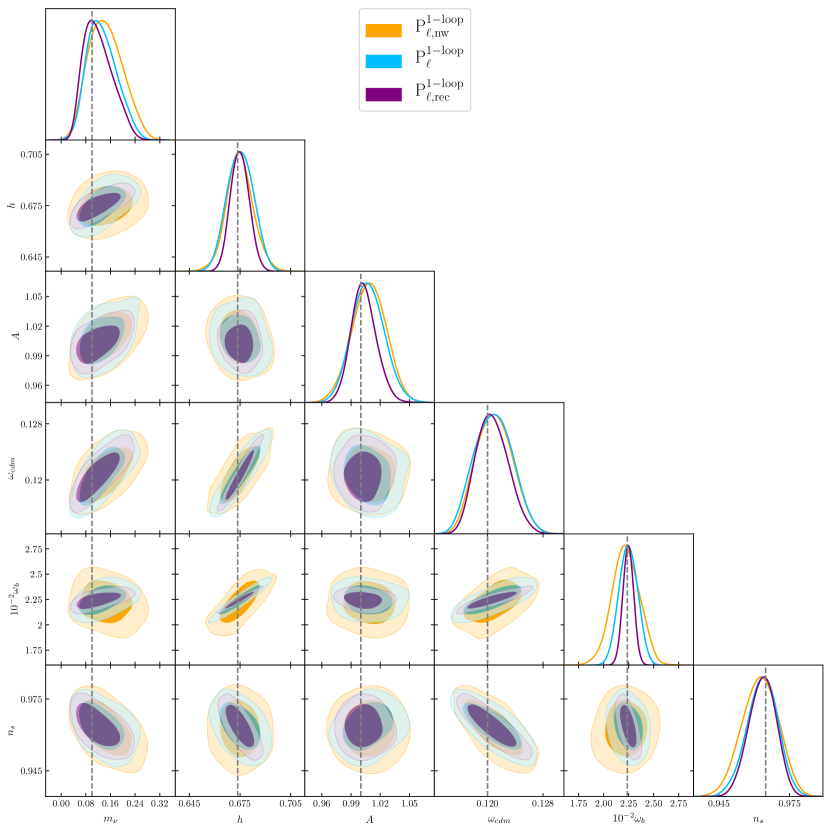
Figure 7: $1\sigma$ and $2\sigma$ contours, see Tab. 5 for the 1d marginalized limits.

Appendix C Information content of baryon acoustic oscillations

To quantify the information gain from the BAO we analyzed mock power spectrum likelihoods simulated for two extreme situations: the fully damped and totally undamped BAO wiggles. Using our definition of the damping factor in Sec. 2.3, they formally correspond to the following two cases:

$$\Sigma^{2}\to\infty\,,\quad\text{(nw)}\,,$$ (C.1a)

$$\Sigma^{2}\to 0\,,\quad\text{(rec)}\,,$$ (C.1b)

In the first case there are no BAO wiggles whatsoever. This case should be contrasted with the BAO-only measurements (done e.g. in Ref. [66]), in which one throws away the broadband information and only fits the BAO wiggles. Our analysis does exactly the opposite: we throw away the BAO wiggles and fit the remaining shape. A similar approach was previously used in Ref. [155]. Note that when fitting the non-wiggly mock data we also remove the BAO wiggles in our theoretical templates using the same wiggly-smooth decomposition algorithm.

The second case is equivalent to using BAO reconstruction [156, 157, 158, 159, 160, 161], a data-driven method that aims at restoring the linear amplitude of the BAO wiggles. This method strongly distorts the broadband part such that its cosmological information is typically discarded. Although the standard BAO reconstruction techniques [156, 157] do not fully recover the linear BAO wiggles [66], it is, in principle, possible in more sophisticated approaches [161]. In this regard, our second case can be though of as a joint analysis of the full-shape data and the optimally reconstructed BAO. This case should show the importance of the high-$k$ wiggles, which are normally diluted by large-scale bulk flows.

The outcome of our analysis is presented in Fig. 7 and Table 5. There we show the results for the non-wiggly redshift-space power spectrum $P^{\text{1-loop}}_{\ell,\,\text{nw}}$, the reference one-loop power from our main analysis $P^{\text{1-loop}}_{\ell}$, and the power spectrum with fully reconstructed BAO wiggles $P^{\text{1-loop}}_{\ell,\,\text{rec}}$.

Let us first focus on the first case (nw). We observe the biggest change in $\omega_{b}$ and $n_{s}$. This is explained by the argument that without the BAO wiggles $\omega_{b}$ is measured through the suppression of the power spectrum at short scales, which can be partly compensated by the tilt. The presence of the BAO wiggles allows one to break this degeneracy. Remarkably, the absence of the BAO feature does not degrade the constraints on $h$, which is responsible for the geometric distance information. This shows that the power spectrum shape would be a powerful tool to extract cosmological parameters even if the BAO were absent in the matter distribution.

Now let us consider the mock combined analysis with the reconstructed BAO (rec). This analysis captures information from the high-$k$ BAO wiggles, which benefits from smaller errors compared to the low-$k$ BAO used in our main analysis. As a result, the parameter constrains improve quite sizable, e.g. the errorbar on $h$ reduces by $\sim 30\%$. This points out the importance of the BAO reconstruction, which can complement cosmological parameter measurements from the power-spectrum and bispectrum shape.

Set	$10^{3}\,h$	$10^{2}\,A$	$10^{3}\,\omega_{c}$	$10^{4}\,\omega_{b}$	$10^{3}\,n_{s}$	$m_{\nu},\,\text{meV}$
$\rm P_{\ell,nw}^{\mathrm{1\text{-}loop}}$	7.9	1.8	2.7	13.8	7.6	$55$
$\rm P_{\ell}^{\mathrm{1\text{-}loop}}$	7.7	1.7	2.7	9.3	6.5	$48$
$\rm P_{\ell,rec}^{\mathrm{1\text{-}loop}}$	5.4	1.2	2.2	5.3	5.6	$45$

Table 5: Marginalized $1\sigma$ error for the cosmological parameters in $\Lambda$CDM model with one massive neutrino, see Table 2. We show results for the non-wiggle (smooth) one-loop redshift space power spectrum (first line), the reference power spectrum with realistically damped BAO wiggles (second line), and the power spectrum with fully undamped (reconstructed) BAO wiggles (third line).

Appendix D Results for the theoretical error with a strong Fingers-of-God effect

Set	$10^{3}\,h$	$10^{2}\,A$	$10^{3}\,\omega_{c}$	$10^{4}\,\omega_{b}$	$10^{3}\,n_{s}$	$m_{\nu},\,\text{meV}$
$\rm P_{\rm\ell,\,AP}^{\mathrm{1\text{-}loop}}\!+\!B_{0}^{\mathrm{tree}}(FoG+2L)$	9.4	3	3.5	10	10.7	$50$
$\rm P_{\rm\ell,\,AP}^{\mathrm{1\text{-}loop}}\!+\!B_{0}^{\mathrm{tree}}(2L)$	5.5	1.1	2	6	4.6	$28$

Table 6: Marginalized $1\sigma$ error for the cosmological parameters in $\Lambda$CDM model with a massive neutrino, see Table 2 for definitions. We display results for the one-loop redshift space power spectrum and the tree-level bispectrum likelihoods with the baseline theoretical error (corresponding to dark matter two loops - 2L) and the theoretical error that includes both the loop contribution and a template for the strong Fingers-of-God effect (FoG).

Our main analysis was performed for the theoretical error template dominated by the two-loop corrections due to dark matter clustering. This template does not contain higher-order corrections generated by fingers-of-God, which is motivated by several arguments. First, fingers-of-God were found to be small in mock catalogs of Euclid-type galaxies [116, 119]. Second, the fingers-of-God effect is mostly produced by the velocity dispersion of the satellite galaxies. But the satellites can be removed from the catalog when computing the power spectrum [103]. Central galaxies have much smaller velocity dispersion and its contribution is of the same order as the two-loop corrections due to dark matter clustering. Third, fingers-of-God plague only the line-of-side modes, while the modes with the wavevectors with other directions are much less affected by them. Building the redshift-space wedges and throwing away the angular bins with $|\mu|\sim 1$ allows one to remove fingers-of-God while retaining most of the information encoded in the power spectrum. In this case the residual theoretical error of the redshift-space wedges should indeed be dominated by the dark matter two loops.

From these arguments it is clear that there are ways to extract cosmological information regardless of the strength of fingers-of-God. However, it is curios to see how much the constraints will degrade if one naively analyzes the power spectrum multipoles in the presence of strong fingers-of-God. To this end we reanalyzed our mock data with a new theoretical error covariance that contains both envelops (4.11) and (4.10). We chose the next-to-leading order contribution (4.11) to be universal for all multipole moments, as dictated by the redshift-space mapping, and assumed $\sigma_{v}=5\,\text{Mpc}/h$ for all multipole moments in (4.11).

The results obtained for the power spectrum + bispectrum mock likelihoods are presented in Tab. 6. One can see that using the conservative template for the theoretical error covariance degrades constraints on all cosmological parameters roughly by a factor of 2. In particular, the uncertainty of neutrino mass measurement worsens to $50\,\,\text{meV}$. However, our result shows that the effect of the strong fingers-of-God is not catastrophic. Even in this case the constraints on cosmological parameters from the LSS data alone are competitive with the Planck-alone CMB measurements.

Appendix E Analysis with a sharp momentum cutoff

Set	$10^{3}\,h$	$10^{2}\,A$	$10^{3}\,\omega_{c}$	$10^{4}\,\omega_{b}$	$10^{3}\,n_{s}$	$m_{\nu},\,\text{meV}$
$\rm P_{\rm\ell,AP}^{\mathrm{1\text{-}loop}}\!+\!B_{0}^{\mathrm{tree}}\leavevmode\nobreak\ (k_{max})$	22	5.6	7.8	24.9	20.2	$<206$
$\rm P_{\rm\ell}^{\mathrm{tree}}\!+\!B_{0}^{\mathrm{tree}}\leavevmode\nobreak\ (k_{max})$	38.6	6.9	14.4	42.4	25.5	$<254$
$\rm P_{\rm\ell,\,AP}^{\mathrm{1\text{-}loop}}\!+\!B_{0}^{\mathrm{tree}}\leavevmode\nobreak\ (TE)$	5.5	1.1	2	6	4.6	$28$

Table 7: Marginalized $1\sigma$ error for the cosmological parameters in $\Lambda$CDM model with one massive neutrino, see Table 2, considering one-loop/linear redshift space power spectrum and tree-level bispectrum with the sharp cutoff $k_{\text{max}}=0.15\,h\text{Mpc}^{-1}$. For comparison, we also show the results of our baseline analysis with the theoretical error, $\rm P_{\rm\ell,\,AP}^{\mathrm{1\text{-}loop}}\!+\!B_{0}^{\mathrm{tree}}\leavevmode\nobreak\ (TE)$. If the $1\sigma$ constraint on neutrino mass is consistent with zero, we provide an upper bound of the $68\%$ confidence region.

In this Appendix we present several additional analyses that are aimed to (i) reveal how much the theoretical error formalism improves over the sharp cutoff approach, and (ii) quantify the difference between the use of the linear and one-loop power spectrum in LSS forecasts.

To show the difference between our baseline analysis and the $k_{\text{max}}$ results we construct new one-loop power spectrum and tree-level bispectrum mock likelihoods without the theoretical error and with a sharp momentum cut at $k_{\rm max}=0.15\,h\text{Mpc}^{-1}$. This choice is motivated by previous analysis of the BOSS DR12 galaxy clustering [53] and the Euclid forecast of Ref. [49]. Note that this choice is somewhat conservative because perturbation theory predictions are, in fact, reliable for bigger wavenumbers, and even more so at high redshifts to be probed by Euclid-like surveys.

For the rest, we follow the methodology of our baseline analysis. In particular, we use the same binning for the power spectrum (see Sec. 4.5 for more detail), whereas for the mock bispectrum data we use $k_{\rm min}=0.01\,h\text{Mpc}^{-1}$, $k_{\rm max}=0.15\,h\text{Mpc}^{-1}$ splitting the corresponding momentum interval into 10 linearly spaced k-bins of width $\Delta k=0.016\,h\text{Mpc}^{-1}$. Our results are presented in Tab. 7 (first line, $\rm P_{\rm\ell,AP}^{\mathrm{1\text{-}loop}}\!+\!B_{0}^{\mathrm{tree}}\leavevmode\nobreak\ (k_{max})$). One can see that constraints on all cosmological parameters degrade dramatically. In particular, the $1\sigma$-bound on the total neutrino mass becomes very loose, $m_{\nu}<206\,\,\text{meV}$ ($68\%$ CL) which is comparable to the current Planck-only limit [8]. This result suggests that the use of the theoretical error approach allows one to extract significantly more information from the mildly non-linear scales compared to an analysis with a conservative sharp $k_{\text{max}}$ cutoff.

Let us now discuss the impact of the power spectrum modeling on the forecasts for future LSS surveys, some of which use the linear model with the fingers-of-God damping, see e.g. [49]. Two important comments are in order here. First, the use of the tree-level expressions both for the power spectrum and bispectrum leads to the loss of cosmological information. The reason is that the tree-level matter power spectrum model ignores the non-linear bias coefficients which are present in the tree-level bispectrum. However, the non-linear bias is a characteristic of the whole density field and hence should be treated on the same footing both in the power spectrum and bispectrum at any given order in perturbation theory. This implies that the power spectrum must necessarily be computed at the one-loop order if one analyzes the tree-level bispectrum. Since the tree-level bispectrum and the one-loop power spectrum share the same bias parameters $b_{2}$ and $b_{\mathcal{G}_{2}}$, they are better constrained in the joint analysis, which allows one to extract more cosmological information. Second, the use of the one-loop matter power spectrum can improve the constraints by itself as compared to a forecast based on linear theory. Indeed, since $P^{\text{1-loop}}\propto P_{\mathrm{lin}}^{2}$, the one-loop power spectrum has a twice bigger response to a variation of cosmological parameters. Moreover, the one-loop power spectrum introduces new redshift-dependent shape modifications that are absent in linear theory. In general, the one-loop correction is smaller than the linear part, so this effect is not expected to be very dramatic unless one is interested in subtle phenomena like neutrino masses.

Given these reasons, we expect the effects discussed above to be relevant for our forecast. In order to study their impact we generated new power spectrum and bispectrum mock likelihoods, in which both these statistics are computed only at the tree level, without the theoretical error, and with a sharp momentum cut at $k_{\rm max}=0.15\,h\text{Mpc}^{-1}$. To match the previous forecasts, we do not include the AP effect and IR resummation in our model. Besides, we prefer not to include the Finger-of-God exponential damping in the linear power spectrum model, which should formally be taken into account along with the one-loop corrections omitted here. The results are shows in Tab. 7 (second line, $\rm P_{\rm\ell}^{\mathrm{tree}}\!+\!B_{0}^{\mathrm{tree}}\leavevmode\nobreak\ (k_{max})$). Overall, our results are consistent with those of Ref. [49]. One observes that for the same choice of $k_{\text{max}}$ the use of the one-loop matter power spectrum leads to notably better results compared to the forecast based on the linear matter power spectrum.

Appendix F Analysis with a Gaussian approximation to the Planck likelihood

In this Appendix we present the results for the analyses which use the multivariate Gaussian approximation to the Planck likelihood. The Planck posterior distribution is substantially asymmetric when the massive neutrino are included into the fit [8], and hence the Gaussian approximation does not accurately capture actual confidence regions [121]. Given this reason, we focus only on the covariance matrix extracted from the Planck baseline analysis that fixed the neutrino mass to the minimal value $60$ meV. In other words, our Gaussian likelihood approximation does not include massive neutrinos, and consequently does not capture their effect on the CMB data whatsoever. The use of this covariance matrix is, strictly speaking, inconsistent. However, it is still meaningful for the following two goals: (i) Demonstrate the robustness of our mock Planck likelihood used in the baseline analysis and (ii) Get an idea on the cosmological constrains which can be obtained from LSS if we use the CMB priors only on the cosmological parameters and not the neutrino mass, which is curios in light of the “lensing tension” present in the Planck CMB data [8].

Set	$10^{3}\,h$	$10^{2}\,A$	$10^{3}\,\omega_{cdm}$	$10^{4}\,\omega_{b}$	$10^{3}\,n_{s}$	$m_{\nu},\,\text{meV}$
Planck Gaussian (Planck G)	5.4	1.4	1.2	1.5	4.2	$-$
$\rm P^{\mathrm{1\text{-}loop}}\!+\!Planck\leavevmode\nobreak\ G$	1.3	1.4	0.3	1.2	3.1	$<226$
$\rm P^{\mathrm{1\text{-}loop}}\!+\!B^{\mathrm{tree}}\!+\!Planck\leavevmode\nobreak\ G$	0.8	1.3	0.2	1.1	3	$48$
$\rm P_{\rm\ell,\,AP}^{\mathrm{1\text{-}loop}}\!+\!Planck\leavevmode\nobreak\ G$	1.8	1	0.4	1.1	2.9	$24$
$\rm P_{\rm\ell,\,AP}^{\mathrm{1\text{-}loop}}\!+\!B_{0}^{\mathrm{tree}}\!+\!Planck\leavevmode\nobreak\ G$	0.8	0.9	0.2	1.1	1.9	$19$
$\rm P_{\rm\ell,\,AP}^{\mathrm{1\text{-}loop}}\!+\!B_{0}^{\mathrm{1\text{-}loop}}\!+\!Planck\leavevmode\nobreak\ G$	0.8	0.7	0.2	1	1.7	$17$

Table 8: Marginalized $1\sigma$ errors for the cosmological parameters in $\Lambda$CDM with one massive neutrino (see Table 2) for different combinations of likelihoods. For comparison, we also show current Planck limits on the parameters of the base $\Lambda$CDM with a fixed minimal neutrino mass, hence the corresponding error is omitted in the topmost row. If $1\sigma$ posterior contour of neutrino mass overlaps with zero, we show an upper bound of corresponding $68\%$ CL limit.

All in all, we downloaded Markov chains that sampled the cosmological parameters of the base_plikHM_TTTEEE_lowl_lowE_lensing likelihood from the Planck Legacy Archive and computed the covariance matrix for a subset of cosmological parameters $h,\omega_{cdm},\omega_{b},n_{s},A,\tau$. Then we used the Gaussian likelihood with this covariance matrix to derive constraints for the same combinations of likelihoods as in our baseline analysis. The results are displayed in Table 8. The first observation is that the errorbars on the cosmological parameters are somewhat different in the full mock and the Gaussian Planck likelihoods without the LSS data. However, the difference reduces when we add the LSS likelihoods. On the one hand, we observe a very good agreement between the CMB+LSS runs with the Gaussian approximation and the realistic mock Planck likelihood for the parameters of the minimal $\Lambda$CDM. On the other hand, the Gaussian likelihood worsens significantly the constraints on the neutrino masses, which is a result of neglecting the correlations between $m_{\nu}$ and other cosmological parameters present in the CMB data, e.g. $m_{\nu}$ and $h$. Our results represent an important consistency check proving that the information gain indeed comes from breaking of the degeneracies between the LSS and CMB.

References

- [1] X. Qian and P. Vogel, Neutrino Mass Hierarchy, Prog. Part. Nucl. Phys. 83 (2015) 1 [1505.01891].
- [2] Particle Data Group collaboration, M. Tanabashi et al., Review of Particle Physics, Phys. Rev. D98 (2018) 030001.
- [3] V. M. Lobashev, The search for the neutrino mass by direct method in the tritium beta-decay and perspectives of study it in the project KATRIN, Nucl. Phys. A719 (2003) 153.
- [4] C. Kraus et al., Final results from phase II of the Mainz neutrino mass search in tritium beta decay, Eur. Phys. J. C40 (2005) 447 [hep-ex/0412056].
- [5] K. Eitel, Direct neutrino mass experiments, Nucl. Phys. Proc. Suppl. 143 (2005) 197.
- [6] Troitsk collaboration, V. N. Aseev et al., An upper limit on electron antineutrino mass from Troitsk experiment, Phys. Rev. D84 (2011) 112003 [1108.5034].
- [7] KATRIN collaboration, M. Aker et al., An improved upper limit on the neutrino mass from a direct kinematic method by KATRIN, 1909.06048.
- [8] Planck collaboration, N. Aghanim et al., Planck 2018 results. VI. Cosmological parameters, 1807.06209.
- [9] N. Palanque-Delabrouille et al., Neutrino masses and cosmology with Lyman-alpha forest power spectrum, JCAP 1511 (2015) 011 [1506.05976].
- [10] B. Bolliet, T. Brinckmann, J. Chluba and J. Lesgourgues, Including massive neutrinos in thermal Sunyaev Zeldovich power spectrum and cluster counts analyses, 1906.10359.
- [11] H. Gil-Marín, L. Verde, J. Noreña, A. J. Cuesta, L. Samushia, W. J. Percival et al., The power spectrum and bispectrum of SDSS DR11 BOSS galaxies – II. Cosmological interpretation, Mon. Not. Roy. Astron. Soc. 452 (2015) 1914 [1408.0027].
- [12] BOSS collaboration, F. Beutler et al., The clustering of galaxies in the SDSS-III Baryon Oscillation Spectroscopic Survey: signs of neutrino mass in current cosmological data sets, Mon. Not. Roy. Astron. Soc. 444 (2014) 3501 [1403.4599].
- [13] A. J. Cuesta, V. Niro and L. Verde, Neutrino mass limits: robust information from the power spectrum of galaxy surveys, Phys. Dark Univ. 13 (2016) 77 [1511.05983].
- [14] BOSS collaboration, S. Alam et al., The clustering of galaxies in the completed SDSS-III Baryon Oscillation Spectroscopic Survey: cosmological analysis of the DR12 galaxy sample, Mon. Not. Roy. Astron. Soc. 470 (2017) 2617 [1607.03155].
- [15] BOSS collaboration, J. N. Grieb et al., The clustering of galaxies in the completed SDSS-III Baryon Oscillation Spectroscopic Survey: Cosmological implications of the Fourier space wedges of the final sample, Mon. Not. Roy. Astron. Soc. 467 (2017) 2085 [1607.03143].
- [16] A. Upadhye, Neutrino mass and dark energy constraints from redshift-space distortions, JCAP 1905 (2019) 041 [1707.09354].
- [17] W. Hu, D. J. Eisenstein and M. Tegmark, Weighing neutrinos with galaxy surveys, Phys. Rev. Lett. 80 (1998) 5255 [astro-ph/9712057].
- [18] J. Lesgourgues and S. Pastor, Massive neutrinos and cosmology, Phys. Rept. 429 (2006) 307 [astro-ph/0603494].
- [19] B. Audren, J. Lesgourgues, S. Bird, M. G. Haehnelt and M. Viel, Neutrino masses and cosmological parameters from a Euclid-like survey: Markov Chain Monte Carlo forecasts including theoretical errors, JCAP 1301 (2013) 026 [1210.2194].
- [20] M. Archidiacono, T. Brinckmann, J. Lesgourgues and V. Poulin, Physical effects involved in the measurements of neutrino masses with future cosmological data, JCAP 1702 (2017) 052 [1610.09852].
- [21] T. Sprenger, M. Archidiacono, T. Brinckmann, S. Clesse and J. Lesgourgues, Cosmology in the era of Euclid and the Square Kilometre Array, JCAP 1902 (2019) 047 [1801.08331].
- [22] T. Brinckmann, D. C. Hooper, M. Archidiacono, J. Lesgourgues and T. Sprenger, The promising future of a robust cosmological neutrino mass measurement, JCAP 1901 (2019) 059 [1808.05955].
- [23] M. M. Ivanov, M. Simonovic and M. Zaldarriaga, Cosmological Parameters from the BOSS Galaxy Power Spectrum, 1909.05277.
- [24] EUCLID collaboration, R. Laureijs et al., Euclid Definition Study Report, 1110.3193.
- [25] F. Bernardeau, S. Colombi, E. Gaztanaga and R. Scoccimarro, Large scale structure of the universe and cosmological perturbation theory, Phys. Rept. 367 (2002) 1 [astro-ph/0112551].
- [26] M. Crocce and R. Scoccimarro, Nonlinear Evolution of Baryon Acoustic Oscillations, Phys. Rev. D77 (2008) 023533 [0704.2783].
- [27] S. Pueblas and R. Scoccimarro, Generation of Vorticity and Velocity Dispersion by Orbit Crossing, Phys. Rev. D80 (2009) 043504 [0809.4606].
- [28] D. Baumann, A. Nicolis, L. Senatore and M. Zaldarriaga, Cosmological Non-Linearities as an Effective Fluid, JCAP 1207 (2012) 051 [1004.2488].
- [29] D. Blas, S. Floerchinger, M. Garny, N. Tetradis and U. A. Wiedemann, Large scale structure from viscous dark matter, JCAP 1511 (2015) 049 [1507.06665].
- [30] L. Senatore and M. Zaldarriaga, The IR-resummed Effective Field Theory of Large Scale Structures, JCAP 1502 (2015) 013 [1404.5954].
- [31] Z. Vlah, U. Seljak, M. Y. Chu and Y. Feng, Perturbation theory, effective field theory, and oscillations in the power spectrum, JCAP 1603 (2016) 057 [1509.02120].
- [32] D. Blas, M. Garny, M. M. Ivanov and S. Sibiryakov, Time-Sliced Perturbation Theory II: Baryon Acoustic Oscillations and Infrared Resummation, JCAP 1607 (2016) 028 [1605.02149].
- [33] T. Baldauf, M. Mirbabayi, M. Simonović and M. Zaldarriaga, Equivalence Principle and the Baryon Acoustic Peak, Phys. Rev. D92 (2015) 043514 [1504.04366].
- [34] M. M. Ivanov and S. Sibiryakov, Infrared Resummation for Biased Tracers in Redshift Space, JCAP 1807 (2018) 053 [1804.05080].
- [35] E. Noda, M. Peloso and M. Pietroni, A Robust BAO Extractor, JCAP 1708 (2017) 007 [1705.01475].
- [36] D. Blas, M. Garny, M. M. Ivanov and S. Sibiryakov, Time-Sliced Perturbation Theory for Large Scale Structure I: General Formalism, JCAP 1607 (2016) 052 [1512.05807].
- [37] J. J. M. Carrasco, M. P. Hertzberg and L. Senatore, The Effective Field Theory of Cosmological Large Scale Structures, JHEP 09 (2012) 082 [1206.2926].
- [38] M. Lewandowski, A. Perko and L. Senatore, Analytic Prediction of Baryonic Effects from the EFT of Large Scale Structures, JCAP 1505 (2015) 019 [1412.5049].
- [39] P. McDonald and A. Roy, Clustering of dark matter tracers: generalizing bias for the coming era of precision LSS, JCAP 0908 (2009) 020 [0902.0991].
- [40] L. Senatore, Bias in the Effective Field Theory of Large Scale Structures, JCAP 1511 (2015) 007 [1406.7843].
- [41] M. Mirbabayi, F. Schmidt and M. Zaldarriaga, Biased Tracers and Time Evolution, JCAP 1507 (2015) 030 [1412.5169].
- [42] V. Desjacques, D. Jeong and F. Schmidt, Large-Scale Galaxy Bias, Phys. Rept. 733 (2018) 1 [1611.09787].
- [43] T. Lazeyras, C. Wagner, T. Baldauf and F. Schmidt, Precision measurement of the local bias of dark matter halos, JCAP 1602 (2016) 018 [1511.01096].
- [44] T. Lazeyras and F. Schmidt, A robust measurement of the first higher-derivative bias of dark matter halos, 1904.11294.
- [45] T. Lazeyras and F. Schmidt, Beyond LIMD bias: a measurement of the complete set of third-order halo bias parameters, JCAP 1809 (2018) 008 [1712.07531].
- [46] M. M. Abidi and T. Baldauf, Cubic Halo Bias in Eulerian and Lagrangian Space, JCAP 1807 (2018) 029 [1802.07622].
- [47] H. Gil-Marín, C. Wagner, J. Noreña, L. Verde and W. Percival, Dark matter and halo bispectrum in redshift space: theory and applications, JCAP 1412 (2014) 029 [1407.1836].
- [48] F.-S. Kitaura, H. Gil-Marín, C. Scoccola, C.-H. Chuang, V. Müller, G. Yepes et al., Constraining the halo bispectrum in real and redshift space from perturbation theory and non-linear stochastic bias, Mon. Not. Roy. Astron. Soc. 450 (2015) 1836 [1407.1236].
- [49] V. Yankelevich and C. Porciani, Cosmological information in the redshift-space bispectrum, Mon. Not. Roy. Astron. Soc. 483 (2019) 2078 [1807.07076].
- [50] D. Karagiannis, A. Lazanu, M. Liguori, A. Raccanelli, N. Bartolo and L. Verde, Constraining primordial non-Gaussianity with bispectrum and power spectrum from upcoming optical and radio surveys, Mon. Not. Roy. Astron. Soc. 478 (2018) 1341 [1801.09280].
- [51] H. Gil-Marín, J. Noreña, L. Verde, W. J. Percival, C. Wagner, M. Manera et al., The power spectrum and bispectrum of SDSS DR11 BOSS galaxies – I. Bias and gravity, Mon. Not. Roy. Astron. Soc. 451 (2015) 539 [1407.5668].
- [52] H. Gil-Marín, W. J. Percival, L. Verde, J. R. Brownstein, C.-H. Chuang, F.-S. Kitaura et al., The clustering of galaxies in the SDSS-III Baryon Oscillation Spectroscopic Survey: RSD measurement from the power spectrum and bispectrum of the DR12 BOSS galaxies, Mon. Not. Roy. Astron. Soc. 465 (2017) 1757 [1606.00439].
- [53] BOSS collaboration, F. Beutler et al., The clustering of galaxies in the completed SDSS-III Baryon Oscillation Spectroscopic Survey: Anisotropic galaxy clustering in Fourier-space, Mon. Not. Roy. Astron. Soc. 466 (2017) 2242 [1607.03150].
- [54] BOSS collaboration, S. Satpathy et al., The clustering of galaxies in the completed SDSS-III Baryon Oscillation Spectroscopic Survey: On the measurement of growth rate using galaxy correlation functions, Mon. Not. Roy. Astron. Soc. 469 (2017) 1369 [1607.03148].
- [55] C. Alcock and B. Paczynski, An evolution free test for non-zero cosmological constant, Nature 281 (1979) 358.
- [56] J. E. McEwen, X. Fang, C. M. Hirata and J. A. Blazek, FAST-PT: a novel algorithm to calculate convolution integrals in cosmological perturbation theory, JCAP 1609 (2016) 015 [1603.04826].
- [57] M. Schmittfull and Z. Vlah, FFT-PT: Reducing the two-loop large-scale structure power spectrum to low-dimensional radial integrals, Phys. Rev. D94 (2016) 103530 [1609.00349].
- [58] X. Fang, J. A. Blazek, J. E. McEwen and C. M. Hirata, FAST-PT II: an algorithm to calculate convolution integrals of general tensor quantities in cosmological perturbation theory, JCAP 1702 (2017) 030 [1609.05978].
- [59] M. Simonović, T. Baldauf, M. Zaldarriaga, J. J. Carrasco and J. A. Kollmeier, Cosmological perturbation theory using the FFTLog: formalism and connection to QFT loop integrals, JCAP 1804 (2018) 030 [1708.08130].
- [60] A. J. S. Hamilton, Uncorrelated modes of the nonlinear power spectrum, Mon. Not. Roy. Astron. Soc. 312 (2000) 257 [astro-ph/9905191].
- [61] D. Blas, J. Lesgourgues and T. Tram, The Cosmic Linear Anisotropy Solving System (CLASS) II: Approximation schemes, JCAP 1107 (2011) 034 [1104.2933].
- [62] T. Baldauf, M. Mirbabayi, M. Simonović and M. Zaldarriaga, LSS constraints with controlled theoretical uncertainties, 1602.00674.
- [63] A. Boyle and E. Komatsu, Deconstructing the neutrino mass constraint from galaxy redshift surveys, JCAP 1803 (2018) 035 [1712.01857].
- [64] A. Boyle, Understanding the neutrino mass constraints achievable by combining CMB lensing and spectroscopic galaxy surveys, 1811.07636.
- [65] F. Beutler, M. Biagetti, D. Green, A. Slosar and B. Wallisch, Primordial Features from Linear to Nonlinear Scales, 1906.08758.
- [66] BOSS collaboration, F. Beutler et al., The clustering of galaxies in the completed SDSS-III Baryon Oscillation Spectroscopic Survey: baryon acoustic oscillations in the Fourier space, Mon. Not. Roy. Astron. Soc. 464 (2017) 3409 [1607.03149].
- [67] M. Takada, E. Komatsu and T. Futamase, Cosmology with high-redshift galaxy survey: neutrino mass and inflation, Phys. Rev. D73 (2006) 083520 [astro-ph/0512374].
- [68] M. LoVerde, Neutrino mass without cosmic variance, Phys. Rev. D93 (2016) 103526 [1602.08108].
- [69] A. Raccanelli, L. Verde and F. Villaescusa-Navarro, Biases from neutrino bias: to worry or not to worry?, Mon. Not. Roy. Astron. Soc. 483 (2019) 734 [1704.07837].
- [70] S. Vagnozzi, T. Brinckmann, M. Archidiacono, K. Freese, M. Gerbino, J. Lesgourgues et al., Bias due to neutrinos must not uncorrect’d go, JCAP 1809 (2018) 001 [1807.04672].
- [71] G. Parimbelli, M. Viel and E. Sefusatti, On the degeneracy between baryon feedback and massive neutrinos as probed by matter clustering and weak lensing, JCAP 1901 (2019) 010 [1809.06634].
- [72] S. Mishra-Sharma, D. Alonso and J. Dunkley, Neutrino masses and beyond- LCDM cosmology with LSST and future CMB experiments, Phys. Rev. D97 (2018) 123544 [1803.07561].
- [73] D. Copeland, A. Taylor and A. Hall, Towards determining the neutrino mass hierarchy: weak lensing and galaxy clustering forecasts with baryons and intrinsic alignments, 1905.08754.
- [74] T. Baldauf, L. Mercolli, M. Mirbabayi and E. Pajer, The Bispectrum in the Effective Field Theory of Large Scale Structure, JCAP 1505 (2015) 007 [1406.4135].
- [75] R. E. Angulo, S. Foreman, M. Schmittfull and L. Senatore, The One-Loop Matter Bispectrum in the Effective Field Theory of Large Scale Structures, JCAP 1510 (2015) 039 [1406.4143].
- [76] M. Pietroni, Flowing with Time: a New Approach to Nonlinear Cosmological Perturbations, JCAP 0810 (2008) 036 [0806.0971].
- [77] M. Fasiello and Z. Vlah, Nonlinear fields in generalized cosmologies, Phys. Rev. D94 (2016) 063516 [1604.04612].
- [78] D. Blas, M. Garny, T. Konstandin and J. Lesgourgues, Structure formation with massive neutrinos: going beyond linear theory, JCAP 1411 (2014) 039 [1408.2995].
- [79] F. Führer and Y. Y. Y. Wong, Higher-order massive neutrino perturbations in large-scale structure, JCAP 1503 (2015) 046 [1412.2764].
- [80] L. Senatore and M. Zaldarriaga, The Effective Field Theory of Large-Scale Structure in the presence of Massive Neutrinos, 1707.04698.
- [81] S. Saito, M. Takada and A. Taruya, Impact of massive neutrinos on nonlinear matter power spectrum, Phys. Rev. Lett. 100 (2008) 191301 [0801.0607].
- [82] R. Ruggeri, E. Castorina, C. Carbone and E. Sefusatti, DEMNUni: Massive neutrinos and the bispectrum of large scale structures, JCAP 1803 (2018) 003 [1712.02334].
- [83] R. de Belsunce and L. Senatore, Tree-Level Bispectrum in the Effective Field Theory of Large-Scale Structure extended to Massive Neutrinos, JCAP 1902 (2019) 038 [1804.06849].
- [84] F. Villaescusa-Navarro, S. Bird, C. Pena-Garay and M. Viel, Non-linear evolution of the cosmic neutrino background, JCAP 1303 (2013) 019 [1212.4855].
- [85] M. LoVerde and M. Zaldarriaga, Neutrino clustering around spherical dark matter halos, Phys. Rev. D89 (2014) 063502 [1310.6459].
- [86] H. Dupuy and F. Bernardeau, On the importance of nonlinear couplings in large-scale neutrino streams, JCAP 1508 (2015) 053 [1503.05707].
- [87] C.-T. Chiang, W. Hu, Y. Li and M. Loverde, Scale-dependent bias and bispectrum in neutrino separate universe simulations, Phys. Rev. D97 (2018) 123526 [1710.01310].
- [88] C.-T. Chiang, M. LoVerde and F. Villaescusa-Navarro, First detection of scale-dependent linear halo bias in -body simulations with massive neutrinos, Phys. Rev. Lett. 122 (2019) 041302 [1811.12412].
- [89] F. Villaescusa-Navarro, F. Marulli, M. Viel, E. Branchini, E. Castorina, E. Sefusatti et al., Cosmology with massive neutrinos I: towards a realistic modeling of the relation between matter, haloes and galaxies, JCAP 1403 (2014) 011 [1311.0866].
- [90] E. Castorina, E. Sefusatti, R. K. Sheth, F. Villaescusa-Navarro and M. Viel, Cosmology with massive neutrinos II: on the universality of the halo mass function and bias, JCAP 1402 (2014) 049 [1311.1212].
- [91] M. Costanzi, F. Villaescusa-Navarro, M. Viel, J.-Q. Xia, S. Borgani, E. Castorina et al., Cosmology with massive neutrinos III: the halo mass function andan application to galaxy clusters, JCAP 1312 (2013) 012 [1311.1514].
- [92] E. Castorina, C. Carbone, J. Bel, E. Sefusatti and K. Dolag, DEMNUni: The clustering of large-scale structures in the presence of massive neutrinos, JCAP 1507 (2015) 043 [1505.07148].
- [93] M. Biagetti, V. Desjacques, A. Kehagias and A. Riotto, Nonlocal halo bias with and without massive neutrinos, Phys. Rev. D90 (2014) 045022 [1405.1435].
- [94] M. Schmittfull, M. Simonović, V. Assassi and M. Zaldarriaga, Modeling Biased Tracers at the Field Level, 1811.10640.
- [95] E. A. Kazin, A. G. Sanchez and M. R. Blanton, Improving measurements of H(z) and Da(z) by analyzing clustering anisotropies, Mon. Not. Roy. Astron. Soc. 419 (2012) 3223 [1105.2037].
- [96] A. Taruya, S. Saito and T. Nishimichi, Forecasting the Cosmological Constraints with Anisotropic Baryon Acoustic Oscillations from Multipole Expansion, Phys. Rev. D83 (2011) 103527 [1101.4723].
- [97] BOSS collaboration, F. Beutler et al., The clustering of galaxies in the SDSS-III Baryon Oscillation Spectroscopic Survey: Testing gravity with redshift-space distortions using the power spectrum multipoles, Mon. Not. Roy. Astron. Soc. 443 (2014) 1065 [1312.4611].
- [98] J. C. Jackson, Fingers of God: A critique of Rees’ theory of primoridal gravitational radiation, Mon. Not. Roy. Astron. Soc. 156 (1972) 1P [0810.3908].
- [99] L. F. de la Bella, D. Regan, D. Seery and S. Hotchkiss, The matter power spectrum in redshift space using effective field theory, JCAP 1711 (2017) 039 [1704.05309].
- [100] L. Senatore and M. Zaldarriaga, Redshift Space Distortions in the Effective Field Theory of Large Scale Structures, 1409.1225.
- [101] A. Perko, L. Senatore, E. Jennings and R. H. Wechsler, Biased Tracers in Redshift Space in the EFT of Large-Scale Structure, 1610.09321.
- [102] A. Taruya, T. Nishimichi and S. Saito, Baryon Acoustic Oscillations in 2D: Modeling Redshift-space Power Spectrum from Perturbation Theory, Phys. Rev. D82 (2010) 063522 [1006.0699].
- [103] N. Hand, U. Seljak, F. Beutler and Z. Vlah, Extending the modeling of the anisotropic galaxy power spectrum to , JCAP 1710 (2017) 009 [1706.02362].
- [104] V. Desjacques, D. Jeong and F. Schmidt, The Galaxy Power Spectrum and Bispectrum in Redshift Space, JCAP 1812 (2018) 035 [1806.04015].
- [105] F. Villaescusa-Navarro, A. Banerjee, N. Dalal, E. Castorina, R. Scoccimarro, R. Angulo et al., The imprint of neutrinos on clustering in redshift-space, Astrophys. J. 861 (2018) 53 [1708.01154].
- [106] N. Kaiser, Clustering in real space and in redshift space, Mon. Not. Roy. Astron. Soc. 227 (1987) 1.
- [107] L. Senatore and G. Trevisan, On the IR-Resummation in the EFTofLSS, JCAP 1805 (2018) 019 [1710.02178].
- [108] M. Lewandowski and L. Senatore, An analytic implementation of the IR-resummation for the BAO peak, 1810.11855.
- [109] R. Scoccimarro, H. M. P. Couchman and J. A. Frieman, The Bispectrum as a Signature of Gravitational Instability in Redshift-Space, Astrophys. J. 517 (1999) 531 [astro-ph/9808305].
- [110] Y.-S. Song, A. Taruya and A. Oka, Cosmology with anisotropic galaxy clustering from the combination of power spectrum and bispectrum, JCAP 1508 (2015) 007 [1502.03099].
- [111] D. Spergel et al., Wide-Field InfrarRed Survey Telescope-Astrophysics Focused Telescope Assets WFIRST-AFTA 2015 Report, 1503.03757.
- [112] P. Madau and M. Dickinson, Cosmic Star Formation History, Ann. Rev. Astron. Astrophys. 52 (2014) 415 [1403.0007].
- [113] J. Gallego, J. Zamorano, A. Aragon-Salamanca and M. Rego, The Current star formation rate of the local universe, Astrophys. J. 455 (1995) L1 [astro-ph/9510061].
- [114] L. Pozzetti, C. M. Hirata, J. E. Geach, A. Cimatti, C. Baugh, O. Cucciati et al., Modelling the number density of H emitters for future spectroscopic near-IR space missions, Astron. Astrophys. 590 (2016) A3 [1603.01453].
- [115] L. Amendola et al., Cosmology and fundamental physics with the Euclid satellite, Living Rev. Rel. 21 (2018) 2 [1606.00180].
- [116] A. Orsi, C. M. Baugh, C. G. Lacey, A. Cimatti, Y. Wang and G. Zamorani, Probing dark energy with future redshift surveys: A comparison of emission line and broad band selection in the near infrared, Mon. Not. Roy. Astron. Soc. 405 (2010) 1006 [0911.0669].
- [117] E. Di Dio, R. Durrer, R. Maartens, F. Montanari and O. Umeh, The Full-Sky Angular Bispectrum in Redshift Space, JCAP 1904 (2019) 053 [1812.09297].
- [118] T. Baldauf, L. Mercolli and M. Zaldarriaga, Effective field theory of large scale structure at two loops: The apparent scale dependence of the speed of sound, Phys. Rev. D92 (2015) 123007 [1507.02256].
- [119] A. A. Orsi and R. E. Angulo, The impact of galaxy formation on satellite kinematics and redshift-space distortions, Mon. Not. Roy. Astron. Soc. 475 (2018) 2530 [1708.00956].
- [120] S. A. Rodríguez-Torres et al., The clustering of galaxies in the SDSS-III Baryon Oscillation Spectroscopic Survey: modelling the clustering and halo occupation distribution of BOSS CMASS galaxies in the Final Data Release, Mon. Not. Roy. Astron. Soc. 460 (2016) 1173 [1509.06404].
- [121] L. Perotto, J. Lesgourgues, S. Hannestad, H. Tu and Y. Y. Y. Wong, Probing cosmological parameters with the CMB: Forecasts from full Monte Carlo simulations, JCAP 0610 (2006) 013 [astro-ph/0606227].
- [122] B. Audren, J. Lesgourgues, K. Benabed and S. Prunet, Conservative Constraints on Early Cosmology: an illustration of the Monte Python cosmological parameter inference code, JCAP 1302 (2013) 001 [1210.7183].
- [123] T. Brinckmann and J. Lesgourgues, MontePython 3: boosted MCMC sampler and other features, 1804.07261.
- [124] A. Lewis and S. Bridle, Cosmological parameters from CMB and other data: A Monte Carlo approach, Phys. Rev. D66 (2002) 103511 [astro-ph/0205436].
- [125] A. Lewis, Efficient sampling of fast and slow cosmological parameters, Phys. Rev. D87 (2013) 103529 [1304.4473].
- [126] E. Sefusatti, M. Crocce, S. Pueblas and R. Scoccimarro, Cosmology and the Bispectrum, Phys. Rev. D74 (2006) 023522 [astro-ph/0604505].
- [127] R. Scoccimarro, M. Zaldarriaga and L. Hui, Power spectrum correlations induced by nonlinear clustering, Astrophys. J. 527 (1999) 1 [astro-ph/9901099].
- [128] C. Howlett and W. J. Percival, Galaxy two-point covariance matrix estimation for next generation surveys, Mon. Not. Roy. Astron. Soc. 472 (2017) 4935 [1709.03057].
- [129] A. Barreira and F. Schmidt, Response Approach to the Matter Power Spectrum Covariance, JCAP 1711 (2017) 051 [1705.01092].
- [130] I. Mohammed, U. Seljak and Z. Vlah, Perturbative approach to covariance matrix of the matter power spectrum, Mon. Not. Roy. Astron. Soc. 466 (2017) 780 [1607.00043].
- [131] Y. Li, S. Singh, B. Yu, Y. Feng and U. Seljak, Disconnected Covariance of 2-point Functions in Large-Scale Structure, JCAP 1901 (2019) 016 [1811.05714].
- [132] L. Blot et al., Comparing approximate methods for mock catalogues and covariance matrices II: Power spectrum multipoles, Mon. Not. Roy. Astron. Soc. 485 (2019) 2806 [1806.09497].
- [133] D. Wadekar and R. Scoccimarro, The Galaxy Power Spectrum Multipoles Covariance in Perturbation Theory, 1910.02914.
- [134] R. Scoccimarro, S. Colombi, J. N. Fry, J. A. Frieman, E. Hivon and A. Melott, Nonlinear evolution of the bispectrum of cosmological perturbations, Astrophys. J. 496 (1998) 586 [astro-ph/9704075].
- [135] D. Blas, M. Garny and T. Konstandin, Cosmological perturbation theory at three-loop order, JCAP 1401 (2014) 010 [1309.3308].
- [136] T. Konstandin, R. A. Porto and H. Rubira, The Effective Field Theory of Large Scale Structure at Three Loops, 1906.00997.
- [137] R. Scoccimarro, Redshift-space distortions, pairwise velocities and nonlinearities, Phys. Rev. D70 (2004) 083007 [astro-ph/0407214].
- [138] A. Lazanu and M. Liguori, The two and three-loop matter bispectrum in perturbation theories, JCAP 1804 (2018) 055 [1803.03184].
- [139] A. Eggemeier, R. Scoccimarro and R. E. Smith, Bias Loop Corrections to the Galaxy Bispectrum, 1812.03208.
- [140] CORE collaboration, E. Di Valentino et al., Exploring cosmic origins with CORE: Cosmological parameters, JCAP 1804 (2018) 017 [1612.00021].
- [141] Planck collaboration, P. A. R. Ade et al., Planck 2015 results. XIII. Cosmological parameters, Astron. Astrophys. 594 (2016) A13 [1502.01589].
- [142] G. E. Addison, Y. Huang, D. J. Watts, C. L. Bennett, M. Halpern, G. Hinshaw et al., Quantifying discordance in the 2015 Planck CMB spectrum, Astrophys. J. 818 (2016) 132 [1511.00055].
- [143] Planck collaboration, N. Aghanim et al., Planck intermediate results. LI. Features in the cosmic microwave background temperature power spectrum and shifts in cosmological parameters, Astron. Astrophys. 607 (2017) A95 [1608.02487].
- [144] T. Matsumura et al., Mission design of LiteBIRD, 1311.2847.
- [145] CORE collaboration, J. Delabrouille et al., Exploring cosmic origins with CORE: Survey requirements and mission design, JCAP 1804 (2018) 014 [1706.04516].
- [146] CMB-S4 collaboration, K. N. Abazajian et al., CMB-S4 Science Book, First Edition, 1610.02743.
- [147] D. J. Eisenstein and W. Hu, Power spectra for cold dark matter and its variants, Astrophys. J. 511 (1997) 5 [astro-ph/9710252].
- [148] D. J. Eisenstein and W. Hu, Baryonic features in the matter transfer function, Astrophys. J. 496 (1998) 605 [astro-ph/9709112].
- [149] E. Aubourg et al., Cosmological implications of baryon acoustic oscillation measurements, Phys. Rev. D92 (2015) 123516 [1411.1074].
- [150] W. Lin, K. J. Mack and L. Hou, Investigating the Hubble Constant Tension – Two Numbers in the Standard Cosmological Model, 1910.02978.
- [151] R. Takahashi, M. Sato, T. Nishimichi, A. Taruya and M. Oguri, Revising the Halofit Model for the Nonlinear Matter Power Spectrum, Astrophys. J. 761 (2012) 152 [1208.2701].
- [152] S. Bird, M. Viel and M. G. Haehnelt, Massive Neutrinos and the Non-linear Matter Power Spectrum, Mon. Not. Roy. Astron. Soc. 420 (2012) 2551 [1109.4416].
- [153] DES collaboration, T. M. C. Abbott et al., Dark Energy Survey year 1 results: Cosmological constraints from galaxy clustering and weak lensing, Phys. Rev. D98 (2018) 043526 [1708.01530].
- [154] M. M. Ivanov, A. A. Kaurov and S. Sibiryakov, Non-perturbative probability distribution function for cosmological counts in cells, JCAP 1903 (2019) 009 [1811.07913].
- [155] J. Hamann, S. Hannestad, J. Lesgourgues, C. Rampf and Y. Y. Y. Wong, Cosmological parameters from large scale structure - geometric versus shape information, JCAP 1007 (2010) 022 [1003.3999].
- [156] D. J. Eisenstein, H.-j. Seo, E. Sirko and D. Spergel, Improving Cosmological Distance Measurements by Reconstruction of the Baryon Acoustic Peak, Astrophys. J. 664 (2007) 675 [astro-ph/0604362].
- [157] H.-J. Seo, J. Eckel, D. J. Eisenstein, K. Mehta, M. Metchnik, N. Padmanabhan et al., High-Precision Predictions for the Acoustic Scale in the Non-Linear Regime, Astrophys. J. 720 (2010) 1650 [0910.5005].
- [158] M. Schmittfull, Y. Feng, F. Beutler, B. Sherwin and M. Y. Chu, Eulerian BAO Reconstructions and N-Point Statistics, Phys. Rev. D92 (2015) 123522 [1508.06972].
- [159] A. Obuljen, F. Villaescusa-Navarro, E. Castorina and M. Viel, Baryon Acoustic Oscillations reconstruction with pixels, JCAP 1709 (2017) 012 [1610.05768].
- [160] H.-M. Zhu, Y. Yu, U.-L. Pen, X. Chen and H.-R. Yu, Nonlinear reconstruction, Phys. Rev. D96 (2017) 123502 [1611.09638].
- [161] M. Schmittfull, T. Baldauf and M. Zaldarriaga, Iterative initial condition reconstruction, Phys. Rev. D96 (2017) 023505 [1704.06634].