Classical and quantum aspects of the radiation emitted by a uniformly accelerated charge: Larmor–Unruh reconciliation and zero-frequency Rindler modes

Abstract

The interplay between acceleration and radiation harbors remarkable and surprising consequences. One of the most striking is that the Larmor radiation emitted by a charge can be seen as a consequence of the Unruh thermal bath. Indeed, this connection between the Unruh effect and classical bremsstrahlung was used recently to propose an experiment to confirm (as directly as possible) the existence of the Unruh thermal bath. This situation may sound puzzling in two ways: first, because the Unruh effect is a strictly quantum effect while Larmor radiation is a classical one, and second, because of the crucial role played by zero-frequency Rindler photons in this context. In this paper we settle these two issues by showing how the quantum evolution leads naturally to all relevant aspects of Larmor radiation and, especially, how the corresponding classical radiation is entirely built from such zero-Rindler-energy modes.

I Introduction

The connection between acceleration and radiation is a subject that repeatedly puzzles physicists. It is well known (e.g., ZW ) that an accelerated charge radiates electromagnetic waves (bremsstrahlung) in the inertial frame with an emitted power given by the famous Larmor formula Larmor . However, ever since the works of Rohrlich R1 ; R2 and Boulware B it has been known that radiation is not a local, covariant concept. They found that although a uniformly accelerated electric charge radiates with respect to distant inertial observers, uniformly co-accelerated observers see no radiation coming from the charge.

More recently, this issue was investigated within the framework of quantum field theory (QFT) in curved spacetimes HMS92 (see also Refs. HMS92a ; HM ; RW ; PV ). This work found what appears to be a striking connection between bremsstrahlung and a remarkable effect of QFT discovered by Unruh in 1976 U . The Unruh effect states that uniformly accelerated observers with proper acceleration $a$ detect a thermal bath of particles with temperature

$$T_{U}=\hbar a/(2\pi ck_{B})$$ (1)

when the quantum field is in the Minkowski vacuum. By analyzing the bremsstrahlung effect using QFT in both inertial and co-accelerated frames, it was shown HMS92 that co-accelerating observers with the uniformly accelerated charge interpret the usual (inertial) emission as the combined rate of emission and absorption of zero-energy Rindler photons (energy defined with respect to Rindler time) into and from the Unruh thermal bath, respectively. The connection between the Unruh effect and the bremsstrahlung was strengthened recently in Ref. CLMV17 , where it was shown that the existence of the Unruh effect is reflected in the classical Larmor radiation emitted by an accelerated charge. This connection was used to propose an experiment reachable under present technology whose result may be directly interpreted in terms of the Unruh thermal bath (see also Ref. CLMV18 for more details on the experiment).

This body of work has left two important issues not fully resolved. The first one is the crucial role played in the QFT calculations by zero-energy Rindler photons, which (in the limit of literally zero Rindler frequency) are pressed completely into the boundary (horizon) of the Rindler wedge (see Fig. 1). The very idea of a nontrivial zero-frequency mode is unfamiliar and gives the entire argument a mysterious air, which has hindered its acceptance. Indeed, trenchant questions and criticisms by D. N. Page and W. G. Unruh (private communications) persuaded us of the need to perform the present deeper investigation and exposition. The second issue is how the Unruh temperature (1), a manifestly quantum effect, becomes codified in the (classical) Larmor radiation emitted by the charge. In the present paper, we address these two issues by analyzing both classical and quantum aspects of the problem in a way that connects the radiation seen by inertial observers with the physics of uniformly accelerated ones. For the sake of simplicity, we will focus on the radiation emitted by a scalar source, since the above issues are already present in such a case. We first show that zero-energy Rindler modes are the ones responsible for building the radiation seen by inertial observers in the classical scenario. Next, we tackle the problem from the perspective of QFT and show that the quantum evolution takes the radiation field state from the vacuum of the inertial observes in the asymptotic past to a coherent state (with only zero-Rindler-energy excitations contributing to it) for inertial observes in the asymptotic future. The field expectation value in such a state is given by the classical retarded solution, and the (normal ordered) stress-energy tensor expectation value coincides with its classical counterpart. As a side effect, this paper should also boost the interest of experimentalists to carry on the proposal of observing the Unruh effect raised in Ref. CLMV17 .

The paper is organized as follows. In Sec. II, we discuss the classical aspects of the radiation emitted by the source and the role played by zero-energy Rindler modes in that context. In Sec. III we delve into the quantum evolution of the system and show how it relates to the classical analysis. Our closing remarks appear in Sec. IV.

We adopt metric signature $(-,+,+,+)$ and units where $G=\hbar=c=k_{B}=1$, unless stated otherwise.

II Radiation emitted by an accelerated charge: Classical aspects

Let us begin by considering a uniformly accelerated scalar source $j$ interacting with a classical scalar field $\phi$ for a finite proper time $T_{\rm tot}\equiv 2T$ in Minkowski spacetime $(\mathbb{R}^{4},\eta_{ab})$, $\eta_{ab}$ being the flat Minkowski metric tensor. The worldline of a uniformly accelerating pointlike source is, without loss of generality,

$$t=a^{-1}\sinh a\tau,\;z=a^{-1}\cosh a\tau,\>x=0,\;y=0,$$ (2)

where $\tau$ and $a$ are the source’s proper time and acceleration, respectively, and here $(t,x,y,z)$ are the usual Cartesian coordinates covering Minkowski spacetime. The scalar source is then given by footnote

$$j=\left\{\begin{array}[]{cc}q\delta(\xi)\delta^{2}({\bf x}_{\bot})&-T<\tau<T\\ 0&|\tau|>T\end{array}\right.,\quad q={\rm const}$$ (3)

where we recall that in Rindler coordinates $(\tau,\xi,{\bf x}_{\bot})$, $\tau,\xi\in\mathbb{R}$ and ${\bf x}_{\bot}=(x,y)\in\mathbb{R}^{2}$, covering the right Rindler wedge (region $z>|t|$), the Minkowski line element takes the form

$$ds^{2}=e^{2a\xi}\left(-d\tau^{2}+d\xi^{2}\right)+dx^{2}+dy^{2}$$ (4)

and the worldline (2) is cast as $\xi=x=y=0$.

The source impact on the classical field $\phi$ is ruled by the inhomogeneous Klein-Gordon equation:

$$\nabla^{a}\nabla_{a}\phi=j,$$ (5)

where $\nabla_{a}$ is the torsion-free covariant derivative compatible with $\eta_{ab}.$ Let us denote the retarded solution of Eq. (5) by

$$Rj(x)\equiv\int_{\mathbb{R}^{4}}dx^{\prime}\sqrt{-g}\;G_{\rm ret}(x,x^{\prime})j(x^{\prime}),$$ (6)

where $G_{\rm ret}$ is the retarded Green function for a spacetime point source IZ . By choosing a Minkowski space Cauchy surface $\Sigma_{+}\subset\mathbb{R}^{4}-J^{-}\left({\rm supp}\;j\right)$, where ${\rm supp}\;j$ is the support of $j$, we can write the retarded solution on $\Sigma_{+}$ as

$$Rj=-(Aj-Rj)\equiv-Ej,$$ (7)

since the advanced solution, $Aj$, vanishes on $\mathbb{R}^{4}-J^{-}\left({\rm supp}\;j\right)$ (see Fig. 1).

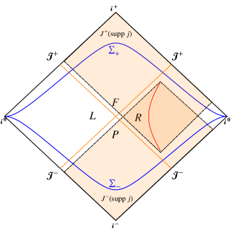
Figure 1: The figure shows the conformal Minkowski spacetime with a uniformly accelerated finite-time source satisfying $z^{2}-t^{2}=1/2$ at the right Rindler wedge $I$. $\Sigma_{\mp}$ represent $t=\mp 2$ past and future Cauchy surfaces of the Minkowski spacetime.

It is important to understand that (for $T\to\infty$) $R=A$ inside the right Rindler wedge B ; RW . In that region the solution is invariant under time reversal and under Rindler time translation. It is not surprising that the temporal Fourier decomposition of such a function involves only the frequency $\omega=0$.

Now, let us analyze the radiation emitted by the scalar source from the perspective of inertial observers in the asymptotic future. For this purpose, we will decompose Eq. (7) in $\Sigma_{+}$ using the so-called Unruh modes U $\left\{w^{1}_{\omega{\bf k}_{\bot}},w^{2}_{\omega{\bf k}_{\bot}}\right\}$, where $\omega\in\mathbb{R}^{+}$ and ${\bf k}_{\perp}\in\mathbb{R}^{2}$. They can be written in terms of left- and right-Rindler modes $v^{R}_{\omega{\bf k}_{\bot}}$ and $v^{L}_{\omega{\bf k}_{\bot}}$, respectively, as

$$w^{1}_{\omega{\bf k}_{\perp}} \equiv \frac{v_{\omega{\bf k}_{\perp}}^{R}+e^{-\pi\omega/a}v_{\omega\,-{\bf k}_{\perp}}^{L*}}{\sqrt{1-e^{-2\pi\omega/a}}},$$ (8)

$$w^{2}_{\omega{\bf k}_{\perp}} \equiv \frac{v_{\omega{\bf k}_{\perp}}^{L}+e^{-\pi\omega/a}v_{\omega\,-{\bf k}_{\perp}}^{R*}}{\sqrt{1-e^{-2\pi\omega/a}}}.$$ (9)

The modes $v_{\omega{\bf k}_{\perp}}^{R}$ vanish in the left Rindler wedge and take the following form in the right Rindler wedge:

$$v_{\omega{\bf k}_{\perp}}^{R}=e^{-i\omega\tau}F_{\omega{\bf k}_{\perp}}(\xi,{\bf x}_{\perp}),$$ (10)

with

$$F_{\omega{\bf k}_{\perp}}(\xi,{\bf x}_{\perp})\equiv\left[\frac{\sinh(\pi\omega/a)}{4\pi^{4}a}\right]^{1/2}K_{i\omega/a}\left(\frac{k_{\perp}}{a}e^{a\xi}\right)e^{i{\bf k}_{\perp}\cdot{\bf x}_{\perp}}.$$ (11)

The modes $v_{\omega{\bf k}_{\perp}}^{L}$ are defined by $v_{\omega{\bf k}_{\perp}}^{L}(t,x,y,z)=v_{\omega{\bf k}_{\perp}}^{R*}(-t,x,y,-z)$. Hence, they vanish in the right Rindler wedge and take the form (10) in Rindler coordinates covering the left Rindler wedge.

The Unruh modes (8) and (9), together with their Hermitian conjugates, form a complete orthonormal set (with respect to the Klein-Gordon inner product CHM08 ) of solutions of the homogeneous Klein-Gordon equation with initial data in certain natural Hilbert spaces. Although they are labeled by Rindler energy $\omega$ and transverse momentum ${\bf k}_{\perp},$ they are positive-frequency with respect to the inertial time $t$. This makes them particularly suitable to analyze the relation between radiation seen by inertial observers and the physics of uniformly accelerated observers. Mathematically, they provide a factorization of the complicated Bogolubov transformation relating the Rindler modes to the conventional modes in Minkowski space: The mapping (Rindler $\leftrightarrow$ Unruh) mixes positive and negative frequency but does not change the spatial dependence of the functions, while the mapping (Unruh $\leftrightarrow$ Minkowski) does not mix the sign of frequency (particles with antiparticles) but interchanges the Rindler eigenfunctions (11) with the conventional plane waves.

Using Eq. (7) and the fact that $\nabla^{a}\nabla_{a}Rj=0$ outside ${\rm supp}\;j$, we can express $Rj$ on $\Sigma_{+}$ in terms of the modes $w^{\sigma}_{\omega{\bf k}_{\perp}}$ ($\sigma=1,2$) as

$$Rj=-\sum_{\sigma=1}^{2}\int_{0}^{\infty}d\omega\int d^{2}{\bf k}_{\perp}\langle w^{\sigma}_{\omega{\bf k}_{\perp}},Ej\rangle_{{}_{\rm KG}}w^{\sigma}_{\omega{\bf k}_{\perp}}+{\rm c.c.},$$ (12)

where $\langle.\;,\;.\rangle_{{}_{\rm KG}}$ denotes the Klein-Gordon inner product. By means of the identity wald90

$$\langle w^{\sigma}_{\omega{\bf k}_{\perp}},Ej\rangle_{{}_{\rm KG}}=i\int_{\mathbb{R}^{4}}d^{4}x\sqrt{-g}{w}^{\sigma*}_{\omega{\bf k}_{\perp}}(x)j(x)$$ (13)

together with Eqs. (3) and (8)-(11), we can compute the expansion coefficients of Eq. (12) as

$$\langle w^{1}_{\omega{\bf k}_{\perp}},Ej\rangle_{{}_{\rm KG}} = \frac{i}{\sqrt{1-e^{-2\pi\omega/a}}}\int_{\mathbb{R}^{4}}d^{4}x\sqrt{-g}{v}^{R{}^{*}}_{\omega{\bf k}_{\perp}}(x)j(x)$$ (14)

$$= \frac{2iq}{\sqrt{1-e^{-2\pi\omega/a}}}\frac{\sin(\omega T)}{\omega}F^{*}_{\omega{\bf k}_{\perp}}(0)$$

and

$$\langle w^{2}_{\omega{\bf k}_{\perp}},Ej\rangle_{{}_{\rm KG}}\!\!\! = \!\!\frac{ie^{-\pi\omega/a}}{\sqrt{1-e^{-2\pi\omega/a}}}\int_{\mathbb{R}^{4}}d^{4}x\sqrt{-g}{v}^{R{}}_{\omega-{\bf k}_{\perp}}(x)j(x)$$ (15)

$$= \frac{2iqe^{-\pi\omega/a}}{\sqrt{1-e^{-2\pi\omega/a}}}\frac{\sin(\omega T)}{\omega}F_{\omega-{\bf k}_{\perp}}(0).$$

Using Eq. (11) in Eqs. (14) and (15) and taking the limit $T\rightarrow\infty$, where the source is uniformly accelerated forever, we obtain

$$\langle w^{1}_{\omega{\bf k}_{\perp}},Ej\rangle_{{}_{\rm KG}}=\langle w^{2}_{\omega{\bf k}_{\perp}},Ej\rangle_{{}_{\rm KG}}=\frac{iqK_{0}(k_{\bot}/a)}{\sqrt{2\pi^{2}a}}\delta(\omega),$$ (16)

where we have used that $\lim_{A\rightarrow\infty}\sin(Ax)/x=\pi\delta(x).$ Now, using Eq. (16) in Eq. (12) together with the fact that $w^{1}_{-\omega{\bf k}_{\bot}}=w^{2}_{\omega{\bf k}_{\bot}}$ CHM08 one obtains

$$Rj=-\frac{iq}{\sqrt{2\pi^{2}a}}\int d^{2}{\bf k}_{\bot}K_{0}(k_{\bot}/a)w^{2}_{0{\bf k}_{\bot}}+c.c.$$ (17)

The above expansion explicitly shows that, in the limit where the charge accelerates forever, only (finite) footnote2 zero-energy Unruh modes contribute to the classical radiation seen by inertial observers in the asymptotic future. We also note that the expansion amplitudes are built entirely from zero-energy Rindler modes in the right wedge [see Eqs. (14)-(16)].

Now, in order to compare our results with the usual results obtained from classical (scalar) electrodynamics, let us explicitly compute the integrals in Eq. (17) when $Rj$ is evaluated in the region $t>|z|$ of Minkowski spacetime. [This “future Rindler wedge” is also associated with the name of Kasner (in dimension 4) or Milne (in dimension 2).] As shown in Ref. CHM08 , the Unruh mode $w^{2}_{\omega{\bf k}_{\bot}}$ can be written as

$$w^{2}_{\omega{\bf k}_{\perp}}=-i\frac{e^{i{\bf k}_{\perp}\cdot{\bf x}_{\perp}+i\omega\zeta}}{\sqrt{32\pi^{2}a}}e^{\pi\omega/2a}H^{(2)}_{i\omega/a}\left(k_{\perp}e^{a\eta}/a\right),$$ (18)

where $H^{(2)}_{\nu}$ is the Hankel function of order $\nu$ and we have introduced the coordinates $\eta,\zeta\in\mathbb{R}$ defined by

$$t=a^{-1}e^{a\eta}\cosh a\zeta,\;z=a^{-1}e^{a\eta}\sinh a\zeta,$$ (19)

which cover the future wedge. By using Eq. (18) in Eq. (17) we can write the retarded solution $Rj$ as

$$Rj=\!\frac{-q}{8\pi^{2}a}\int\!\!d^{2}{\bf k}_{\bot}e^{i{\bf k}_{\perp}\cdot{\bf x}_{\perp}}K_{0}(k_{\bot}/a)H^{(2)}_{0}\left(\frac{k_{\bot}}{a}e^{a\eta}\right)+{\rm c.c.}$$ (20)

In order to compute this integral, let us define polar coordinates $(k_{\perp},\varphi)$ by

$$k_{x}=k_{\perp}\cos\varphi,\>k_{y}=k_{\perp}\sin\varphi.$$

In such coordinates, we can write ${\bf k}_{\perp}\cdot{\bf x}_{\perp}=k_{\perp}x_{\perp}\cos\varphi$, with $x_{\perp}\equiv\sqrt{x^{2}+y^{2}}$, $d^{2}{\bf k}_{\perp}=k_{\perp}d\varphi dk_{\perp}$, and

$$Rj = \frac{-q}{8\pi^{2}a}\int_{0}^{\infty}k_{\perp}dk_{\perp}\int_{0}^{2\pi}d\varphi\left[e^{ik_{\perp}x_{\perp}\cos\varphi}K_{0}(k_{\bot}/a)\right.$$ (21)

$$\left.\times H^{(2)}_{0}\left(\frac{k_{\bot}}{a}e^{a\eta}\right)\right]+{\rm c.c.}$$

We can now perform the integral in $\varphi$ by means of the identity

$$J_{0}(\alpha)=\frac{1}{2\pi}\int_{0}^{2\pi}d\varphi e^{i\alpha\cos\varphi}.$$ (22)

Then, by using $H^{(2)}_{0}\equiv J_{0}-iY_{0}$ we cast Eq. (21) as

$$Rj=\!\frac{-q}{2\pi a}\int_{0}^{\infty}dk_{\perp}k_{\perp}J_{0}(k_{\perp}x_{\perp})K_{0}(k_{\bot}/a)J_{0}\left(k_{\bot}e^{a\eta}/a\right).$$ (23)

Now, by the equality (see Ref. GR or Eq. (132) of Ref. H17 )

$$\int_{0}^{\infty}dk_{\perp}k_{\perp}J_{0}(k_{\perp}x_{\perp})K_{0}(k_{\bot}/a)J_{0}\left(k_{\bot}e^{a\eta}/a\right)=a/2\rho_{0}(x),$$ (24)

where $\rho_{0}(x)\equiv\frac{a}{2}\sqrt{\left(-x^{\mu}x_{\mu}+a^{-2}\right)^{2}+4(t^{2}-z^{2})/a^{2}},$ we find the retarded solution $Rj$ to be

$$Rj=\frac{-q}{4\pi\rho_{0}(x)}.$$ (25)

This is exactly the retarded solution obtained by the usual Green function method of (scalar) electrodynamics (see, for instance, Eq. (2.2) of Ref. RW with $\rho\to-j$).

We stress that the foregoing analysis involves no quantum theory whatsoever. The Rindler and Unruh modes enter only as classical special functions describing the structure of the space of classical solutions of the field equation. Furthermore, no “particle” concept was mentioned and no perturbation theory was employed. Nevertheless, it is possible HM to introduce a notion of “classical particle number” that provides an illuminating comparison with the quantum calculations to follow: Define the classical number of particles radiated (as seen by inertial observers) to be

$$N_{M}\equiv\langle KRj,KRj\rangle_{{}_{\rm KG}},$$ (26)

where

$$KRj\equiv-\frac{iq}{\sqrt{2\pi^{2}a}}\int d^{2}{\bf k}_{\bot}K_{0}(k_{\bot}/a)w^{2}_{0{\bf k}_{\bot}}$$ (27)

is the (inertial-) positive-frequency part of the retarded solution in Eq. (17). Using the orthonormality of the Unruh modes

$$\langle w^{\sigma}_{\omega{\bf k}_{\perp}},w^{\sigma^{\prime}}_{\omega^{\prime}{\bf k^{\prime}}_{\perp}}\rangle_{{}_{\rm KG}}=\delta_{\sigma\sigma^{\prime}}\delta(\omega-\omega^{\prime})\delta({\bf k}_{\bot}-{\bf k^{\prime}}_{\bot}),$$

we substitute Eq. (27) in Eq. (26) to obtain

$$\frac{N_{M}}{T_{\rm tot}} = \frac{q^{2}}{2\pi^{2}a}\int_{0}^{\infty}dk_{\perp}k_{\perp}|K_{0}(k_{\perp}/a)|^{2}$$ (28)

$$= \frac{q^{2}a}{4\pi^{2}},$$

where we have used $T_{\rm tot}=2\pi\delta(\omega)|_{\omega=0}$ and

$$\int_{0}^{\infty}dx\;x|K_{0}(x)|^{2}=1/2.$$

This is exactly the result obtained in RW using tree-level QFT. We will reobtain this result nonperturbatively in the context of QFT in the next section.

III Radiation emitted by an accelerated charge: Quantum aspects

Let us now analyze the radiation emitted by the charge from the point of view of QFT. To unveil the radiation content seen by an inertial observer in the asymptotic future, we now analyze the impact of the source (3) (which is still a c-number and a scalar) on a quantum scalar field $\hat{\phi}$ satisfying

$$\nabla^{a}\nabla_{a}\hat{\phi}=j.$$ (29)

We can write a general solution of this operator equation as

$$\hat{\phi}(t,{\bf x})=Rj(t,{\bf x})\hat{I}+\hat{\phi}_{\rm in}(t,{\bf x}),$$ (30)

where $Rj$ is given by Eq. (6) and $\hat{\phi}_{\rm in}$ satisfies the free (homogeneous) Klein-Gordon equation

$$\nabla^{a}\nabla_{a}\hat{\phi}_{\rm in}=0.$$ (31)

As a result, we can expand $\hat{\phi}_{\rm in}$ as

$$\hat{\phi}_{\rm in}(t,{\bf x})\equiv\sum_{j}\left[u_{j}(t,{\bf x})\hat{a}_{\rm in}({u}^{*}_{j})+{u}^{*}_{j}(t,{\bf x})\hat{a}_{\rm in}^{\dagger}(u_{j})\right],$$ (32)

where $\{u_{j}\}$ is a set of (Minkowski) positive-frequency modes (which might be either plane waves or Unruh modes). Then $|0^{M}_{\rm in}\rangle$ (satisfying $\hat{a}_{\rm in}(u^{*}_{j})|0^{M}_{\rm in}\rangle=0$ for all $j$) is the vacuum state as defined by inertial observers in the asymptotic past, and the Fock space built from the action of $\hat{a}_{\rm in}^{\dagger}(u_{j})$ on $|0^{M}_{\rm in}\rangle$ describes particle states seen by such observers.

Alternatively, we can write a solution of Eq. (29) as

$$\hat{\phi}(t,{\bf x})=Aj(t,{\bf x})\hat{I}+\hat{\phi}_{\rm out}(t,{\bf x}),$$ (33)

where we recall that $Aj$ is the advanced solution of Eq. (5) [which vanishes on $\mathbb{R}^{4}-J^{-}\left({\rm supp}\;j\right)$] and $\hat{\phi}_{\rm out}$ satisfies the free Klein-Gordon equation

$$\nabla^{a}\nabla_{a}\hat{\phi}_{\rm out}=0.$$ (34)

Therefore, the field $\hat{\phi}_{\rm out}$ can be expanded as

$$\hat{\phi}_{\rm out}(t,{\bf x})\equiv\sum_{j}\left[v_{j}(t,{\bf x})\hat{a}_{\rm out}({v}^{*}_{j})+{v}^{*}_{j}(t,{\bf x})\hat{a}_{\rm out}^{\dagger}(v_{j})\right],$$ (35)

where $\{v_{j}\}$ is again a set of (Minkowski) positive-frequency modes (possibly the same as the $u_{j}$). Hence, $|0^{M}_{\rm out}\rangle$ (satisfying $\hat{a}_{\rm out}(v^{*}_{j})|0^{M}_{\rm out}\rangle=0$ for all $j$) is the vacuum state as defined by inertial observers in the asymptotic future and the Fock space built from the action of $\hat{a}_{\rm out}^{\dagger}(v_{j})$ on $|0^{M}_{\rm out}\rangle$ describes particle states seen by such observers.

We can exactly connect the in and out Fock spaces by means of the S-matrix (see, e.g., Sec. 4.1.4 of Ref. IZ ):

$$\hat{S}=\exp{\left[-i\int d^{4}x\sqrt{-g}\;\hat{\phi}_{\rm out}(x)j(x)\right]}.$$ (36)

Let us suppose now that the field is prepared in the in-vacuum, $|0^{M}_{\rm in}\rangle$. Then $\hat{\phi}_{\rm int}$ can be identified with $\hat{\phi}_{\rm out}$, and the S-matrix (36) relates $|0^{M}_{\rm in}\rangle$ and $|0^{M}_{\rm out}\rangle$ as

$$|0^{M}_{\rm in}\rangle=\hat{S}|0^{M}_{\rm out}\rangle.$$ (37)

Next, we use Eq. (37) to analyze how the in-vacuum is seen by inertial observers in the asymptotic future and, as a result, study the radiation emitted by the source. In order to do this, let us first expand $\hat{\phi}_{\rm out}$ in terms of Unruh modes (8) and (9):

$$\hat{\phi}_{\rm out}(x) = \sum_{\sigma=1}^{2}\int_{0}^{\infty}d\omega\int d^{2}{\bf k}_{\perp}\left[w^{\sigma}_{\omega{\bf k}_{\perp}}(x)\hat{a}_{\rm out}(w^{\sigma*}_{\omega{\bf k}_{\perp}})\right.$$ (38)

$$+ \left.w^{\sigma*}_{\omega{\bf k}_{\perp}}(x)\hat{a}_{\rm out}^{\dagger}(w^{\sigma}_{\omega{\bf k}_{\perp}})\right].$$

Now, we smear Eq. (38) with $j$, getting

$$-i\hat{\phi}_{\rm out}(j)\!\!\! \equiv -i\int_{{\mathbb{R}}^{4}}d^{4}x\sqrt{-g}\;\hat{\phi}_{\rm out}(x)j(x)$$ (39)

$$= \!\!\!\sum_{\sigma=1}^{2}\int_{0}^{\infty}\!\!\!\!d\omega\int\!d^{2}{\bf k}_{\perp}\left[\langle w^{\sigma}_{\omega{\bf k}_{\perp}},Ej\rangle^{*}_{{}_{\rm KG}}\hat{a}_{\rm out}(w^{\sigma*}_{\omega{\bf k}_{\perp}})\right.$$

$$- \left.\langle w^{\sigma}_{\omega{\bf k}_{\perp}},Ej\rangle_{{}_{\rm KG}}\hat{a}_{\rm out}^{\dagger}(w^{\sigma}_{\omega{\bf k}_{\perp}})\right],$$

where we have used Eq. (13) to transform the spacetime integral into the Klein-Gordon inner product. The (inertial-) positive-frequency part of $Ej$ is given by

$$KEj\equiv\sum_{\sigma=1}^{2}\int_{0}^{\infty}d\omega\int d^{2}{\bf k}_{\perp}\langle w^{\sigma}_{\omega{\bf k}_{\perp}},Ej\rangle_{{}_{\rm KG}}w^{\sigma}_{\omega{\bf k}_{\perp}},$$ (40)

with which we can rewrite Eq. (39) as

$$i\hat{\phi}_{\rm out}(j)=\hat{a}^{\dagger}_{\rm out}\left(KEj\right)-\hat{a}_{\rm out}\left({KEj}^{*}\right),$$ (41)

where we have used

$$\hat{a}^{\dagger}_{\rm out}\left(KEj\right)\!=\!\sum_{\sigma=1}^{2}\int_{0}^{\infty}\!\!\!d\omega\!\int\!\!d{\bf k}_{\perp}\langle w^{\sigma}_{\omega{\bf k}_{\perp}},Ej\rangle_{{}_{\rm KG}}\hat{a}^{\dagger}_{\rm out}(w^{\sigma}_{\omega{\bf k}_{\perp}})$$ (42)

and analogously for $\hat{a}_{\rm out}\left({KEj}^{*}\right)$. This enables us to cast the S-matrix as

$$\hat{S}=\exp{\left[\hat{a}_{\rm out}\left(KEj^{*}\right)-\hat{a}^{\dagger}_{\rm out}\left(KEj\right)\right]}.$$ (43)

(In Eqs. (41) and (43), ${KEj}^{*}$ is to be read as $(KEj)^{*}$; we prefer not to overload the notation with an extra pair of parentheses.) Applying the Zassenhaus formula,

$$e^{\mathfrak{a}+\mathfrak{b}}=e^{\mathfrak{a}}e^{\mathfrak{b}}e^{-\frac{1}{2}[\mathfrak{a},\mathfrak{b}]}$$

when $[\mathfrak{a},\mathfrak{b}]$ is a c-number, we get from Eqs. (37) and (43) the following expression for the in-vacuum in terms of out-states:

$$|0^{M}_{\rm in}\rangle=e^{-\|KEj\|^{2}/2}e^{-\hat{a}^{\dagger}_{\rm out}\left(KEj\right)}|0^{M}_{\rm out}\rangle,$$ (44)

where

$$\left[\hat{a}_{\rm out}\left(KEj^{*}\right),\hat{a}^{\dagger}_{\rm out}\left(KEj\right)\right] = \langle KEj,KEj\rangle_{{}_{\rm KG}}\hat{I}$$

$$\equiv \|KEj\|^{2}\hat{I}.$$

This is a (multi-mode) coherent state, i.e., it is an eigenstate of $\hat{a}_{\rm out}(w^{\sigma*}_{\omega{\bf k}_{\perp}})$ with eigenvalue $-\langle w^{\sigma}_{\omega{\bf k}_{\perp}},Ej\rangle_{{}_{\rm KG}}$ for all $\sigma\in\{1,2\}$, $\omega\in\mathbb{R}^{+}$, and ${\bf k}_{\perp}\in\mathbb{R}^{2}.$ To see this, we note that

$$\hat{a}_{\rm out}(w^{\sigma*}_{\omega{\bf k}_{\perp}})|0^{M}_{\rm in}\rangle = e^{-\|KEj\|^{2}/2}e^{-\hat{a}^{\dagger}_{\rm out}\left(KEj\right)}\left(e^{\hat{a}^{\dagger}_{\rm out}\left(KEj\right)}\hat{a}_{\rm out}(w^{\sigma*}_{\omega{\bf k}_{\perp}})e^{-\hat{a}^{\dagger}_{\rm out}\left(KEj\right)}\right)|0^{M}_{\rm out}\rangle$$

$$= e^{-\|KEj\|^{2}/2}e^{-\hat{a}^{\dagger}_{\rm out}\left(KEj\right)}\left(\hat{a}_{\rm out}(w^{\sigma*}_{\omega{\bf k}_{\perp}})+\left[\hat{a}^{\dagger}_{\rm out}\left(KEj\right),\hat{a}_{\rm out}(w^{\sigma*}_{\omega{\bf k}_{\perp}})\right]\right)|0^{M}_{\rm out}\rangle$$

where we have used in the second line that

$$e^{\hat{A}}\hat{B}e^{-\hat{A}}=\hat{B}+[\hat{A},\hat{B}]+\frac{1}{2!}[\hat{A},[\hat{A},\hat{B}]]+\cdots.$$ (46)

Using

$$\left[\hat{a}_{\rm out}(w^{\sigma*}_{\omega{\bf k}_{\perp}}),\hat{a}^{\dagger}_{\rm out}\left(KEj\right)\right]=\langle w^{\sigma}_{\omega{\bf k}_{\perp}},KEj\rangle_{{}_{\rm KG}}\hat{I}$$

and $\hat{a}_{\rm out}(w^{\sigma*}_{\omega{\bf k}_{\perp}})|0^{M}_{\rm out}\rangle=0,$ we find that

$$\hat{a}_{\rm out}(w^{\sigma*}_{\omega{\bf k}_{\perp}})|0^{M}_{\rm in}\rangle=-\langle w^{\sigma}_{\omega{\bf k}_{\perp}},Ej\rangle_{{}_{\rm KG}}|0^{M}_{\rm in}\rangle,$$ (47)

where we have also used Eq. (44) and $\langle w^{\sigma}_{\omega{\bf k}_{\perp}},KEj\rangle_{{}_{\rm KG}}=\langle w^{\sigma}_{\omega{\bf k}_{\perp}},Ej\rangle_{{}_{\rm KG}}$.

From Eqs. (38) and (47), it is easy to see that

$$\langle 0^{M}_{\rm in}|\hat{\phi}_{\rm out}|0^{M}_{\rm in}\rangle\!\!\! = \!\!\!-\sum_{\sigma=1}^{2}\int_{0}^{\infty}\!\!\!\!\!d\omega\int\!\!d^{2}{\bf k}_{\perp}\langle w^{\sigma}_{\omega{\bf k}_{\perp}},Ej\rangle_{{}_{\rm KG}}w^{\sigma}_{\omega{\bf k}_{\perp}}$$ (48)

$$+ {\rm c.c.},$$

which is just $-Ej$ written in terms of Unruh modes. By evaluating the above expression on $\Sigma_{+}$, where $Aj=0$, we have that $-Ej=Rj$ and thus (in the far future)

$$\langle 0^{M}_{\rm in}|\hat{\phi}_{\rm out}(x)|0^{M}_{\rm in}\rangle=Rj(x),$$ (49)

which is the classical retarded solution produced by the uniformly accelerated source. Therefore, for such a source interacting with a quantum field $\hat{\phi}$ in the vacuum state defined by inertial observers in the asymptotic past, inertial observers in the asymptotic future will describe this state as a coherent state with field expectation value given by $Rj,$ the classical retarded solution footnote2 .

As we have stressed previously, this solution is built exclusively from zero-energy Rindler modes. Our next task is to show that this property extends not only to the field expectation value but to the quantum state as a whole. Let us delve into the structure of the coherent state (44) to see how each Unruh mode contributes to it in the limit $T_{\rm tot}\rightarrow\infty$. Use Eqs. (14)–(17) to recast Eq. (42) as

$$\!\hat{a}^{\dagger}_{\rm out}\left(KEj\right)=\frac{iq}{\sqrt{2\pi^{2}a}}\int d^{2}{\bf k}_{\bot}K_{0}(k_{\bot}/a)\hat{a}^{\dagger}_{\rm out}\left(w^{2}_{0{\bf k}_{\bot}}\right).$$ (50)

Using Eq. (50) in Eq. (44) one obtains

$$|0_{\rm in}^{M}\rangle=\exp\left[-T_{\rm tot}q^{2}a/(4\pi^{2})\right]$$

$$\bigotimes_{{\bf k}_{\perp}}\exp{\!\!\left[\frac{iqK_{0}({k_{\perp}}/{a})}{\sqrt{2\pi^{2}a}}\hat{a}_{\rm out}^{\dagger}\left(w^{2}_{0{\bf k}_{\bot}}\right)\right]}\!|0_{\rm out}^{M}\rangle,$$ (51)

where we have used that

$$\|KEj\|^{2} = \sum_{\sigma=1}^{2}\int_{0}^{\infty}d\omega\int d^{2}{\bf k}_{\perp}|\langle w^{\sigma}_{\omega{\bf k}_{\perp}}Ej\rangle_{{}_{\rm KG}}|^{2}$$ (52)

$$= q^{2}aT_{\rm tot}/4\pi^{2},$$

which comes from using Eq. (16) in the above equation together with $T_{\rm tot}=2\pi\delta(\omega)|_{\omega=0}$ (as usual in quantum scattering theory). Thus, we see from Eq. (51) that only zero-energy Unruh modes contribute to build the quantum radiation emitted by the charge when the field is initially in the Minkowski vacuum state. This result vindicates the claim that each particle emitted in the inertial frame must correspond in the accelerated one to either the emission or the absorption of a zero-energy Rindler particle HMS92 ,RW .

Let us finish the analysis of the quantum aspects of the radiation by studying both the mean number of created particles and the expectation value of the stress-energy tensor in the asymptotic future. This will allow us to clarify further the connection between the quantum and classical radiation emissions. We begin by using the fact that $|0_{\rm in}^{M}\rangle$ is a coherent state for inertial observers in the asymptotic future — Eq. (47) — to calculate the mean particle number in each Unruh mode:

$$\langle 0_{\rm in}^{M}|\hat{N}^{\rm out}_{\omega{\bf k}_{\perp}}|0_{\rm in}^{M}\rangle = |\langle w^{\sigma}_{\omega{\bf k}_{\perp}},Ej\rangle_{{}_{\rm KG}}|^{2},$$ (53)

where $\hat{N}^{\rm out}_{\omega{\bf k}_{\perp}}=\hat{a}^{\dagger}_{\rm out}(w^{\sigma}_{\omega{\bf k}_{\perp}})\hat{a}_{\rm out}(w^{\sigma*}_{\omega{\bf k}_{\perp}})$ and we have used $\langle 0_{\rm in}^{M}|0_{\rm in}^{M}\rangle=1.$ Integrating over all quantum numbers, we find that the total mean particle number created at the asymptotic future is

$$\langle 0_{\rm in}^{M}|\hat{N}^{\rm out}|0_{\rm in}^{M}\rangle = \sum_{\sigma=1}^{2}\int_{0}^{\infty}d\omega\int d^{2}{\bf k}_{\perp}|\langle w^{\sigma}_{\omega{\bf k}_{\perp}}Ej\rangle_{{}_{\rm KG}}|^{2}.$$

Using Eq. (52) in this equation one obtains

$$\frac{\langle 0_{\rm in}^{M}|\hat{N}^{\rm out}|0_{\rm in}^{M}\rangle}{T_{\rm tot}}=\frac{q^{2}a}{4\pi^{2}},$$ (55)

which agrees with the classical particle number per proper time given in Eq. (28).

Moreover, the agreement between the classical and quantum observables happens not only for the number of emitted scalar particles but also for the (normal-ordered) stress-energy tensor:

$$:\hat{T}^{\rm out}_{ab}:\;\equiv\hat{T}^{\rm out}_{ab}-\langle 0_{\rm out}^{M}|\hat{T}^{\rm out}_{ab}|0_{\rm out}^{M}\rangle,$$ (56)

where $\hat{T}^{\rm out}_{ab}=\nabla_{a}\hat{\phi}_{\rm out}\nabla_{b}\hat{\phi}_{\rm out}-\frac{1}{2}\eta_{ab}\nabla^{c}\hat{\phi}_{\rm out}\nabla_{c}\hat{\phi}_{\rm out}$. To show this, let us use Eqs. (38), (47), and (12) to straightforwardly compute (in the asymptotic future)

$$\langle 0_{\rm in}^{M}|:\nabla_{a}\hat{\phi}_{\rm out}\nabla_{b}\hat{\phi}_{\rm out}:|0_{\rm in}^{M}\rangle=\nabla_{a}Rj\nabla_{b}Rj.$$ (57)

It follows by Eqs. (56)–(57) that on $\mathbb{R}^{4}-J^{-}\left({\rm supp}\;j\right)$ we have

$$\langle 0_{\rm in}^{M}|:\hat{T}^{\rm out}_{ab}:|0_{\rm in}^{M}\rangle\equiv\nabla_{a}Rj\nabla_{b}Rj-\frac{1}{2}\eta_{ab}\nabla^{c}Rj\nabla_{c}Rj,$$

(58)

which is precisely the classical stress-energy tensor associated with the retarded solution, $T_{ab}[Rj]$. As a result, any observable calculated from the expectation value of the quantum stress-energy tensor in the (Minkowski) in-vacuum will be given by its classical counterpart computed from $T_{ab}\left[Rj\right]$. In particular, the (quantum) energy flux integrated along a large sphere in the asymptotic future will be given by RW

$$\int dS^{b}\langle 0_{\rm in}^{M}|:\hat{T}^{\rm out}_{ab}:|0_{\rm in}^{M}\rangle(\partial_{t})^{a}=\frac{q^{2}a^{2}}{12\pi},$$ (59)

which is the usual Larmor formula for the power radiated by a scalar source (with respect to inertial observers). Here, $dS^{b}$ is the vector-valued volume element on the sphere and $(\partial_{t})^{a}$ is the Killing field associated with a global inertial congruence.

IV Conclusions

We have analyzed both classical and quantum aspects of the radiation emitted by a uniformly accelerated scalar source, with emphasis on the limit where the lifetime $T_{\rm tot}$ of the source is infinite. In that case we have shown that the classical radiation is entirely built from zero-energy Unruh modes and that only zero-energy Rindler modes in the right Rindler wedge contribute to the expansion amplitudes. By studying the quantum evolution of the scalar field interacting with a classical uniformly accelerated source, we were able to show how the quantum and classical analyses relate to each other. When the field is prepared in the vacuum state for inertial observers in the asymptotic past, inertial observers in the asymptotic future will describe this state as a coherent multiparticle state whose field expectation value is given by the classical retarded solution $Rj$. This coherent state is built only from zero-energy Unruh modes (agreeing with the classical analysis) and, as in the classical case, only zero-energy Rindler modes in the right Rindler wedge contribute to the amplitudes building the coherent state. It is important to stress that this happens only because the field state is the Minkowski in-vacuum. By computing the mean particle number and the expectation value of the stress-energy tensor in the asymptotic future, we were able to show that they agree with their classical counterparts calculated with the retarded solution. As a result, any (quantum) observables related to the number of particles or stress-energy tensor can be computed using the classical retarded solution. More importantly, zero-energy Rindler modes are not a mathematical artifact; they play a crucial role in building the radiation both in the classical and in the quantum realm. We believe that our results put to rest any doubts questioning the relationship between the Unruh effect and the classical Larmor radiation.

References

(1)
A. Zangwill,
Modern Electrodynamics (Cambridge University Press, Cambridge, 2012).
(2)
J. Larmor,
“On the theory of the magnetic influence on spectra; and on the radiation from moving ions,”
Philosophical Magazine 44, 503 (1897).
(3)
F. Rohrlich,
“The definition of electromagnetic radiation,”
Il Nuovo Cimento 21, 811 (1961).
(4)
F. Rohrlich,
“The principle of equivalence,”
Ann Phys 22, 169 (1963).
(5)
D. G. Boulware,
“Radiation from a uniformly accelerated charge,”
Ann Phys 124, 169 (1980).
(6)
A. Higuchi, G. E. A. Matsas, and D. Sudarsky,
“Bremsstrahlung and zero-energy Rindler photons,”
Phys. Rev. D 45, R3308 (1992).
(7)
A. Higuchi, G. E. A. Matsas, and D. Sudarsky,
“Bremsstrahlung and Fulling–Davies–Unruh thermal bath,”
Phys. Rev. D 46, 3450 (1992).
(8)
A. Higuchi and G. E. A. Matsas,
“Fulling-Davies-Unruh effect in classical field theory,”
Phys. Rev. D 48, 689 (1993).
(9)
H. Ren and E. J. Weinberg,
“Radiation from a moving scalar source,”
Phys. Rev. D 49, 6526 (1994).
(10)
Pauri and Vallisneri,
“Classical roots of the Unruh and Hawking effects,”
Found. Phys. 29, 1499 (1999).
(11)
W. G. Unruh,
“Notes on black hole evaporation,”
Phys. Rev. D 14, 870 (1976).
(12)
G. Cozzella, A. G. S. Landulfo, G. E. A. Matsas, and D. A. T. Vanzella,
“Proposal for observing the Unruh effect with classical electrodynamics,”
Phys. Rev. Lett. 118, 161102 (2017).
(13)
G. Cozzella, A. G. S. Landulfo, G. E. A. Matsas, and D. A. T. Vanzella,
“Quest for a ‘direct’ observation of the Unruh effect with classical electrodynamics:
In honor of Atsushi Higuchi 60th anniversary,”
Int. J. Mod. Phys. D 27, 1843008 (2018).
(14) In order to avoid the appearance of divergences in dealing
with finite-time sources, one must implicitly assume that the source is switched
on/off continously. This is not a source of concern here because we take the limit
before radiation rates are evaluated.
(15)
C. Itzykson and J. B. Zuber,
Quantum Field Theory (McGraw–Hill, New York, 1980).
(16)
L. C. B. Crispino, A. Higuchi, and G. E. A. Matsas,
“The Unruh effect and its applications,”
Rev. Mod. Phys. 80, 787 (2008).
(17)
R. M. Wald,
“Vacuum states in space-times with Killing horizons,”
in Quantum Mechanics in Curved Space-Time, NATO Advaced Study Institutes Series,
Vol. B230, eds. J. Audretsch and V. de Sabbata (D. Reidel Publishing Co, Dordrecht, 1990).
(18) We note that are well
defined through the limit .
(19)
I. S. Gradshteyn and I. M. Ryzhik,
Table of Integrals, Series and Products (Academic Press, New York, 1980).
(20)
A. Higuchi, S. Iso, K. Ueda, and K. Yamamoto,
“Entanglement of the vacuum between left, right, future, and past: the origin of entanglement-induced quantum radiation,”
Phys. Rev. D 96, 083531 (2017).
(21)
We note that Eq. (49) is still valid for any compact support source provided that the
in state is in the Minkowski vacuum.