Linear programming bounds for cliques in Paley graphs

Abstract

The Lovász theta number is a semidefinite programming bound on the clique number of (the complement of) a given graph. Given a vertex-transitive graph, every vertex belongs to a maximal clique, and so one can instead apply this semidefinite programming bound to the local graph. In the case of the Paley graph, the local graph is circulant, and so this bound reduces to a linear programming bound, allowing for fast computations. Impressively, the value of this program with Schrijver’s nonnegativity constraint rivals the state-of-the-art closed-form bound recently proved by Hanson and Petridis. We conjecture that this linear programming bound improves on the Hanson–Petridis bound infinitely often, and we derive the dual program to facilitate proving this conjecture.

1 INTRODUCTION

The Paley graph $G_{p}$ is defined for every prime $p\equiv 1~{}(\operatorname{mod}4)$ with vertex set $\mathbf{F}_{p}=\{0,1,\ldots,p-1\}$, the finite field of $p$ elements, and an edge between $x,y\in\mathbf{F}_{p}$ if and only if $x-y\in Q_{p}$, where

$$Q_{p}:=\{x\in\mathbf{F}_{p}:\text{there exists }y\in\mathbf{F}_{p}\text{ such that }x=y^{2}\}$$

is the multiplicative subgroup of quadratic residues modulo $p$. The Paley graphs provide a family of quasi-random graphs (see Chung, Graham and Wilson[1]) with several nice properties (see §13.2 in Bollobas[2]). For instance, the Paley graph $G_{p}$ is a so-called strongly regular graph in which every vertex has $(p-1)/2$ neighbors, every pair of adjacent vertices share $(p-5)/4$ common neighbors, and every pair of non-adjacent vertices share $(p-1)/4$ common neighbors. The Paley graph of order $p$ can be used to construct an optimal packing of lines through the origin of $\mathbf{R}^{(p+1)/2}$, known as the corresponding Paley equiangular tight frame [3, 4, 5], and these packings have received some attention in the context of compressed sensing [6, 7].

For a simple, undirected graph $G=(V,E)$, we say $C\subseteq V$ is a clique if every pair of vertices in $C$ is adjacent, and we define the clique number of $G$, denoted by $\omega(G)$, to be the size of the largest clique in $G$. It is a famously difficult open problem to determine the order of magnitude of $\omega(G_{p})$ as $p\rightarrow\infty$. The best known closed-form bounds that are valid for all primes $p\equiv 1~{}(\operatorname{mod}4)$ are given by

$$(1+o(1))\frac{\log(p)}{\log(4)}\leq\omega(G_{p})\leq\frac{\sqrt{2p-1}+1}{2}.$$ (1)

The lower bound in (1) is due to Cohen [8]. The same lower bound, with a weaker $o(1)$ term, is actually valid for any self-complementary graph. Recall that the Ramsey number $R(s)$ is the least integer such that every graph on at least $R(s)$ vertices contains either a clique of size $s$ or a set of $s$ pairwise non-adjacent vertices. Then for any self-complementary graph $G$ on at least $R(s)$ vertices, it holds that $\omega(G)\geq s$. Together with the classical upper bound of $R(s)\leq\binom{2s-2}{s-1}$ by Erdős and Szekeres [9], it is straightforward to establish the lower bound in (1). The work of Graham and Ringrose [10] on least quadratic non-residues shows that there exists $c>0$ such that $\omega(G_{p})\geq c\log(p)\log\log\log(p)$ for infinitely many primes $p$, and so the lower bound in (1) is not sharp in general.

The upper bound in (1) was proved very recently by Hanson and Petridis [11] using a clever application of Stepanov’s polynomial method. This improved upon the previously best known closed-form upper bounds of $\omega(G_{p})\leq\sqrt{p-4}$, proved by Maistrelli and Penman [12], and $\omega(G_{p})\leq\sqrt{p}-1$, proved to hold for a majority of primes $p\equiv 1~{}(\operatorname{mod}4)$ by Bachoc, Matolcsi and Ruzsa[13]. Numerical data for primes $p<10000$ by Shearer [14] and Exoo [15] suggests that there should be a polylogarithmic upper bound on $\omega(G_{p})$, but it remains an open problem to determine whether there exists $\epsilon>0$ such that $\omega(G_{p})\leq p^{1/2-\epsilon}$ infinitely often.

This open problem bears some significance in the field of compressed sensing. In particular, Tao [16] posed the problem of finding an explicit family $\{\Phi_{n}\}$ of $m\times n$ matrices with $m=m(n)\in[0.01n,0.99n]$ and $n\to\infty$ for which there exists $\alpha\geq 0.51$ such that for every $n$, it holds that

$$0.5\cdot\|x\|_{2}^{2}~{}\leq~{}\|\Phi_{n}x\|_{2}^{2}~{}\leq~{}1.5\cdot\|x\|_{2}^{2}$$

for every $x\in\mathbb{R}^{n}$ with at most $n^{\alpha}$ nonzero entries. Such matrices are known as restricted isometries. Families of restricted isometries are known to exist for every $\alpha<1$ by an application of the probabilistic method, and yet to date, the best known explicit construction [17, 18] takes $\alpha\leq\frac{1}{2}+10^{-23}$. It is conjectured [7] that the Paley equiangular tight frame behaves as a restricted isometry for a larger choice of $\alpha$, but proving this is difficult, as it would imply the existence of $\epsilon>0$ such that $\omega(G_{p})\leq p^{1/2-\epsilon}$ for all sufficiently large $p$. As partial progress along these lines, the authors recently established that the singular values of random subensembles of the Paley equiangular tight frame obey a Kesten–McKay law [19].

The goal of this paper is to describe a promising approach to find new upper bounds on the clique numbers of Paley graphs. In Section 2, we recall a semidefinite programming approach of Lovász [20] that yields bounds on the clique numbers of arbitrary graphs. By passing to an appropriate subgraph of $G_{p}$, we show that this produces numerical bounds on $\omega(G_{p})$ that usually coincide with the Hanson–Petridis bound and sometimes improve upon it. In Section 3, we show how to compute these bounds by linear programming, extending the range in which we are able to produce computational evidence. In Section 4, we derive the relevant dual program and summarize how one might use weak duality to prove a new bound on $\omega(G_{p})$ by constructing appropriate number-theoretic functions; see Proposition 5. We then conclude with suggestions for future work in this direction.

2 SEMIDEFINITE PROGRAMMING BOUNDS

For a graph $G=(V,E)$, its complement $\overline{G}$ is the graph on vertices $V$ with edges $\binom{V}{2}\setminus E$. An isomorphism between graphs $G=(V,E)$ and $G^{\prime}=(V^{\prime},E^{\prime})$ is a bijection $\varphi\colon V\rightarrow V^{\prime}$ such that $E$ contains an edge between $v,w\in E$ if and only if $E^{\prime}$ contains an edge between $\varphi(v),\varphi(w)\in V^{\prime}$, and an automorphism is an isomorphism between $G$ and itself. When $G$ is isomorphic to $\overline{G}$, we say that $G$ is self-complementary. We say $G=(V,E)$ is vertex-transitive if, for every pair of vertices $v,w\in V$, there exists an automorphism $\varphi$ of $G$ with $\varphi(v)=\varphi(w)$.

In the sequel, we label the vertices of every graph $G$ on $n$ vertices by $\mathbf{Z}_{n}=\{0,1,\ldots,n-1\}$ and similarly index the rows and columns of matrices $X\in\mathbf{R}^{n\times n}$ by $\mathbf{Z}_{n}$ with addition considered modulo $n$. The Lovász theta number for a graph $G$ on $n$ vertices is defined by the semidefinite program

$$\vartheta_{\operatorname{L}}(G)\quad:=\quad\operatorname{max}\quad\displaystyle\sum_{j=0}^{n-1}\sum_{k=0}^{n-1}X_{jk}\quad\text{s.t.}\quad\operatorname{Tr}X=1,\quad X_{jk}=0~{}~{}\forall\{j,k\}\in E(G),\quad X\succeq 0.$$

Lovász [20] proved the following.

Proposition 1.

Let $G$ be any graph on $n$ vertices.

• $\omega(G)\leq\vartheta_{\operatorname{L}}(\overline{G})$.

• If $G$ is vertex-transitive, then $\vartheta_{\operatorname{L}}(G)\vartheta_{\operatorname{L}}(\overline{G})=n$.

Proof.

For (i), suppose $C\subseteq\mathbf{Z}_{n}$ is a maximal clique in $G$, consider the indicator function $1_{C}\colon\mathbf{Z}_{n}\rightarrow\{0,1\}$ as a column vector in $\mathbf{R}^{n}$ indexed by $\mathbf{Z}_{n}$, and put $X:=\frac{1}{\omega(G)}1_{C}1_{C}^{T}$. Then $X$ is feasible in the program $\vartheta_{\operatorname{L}}(\overline{G})$. Counting the nonzero entries of $X$ then gives

$$\omega(G)=\sum_{j=0}^{n-1}\sum_{k=0}^{n-1}X_{jk}\leq\vartheta_{\operatorname{L}}(\overline{G}).$$

The proof of (ii) is more involved; see Theorem 8 in Lovász [20]. ∎

As a consequence of Proposition 1, every self-complementary vertex-transitive graph $G$ on $n$ vertices satisfies $\omega(G)\leq\vartheta_{\operatorname{L}}(G)=\sqrt{n}$. This is enough to recover the well-known bound of $\omega(G_{p})\leq\sqrt{p}$. Indeed, to show that $G_{p}$ is self-complementary, fix any nonzero quadratic non-residue $s\in\mathbf{F}_{p}^{*}\setminus Q_{p}$ and consider the bijection $\mu\colon\mathbf{F}_{p}\rightarrow\mathbf{F}_{p}$ defined by $\mu(x):=sx$. Then for all $v,w\in\mathbf{F}_{p}$, we have $v-w\in Q_{p}$ if and only if $\mu(v)-\mu(w)=s(v-w)\not\in Q_{p}$. That is, $\mu$ is an isomorphism between $G_{p}$ and $\overline{G}_{p}$. To show that $G_{p}$ is vertex-transitive, let $a,b\in\mathbf{F}_{p}$ and consider the map $\tau\colon\mathbf{F}_{p}\rightarrow\mathbf{F}_{p}$ defined by $\tau(x):=x-a+b$. Clearly $\tau(a)=b$. To see that $\tau$ is an automorphism of $G_{p}$, it suffices to observe that for any two vertices $v,w\in\mathbf{F}_{p}$, $\tau(v)-\tau(w)=v-w$. Hence, $\omega(G_{p})\leq\vartheta_{\operatorname{L}}(G_{p})=\sqrt{p}$ follows from Proposition 1.

We can improve upon this bound by focusing our attention to the neighborhood of $0$ in $G_{p}$, namely, the set $Q_{p}$ of quadratic residues. Let $L_{p}$ denote the subgraph of $G_{p}$ induced by $Q_{p}$. Since $G_{p}$ is vertex-transitive, there exists a maximal clique of $G_{p}$ containing the vertex $0$. In particular, $\omega(L_{p})=\omega(G_{p})-1$. By Proposition 1(i), we conclude that

$$\omega(G_{p})\leq\vartheta_{\operatorname{L}}(\overline{L}_{p})+1.$$ (2)

For a graph $G$ on $n$ vertices, Schrijver [21] proposed strengthening $\vartheta_{\operatorname{L}}(G)$ to

$$\vartheta_{\operatorname{LS}}(G)\quad:=\quad\operatorname{max}\quad\displaystyle\sum_{j=0}^{n-1}\sum_{k=0}^{n-1}X_{jk}\quad\text{s.t.}\quad\operatorname{Tr}X=1,\quad X_{jk}=0~{}~{}\forall\{j,k\}\in E(G),\quad X\succeq 0,\quad X\geq 0,$$

where $X\geq 0$ denotes entrywise nonnegativity. Clearly $\vartheta_{\operatorname{LS}}(G)\leq\vartheta_{\operatorname{L}}(G)$, and the proof of Proposition 1(i) further establishes establishes $\omega(G)\leq\vartheta_{\operatorname{LS}}(G)$. This strengthening leads to the bound

$$\omega(G_{p})\leq\vartheta_{\operatorname{LS}}(\overline{L}_{p})+1.$$ (3)

To compare the bounds (2) and (3) to the Hanson–Petridis bound (1), we set

$$\operatorname{HP}(p):=\dfrac{\sqrt{2p-1}+1}{2},\qquad\operatorname{L}(p):=\vartheta_{\operatorname{L}}(\overline{L}_{p})+1,\qquad\operatorname{LS}(p):=\vartheta_{\operatorname{LS}}(\overline{L}_{p})+1,$$

and we compare these in the range $p<3000$ in Figure 1 and Table 1. We observe $\lfloor{\operatorname{L}(p)}\rfloor=\lfloor\operatorname{LS}(p)\rfloor=\lfloor\operatorname{HP}(p)\rfloor$ for most primes in this range, providing an equivalent upper bound on $\omega(G_{p})$. Interestingly, $\lfloor\operatorname{LS}(p)\rfloor=\lfloor\operatorname{HP}(p)\rfloor-1$ for 17 values of $p<3000$.

Gvozdenović, Laurent and Vallentin[22] used semidefinite programming to compute several values of $\operatorname{L}(p)$, which in their notation is $N_{+}(\operatorname{TH}(P_{p}))$. For instance, they compute $\operatorname{L}(809)$ in 4.5 hours on a 3GHz processor with 1GB of RAM. They further introduced the so-called block-diagonal hierarchy of semidefinite programs, which allowed them to compute sharper bounds than $\operatorname{L}(p)$ somewhat more efficiently in the range $p\leq 809$. In order to compute numerical values of $\operatorname{L}(p)$ and $\operatorname{LS}(p)$ efficiently, we leverage the symmetry of $L_{p}$ to reformulate both $\vartheta_{\operatorname{L}}(\overline{L}_{p})$ and $\vartheta_{\operatorname{LS}}(\overline{L}_{p})$ as linear programs in the next section. Using this approach on a 3.4GHz processor with 8GB of RAM, we compute $\operatorname{L}(809)$ in under 20 seconds.

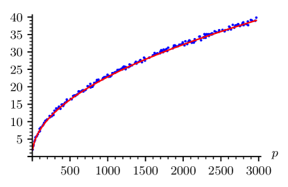
Figure 1: Comparison of $\operatorname{LS}(p)$ and $\operatorname{HP}(p)$ for the 211 primes $p\equiv 1~{}(\operatorname{mod}4)$ with $p<3000$. For 60 such primes, $\operatorname{LS}(p)\leq\operatorname{HP}(p)$. For 17 such primes, $\operatorname{LS}(p)<\lfloor\operatorname{HP}(p)\rfloor$. (left) The blue points $(p,\operatorname{LS}(p))$ appear to concentrate around the red curve $y=\operatorname{HP}(p)$. (right) If a point $(p,\operatorname{LS}(p)-\operatorname{HP}(p))$ lies below the red curve $y=\lfloor\operatorname{HP}(p)\rfloor-\operatorname{HP}(p)$, then $\operatorname{LS}(p)<\lfloor\operatorname{HP}(p)\rfloor$, in which case we plot the point as a circle.

3 REDUCTION TO LINEAR PROGRAMMING

Recall that a matrix $X\in\mathbf{R}^{n\times n}$ is circulant if $X_{j+1,k+1}=X_{jk}$ for all $j,k\in\mathbf{Z}_{n}$. A graph $G$ is said to be circulant if there exists a labeling of its vertices such that its adjacency matrix is circulant. We note that for every prime $p$, the graph $L_{p}$ is circulant. Indeed, select a generator $\alpha$ of the mulitplicative subgroup $Q_{p}$, and order the elements of $Q_{p}$ as $1,\alpha,\ldots,\alpha^{n-1}$. Then $L_{p}$ is circulant since $\alpha^{j}-\alpha^{k}\in Q_{p}$ if and only if $\alpha^{j+1}-\alpha^{k+1}\in Q_{p}$. Since the complement of a circulant graph is also circulant, it holds that $\overline{L}_{p}$ is circulant as well.

Schrijver [21] showed that the semidefinite programming formulations of both $\vartheta_{\operatorname{L}}$ and $\vartheta_{\operatorname{LS}}$ can be reduced to linear programs for certain classes of graphs. In order to state one such linear programming formulation, we take the Fourier transform of $f\colon\mathbf{Z}_{n}\rightarrow\mathbf{C}$ to be the function $\widehat{f}\colon\mathbf{Z}_{n}\rightarrow\mathbf{C}$ defined by

$$\widehat{f}(k):=\sum_{j=0}^{n-1}f(j)e^{-2\pi ijk/n}.$$

Proposition 2.

Let $G$ be any circulant graph with vertex set $\mathbf{Z}_{n}$. Then

$$\vartheta_{\operatorname{L}}(G)\quad=\quad\operatorname{max}\quad n\displaystyle\sum_{k=0}^{n-1}f(k)\quad\text{s.t.}\quad f(0)=\frac{1}{n},\quad f(k)=0~{}~{}\forall\{0,k\}\in E(G),\quad\widehat{f}\geq 0.$$ (4)

Proof.

Let $\vartheta_{\operatorname{LLP}}(G)$ denote the right-hand side of $\eqref{eq:thetaLLP}$. First, we show that $\vartheta_{\operatorname{LLP}}(G)\leq\vartheta_{\operatorname{L}}(G)$. Take any feasible $f$ in the program $\vartheta_{\operatorname{LLP}}(G)$ and consider the circulant matrix $X$ defined by $X_{0k}:=f(k)$. Then $\operatorname{Tr}(X)=1$ follows from $f(0)=1/n$, the edge constraints on $X$ follow from the edge constraints on $f$, and since the eigenvalues of $X$ are the Fourier coefficients $\{\widehat{f}(k):k\in\mathbf{Z}_{n}\}$, we see that $X\succeq 0$ follows from $\widehat{f}\geq 0$. Furthermore, $\sum_{j=0}^{n-1}\sum_{k=0}^{n-1}X_{jk}=n\sum_{k=0}^{n-1}f(k)$. Since every feasible point in $\vartheta_{\operatorname{LLP}}(G)$ can be mapped to a feasible point in $\vartheta_{\operatorname{L}}(G)$ with the same value, we conclude that $\vartheta_{\operatorname{LLP}}(G)\leq\vartheta_{\operatorname{L}}(G)$.

For the other direction, fix any $X^{(0)}$ that is feasible in $\vartheta_{\operatorname{L}}(G)$, and for each $\ell\in\mathbf{Z}_{n}$, consider the matrix $X^{(\ell)}\in\mathbf{R}^{n\times n}$ defined by $X^{(\ell)}_{jk}:=X^{(0)}_{j+\ell,k+\ell}$. Then $X^{(\ell)}$ is also feasible in $\vartheta_{\operatorname{L}}(G)$ with the same value:

$$\sum_{j=0}^{n-1}\sum_{k=0}^{n-1}X^{(\ell)}_{jk}=\sum_{j=0}^{n-1}\sum_{k=0}^{n-1}X^{(0)}_{j+\ell,k+\ell}=\sum_{j=0}^{n-1}\sum_{k=0}^{n-1}X^{(0)}_{jk}.$$

Averaging over this orbit produces a circulant matrix $X:=\frac{1}{n}\sum_{\ell=0}^{n-1}X^{(\ell)}$ that, by convexity, is also feasible in $\vartheta_{\operatorname{L}}(G)$, and that, by linearity, has the same value. Take $f\colon\mathbf{Z}_{n}\rightarrow\mathbf{R}$ defined by $f(k):=X_{0k}$ to obtain a feasible point in $\vartheta_{\operatorname{LLP}}(G)$ with the same value. This implies the reverse inequality $\vartheta_{\operatorname{L}}(G)\leq\vartheta_{\operatorname{LLP}}(G)$. ∎

Arguing similarly establishes the following.

Proposition 3.

Let $G$ be any circulant graph with vertex set $\mathbf{Z}_{n}$. Then

$$\vartheta_{\operatorname{LS}}(G)\quad=\quad\operatorname{max}\quad n\displaystyle\sum_{k=0}^{n-1}f(k)\quad\text{s.t.}\quad f(0)=\frac{1}{n},\quad f(k)=0~{}~{}\forall\{0,k\}\in E(G),\quad\widehat{f}\geq 0,\quad f\geq 0.$$ (5)

We used the linear program formulations in Propositions 2 and 3 to compute the values of $\operatorname{L}(p)$ and $\operatorname{LS}(p)$ reported in Figure 1 and Table 1.

4 DUAL CERTIFICATES

In this section, we derive the dual program of $\vartheta_{\operatorname{LS}}(G)$ for arbitrary circulant graphs $G$. Since every feasible point of the dual program of $\vartheta_{\operatorname{LS}}(\overline{L}_{p})$ gives an upper bound on $\omega(G_{p})$, this section might allow one to prove a new closed-form upper bound on $\omega(G_{p})$. Recall that for a closed convex cone $K\subseteq\mathbf{R}^{n}$, its dual cone is given by

$$K^{*}:=\{y\in\mathbf{R}^{n}:\langle x,y\rangle\geq 0\text{ for all }x\in K\}.$$

Given closed convex cones $K,M\subseteq\mathbf{R}^{n}$, the primal program

$$\operatorname{max}\quad\langle c,x\rangle\quad\text{s.t.}\quad b-Ax\in K,\quad x\in M$$ (6)

has the corresponding dual program

$$\operatorname{min}\quad\langle b,y\rangle\quad\text{s.t.}\quad A^{T}y-c\in M^{*},\quad y\in K^{*}.$$

We will use the above formulation to derive a relatively clean expression for the dual program of (5).

Proposition 4.

Let $G$ be any circulant graph with vertex set $\mathbf{Z}_{n}$. Then

$$\vartheta_{\operatorname{LS}}(G)\quad=\quad\operatorname{min}\quad f(0)\quad\text{s.t.}\quad f(k)=0~{}~{}\forall\{0,k\}\in E(\overline{G}),\quad f\geq g+1,\quad\widehat{g}\geq 0.$$

Proof.

By strong duality, it suffices to show that the right-hand side is the dual program of (5). To this end, we first write the linear program (5) in the form (6). We identify functions $f\colon\mathbf{Z}_{n}\rightarrow\mathbf{R}$ with column vectors in $\mathbf{R}^{n}$ indexed by $\mathbf{Z}_{n}$. Let $P$ denote the projection operator defined by

$$(Pf)(k):=\left\{\begin{array}[]{cl}0&\text{if }\{0,k\}\in E(\overline{G})\\ f(k)&\text{otherwise.}\end{array}\right.$$

Then $f(0)=\frac{1}{n}$ and $f(k)=0$ for every $\{0,k\}\in E(G)$ if and only if $Pf=\frac{1}{n}\delta_{0}$. Next, let $R$ denote the reversal operator defined by $(Rf)(k):=f(-k)$, and let $C$ denote the cosine transform defined by

$$(Cf)(k):=\sum_{j=0}^{n-1}f(j)\cos(2\pi jk/n).$$

Then $f\in\mathbf{R}^{n}$ satisfies $\widehat{f}\geq 0$ if and only if $Rf=f$ and $Cf\geq 0$. Overall, (5) is equivalent to

$$\vartheta_{\operatorname{LS}}(G)\quad=\quad\operatorname{max}\quad\langle n\mathbf{1},f\rangle\quad\text{s.t.}\quad\left[\begin{array}[]{c}\frac{1}{n}\delta_{0}\\ 0\\ 0\end{array}\right]-\left[\begin{array}[]{c}P\\ I-R\\ -C\end{array}\right]f\in\{0\in\mathbf{R}^{n}\}\times\{0\in\mathbf{R}^{n}\}\times\mathbf{R}^{n}_{\geq 0},\quad f\in\mathbf{R}_{\geq 0}^{n},$$

where $\mathbf{R}_{\geq 0}$ denotes the set of nonnegative real numbers. Since $(\{0\in\mathbf{R}^{n}\}\times\{0\in\mathbf{R}^{n}\}\times\mathbf{R}^{n}_{\geq 0})^{*}=\mathbf{R}^{n}\times\mathbf{R}^{n}\times\mathbf{R}_{\geq 0}^{n}$, the dual program is given by following, written in terms of dual variables $y=(u,v,w)\in(\mathbf{R}^{n})^{3}$:

$$\operatorname{min}\quad\frac{1}{n}u(0)\quad\text{s.t.}\quad Pu+(I-R)v-Cw-n\mathbf{1}\in\mathbf{R}^{n}_{\geq 0},\quad w\in\mathbf{R}^{n}_{\geq 0}.$$ (7)

Since $G$ is a circulant graph, we see that $\{0,k\}\in E(G)$ precisely when $\{0,-k\}\in E(G)$, and so $RP=PR$. Also, $RC=CR$. We apply these facts to observe that $(u,v,w)$ is feasible in (7) if and only if $(Ru,-v,Rw)$ is feasible in (7), and with the same value. Indeed, $R$ maps $\mathbf{R}^{n}_{\geq 0}$ to itself, and

$$P(Ru)+(I-R)(-v)-C(Rw)-n\mathbf{1}=R(Pu+(I-R)v-Cw-n\mathbf{1}),\qquad\frac{1}{n}(Ru)(0)=\frac{1}{n}u(0).$$

By averaging these two feasible points, we obtain the following equivalent program:

$$\operatorname{min}\quad\frac{1}{n}u(0)\quad\operatorname{s.t.}\quad Ru=u,\quad Rw=w,\quad Pu\geq Cw+n\mathbf{1},\quad w\geq 0.$$ (8)

At this point, we may relax the constraint $Ru=u$ since $Cw+n\mathbf{1}$ is even. Also, $w\in\mathbf{R}^{n}$ satisfies $Rw=w$ if and only if $Cw=\widehat{w}$. Changing variables to $f=\frac{1}{n}Pu$ and $g=\frac{1}{n}\widehat{w}$ then gives the result. ∎

As such, given a circulant graph $G$, any $(f,g)$ that is feasible in the corresponding linear program in Proposition 4 yields an upper bound on $\vartheta_{\operatorname{LS}}(G)$. Recalling (3), we now specialize to the case of Paley graphs:

Proposition 5.

Given a prime $p\equiv 1~{}(\operatorname{mod}4)$, let $\alpha$ denote a generator of the multiplicative group $Q_{p}$ of quadratic residues modulo $p$, and set $n=(p-1)/2$. Suppose that $f,g\colon\mathbf{Z}_{n}\rightarrow\mathbf{R}$ together satisfy

• $f(k)=0$ for every $k\in\mathbf{Z}_{n}$ with $\alpha^{k}-1\in Q_{p}$,

• $f\geq g+1$, and

• $\widehat{g}\geq 0$.

Then $\omega(G_{p})\leq f(0)+1$.

Arguing similarly to Proposition 4 gives a comparable dual program for $\vartheta_{\operatorname{L}}(G)$. In fact, the resulting program corresponds to adding the constraint $f=g+1$ to the program in Proposition 4. Considering the numerical data in Table 1, we expect these bounds to match frequently.

5 FUTURE WORK

In this paper, we used linear programming to find numerical upper bounds on $\omega(G_{p})$ that usually match and sometimes improve on the Hanson–Petridis bound $\lfloor\operatorname{HP}(p)\rfloor$. Our experiments suggest the following.

Conjecture 6.

For infinitely many primes $p\equiv 1~{}(\operatorname{mod}4)$, it holds that $\operatorname{LS}(p)<\lfloor\operatorname{HP}(p)\rfloor$.

With appropriate number-theoretic functions, one might use Proposition 5 to prove 6. This pursuit of “magic functions” bears some resemblance to recent progress in sphere packing; see Cohn [23] for a survey. We note that Gvozdenović, Laurent and Vallentin[22] introduced a semidefinite programming hierarchy that gives numerical bounds on $\omega(G_{p})$ that are sharper than $\operatorname{HP}(p)$ in the range $p\leq 809$. However, these semidefinite programs are still rather slow. For our linear programming computations, we used GLPK within SageMath [24]. We believe that our code could be sped up significantly by incorporating the fast Fourier transform[25], possibly giving new bounds on $\omega(G_{p})$ for significantly larger primes $p$.

Table 1: Comparison of $\omega(G_{p})$ with the upper bounds $\operatorname{HP}(p),\operatorname{L}(p)$ and $\operatorname{LS}(p)$ for the 63 primes $p\equiv 1~{}(\operatorname{mod}4)$ with $p<3000$ and $\lfloor\operatorname{HP}(p)\rfloor~{}\neq~{}\lfloor\operatorname{LS}(p)\rfloor$. For the 148 unlisted primes $p\equiv 1~{}(\operatorname{mod}4)$ with $p<3000$, we observed $\lfloor\operatorname{HP}(p)\rfloor=\lfloor\operatorname{LS}(p)\rfloor$.

$p$	$\omega(G_{p})$	$\operatorname{HP}(p)$	$\operatorname{L}(p)$	$\operatorname{LS}(p)$
61	5	6.0000	5.9009	5.8886
109	6	7.8655	8.0070	8.0018
173	8	9.7871	10.3165	10.2339
281	7	12.3427	11.9023	11.8916
293	8	12.5934	13.1270	13.1145
353	9	13.7759	14.4454	14.3045
373	8	14.1473	13.7229	13.6952
421	9	15.0000	15.0253	14.9892
457	11	15.6079	16.3859	16.3503
541	11	16.9393	17.4222	17.3589
673	11	18.8371	19.0862	19.0251
733	11	19.6377	20.3389	20.1800
757	11	19.9487	20.1284	20.0668
761	11	20.0000	20.0297	19.9851
773	11	20.1532	19.8771	19.8033
797	9	20.4562	20.1191	19.9988
821	12	20.7546	21.3005	21.1115
829	11	20.8531	21.1864	21.0711
877	13	21.4344	22.2406	22.0372
997	13	22.8215	23.5064	23.4550
1009	11	22.9555	23.2465	23.0941
1013	11	23.0000	23.0713	22.8647
1033	11	23.2211	23.0159	22.9210
1093	12	23.8720	24.2033	24.1343
1181	12	24.7951	25.2438	25.1739
1289	15	25.8821	26.4445	26.4064
1373	14	26.6964	27.3171	27.1684
1481	15	27.7075	28.5703	28.3694
1489	13	27.7809	28.3456	28.1480
1597	13	28.7533	29.0803	29.0021
1613	14	28.8945	29.2067	29.1143
1621	13	28.9649	29.8909	29.7006

$p$	$\omega(G_{p})$	$\operatorname{HP}(p)$	$\operatorname{L}(p)$	$\operatorname{LS}(p)$
1697	13	29.6247	30.1311	30.0687
1709	13	29.7276	30.6383	30.5067
1721	13	29.8300	30.2173	30.1523
1801	14	30.5042	31.3490	31.2143
1949	14	31.7130	32.1343	32.0719
1973	13	31.9046	32.3272	32.1354
2017	13	32.2530	31.9977	31.8802
2029	14	32.3473	33.3049	33.0499
2081	14	32.7529	33.5041	33.3159
2089	14	32.8149	33.3957	33.1789
2113	13	33.0000	32.9818	32.6315
2129	13	33.1228	32.8782	32.7089
2141	13	33.2147	32.7483	32.6685
2213	15	33.7603	34.5759	34.3880
2221	15	33.8204	34.5585	34.4287
2281	17	34.2676	35.2916	35.1050
2309	15	34.4743	35.2676	35.0910
2333	14	34.6504	35.1840	35.0862
2357	15	34.8256	35.2750	35.0886
2477	15	35.6888	36.4402	36.2304
2549	15	36.1966	36.0154	35.9006
2609	15	36.6144	37.5661	37.2694
2617	15	36.6697	37.2249	37.0475
2657	15	36.9452	37.9459	37.7595
2677	15	37.0821	37.1579	36.9388
2789	15	37.8397	38.6001	38.3378
2797	15	37.8932	38.5759	38.4791
2837	15	38.1597	38.1846	37.9661
2861	16	38.3186	37.8309	37.6733
2897	15	38.5559	39.4579	39.1647
2909	15	38.6346	39.2540	39.0498