Polymerization induces non-Gaussian diffusion

Abstract

Recent theoretical modeling offers a unified picture for the description of stochastic processes characterized by a crossover from anomalous to normal behavior. This is particularly welcome, as a growing number of experiments suggest the crossover to be a common feature shared by many systems: in some cases the anomalous part of the dynamics amounts to a Brownian yet non-Gaussian diffusion; more generally, both the diffusion exponent and the distribution may deviate from normal behavior in the initial part of the process. Since proposed theories work at a mesoscopic scale invoking the subordination of diffusivities, it is of primary importance to bridge these representations with a more fundamental, “microscopic” description. We argue that the dynamical behavior of macromolecules during simple polymerization processes provide suitable setups in which analytic, numerical, and particle-tracking experiments can be contrasted at such a scope. Specifically, we demonstrate that Brownian yet non-Gaussian diffusion of the center of mass of a polymer is a direct consequence of the polymerization process. Through the kurtosis, we characterize the early-stage non-Gaussian behavior within a phase diagram, and we also put forward an estimation for the crossover time to ordinary Brownian motion.

I Introduction

Diffusion in crowded and complex systems such as biological cells is usually very heterogeneous, and anomalous behavior – where the mean square displacement of tracers varies non linearly with time – is envisaged Metzler and Klafter (2000); Sanabria et al. (2007); Höfling and Franosch (2013). Over the last few years a new class of diffusive processes has been reported, where the mean square displacement is found to grow linearly in time like in standard, Brownian diffusion, but with a corresponding probability density function (PDF) which is strongly non-Gaussian Weeks et al. (2000); Hapca et al. (2008); Wang et al. (2009); Toyota et al. (2011); Wang et al. (2012); Guan et al. (2014); Ghosh et al. (2014); Wang et al. (2014); Stylianidou et al. (2014); Samanta and Chakrabarti (2016); Dutta and Chakrabarti (2016); Metzler (2017); Cherstvy et al. (2018). This behavior, termed Brownian yet non-Gaussian diffusion Wang et al. (2009, 2012), occurs quite robustly in a wide range of systems, including beads diffusing on lipid tubes Wang et al. (2009) or in networks Wang et al. (2009); Toyota et al. (2011), the motion of tracers in colloidal, polymeric or active suspensions Weeks et al. (2000); Kegel and van Blaaderen (2000); Leptos et al. (2009); Xue et al. (2016) and in biological cellsStylianidou et al. (2014); Parry et al. (2014); Munder et al. (2016), as well as the motion of individuals in heterogeneous populations such as nematodes Hapca et al. (2008). Similar effects on the PDF are also observed in the anomalous diffusion Lampo et al. (2017) of labeled messenger RNA molecules in living $E.coli$ and $S.cervisiae$ cells. In the majority of cases, at larger time the form of the PDF crosses over to the normal, Gaussian one. Therefore, such change cannot be simply due to the heterogeneity of the tracers, unless some of their properties vary with time. More plausibly, the anomalous-to-Gaussian transition might be induced by temporal fluctuations of the diffusion coefficient, due to rearrangements of properties of tracers or of the surrounding medium. To mimic such behaviors, models in which the diffusion varies with time by obeying a stochastic equation has been introduced and solved both analytically than numerically. These models are referred in the literature as the “diffusing diffusivity models” Chubynsky and Slater (2014); Chechkin et al. (2017); Jain and Sebastian (2017a, b); Tyagi and Cherayil (2017); Matse et al. (2017); Jain and Sebastian (2018); Sposini et al. (2018a, b); Grebenkov (2019), and it has been shown that for short times they are intimately related to the idea of superstatistics Beck and Cohen (2003). In the latter approach, an ensemble of particles is assumed to be characterized by different diffusion coefficients and it is then described as a mixture of Gaussian PDFs, weighted by the distribution of the diffusivities. As a result, the ensemble dynamics is still Brownian, yet the PDF of particle displacements corresponds to a Gaussian mixture and it is thus not Gaussian anymore.

Although diffusing diffusivity models qualitatively reproduce the experimental observations, they work at a mesoscopic scale and without a visible connection to the underlying molecular processes. It is therefore becoming increasingly relevant to find a strategy that bridges the gap between the paradigm of diffusing diffusivity and the microscopic realm, in order to fully understand this form of anomalous diffusion. In this paper we show how the diffusion of polymers during a polymerization process offers one possible mechanism to realize this connection. It is well known from polymer theory Doi and Edwards (1988) that the motion of the center of mass of a linear chain is Brownian, but with a diffusivity constant which is inversely proportional to $N^{\alpha}$, where $N$ is the number of monomers and $\alpha$ an exponent ranging from $1/2$ (Rouse model) to $2$ (reptation model). During an equilibrated polymerization processes the number $N$ fluctuates in time and its statistics can be obtained through the exact solution of its stationary master equation. By using a continuous approximation for this temporally homogeneous birth-death Markov process Gillespie (1992), it emerges that in the limit of large systems such process converges to an Ornstein-Uhlenbeck, as it is assumed in most of the diffusing diffusivity models Chechkin et al. (2017). The time scale of the Ornstein-Uhlenbeck process is linearly proportional to the volume of the system and this guarantees that the non-Gaussian behavior can be accessible experimentally by tuning such parameter.

II Polymerization process

Polymers are made of relatively simple subunits (monomers) assembled with one another through different mechanisms and geometries. The result is a macromolecule which may contain from a few tens (in the case oligomers), to several thousand monomer units Flory (1942), or even millions as in the case of DNA and RNA molecules. From a biological point of view, the polymerization process occurs regularly either within or outside the cell Paul (2012) . In particular, cells might trigger polymerization by several mechanisms such as the de novo nucleation of new filaments, the uncapping of existing barbed ends (actin) and rescuing a depolymerizing filament (commonly observed for microtubules).

In order to guarantee the existence of equilibrium conditions, here we consider a polymerization process occurring in a closed volume with a fixed total number of monomers $N_{\mathrm{t}}$. For sake of simplicity, in what follows we suppose that one filament only can nucleate and that subunits may bind reversibly onto both ends of the chain. At each end, the addition and deletion of monomers can be represented as Boal (2002)

$$A_{N}+A_{1}\xrightleftharpoons[k_{-}]{k_{+}}A_{N+1}\,,$$ (1)

where $A_{N}$ is the filament with $N$ subunits, and $k_{+}$, $k_{-}$ are the rate constants for association and dissociation, respectively. Hence,

$$N_{\mathrm{t}}=N(t)+M(t)\,,$$ (2)

where $M(t)=c(t)\,V$ is the number of monomeric subunits, $c$ its concentration and $V$ the system volume. The probability of a filament with $n$ monomers at time $t$ given $n_{0}$ units at time $t_{0}$, $P_{N}(n,t|n_{0},t_{0})$ satisfies the (forward) master equation of a temporally homogeneous birth-death Markov process Gillespie (1992):

$$\begin{array}[]{lll}\partial_{t}P_{N}(n,t|n_{0},t_{0})&=&\left[W_{-}(n+1)\,P_{N}(n+1,t|n_{0},t_{0})-W_{+}(n)\,P_{N}(n,t|n_{0},t_{0})\right]\\ &&+\left[W_{+}(n-1)\,P_{N}(n-1,t|n_{0},t_{0})-W_{-}(n)\,P_{N}(n,t|n_{0},t_{0})\right]\end{array}\,,$$ (3)

with stepping functions

$$\begin{array}[]{l}W_{+}(n)=2k_{+}\,c(n)\quad(1\leq n\leq N_{\mathrm{t}})\,,\\ W_{-}(1)=0\,,\quad W_{-}(2)=k_{-}\,,\quad W_{-}(n)=2k_{-}\quad(3\leq n\leq N_{\mathrm{t}})\,,\end{array}$$ (4)

and $c(n)=(N_{\mathrm{t}}-n)/V$. Through these choices, we are assuming with certainty the existence in solution of a filament with at least one monomer. The factor $2$ in $W_{+}$ models a linear polymer which grows at both ends without developing branching; $W_{-}$ is instead concerned with the possible bonds which may break down. Equilibrium is reached under detailed balance $W_{-}(n)=W_{+}(n)$ ($3\leq n\leq N_{\mathrm{t}}$), corresponding to a polymer composed by

$$N_{\mathrm{eq}}=N_{\mathrm{t}}-\frac{k_{-}}{k_{+}}\,V\equiv\lambda\,N_{\mathrm{t}}$$ (5)

monomers, and to a number

$$M_{\mathrm{eq}}=\frac{k_{-}}{k_{+}}\,V\equiv(1-\lambda)\,N_{\mathrm{t}}$$ (6)

of single monomers in solution. We remark that the rate constants $k_{+}$, $k_{-}$ are specific to the polymerization chemical reactions. Given a certain kind of polymer, the average polymer size and the average number of single monomers in solution are thus controlled by the total number of subunits $N_{\mathrm{t}}$ and by the volume of the system $V$, which are quantities easily controlled in experiments. In the following analysis, we find it convenient to replace the volume with the fraction $0<\lambda<1$ of $N_{\mathrm{t}}$ that compose the polymer at equilibrium; clearly, $V=(1-\lambda)\,N_{\mathrm{t}}\,k_{+}/k_{-}$.

As we prove in the Appendix, for any given $N_{\mathrm{t}}$ and independently from $n_{0}$, the stationary solution $P_{N}(n)\equiv\lim_{t\to\infty}P_{N}(n,t|n_{0},t_{0})$ reads

$$\begin{array}[]{lll}P_{N}(1)&=&\displaystyle\dfrac{1}{\mathcal{N}(N_{\mathrm{t}},\lambda)}\;\dfrac{(1-\lambda)\,N_{\mathrm{t}}}{2\,(N_{\mathrm{t}}-1)}\\ &&\\ P_{N}(2)&=&\displaystyle\dfrac{1}{\mathcal{N}(N_{\mathrm{t}},\lambda)}\\ &&\\ P_{N}(n)&=&\displaystyle\dfrac{2}{\mathcal{N}(N_{\mathrm{t}},\lambda)}\;\frac{(N_{\mathrm{t}}-2)!}{\left[(1-\lambda)\,N_{\mathrm{t}}\right]^{N_{\mathrm{t}}-2}}\;\frac{\left[(1-\lambda)\,N_{\mathrm{t}}\right]^{N_{\mathrm{t}}-n}}{(N_{\mathrm{t}}-n)!}\quad(3\leq n\leq N_{\mathrm{t}})\end{array}\,,$$ (7)

with a normalization factor

$$\mathcal{N}(N_{\mathrm{t}},\lambda) = \frac{N_{\mathrm{t}}\,[(11-4\lambda)\,\lambda-9]+2}{2(N_{\mathrm{t}}-1)}$$ (8)

$$+\frac{2\,(N_{\mathrm{t}}-2)!}{\left[(1-\lambda)\,N_{\mathrm{t}}\right]^{N_{\mathrm{t}}-2}}\;\frac{\Gamma(N_{\mathrm{t}}+1,(1-\lambda)\,N_{\mathrm{t}})}{\Gamma(N_{\mathrm{t}}+1)}\;\mathrm{e}^{(1-\lambda)\,N_{\mathrm{t}}}\,,$$

$\Gamma(\cdot,\cdot)$ being the upper incomplete gamma function Abramowitz and Stegun (1965),

$$\Gamma(N_{\mathrm{t}}+1,(1-\lambda)\,N_{\mathrm{t}})\equiv\int_{(1-\lambda)\,N_{\mathrm{t}}}^{\infty}\mathrm{d}t\,t^{N_{\mathrm{t}}}\,\mathrm{e}^{-t}\,,$$ (9)

and $\Gamma(\cdot)$ the Euler gamma function. We may observe that with $(1-\lambda)\,N_{\mathrm{t}}\to 0$ the two Gamma functions in the normalization factor become equal and simplify to $1$; in this limit, probabilities for small $n$ are suppressed. Indeed, in Section IV we show that $P_{N}(n)$ becomes close to a Gaussian for large $\lambda$ and $N_{\mathrm{t}}$. In view of the inverse power-law relation with the diffusion coefficient of the center of mass, it is however the behavior for small $n$ which affects the probability of large diffusivities, triggering in turn strong deviations from ordinary diffusion which are described in the following Section.

III Brownian yet non-Gaussian diffusion of the center of mass

From polymer physics we know that the center of mass $\bm{R}_{G}$ of a macromolecules with $N$ subunits diffuses with a coefficient $D(N)=D_{0}/N^{\alpha}$, $D_{0}$ being a diffusion coefficient specific of the considered subunit. This means

$$\mathrm{d}\bm{R}_{G}(t)=\sqrt{6\,D(N(t))}\,\mathrm{d}\bm{B}(t)\,,$$ (10)

with $\bm{B}(t)$ a (three-dimensional) Wiener process (Brownian motion). Reference values for the exponent $\alpha$ are:

• $\alpha=1/2$ in the Rouse model Doi and Edwards (1988); Weber et al. (2010), where the polymer is composed of $N$ equivalent beads with neither excluded-volume nor hydrodynamic interaction;

• $\alpha=1$ for the Zimm model Ermak and McCammon (1978); Doi and Edwards (1988), where hydrodynamic is taken into account;

• $\alpha=2$ for the reptation model which describes tagged polymer motion in entangled polymer solutions Doi and Edwards (1978, 1988).

In view of the previous analysis, we understand that polymerization confers a random character to $\bm{R}_{G}$, providing a clear microscopic origin to the “diffusing diffusivity” process we are going to detail next.

From Eq. (7) we readily obtain the stationary distribution for the diffusion coefficient of the polymer’s center of mass,

$$P_{D}(D_{n})=\sum_{n^{\prime}=1}^{N_{\mathrm{t}}}P_{N}(n^{\prime})\;\delta_{D_{n},\frac{D_{0}}{n^{\prime\alpha}}}=P_{N}\left(\dfrac{D_{0}^{\alpha}}{D_{n}^{\alpha}}\right)\quad(1\leq n\leq N_{\mathrm{t}},\;D_{n}=D_{0}/n^{\alpha})\,,$$ (11)

and its first moment

$$D_{\mathrm{av}}\equiv\mathbb{E}[D_{n}]=\sum_{n=1}^{N_{\mathrm{t}}}P_{D}(D_{n})\;D_{n}\,.$$ (12)

Imagine now to perform a particle-tracking experiment at constant $N_{\mathrm{t}}$ and $V$ and to monitor the position of $\bm{R}_{G}$ in stationary conditions. At a given initial instant the polymer possesses a size $n$, and thus a diffusion coefficient $D_{n}=D_{0}/n^{\alpha}$ with probability given by Eq. (11). For time smaller than the characteristic decay $\tau$ of the autocorrelation of the process $N(t)$, the experimental PDF amounts then to a Gaussian mixture (also called “superstatistics”) Wang et al. (2009); Chubynsky and Slater (2014); Beck and Cohen (2003) weighted by Eq. (11). In addition, its second moment grows linearly with time as in the ordinary Brownian motion. Such a phenomenon of “Brownian yet non Gaussian diffusion” Wang et al. (2009, 2012) has been recently modeled at a mesoscopic scale in terms of diffusing diffusivity models Chubynsky and Slater (2014); Chechkin et al. (2017); Jain and Sebastian (2017a, b); Tyagi and Cherayil (2017); Matse et al. (2017); Jain and Sebastian (2018); Sposini et al. (2018a, b); Grebenkov (2019). It is only at time larger than $\tau$ that ordinary (Gaussian) Brownian motion is recovered, with a diffusion coefficient $D_{\mathrm{av}}$. Before giving an estimate of $\tau$ for our model (see next Section), we study the early time non-Gaussianity in the full phase diagram $[N_{\mathrm{t}},\lambda]$, together with its dependence on $\alpha$.

The non-Gaussian behavior distinctive of $\bm{R}_{G}(t)$ at time $0\leq t\ll\tau$ can be properly characterized by referring to one of its Cartesian coordinates, say $x$. The PDF of the $x$-displacements takes the form

$$p_{X}(x,t)=\sum_{n=1}^{N_{\mathrm{t}}}P_{N}\left(\dfrac{D_{0}^{\alpha}}{D_{n}^{\alpha}}\right)\frac{\exp\left({-\frac{x^{2}}{4\pi\,D_{n}t}}\right)}{\sqrt{4\pi D_{n}t}}\,.$$ (13)

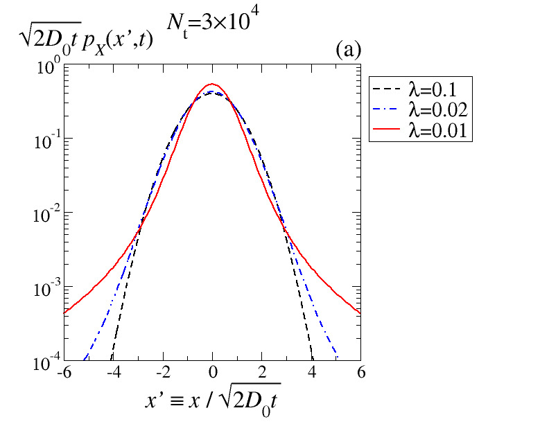
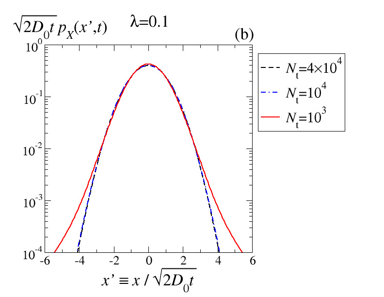
Figure 1: PDF of the $x$-coordinate of $\bm{R}_{G}$ for $0\leq t\ll\tau$, at fixed $N_{\mathrm{t}}$ (a), and fixed $\lambda$ (b). The PDF is rescaled such that the variance is unity; recall that in a log-linear plot Gaussian PDFs have parabolic shape. In both cases, $\alpha=1$.

In Fig. 1 we plot Eq. (13) for $\alpha=1$ and different values of $\lambda$ and $N_{\mathrm{t}}$. At first sight, non-Gaussianity increases with decreasing $N_{\mathrm{t}}$ and and $\lambda$; below we however show that the behavior is not monotonic. To measure deviations from Gaussianity we consider the kurtosis of $p_{X}(x,t)$,

$$\kappa\equiv\frac{\mathbb{E}\left[\left(X-\mathbb{E}[X]\right)^{4}\right]}{\left(\mathbb{E}\left[\left(X-\mathbb{E}[X]\right)^{2}\right]\right)^{2}}\,$$ (14)

($\kappa=3$ for any Gaussian variable). In our case it is straightforward to see that

$$\kappa=3\,\dfrac{\mathbb{E}\left[D^{2}\right]}{\left(\mathbb{E}\left[D\right]\right)^{2}}=3\,\dfrac{\mathbb{E}\left[N^{-2\alpha}\right]}{\left(\mathbb{E}\left[N^{-\alpha}\right]\right)^{2}}\,,$$ (15)

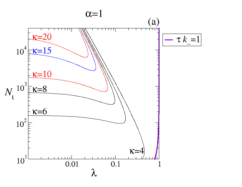
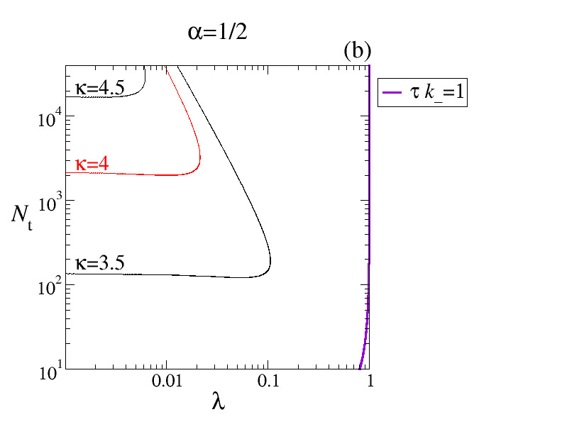
Figure 2: Phase diagram of the early-stage non-Gaussianity. Labeled lines are the kurtosis level curves. The thick, violet line at the right end of the plots corresponds to $\tau\,k_{-}$ (please refer to text for details).

independently of $D_{0}$. Notice instead the strong dependence of $\kappa$ from $\alpha$; moreover, $\kappa>3$ (positive excess kurtosis or leptokurtic PDF). In order to illustrate regions of more pronounced non-Gaussianity and to discuss their dependence on $\alpha$ in Fig. 2 we draw the kurtosis level curves within a $(\lambda,N_{\mathrm{t}})$-phase diagram Note that, for a given pair $(N_{\mathrm{t}},\lambda)$, higher values of the exponent $\alpha$ give rise to larger kurtosis (compare Figs. 2 a and b).

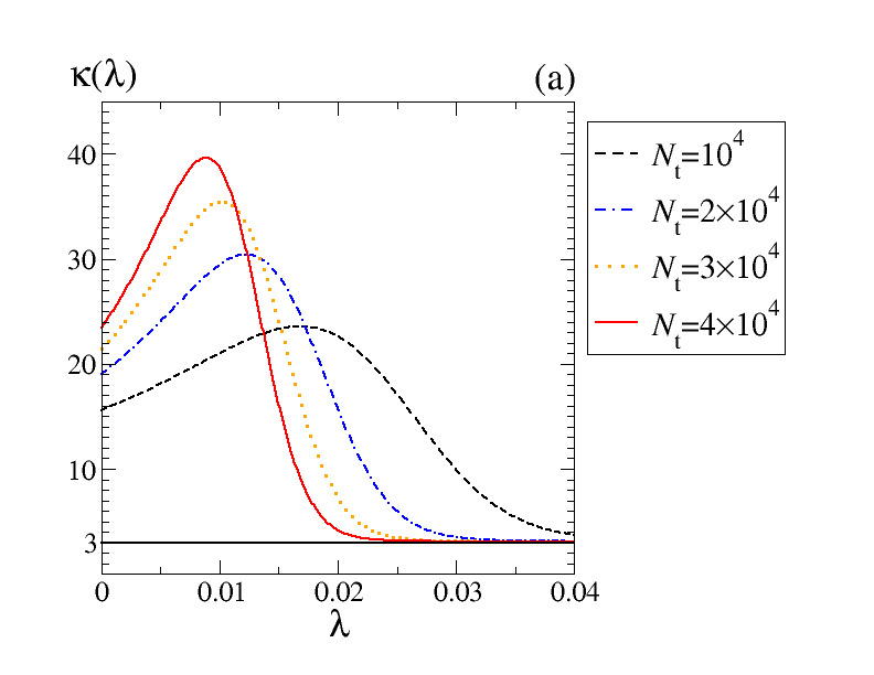
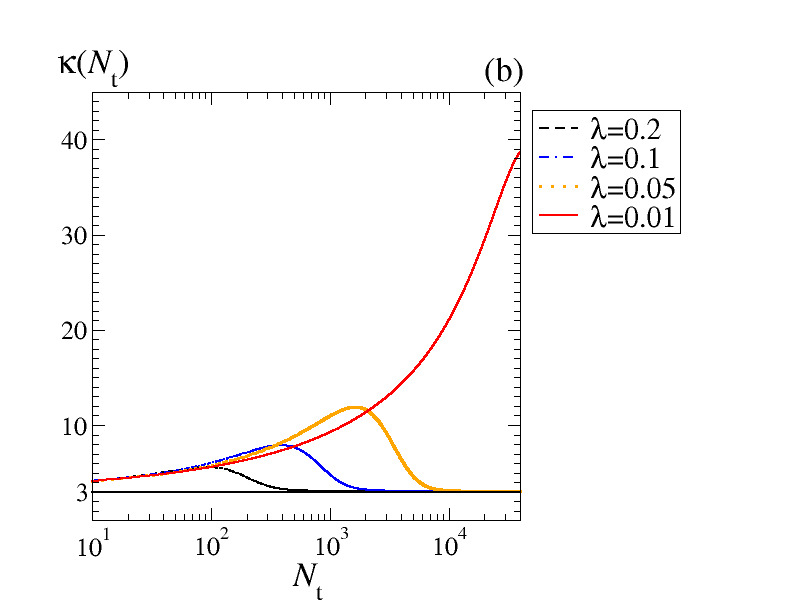
Figure 3: Kurtosis as a function of: (a) $\lambda$; (b) $N_{\mathrm{t}}$. In both cases, $\alpha=1$.

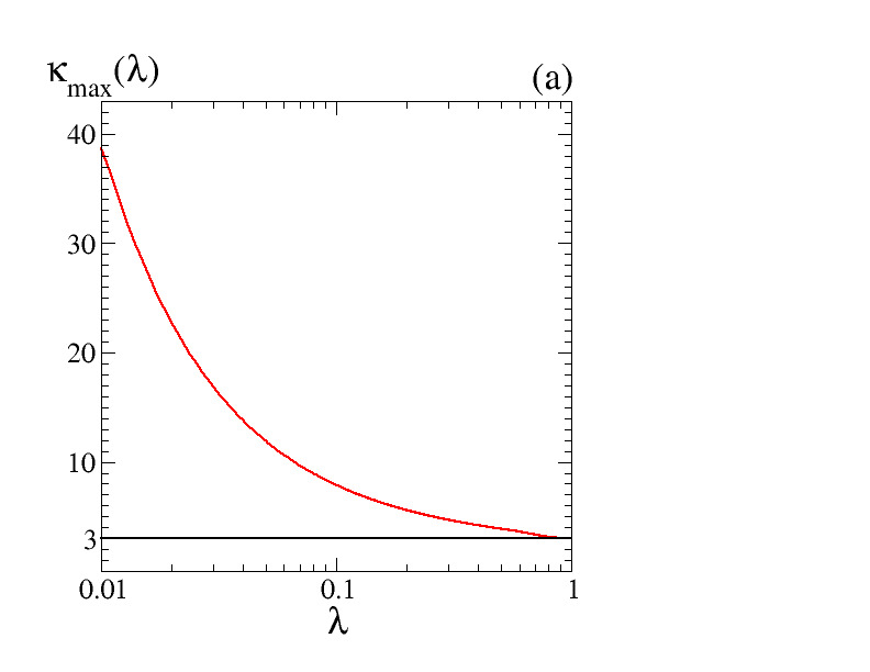
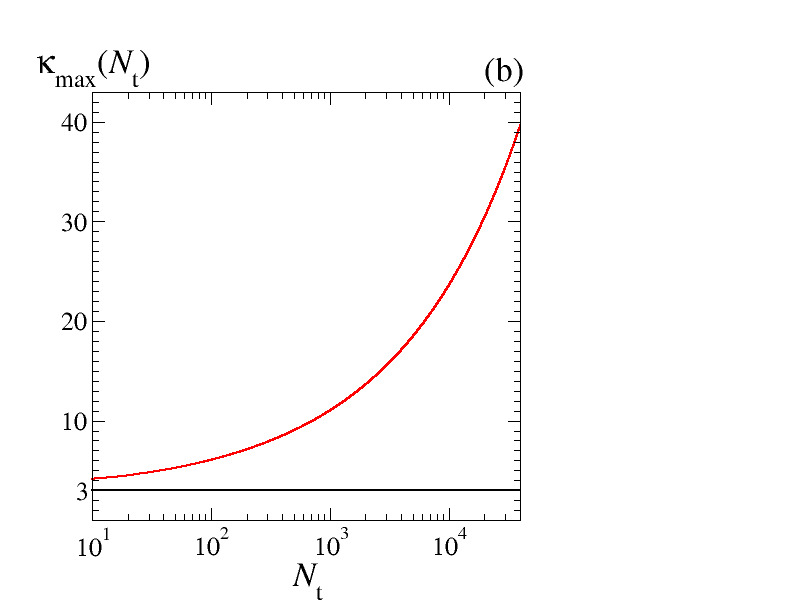
Figure 4: Maximum kurtosis as a function of: (a) $\lambda$; (b) $N_{\mathrm{t}}$. In both cases, $\alpha=1$.

As quoted, by looking at the plots in Fig. 1 one may expect the kurtosis to steadily increase by decreasing $\lambda$ and $N_{\mathrm{t}}$. The structure of the phase diagram implies instead the existence of a maximum kurtosis, both at given $\lambda$ and $N_{\mathrm{t}}$. This is highlighted in Fig. 3. Albeit within a small portion of the phase space, the maximum kurtosis can be extremely high, as reported in Fig. 4; for instance, $k_{\mathrm{max}}\simeq 40$ corresponds to an average polymer size of order $N_{\mathrm{eq}}\simeq 350$ with $N_{\mathrm{t}}\simeq 10^{4}$.

IV Crossover to Brownian, Gaussian diffusion

The stationary distribution in Eq. (7) is exact, but it does not provide information about the decay time-scale $\tau$ of initial conditions for the process $N(t)$. To get such an insight, we next workout a continuous approximation for the polymerization process. In the gedankenexperiment reported above, $\tau$ is the persistence time scale of the randomly chosen initial diffusion coefficient for $\bm{R}_{G}$, corresponding in turn to the typical duration of the leptokurtic PDF for the diffusion of the center of mass.

We start by noticing that around equilibrium, for $N_{\mathrm{t}}\gg 1$ and $N_{\mathrm{eq}}\gg M_{\mathrm{eq}}$ (large $\lambda)$, $N(t)$ can be approximated as a continuous Markov process with Langevin equation Gillespie (1992)

$$\mathrm{d}N(t)=2\frac{k_{+}}{V}\left[N_{\mathrm{eq}}-N(t)\right]\,\mathrm{d}t+\sqrt{2\frac{k_{+}}{V}\left[2N_{\mathrm{t}}-N_{\mathrm{eq}}-N(t)\right]}\,\mathrm{d}B(t)\,,$$ (16)

where $B(t)$ is a Wiener process (Brownian motion). Taking further advantage of the large $N_{\mathrm{eq}}$ assumption, we then introduce the rescaled quantity $\widetilde{N}\equiv N/N_{\mathrm{eq}}$, obeying

$$\mathrm{d}\widetilde{N}(t)=2\frac{k_{+}}{V}\left[1-\widetilde{N}(t)\right]\,\mathrm{d}t+\left(\frac{1}{N_{\mathrm{eq}}}\right)^{1/2}\sqrt{2\frac{k_{+}}{V}\left[2\frac{N_{\mathrm{t}}}{N_{\mathrm{eq}}}-1-\widetilde{N}(t)\right]}\,\mathrm{d}B(t)\,,$$ (17)

to which we may apply the weak noise approximation. Indeed, one may straightforwardly prove Gillespie (1992) that for large $N_{\mathrm{eq}}$ Eq. (17) is satisfied by the approximate solution

$$\widetilde{N}(t)\simeq\widetilde{n}(t)+\left(\frac{1}{N_{\mathrm{eq}}}\right)^{1/2}Y(t)\,,$$ (18)

with $\widetilde{n}(t)$ a deterministic process satisfying

$$\frac{\mathrm{d}\widetilde{n}(t)}{\mathrm{d}t}=2\frac{k_{+}}{V}\left[1-\widetilde{n}(t)\right]\,,$$ (19)

and $Y(t)$ the stochastic process defined by the Langevin equation

$$\mathrm{d}Y(t)=-2\frac{k_{+}}{V}\,Y(t)\,\mathrm{d}t+\sqrt{2\frac{k_{+}}{V}\left[2\frac{N_{\mathrm{t}}}{N_{\mathrm{eq}}}-1-\widetilde{n}(t)\right]}\,\mathrm{d}B(t)\,.$$ (20)

The solution of the deterministic process,

$$\widetilde{n}(t)=1+[\widetilde{n}(0)-1]\,\mathrm{e}^{-\frac{t}{\tau}}\,,$$ (21)

asymptotically tends to $1$ with a characteristic decay time

$$\tau\equiv\frac{V}{2k_{+}}=\frac{(1-\lambda)\,N_{\mathrm{t}}}{2k_{-}}\,\,.$$ (22)

Correspondingly, the long-time behavior of $Y(t)$ is that of an Ornstein-Uhlenbeck process:

$$Y(t\to\infty)=\mathbb{N}\left(0,\frac{N_{\mathrm{t}}}{N_{\mathrm{eq}}}-1\right)\,,$$ (23)

where $\mathbb{N}(\mu,\sigma^{2})$ is a Gaussian variable with mean $\mu$ and variance $\sigma^{2}$. Hence, the stationary solution of $\widetilde{N}$ is

$$\widetilde{N}(t\to\infty)=\mathbb{N}\left(1,\frac{M_{\mathrm{eq}}}{N_{\mathrm{eq}}^{2}}\right)\,.$$ (24)

For the polymer size $N=\widetilde{N}\,N_{\mathrm{eq}}$, this implies

$$N(t\to\infty)=\mathbb{N}\left(N_{\mathrm{eq}},M_{\mathrm{eq}}\right)\,.$$ (25)

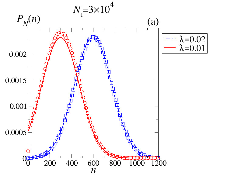
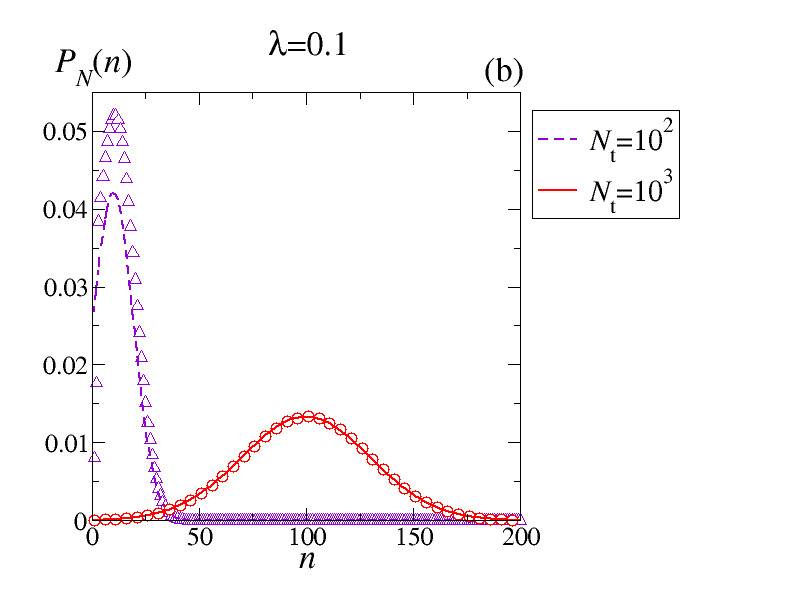
Figure 5: Stationary PDF of the polymerization process. Comparison between the exact PDF in Eq. (7) (symbols) and the continuous, weak noise approximation associated to Eq. (25) (curves). Values for the parameters $N_{\mathrm{t}}$ and $\lambda$ have been chosen to facilitate comparison with Fig. 1. Specifically, continuous red curves correspond to choices in Fig. 1. Decreasing $\lambda$ at fixed $N_{\mathrm{t}}$ (a), or decreasing $N_{\mathrm{t}}$ at fixed $\lambda$ (b) the weak noise approximation breaks down.

We thus appreciate that, to be self consistent, the continuous approximation requires large values of $N_{\mathrm{t}}$ to blur out discreteness, and $N_{\mathrm{eq}}\gg M_{\mathrm{eq}}$ so that the negative support of the Gaussian PDF corresponds to a negligible probability. Fig. 5 shows that when $N_{\mathrm{t}}$ and $\lambda$ are both large the weak noise approximation of the stationary distribution $P_{N}(n)$ is almost indistinguishable from the exact solution. On the other hand, decreasing either $N_{\mathrm{t}}$ or $\lambda$ the approximation fails concomitantly with the fact that the Gaussian probability of negative $n$-values becomes significant. Depending on the specific cut in phase-space, the approximation may or may not work well in correspondence to the maximum kurtosis (compare red full lines in Figs. 5 a and b).

When applicable, the important result conveyed by the continuous, weak noise approximation is that through Eq. (22) it establishes the time scale of the decay of the autocorrelation of $N(t)$. To Fig. 2, we thus added the line

$$\tau\,k_{-}=1\,.$$ (26)

As it depends on the dissociation rate constant specific of the chosen polymer, this line has to be understood qualitatively: according to our estimation, the farther left of the line, the longer lasts the Brownian yet non-Gaussian diffusion stage.

V Conclusions

We have been able to analytically characterize the stochastic motion of the center of mass of a fluctuating filament undergoing a simple polymerization process. Depending on experimentally accessible parameters such as the the total monomers in the solution $N_{\mathrm{t}}$ and the system volume $V$ (equivalently, the fraction $\lambda$ of total monomers composing the filament in equilibrium), the center of mass displays at early times a Brownian, yet non-Gaussian, diffusion. To our knowledge, this is one of the first example in which this anomalous behavior is directly linked to a microscopic prototype: the effect originates from the fluctuations of $N$ (due to polymerization) and from the relation $D(N)=D_{0}/N^{\alpha}$ which distinguishes many microscopic models of polymeric diffusion. By studying the kurtosis of the early-time displacement PDF along the $x$-coordinate we quantified deviations from Gaussian behavior in the phase diagram $(\lambda,N_{\mathrm{t}})$, highlighting the dependence on the exponent $\alpha$. Remarkably, the kurtosis is not monotonic and displays a maximum at either $\lambda$ or $N_{\mathrm{t}}$ fixed. Finally, on the basis of a continuum (weak noise) approximation for the stochastic process $N(t)$, we put forward an estimation for the time $\tau(\lambda,N_{\mathrm{t}})$ at which the anomalous behavior crosses over to ordinary Brownian motion. Since the weak noise approximation is not applicable in the whole $(\lambda,N_{\mathrm{t}})$ phase diagram, and also in view of the non-monotonic behavior of the kurtosis, further studies approaching the determination of $\tau$ are welcome.

In parallel with the analytical results, we proposed a gedankenexperiment in which the anomalous behavior could be detected. As a further perspective, we may notice that if we shift the focus on the diffusion of a tagged monomer (in place of the center of mass of the polymer), in the early stage of the process a subdiffusive behavior coupled to non-Gaussianity is expected to be observed, with a crossover to a Brownian regime at the Rouse time Doi and Edwards (1988). This analysis is intended to be the subject of future work.

In conclusion, we believe that this work provides a valuable analytical backdrop to Brownian yet non-Gaussian diffusion, a fascinating phenomenon reported to occur in many physical systems. To fully understand this anomalous behavior, it is essential to ground it on a microscopic spring. This is the case for the presented model, but we are confident than others more will come along these lines.

Appendix

The stationary distribution $P_{N}(n)\equiv\lim_{t\to\infty}P_{N}(n,t|n_{0},t_{0})$ can be obtained by putting $\partial_{t}P_{N}(n,t|n_{0},t_{0})=0$ in Eq. (3),

$$W_{-}(n+1)\,P_{N}(n+1)=[W_{+}(n)+W_{-}(n)]\,P_{N}(n)-W_{+}(n-1)\,P_{N}(n-1)\,,$$ (27)

and then solving recursively. Let us first consider the case $N=1$. Since with $N_{\mathrm{t}}>0$ we always have at least a polymer of size $1$, $P_{N}(0)=0$. Moreover, as there are no bonds to be broken down with a polymer of size one, $W_{-}(1)=0$. This gives

$$W_{-}(2)\,P_{N}(2)=W_{+}(1)\,P_{N}(1).$$ (28)

With $n=2$, Eq. (27) becomes

$$W_{-}(3)\,P_{N}(3)=[W_{+}(2)+W_{-}(2)]\,P_{N}(2)-W_{+}(1)\,P_{N}(1)$$ (29)

and plugging Eq. (28) into Eq. (29) we get

$$W_{-}(3)\,P_{N}(3)=\frac{W_{+}(2)}{W_{-}(2)}W_{+}(1)\,P_{N}(1).$$ (30)

Since

$$W_{-}(4)\,P_{N}(4)=\frac{W_{+}(3)}{W_{-}(3)}\frac{W_{+}(2)}{W_{-}(2)}W_{+}(1)\,P_{N}(1),.$$ (31)

one can assume for any $n>2$

$$W_{-}(n)\,P_{N}(n)=\left(\prod_{n^{\prime}=2}^{n-1}\frac{W_{+}(n^{\prime})}{W_{-}(n^{\prime}))}\right)W_{+}(1)\,P_{N}(1)\,,$$ (32)

and prove that the same holds with $n+1$. Indeed,

$$W_{-}(n+1)\,P_{N}(n+1) = [W_{+}(n)+W_{-}(n)]\,P_{N}(n)-W_{+}(n-1)\,P_{N}(n-1)$$ (33)

$$= \left[\left(\frac{W_{+}(n)}{W_{-}(n)}+1\right)\left(\prod_{n^{\prime}=2}^{n-1}\frac{W_{+}(n^{\prime})}{W_{-}(n^{\prime})}\right)-\frac{W_{+}(n-1)}{W_{-}(n-1)}\left(\prod_{n^{\prime}=2}^{n-2}\frac{W_{+}(n^{\prime})}{W_{-}(n^{\prime})}\right)\right]W_{+}(1)\,P_{N}(1)$$

$$= \left(\prod_{n^{\prime}=2}^{n}\frac{W_{+}(n^{\prime})}{W_{-}(n^{\prime})}\right)W_{+}(1)\,P_{N}(1)\,.$$

As the normalization condition $\sum_{n=1}^{N_{\mathrm{t}}}P_{N}(n)=1$ gives

$$P_{N}(1)+\frac{W_{+}(1)}{W_{-}(2)}\,P_{N}(1)+\sum_{n=3}^{N_{\mathrm{t}}}\frac{1}{W_{-}(n)}\left(\prod_{n^{\prime}=2}^{n-1}\frac{W_{+}(n^{\prime})}{W_{-}(n^{\prime}))}\right)W_{+}(1)\,P_{N}(1)=1\,,$$ (34)

or

$$W_{+}(1)\,P_{N}(1)=\frac{1}{\frac{1}{W_{+}(1)}+\frac{1}{W_{-}(2)}+\sum_{n=3}^{N_{\mathrm{t}}}\frac{1}{W_{-}(n)}\left(\prod_{n^{\prime}=2}^{n-1}\frac{W_{+}(n^{\prime})}{W_{-}(n^{\prime})}\right)}\,,$$ (35)

we now get

$$\begin{array}[]{lll}P_{N}(1)&=&\displaystyle\frac{\frac{1}{W_{+}(1)}}{\frac{1}{W_{+}(1)}+\frac{1}{W_{-}(2)}+\sum_{n=3}^{N_{\mathrm{t}}}\frac{1}{W_{-}(n)}\left(\prod_{n^{\prime}=2}^{n-1}\frac{W_{+}(n^{\prime})}{W_{-}(n^{\prime})}\right)}\\ &&\\ P_{N}(2)&=&\displaystyle\frac{\frac{1}{W_{-}(2)}}{\frac{1}{W_{+}(1)}+\frac{1}{W_{-}(2)}+\sum_{n=3}^{N_{\mathrm{t}}}\frac{1}{W_{-}(n)}\left(\prod_{n^{\prime}=2}^{n-1}\frac{W_{+}(n^{\prime})}{W_{-}(n^{\prime})}\right)}\\ &&\\ P_{N}(n)&=&\displaystyle\frac{\frac{1}{W_{-}(n)}\;\left(\prod_{n^{\prime}=2}^{n-1}\frac{W_{+}(n^{\prime})}{W_{-}(n^{\prime})}\right)}{\frac{1}{W_{+}(1)}+\frac{1}{W_{-}(2)}+\sum_{n^{\prime}=3}^{N_{\mathrm{t}}}\frac{1}{W_{-}(n^{\prime})}\left(\prod_{n^{\prime\prime}=2}^{n^{\prime}-1}\frac{W_{+}(n^{\prime\prime})}{W_{-}(n^{\prime\prime})}\right)}\quad(3\leq n\leq N_{\mathrm{t}})\end{array}\,.$$ (36)

The result in Eq. (36) is rather general, as the transition rates are not specified. Applying the stepping functions in Eq. (4), we have

$$\begin{array}[]{rll}\dfrac{1}{W_{+}(1)}&=&\dfrac{V}{2k_{+}\,(N_{\mathrm{t}}-1)}=\dfrac{(1-\lambda)\,N_{\mathrm{t}}}{2k_{-}\,(N_{\mathrm{t}}-1)}\\ &&\\ \dfrac{1}{W_{-}(2)}&=&\dfrac{1}{k_{-}}\\ &&\\ \displaystyle\frac{1}{W_{-}(n)}\left(\prod_{n^{\prime}=2}^{n-1}\frac{W_{+}(n^{\prime})}{W_{-}(n^{\prime})}\right)&=&\displaystyle\frac{1}{k_{-}}\;\frac{2k_{+}\,(N_{\mathrm{t}}-2)}{k_{-}\,V}\;\prod_{n^{\prime}=3}^{n-1}\frac{k_{+}\,(N_{\mathrm{t}}-n^{\prime})}{k_{-}\,V}=\frac{2}{k_{-}}\;\left(\frac{k_{+}}{k_{-}\,V}\right)^{n-2}\;\frac{(N_{\mathrm{t}}-2)!}{(N_{\mathrm{t}}-n)!}\\ &&\\ &=&\displaystyle\frac{2}{k_{-}}\;\left[(1-\lambda)\,N_{\mathrm{t}}\right]^{2-n}\;\frac{(N_{\mathrm{t}}-2)!}{(N_{\mathrm{t}}-n)!}\\ &&\\ &=&\displaystyle\frac{2}{k_{-}}\;\frac{(N_{\mathrm{t}}-2)!}{\left[(1-\lambda)\,N_{\mathrm{t}}\right]^{N_{\mathrm{t}}-2}}\;\frac{\left[(1-\lambda)\,N_{\mathrm{t}}\right]^{N_{\mathrm{t}}-n}}{(N_{\mathrm{t}}-n)!}\quad(3\leq n\leq N_{\mathrm{t}})\end{array}\,.$$

Taking advantage of the identity

$$\sum_{n=0}^{N_{{\mathrm{t}}}}\frac{\left[(1-\lambda)\,N_{\mathrm{t}}\right]^{N_{\mathrm{t}}-n}}{(N_{\mathrm{t}}-n)!}=\frac{\Gamma(N_{\mathrm{t}}+1,(1-\lambda)\,N_{\mathrm{t}})}{\Gamma(N_{\mathrm{t}}+1)}\;\mathrm{e}^{(1-\lambda)\,N_{\mathrm{t}}}\,,$$ (37)

$\Gamma(\cdot,\cdot)$ being the upper incomplete gamma function Abramowitz and Stegun (1965), and $\Gamma(\cdot)$ the Euler gamma function, an explicit expression for the normalization factor is

$$\mathcal{N}(N_{\mathrm{t}},\lambda) \equiv \frac{1}{W_{+}(1)}+\frac{1}{W_{-}(2)}+\sum_{n=3}^{N_{\mathrm{t}}}\frac{1}{W_{-}(n)}\left(\prod_{n^{\prime}=2}^{n-1}\frac{W_{+}(n^{\prime})}{W_{-}(n^{\prime})}\right)$$ (39)

$$= \dfrac{(1-\lambda)\,N_{\mathrm{t}}}{2\,(N_{\mathrm{t}}-1)}+1-2\frac{(1-\lambda)^{2}\,N_{\mathrm{t}}}{N_{\mathrm{t}}-1}-2\frac{(1-\lambda)\,N_{\mathrm{t}}}{N_{\mathrm{t}}-1}-2$$

$$+\frac{2\,(N_{\mathrm{t}}-2)!}{\left[(1-\lambda)\,N_{\mathrm{t}}\right]^{N_{\mathrm{t}}-2}}\;\frac{\Gamma(N_{\mathrm{t}}+1,(1-\lambda)\,N_{\mathrm{t}})}{\Gamma(N_{\mathrm{t}}+1)}\;\mathrm{e}^{(1-\lambda)\,N_{\mathrm{t}}}$$

$$= \frac{N_{\mathrm{t}}\,[(11-4\lambda)\,\lambda-9]+2}{2(N_{\mathrm{t}}-1)}$$

$$+\frac{2\,(N_{\mathrm{t}}-2)!}{\left[(1-\lambda)\,N_{\mathrm{t}}\right]^{N_{\mathrm{t}}-2}}\;\frac{\Gamma(N_{\mathrm{t}}+1,(1-\lambda)\,N_{\mathrm{t}})}{\Gamma(N_{\mathrm{t}}+1)}\;\mathrm{e}^{(1-\lambda)\,N_{\mathrm{t}}}\,.$$

Putting things together, the exact stationary solution of Eq. (3) is given by Eq. (7).

Figure captions

Conflict of Interest Statement

The authors declare that the research was conducted in the absence of any commercial or financial relationships that could be construed as a potential conflict of interest.

Author Contributions

All authors equally contributed to the present article.

References

- Metzler and Klafter (2000) R. Metzler and J. Klafter, Physics reports 339, 1 (2000).
- Sanabria et al. (2007) H. Sanabria, Y. Kubota, and M. N. Waxham, Biophysical journal 92, 313 (2007).
- Höfling and Franosch (2013) F. Höfling and T. Franosch, Reports on Progress in Physics 76, 046602 (2013).
- Weeks et al. (2000) E. R. Weeks, J. C. Crocker, A. C. Levitt, A. Schofield, and D. A. Weitz, Science 287, 627 (2000).
- Hapca et al. (2008) S. Hapca, J. W. Crawford, and I. M. Young, Journal of the Royal Society Interface 6, 111 (2008).
- Wang et al. (2009) B. Wang, S. M. Anthony, S. C. Bae, and S. Granick, Proceedings of the National Academy of Sciences 106, 15160 (2009).
- Toyota et al. (2011) T. Toyota, D. A. Head, C. F. Schmidt, and D. Mizuno, Soft Matter 7, 3234 (2011).
- Wang et al. (2012) B. Wang, J. Kuo, S. C. Bae, and S. Granick, Nature materials 11, 481 (2012).
- Guan et al. (2014) J. Guan, B. Wang, and S. Granick, ACS nano 8, 3331 (2014).
- Ghosh et al. (2014) S. K. Ghosh, A. G. Cherstvy, and R. Metzler, The Journal of chemical physics 141, 08B614_1 (2014).
- Wang et al. (2014) D. Wang, R. Hu, M. J. Skaug, and D. K. Schwartz, The journal of physical chemistry letters 6, 54 (2014).
- Stylianidou et al. (2014) S. Stylianidou, N. J. Kuwada, and P. A. Wiggins, Biophysical journal 107, 2684 (2014).
- Samanta and Chakrabarti (2016) N. Samanta and R. Chakrabarti, Soft matter 12, 8554 (2016).
- Dutta and Chakrabarti (2016) S. Dutta and J. Chakrabarti, EPL (Europhysics Letters) 116, 38001 (2016).
- Metzler (2017) R. Metzler, Biophysical journal 112, 413 (2017).
- Cherstvy et al. (2018) A. G. Cherstvy, O. Nagel, C. Beta, and R. Metzler, Physical Chemistry Chemical Physics 20, 23034 (2018).
- Kegel and van Blaaderen (2000) W. K. Kegel and A. van Blaaderen, Science 287, 290 (2000).
- Leptos et al. (2009) K. C. Leptos, J. S. Guasto, J. P. Gollub, A. I. Pesci, and R. E. Goldstein, Physical Review Letters 103, 198103 (2009).
- Xue et al. (2016) C. Xue, X. Zheng, K. Chen, Y. Tian, and G. Hu, The journal of physical chemistry letters 7, 514 (2016).
- Parry et al. (2014) B. R. Parry, I. V. Surovtsev, M. T. Cabeen, C. S. O’Hern, E. R. Dufresne, and C. Jacobs-Wagner, Cell 156, 183 (2014).
- Munder et al. (2016) M. C. Munder, D. Midtvedt, T. Franzmann, E. Nüske, O. Otto, M. Herbig, E. Ulbricht, P. Müller, A. Taubenberger, S. Maharana, et al., Elife 5, e09347 (2016).
- Lampo et al. (2017) T. J. Lampo, S. Stylianidou, M. P. Backlund, P. A. Wiggins, and A. J. Spakowitz, Biophysical journal 112, 532 (2017).
- Chubynsky and Slater (2014) M. V. Chubynsky and G. W. Slater, Physical review letters 113, 098302 (2014).
- Chechkin et al. (2017) A. V. Chechkin, F. Seno, R. Metzler, and I. M. Sokolov, Physical Review X 7, 021002 (2017).
- Jain and Sebastian (2017a) R. Jain and K. Sebastian, Journal of Chemical Sciences 129, 929 (2017a).
- Jain and Sebastian (2017b) R. Jain and K. Sebastian, The Journal of chemical physics 146, 214102 (2017b).
- Tyagi and Cherayil (2017) N. Tyagi and B. J. Cherayil, The Journal of Physical Chemistry B 121, 7204 (2017).
- Matse et al. (2017) M. Matse, M. V. Chubynsky, and J. Bechhoefer, Physical Review E 96, 042604 (2017).
- Jain and Sebastian (2018) R. Jain and K. Sebastian, Physical Review E 98, 052138 (2018).
- Sposini et al. (2018a) V. Sposini, A. V. Chechkin, F. Seno, G. Pagnini, and R. Metzler, New Journal of Physics 20, 043044 (2018a).
- Sposini et al. (2018b) V. Sposini, A. Chechkin, and R. Metzler, Journal of Physics A: Mathematical and Theoretical 52, 04LT01 (2018b).
- Grebenkov (2019) D. Grebenkov, Journal of Physics A: Mathematical and Theoretical (2019).
- Beck and Cohen (2003) C. Beck and E. G. Cohen, Physica A: Statistical mechanics and its applications 322, 267 (2003).
- Doi and Edwards (1988) M. Doi and S. F. Edwards, The theory of polymer dynamics, Vol. 73 (oxford university press, 1988).
- Gillespie (1992) D. T. Gillespie, Markov processes : an introduction for physical scientists (Academic Press, San Diego, CA, US, 1992).
- Flory (1942) P. J. Flory, The Journal of chemical physics 10, 51 (1942).
- Paul (2012) R. Paul, Chem. Modell 9, 61 (2012).
- Boal (2002) D. H. Boal, Mechanics of the Cell (Cambridge University Press, Cambridge, UK, 2002).
- Abramowitz and Stegun (1965) M. Abramowitz and I. A. Stegun, Handbook of mathematical functions: with formulas, graphs, and mathematical tables, Vol. 55 (Courier Corporation, 1965).
- Weber et al. (2010) S. C. Weber, A. J. Spakowitz, and J. A. Theriot, Physical review letters 104, 238102 (2010).
- Ermak and McCammon (1978) D. L. Ermak and J. A. McCammon, The Journal of chemical physics 69, 1352 (1978).
- Doi and Edwards (1978) M. Doi and S. Edwards, Journal of the Chemical Society, Faraday Transactions 2: Molecular and Chemical Physics 74, 1789 (1978).