Kingman’s coalescent with erosion

Abstract

Consider the Markov process taking values in the partitions of $\mathds{N}$ such that each pair of blocks merges at rate one, and each integer is eroded, i.e., becomes a singleton block, at rate $d$. This is a special case of exchangeable fragmentation-coalescence process, called Kingman’s coalescent with erosion. We provide a new construction of the stationary distribution of this process as a sample from a standard flow of bridges. This allows us to give a representation of the asymptotic frequencies of this stationary distribution in terms of a sequence of hierarchically independent diffusions. Moreover, we introduce a new process called Kingman’s coalescent with immigration, where pairs of blocks coalesce at rate one, and new blocks of size one immigrate at rate $d$. By coupling Kingman’s coalescents with erosion and with immigration, we are able to show that the size of a block chosen uniformly at random from the stationary distribution of the restriction of Kingman’s coalescent with erosion to $21[2*{1,\dots,n}$ converges to the total progeny of a critical binary branching process.

1 Introduction

1.1 Motivation

In evolutionary biology, speciation refers to the event when two populations from the same species lose the ability to exchange genetic material, e.g. due to the formation of a new geographic barrier or accumulation of genetic incompatibilities. Even if speciation is usually thought of as irreversible, related species can often still exchange genetic material through exceptional hybridization, migration events or sudden collapse of a geographic barrier (Roux et al., 2016). This can lead to the transmission of chunks of DNA between different species, a phenomenon known as introgression, which is currently considered as a major evolutionary force shaping the genomes of groups of related species (Mallet et al., 2016).

Our study of Kingman’s coalescent with erosion was first motivated by the following simple model of speciation incorporating rare migration events, depicted in Figure 1. Consider a set of $N$ monomorphic species, each harboring a genome of $n$ genes indexed by $21[2*{1,\dots,n}$. We model speciation by assuming that the dynamics of the species is described by a Moran model: at rate one for each pair of species $(s_{1},s_{2})$, species $s_{2}$ dies, $s_{1}$ gives birth to a new species, replicates its genome and sends it into the daughter species. We also model introgression by assuming that at rate $d$ for each gene $g\in 21[2*{1,\dots,n}$ and each pair of species $(s_{1},s_{2})$, $g$ is replicated, the new copy of $g$ is sent from $s_{1}$ to $s_{2}$ and replaces its homolog in $s_{2}$. This assumption is justified by the following view in terms of individual migrants. Each time a migrant goes from $s_{1}$ to $s_{2}$, if recombination is sufficiently strong, its genome rapidly gets washed out by that of the resident species due to the frequent backcrosses (crosses between descendants of the migrant and local residents) so that at most one gene among $n$ reaches fixation.

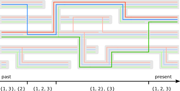
Figure 1: Illustration of the model with $N=5$ species, represented by grey tubes, and $n=3$ genes, represented by the colored lines inside the tubes. A species can split into two, simultaneously replicating its genome (speciation). A gene can replicate and move from one species to another and then replace its homologous copy in the recipient species (introgression). At present time a randomly chosen species is sampled: the ancestral lineages of its genes are represented with bolder colors. The green lineage is first subject to an introgression event and jumps to a new species. It is then brought back to the same species as the other genes by a coalescence event. The corresponding partition-valued process obtained by assigning the labels $1$, $2$ and $3$ to the red, blue and green gene respectively is given.

Now consider a fixed large time $T$, and sample uniformly one species at that time. We follow backwards in time the ancestral lineages of its genes and the ancestral species to which those genes belong. This induces a process valued in the partitions of $21[2*{1,\dots,n}$ by declaring that $i$ and $j$ are in the same block at time $t$ if the ancestral lineages of genes $i$ and $j$ sampled at $T$ lied in the same ancestral species at time $T-t$.

At first ($t=0$), all genes belong to the same ancestral species. Eventually this species receives a successful migrant from another species. Backwards in time, the gene that has been transmitted during this event is removed from its original species and placed in the migrant’s original species. Such events occur at rate $(N-1)d$ for each gene, and the migrant species is then chosen uniformly in the population. Once genes belong to separate species, they can be brought back to the same species by coalescence events. Any two species find their common ancestor at rate one, and at such an event the genes from the two merging species are placed back into the same species.

This informal description shows that the partition-valued process has two kinds of transitions: each pair of blocks merges at rate one; each gene is placed in a new uniformly chosen species at rate $(N-1)d$. Setting the introgression rate to $d_{N}=d/N$ and letting $N\to\infty$, introgression events occur at rate $d$ for each gene. At each such event the gene is sent to a new species that does not contain any of the other $n-1$ ancestral gene lineages, i.e., it is placed in a singleton block. This is the description of Kingman’s coalescent with erosion, that we now more formally introduce.

1.2 Kingman’s coalescent with erosion

Let $n\geq 1$, we define the $n$-Kingman coalescent with erosion as a Markov process $(\Pi^{n}_{t})_{t\geq 0}$ taking values in the partitions of $[n]\coloneqq 21[2*{1,\dots,n}$. Its transition rates are the following. Started from a partition $\pi$ of $[n]$, the process jumps to any partition $\pi^{\prime}$ obtained by merging two blocks of $\pi$ at rate $1$. Moreover, at rate $d$ for each $i\leq n$, the integer $i$ is “eroded”. This means that if $C$ is the block of $\pi$ containing $i$, then the process jumps to the partition $\pi^{\prime}$ obtained by replacing the block $C$ by the blocks $C\mathbin{\mathchoice{\hbox{ \leavevmode\hbox to3.6pt{\vbox to6.6pt{\text{[drawing]}}}}}{\hbox{ \leavevmode\hbox to3.6pt{\vbox to6.6pt{\text{[drawing]}}}}}{\hbox{ \leavevmode\hbox to2.45pt{\vbox to4.45pt{\text{[drawing]}}}}}{\hbox{ \leavevmode\hbox to1.9pt{\vbox to3.4pt{\text{[drawing]}}}}}}21[2*{i}$ and $21[2*{i}$. (Obviously if $C=21[2*{i}$, i.e., if $i$ is in a singleton block, no such transition can occur.)

Kingman’s coalescent with erosion is a special case of the more general class of partition-valued processes called exchangeable fragmentation-coalescence processes, introduced and studied in Berestycki (2004). These processes are a combination of the well-studied fragmentation processes, where blocks can only split, and coalescence processes, where blocks are only allowed to merge. The main new feature of combining fragmentation and coalescence is that they can balance each other so that fragmentation-coalescence processes display non-trivial stationary distributions. In this work we will be interested into describing the stationary distribution associated to Kingman’s coalescent with erosion. The following proposition, which is a direct consequence of Theorem 8 of Berestycki (2004), provides the existence and uniqueness of this distribution.

Proposition 1.1 (Berestycki 2004).

There exists a unique process $(\Pi_{t})_{t\geq 0}$ valued in the partitions of $\mathds{N}$ such that for all $n\geq 1$, the restriction of $(\Pi_{t})_{t\geq 0}$ to $[n]$ is distributed as the $n$-Kingman coalescent with erosion. Moreover, the process $(\Pi_{t})_{t\geq 0}$ has a unique stationary distribution $\Pi$.

Kingman’s coalescent with erosion is an exchangeable process in the sense that for any finite permutation $\sigma$ of $\mathds{N}$,

$$(\sigma(\Pi_{t}))_{t\geq 0}\overset{\mathrm{(d)}}{=}(\Pi_{t})_{t\geq 0}.$$

It is then clear that the stationary distribution $\Pi$ is also an exchangeable partition of $\mathds{N}$. Exchangeable partitions of $\mathds{N}$ are often studied through what is known as their asymptotic frequencies. Let $\Pi=(C_{1},C_{2},\dots)$ be the blocks of the partition $\Pi$. Then, Kingman’s representation theorem (see e.g. Bertoin, 2006) shows that for any $i$, the following limit exists a.s.

$$\lim_{n\to\infty}\frac{1}{n}\sum_{k=1}^{n}\mathds{1}_{\left\{k\in C_{i}\right\}}=f_{i}.$$

Let $(\beta_{i})_{i\geq 1}$ be the non-increasing reordering of the sequence $(f_{i})_{i\geq 1}$. We call $(\beta_{i})_{i\geq 1}$ the asymptotic frequencies of $\Pi$. The sequence $(\beta_{i})_{i\geq 1}$ is such that

$$\beta_{1}\geq\beta_{2}\geq\dots\geq 0,\quad\sum_{i\geq 1}\beta_{i}\leq 1.$$

Such sequences are called mass-partitions. Mass-partitions are studied because exchangeable partitions are entirely characterized by their asymptotic frequencies. The partition $\Pi$ can be recovered from its asymptotic frequencies $(\beta_{i})_{i\geq 1}$ through what is known as a paintbox procedure. Conditionally on $(\beta_{i})_{i\geq 1}$, let $(X_{i})_{i\geq 1}$ be an independent sequence such that for $k\geq 1$, $\mathds{P}_{\!#1}^{#2}\left(X_{i}=k\right)=\beta_{k}$, and $\mathds{P}_{\!#1}^{#2}\left(X_{i}=-i\right)=1-\sum_{k\geq 1}\beta_{k}$. Then the partition $\Pi^{\prime}$ of $\mathds{N}$ defined as

$$i\sim_{\Pi^{\prime}}j\iff X_{i}=X_{j}$$

is distributed as $\Pi$ (see e.g. Bertoin, 2006). We see that $i$ is in a singleton block iff $X_{i}=-i$. The set of all singleton blocks is referred to as the dust of $\Pi$, and the partition $\Pi$ has dust iff $\sum_{i\geq 1}\beta_{i}<1$.

The main characteristics of the asymptotic frequencies of fragmentation-coalescence processes have already been derived in Berestycki (2004), see Theorem 8. In the case of Kingman’s coalescent with erosion, these results specialize to the following theorem.

Theorem 1.2 (Berestycki 2004).

Let $(\beta_{i})_{i\geq 1}$ be the asymptotic frequencies of $\Pi$, the stationary distribution of Kingman’s coalescent with erosion. Then

$$\sum_{i\geq 1}\beta_{i}=1,\quad\forall i\geq 1,\;\beta_{i}>0,\quad a.s.$$

In other words, the partition $\Pi$ has infinitely many blocks, and no dust.

Before stating our main two results, let us motivate them. Consider a partition $\hat{\Pi}$ obtained from a paintbox procedure on a random mass-partition $(\hat{\beta}_{i})_{i\geq 1}$, and denote $\hat{\Pi}^{n}$ its restriction to $[n]$. There are two sources of randomness in $\hat{\Pi}^{n}$. One originates from the fact that $(\hat{\beta}_{i})_{i\geq 1}$ is random. Moreover, conditionally on $(\hat{\beta}_{i})_{i\geq 1}$, $\hat{\Pi}^{n}$ is obtained by sampling a finite number of variables with distribution $(\hat{\beta}_{i})_{i\geq 1}$. Thus, in addition to the randomness of $(\hat{\beta}_{i})_{i\geq 1}$, $\hat{\Pi}^{n}$ is subject to a finite sampling randomness.

Suppose that $\hat{\Pi}$ has finitely many blocks, say $N$, with asymptotic frequencies $(\hat{\beta}_{1},\dots,\hat{\beta}_{N})$. When $n$ gets large, the finite sampling effects vanish and the sizes of the blocks of $\hat{\Pi}^{n}$ resemble $(n\hat{\beta}_{1},\dots,n\hat{\beta}_{N})$. However, when $\hat{\Pi}$ has infinitely many non-singleton blocks, there always exists a large enough $i$ such that the size of the block with frequency $\hat{\beta}_{i}$ remains subject to finite sampling effects in $\hat{\Pi}^{n}$. In this case it is not entirely straightforward to go from the asymptotic frequencies $(\hat{\beta}_{i})_{i\geq 1}$ to the size of the blocks of $\hat{\Pi}^{n}$, as this involves a non-trivial sampling procedure.

In this work our task will be twofold. First, we will investigate the size of the “large blocks” of $\Pi^{n}$ by describing the distribution of the asymptotic frequencies $(\beta_{i})_{i\geq 1}$. In order to get an insight into the distribution of the “small blocks” of $\Pi^{n}$, we will rather study the empirical distribution of the size of the blocks of $\Pi^{n}$, for large $n$. Let us now state the corresponding results.

1.3 Main results

We show two main results in this work. One is concerned with the size of the large blocks of Kingman’s coalescent with erosion, and gives a representation of its asymptotic frequencies in terms of an infinite sequence of hierarchically independent diffusions. The other is concerned with the size of the small blocks and provides the limit of the distribution of the size of a block chosen uniformly from the stationary partition when $n$ is large. Let us start with the former result.

Size of the large blocks.

Let $(Y_{i})_{i\geq 1}$ be an i.i.d. sequence of diffusions verifying

$$\forall i\geq 1,\;\operatorname{\mathrm{d}\!}Y_{i}=(1-Y_{i})\operatorname{\mathrm{d}\!}t+\sqrt{Y_{i}(1-Y_{i})}\operatorname{\mathrm{d}\!}W_{i},$$

started from $0$, and where $(W_{i})_{i\geq 1}$ are independent Brownian motions. It is known, see e.g. Lambert (2008) Proposition 2.3.4, that each $Y_{i}$ is distributed as a Wright-Fisher diffusion conditioned on hitting $1$, and thus we have

$$\forall i\geq 1,\;\lim_{t\to\infty}Y_{i}(t)=1\quad\text{a.s.}$$

Accordingly, we set $Y_{i}(\infty)=1$. We build inductively a sequence of processes $(Z_{i})_{i\geq 1}$ and time-changes $(\tau_{i})_{i\geq 1}$ as follows. Set

$$\forall t\geq 0,\;Z_{1}(t)=Y_{1}(t),\quad\tau_{1}(t)=\int_{0}^{t}\frac{1}{1-Z_{1}(s)}\operatorname{\mathrm{d}\!}s.$$

Then, suppose that $(Z_{1},\dots,Z_{i})$ and $(\tau_{1},\dots,\tau_{i})$ have been defined, and set

$$\forall t\geq 0,\;Z_{i+1}(t)=(1-Z_{1}(t)-\dots-Z_{i}(t))Y_{i+1}(\tau_{i}(t)),$$

$$\forall t\geq 0,\;\tau_{i+1}(t)=\int_{0}^{t}\frac{1}{1-Z_{1}(s)-\dots-Z_{i+1}(s)}\operatorname{\mathrm{d}\!}s.$$

Then we have the following representation of the asymptotic frequencies of the stationary distribution of Kingman’s coalescent with erosion.

Theorem 1.3.

Let $(Z_{i})_{i\geq 1}$ be the sequence of diffusions defined previously. Then the non-increasing reordering of the sequence $(z_{i})_{i\geq 1}$ defined as

$$\forall i\geq 1,\;z_{i}=\int_{0}^{\infty}de^{-dt}Z_{i}(t)\operatorname{\mathrm{d}\!}t,$$

is distributed as the frequencies of the blocks of the stationary distribution of Kingman’s coalescent with erosion rate $d$.

Let us explain the intuition behind Theorem 1.3. Kingman’s coalescent is dual to a measure-valued process called the Fleming-Viot process (Etheridge, 2000). The Fleming-Viot process describes the offspring distribution of a population with constant size, while Kingman’s coalescent gives the genealogy of that population. By a classical duality argument, Kingman’s coalescent at time $t$ can be obtained by sampling individuals at time $t$ from a Fleming-Viot process and placing in the same block those that have the same ancestor (Bertoin and Le Gall, 2003). The link with Theorem 1.3 is that the diffusions $(Z_{i})_{i\geq 1}$ correspond to the sizes of the offspring of the individuals of a Fleming-Viot process, ordered by extinction time of their progeny, see Section 5. The integral transformation is roughly due to the fact that in Kingman’s coalescent with erosion, one needs to place in the same block the individuals that have the same ancestor at their last erosion event, which is an exponential variable with parameter $d$. This heuristical argument is made rigorous in Section 5, where Theorem 1.3 is proved.

Size of the small blocks.

In order to capture the characteristics of the small blocks of $\Pi^{n}$, we study the empirical measure of the size of the blocks of $\Pi^{n}$. Let $M^{n}$ be the total number of blocks of $\Pi^{n}$, and let $(\lvert C^{n}_{1}\rvert,\dots,\lvert C^{n}_{M^{n}}\rvert)$ be their sizes. For each $k\geq 1$, we denote

$$\mu^{n}_{k}=\frac{1}{M^{n}}\operatorname{Card}(21[2*{i\lvert C^{n}_{i}\rvert=k})$$

the frequency of blocks of size $k$. The probability vector $(\mu^{n}_{k})_{k\geq 1}$ is the empirical measure of the size of the blocks of $\Pi^{n}$. We give the following characterization of the asymptotic law of $(\mu^{n}_{k})_{k\geq 1}$ and $M^{n}$.

Theorem 1.4.

1. The following convergence holds in probability

   $$\lim_{n\to\infty}\frac{M^{n}}{\sqrt{n}}=\sqrt{2d}.$$

2. Moreover, for each $k\geq 1$, the following convergence holds in probability

   $$\lim_{n\to\infty}\mu^{n}_{k}=\frac{1}{2^{2k-1}}\frac{1}{k}\binom{2(k-1)}{k-1}=\mathds{P}_{\!#1}^{#2}\left(J=k\right),$$

   where $J$ is the total progeny of a critical binary branching process.

In the previous proposition and hereafter we call critical binary branching process the Markov process on $\mathds{N}$ starting from $1$ that jumps from $k$ to $k+1$ and from $k$ to $k-1$ at rate $k$. Its progeny is the sum of the initial number of particles and of the total number of birth events, i.e., of jumps from $k$ to $k+1$, before the process is absorbed at $0$.

Remark 1.5.

It is interesting to notice that the limiting distribution of the vector $(\mu^{n}_{k})_{k\geq 1}$ is determinisitc and does not depend on the erosion coefficient $d$.

Remark 1.6.

The convergence of the vector $(\mu^{n}_{k})_{k\geq 1}$ is equivalent to the convergence in probability of the empirical measure of the size of the blocks of $\Pi^{n}$ to the distribution of $J$ in the weak topology.

Let us again discuss briefly the heuristic of our proof of this result. Erosion occurs at a rate proportional to the size of the blocks, i.e., a block of size $k$ is eroded at rate $k$, while coalescence events do not take the sizes of the blocks into account. As there are only few blocks with large size in $\Pi^{n}$, and many small blocks, most coalescence events occur between small blocks, while most erosion events occur within these few large blocks. When restricting our attention to small blocks, we can neglect erosion, and consider that pairs of blocks coalesce at rate $1$, and that new blocks of size $1$ appear at constant rate due to the erosion of the large blocks.

This heuristic led us to consider a process analogous to Kingman’s coalescent with erosion, where pairs of blocks coalesce at rate $1$, but new singleton blocks immigrate at constant rate $d$. We call this process Kingman’s coalescent with immigration. We consider the genealogy of a block sampled uniformly from Kingman’s coalescent with immigration. We prove that this genealogy converges, as the immigration rate goes to infinity, to a critical binary birth-death process. See the forthcoming Proposition 3.6.

Outline.

The remainder of the paper is organized as follows. In Section 2 we provide two constructions of Kingman’s coalescent with immigration, as well as a coupling between Kingman’s coalescents with erosion and immigration. Section 3 is then devoted to giving the genealogy of the blocks of Kingman’s coalescent with immigration. We there prove a result analogous to Theorem 1.4, see Proposition 3.1. Theorem 1.4 is proved in Section 4, where we carry out the coupling between Kingman’s coalescents with erosion and immigration. Finally, we prove Theorem 1.3 in Section 5.

Possible extensions.

As we have mentioned, Kingman’s coalescent is part of the more general class of fragmentation-coalescence processes. We now briefly discuss potential extensions of our results to such processes.

The main ingredient of our study of the size of small blocks is that fragmentation is faster for larger blocks, while coalescence occurs at the same speed regardless of the size of the blocks. This allows us to neglect fragmentation and consider a purely coalescing system where new blocks immigrate due to the fragmentation of the large blocks. First, this picture remains valid for $\Lambda$-coalescents with erosion, but the proofs would be more involved because computations could no longer be made explictly. Morever, we believe that this picture also remains valid for a broad class of binary fragmentation measures. The particles that are removed from the large block would no longer be of size one, but should not have time to split on the time-scale when small blocks are formed, yielding a situation similar to the erosion case.

Theorem 1.3 relies on a construction of the stationary distribution of Kingman’s coalescent with erosion from a Fleming-Viot process that can be directly generalized to $\Lambda$-coalescents with erosion (and even to $\Xi$-coalescents with erosion) by using the corresponding $\Lambda$-Fleming-Viot process. However, the explicit expression of the size of the blocks in terms of hierarchically independent diffusions cannot be achieved in general. Nevertheless see the end of Section 5 for a discussion of a possible extension of Theorem 1.3 to Beta-coalescents with erosion.

Overall, the techniques and ideas we use in this work are not entirely specific to Kingman’s coalescent with erosion. Nevertheless, in this case, the proofs are greatly simplified because all calculations can be made explicitly. This reason led us to restrict our attention to Kingman’s coalescent with erosion in this work, and to leave possible extensions for future work.

2 Kingman’s coalescent with immigration

In this section we construct Kingman’s coalescent with immigration as a partition-valued process such that pairs of blocks coalesce at rate $1$ and new blocks immigrate at rate $d$. Then, we give an alternative construction of Kingman’s coalescent with erosion from the flow of bridges of Bertoin and Le Gall (2003). Finally, the coupling between Kingman’s coalescents with erosion and with immigration is carried out in Section 2.4.

2.1 Definition

Consider a Poisson point process on $\mathds{R}$ with intensity $d\operatorname{\mathrm{d}\!}t$, and let $(T_{i})_{i\in\mathds{Z}}$ be its atoms labeled in increasing order such that $T_{0}<0<T_{1}$. The sequence $(T_{i})_{i\in\mathds{Z}}$ corresponds to the immigration times of new particles in the system.

Fix $N\in\mathds{Z}$, we will first define Kingman’s coalescent with immigration for the particles that have a label larger that $N$, and then extend it to all particles by consistency. We do that in the following way. Initially, set

$$\forall t<T_{N},\;\bar{\Pi}^{N}_{t}=\mathchoice{\ooalign{$\displaystyle\mathrm{O}$\cr\raise 1.03334pt\hbox{$\displaystyle\not{}$}\cr}}{\ooalign{$\textstyle\mathrm{O}$\cr\raise 0.94722pt\hbox{$\textstyle\not{}$}\cr}}{\ooalign{$\scriptstyle\mathrm{O}$\cr\raise 0.6458pt\hbox{$\scriptstyle\not{}$}\cr}}{\ooalign{$\scriptscriptstyle\mathrm{O}$\cr\raise 0.38748pt\hbox{$\scriptscriptstyle\not{}$}\cr}}.$$

We now extend $\bar{\Pi}^{N}_{t}$ to all real times by induction. Suppose that $\bar{\Pi}^{N}_{t}$ has been defined on $\left(-\infty,T_{k}\right)$, for $k\geq N$. We first set

$$\bar{\Pi}^{N}_{T_{k}}=\bar{\Pi}^{N}_{T_{k}-}\cup 21[2*{k}$$

to represent the immigration of the new particle with label $k$. We now let each pair of blocks of $\bar{\Pi}^{N}_{t}$ coalesce at rate one for $T_{k}\leq t<T_{k+1}$. One can achieve this by considering, conditional on $21[2*{\bar{\Pi}^{N}_{T_{k}}=\bar{\pi}_{k}}$, an independent version $(\Pi^{k}_{t})_{t\geq 0}$ of Kingman’s coalescent started from $\bar{\pi}_{k}$, and setting

$$\forall t<T_{k+1}-T_{k},\;\bar{\Pi}^{N}_{T_{k}+t}=\Pi^{k}_{t}.$$

We say that the process $(\bar{\Pi}^{N}_{t})_{t\in\mathds{R}}$ is the $N$-Kingman coalescent with immigration rate $d$. The following proposition shows that we can extend consistently the $N$-Kingman’s coalescent with immigration to a process taking its values in the partitions of $\mathds{Z}$, and that it is a Markov process whose transitions coincide with our intuitive description of Kingman’s coalescent with immigration.

Proposition 2.1.

1. There exists a unique process $(\bar{\Pi}_{t})_{t\in\mathds{R}}$, called Kingman’s coalescent with immigration rate $d$, such that for all $N\in\mathds{Z}$, its restriction to $21[2*{i\in\mathds{Z}i\geq N}$ is distributed as the $N$-Kingman coalescent with immigration.

2. With probability one, $\bar{\Pi}_{t}$ has finitely many blocks for all $t\in\mathds{R}$.

3. The process $(\bar{\Pi}_{t})_{t\in\mathds{R}}$ is Markovian. Conditional on $21[2*{\bar{\Pi}_{t}=\bar{\pi}}$, where $\bar{\pi}$ is a partition of $21[2*{i\in\mathds{Z}i\leq n}$, each pair of blocks coalesce at rate $1$, and at rate $d$ the process goes to the partition $\bar{\pi}\cup 21[2*{n+1}$, i.e., a new particle immigrates.

Proof.

(i) Let $(\bar{\Pi}^{N}_{t})_{t\in\mathds{R}}$ be a $N$-Kingman’s coalescent with immigration. It is sufficient to show that the restriction $(\bar{\Pi}^{N+1}_{t})_{t\in\mathds{R}}$ of $(\bar{\Pi}^{N}_{t})_{t\in\mathds{R}}$ to $21[2*{i\in\mathds{Z}i\geq N+1}$ is distributed as a $N+1$-Kingman’s coalescent with immigration, and the result will follow from Kolmogorov’s extension theorem. Obviously, the immigration times of $(\bar{\Pi}^{N+1}_{t})_{t\in\mathds{R}}$ have the desired distribution. The result is now a simple consequence of the sampling consistency of Kingman’s coalescent.

(ii) Let us now prove the second point. Kingman’s coalescent has the property of coming down from infinity (Kingman, 1982). This means that even if Kingman’s coalescent is started from a partition with an infinite number of blocks, then for all positive times it will have only finitely many blocks. Thus, as the number of immigrated particles is locally finite, Kingman’s coalescent with immigration only has a finite number of blocks for all times a.s.

(iii) That each $(\bar{\Pi}^{N}_{t})_{t\in\mathds{R}}$ is a Markov process is a direct consequence of the Markov property of Kingman’s coalescent, and of the fact that the immigration times are distributed according to an independent Poisson point process with intensity $d$. This readily implies the Markov property of $(\bar{\Pi}_{t})_{t\in\mathds{R}}$. ∎

An interesting consequence of the last result is that the process counting the number of blocks of Kingman’s coalescent with immigration is a Markov birth-death process. More precisely, for $t\in\mathds{R}$, let $M_{t}$ be the number of blocks of the partition $\bar{\Pi}_{t}$. Then $(M_{t})_{t\in\mathds{R}}$ is a stationary birth-death process.

Corollary 2.2.

The process $(M_{t})_{t\in\mathds{R}}$ counting the number of blocks of Kingman’s coalescent with immigration rate $d$ is a stationary Markov process. Conditional on $21[2*{M_{t}=k}$, it jumps to

• $k+1$ at rate $d$.

• $k-1$ at rate $k(k-1)/2$.

2.2 Preliminaries on flows of bridges

The previous construction of the Kingman coalescent with immigration is based on Kolmogorov’s extension theorem. The aim of the next two sections is to give an alternative construction of Kingman’s coalescent with immigration based on the flow of bridges of Bertoin and Le Gall (2003). This construction will only be needed in Section 4 for the proof of Theorem 1.3. In this section we recall the material on flows of bridges that will be needed.

Bridges.

We call bridge (Bertoin and Le Gall, 2003) any random function of the form

$$\forall u\in[0,1],\;B(u)=(1-\sum_{i\geq 1}\beta_{i})u+\sum_{i\geq 1}\beta_{i}\mathds{1}_{\left\{u\geq V_{i}\right\}},$$

for some random mass-partition $(\beta_{i})_{i\geq 1}$ and an independent i.i.d. sequence of uniform $[0,1]$ variables $(V_{i})_{i\geq 1}$. For a bridge $B$, we define its inverse $B^{-1}$ as

$$\forall u\in\left[0,1\right),\;B^{-1}(u)=\inf 21[2*{t\in[0,1]B(t)>u},\quad B^{-1}(1)=1.$$

Let $(U_{i})_{i\geq 1}$ be a sequence of i.i.d. uniform variables. An exchangeable partition $\hat{\Pi}$ of $\mathds{N}$ can be obtained from $B$ and $(U_{i})_{i\geq 1}$ by setting

$$i\sim_{\hat{\Pi}}j\iff B^{-1}(U_{i})=B^{-1}(U_{j}).$$

Let $(C_{1},C_{2},\dots)$ be the blocks of $\hat{\Pi}$ labeled in decreasing order of their least elements, i.e., such that

$$i\leq j\iff\min(C_{i})\leq\min(C_{j}).$$

To each block $C_{i}$ is associated a unique random variable $V^{\prime}_{i}$ defined as

$$\forall j\in C_{i},\;V^{\prime}_{i}=B^{-1}(U_{j}).$$

If $\hat{\Pi}$ has finitely many blocks, say $M$, for $i>M$ we set $V^{\prime}_{i}=\tilde{V}^{\prime}_{i}$ where $(\tilde{V}^{\prime}_{i})_{i\geq 1}$ is an independent sequence of i.i.d. uniform random variables. The sequence $(V^{\prime}_{i})_{i\geq 1}$ will be referred to as the sequence of ancestors of the blocks of $\hat{\Pi}$. The key results on bridges from Bertoin and Le Gall (2003) is their Lemma 2 that we state here for later use.

Lemma 2.3 (Bertoin and Le Gall 2003).

Consider a bridge $B$, and let $\hat{\Pi}$ and $(V^{\prime}_{i})$ be respectively the partition and sequence of ancestors obtained from $B$ as above. Then $(V^{\prime}_{i})_{i\geq 1}$ is independent of $\hat{\Pi}$, and $(V^{\prime}_{i})_{i\geq 1}$ is a sequence of i.i.d. uniform variables.

The standard flow of bridges.

A flow of bridges is defined as follows.

Definition 2.4.

A flow of bridges is a family of bridges $(B_{s,t})_{s\leq t}$ such that:

1. For any $s\leq u\leq t$, we have $B_{s,u}\circ B_{u,t}=B_{s,t}$.

2. For $p\geq 1$ and $t_{1}\leq\dots\leq t_{p}$, the bridges $B_{t_{1},t_{2}},\dots,B_{t_{p-1},t_{p}}$ are independent, and $B_{t_{1},t_{2}}$ is distributed as $B_{0,t_{2}-t_{1}}$.

3. The limit $B_{0,t}\to\operatorname{Id}$ as $t\downarrow 0$ holds in probability in the Skorohod space.

A flow of bridges encodes the dynamics of a population represented by the interval $[0,1]$. Let $t\in\mathds{R}$ and $x<y$. If the interval $[x,y]$ is interpreted as a subfamily of the population at time $t$, then its progeny at time $s\leq t$ is represented by the interval $[B_{s,t}(x-),B_{s,t}(y)]$. (Notice that time is going backward: if $t$ is the present, then $s\leq t$ represents the future of the population.)

By the independence and stationarity of the increments of the flow, the distribution of a flow of bridges is entirely characterized by the distribution of $B_{0,t}$, for $t\geq 0$. We will be particularly interested into the so-called standard flow of bridges, that can be described as follows. Let $t\geq 0$ and consider the bridge

$$\forall u\in[0,1],\;B_{0,t}(u)=\sum_{i=1}^{N_{t}}\beta_{i}\mathds{1}_{\left\{V_{i}\leq u\right\}},$$

where

1. The process $(N_{t})_{t\geq 0}$ is distributed as a pure-death process started at $\infty$, and going from $k$ to $k-1$ at rate $k(k-1)/2$.

2. Conditionally on $N_{t}$, $(\beta_{1},\dots,\beta_{N_{t}})$ has a Dirichlet distribution with parameter $(1,\dots,1)$.

3. The variables $(V_{i})_{i\geq 1}$ is an independent i.i.d. sequence of uniform variables.

Then we know (Bertoin and Le Gall, 2003) that there exists a flow of bridges $(B_{s,t})_{s\leq t}$ such that $B_{0,t}$ is distributed as above. It is called the standard flow of bridges.

Our interest in the standard flow of bridges is that is represents the dynamics of a population whose genealogy is given by Kingman’s coalescent. Let $(U_{i})_{i\geq 1}$ be a sequence of i.i.d. uniform variables, and let $\hat{\Pi}_{t}$ be the partition obtained from the bridge $B_{0,t}$ and the sequence $(U_{i})_{i\geq 1}$. We stress that the same sequence is used for all $t$. Then the process $(\hat{\Pi}_{t})_{t\geq 0}$ is distributed as Kingman’s coalescent started from the partition of $\mathds{N}$ into singletons (Bertoin and Le Gall, 2003).

The Fleming-Viot process.

One of the main advantages of flows of bridges is that they couple a backward process, giving the genealogy of the population, and a forward process, giving the size of the progeny of the individuals in the population. This forward process is often encoded as a measure-valued process known as a Fleming-Viot process.

Let $(B_{s,t})_{s\leq t}$ be a standard flow of bridges. For each $t\geq 0$, $B_{-t,0}$ is the distribution function of some random measure $\rho_{t}$ on $[0,1]$. The measure-valued process $(\rho_{t})_{t\geq 0}$ is called a Fleming-Viot process (Etheridge, 2000). A well-known fact that we will use is that the dynamics of the mass of a fixed interval is a Wright-Fisher diffusion. More precisely, let $x\in[0,1]$ and $X_{t}=\rho_{t}([0,x])$. Then the process $(X_{t})_{t\geq 0}$ is a Wright-Fisher diffusion started from $x$, i.e., it is distributed as the unique solution to

$$\operatorname{\mathrm{d}\!}X=\sqrt{X(1-X)}\operatorname{\mathrm{d}\!}W,\quad X_{0}=x,$$

where $W$ is a standard Brownian motion.

2.3 A flow of bridges construction of Kingman’s coalescent with immigration

Let $(B_{s,t})_{s\leq t}$ be a standard flow of bridges. We now construct a version of Kingman’s coalescent with immigration from $(B_{s,t})_{s\leq t}$. Consider a Poisson point process on $\mathds{R}\times[0,1]$ with intensity $d\operatorname{\mathrm{d}\!}t\otimes\operatorname{\mathrm{d}\!}x$, and let $(T_{i},U_{i})_{i\in\mathds{Z}}$ be its atoms, labeled in increasing order of their first coordinate such that $T_{0}<0<T_{1}$. Similarly to Section 2.1, the times $(T_{i})_{i\in\mathds{Z}}$ correspond to immigration times of new particles. Here the sequence $(U_{i})_{i\in\mathds{Z}}$ represents the location in the population of these immigrated particles.

For each $t\in\mathds{R}$, we define a partition $\bar{\Pi}_{t}$ of $21[2*{i\in\mathds{Z}T_{i}\leq t}$ by setting

$$i\sim_{\bar{\Pi}_{t}}j\iff B^{-1}_{T_{i},t}(U_{i})=B^{-1}_{T_{j},t}(U_{j}).$$

The following proposition shows that $(\bar{\Pi}_{t})_{t\in\mathds{R}}$ is distributed as Kingman’s coalescent with immigration.

Proposition 2.5.

The process $(\bar{\Pi}_{t})_{t\in\mathds{R}}$ defined from the flow of bridges is a version of Kingman’s coalescent with immigration rate $d$.

Proof.

The proof almost identical to the proof of Corollary 1 of Bertoin and Le Gall (2003). The main difference is that here the flow of bridges is sampled at various times $(T_{i})_{i\in\mathds{Z}}$ while for the classical Kingman coalescent, the flow of bridges is only sampled at an initial time.

We work conditionally on $(T_{i})_{i\in\mathds{Z}}$ and consider these times as fixed. It is sufficient to show that for all $N\in\mathds{Z}$, between immigration times the blocks of $(\bar{\Pi}^{N}_{t})_{t\in\mathds{R}}$ coalesce according to independent versions of Kingman’s coalescent.

Let $t\in\mathds{R}$, and let $(C_{1},\dots,C_{M_{t}})$ be the blocks of $\bar{\Pi}^{N}_{t}$, where $M_{t}$ is the number of blocks, and where the blocks are labeled such that

$$i\leq j\iff\min(C_{i})\leq\min(C_{j}).$$

Similarly to Section 2.2, we can define the sequence of ancestors of $\bar{\Pi}^{N}_{t}$ by setting

$$\forall j\in C_{i},\;V^{\prime}_{i}=B^{-1}_{T_{j},t}(U_{j}),$$

and supplementing it with an independent sequence of i.i.d. uniform variables $(\tilde{V}^{\prime}_{i})_{i\geq 1}$, i.e., defining $\forall i>M_{t}$, $V^{\prime}_{i}=\tilde{V}^{\prime}_{i}$.

Let us show by induction that for all $k\geq N$,

1. The ancestors $(V^{(k)}_{i})_{i\geq 1}$ of $\bar{\Pi}^{N}_{T_{k}}$ are i.i.d. with uniform distribution.

2. The sequence $(V^{(k)}_{i})_{i\geq 1}$ is independent of $(\bar{\Pi}^{N}_{t})_{t\leq T_{k}}$.

3. $(\bar{\Pi}^{N}_{t})_{t\leq T_{k}}$ is a version of the $N$-Kingman coalescent with immigration.

Fix $T_{k}\leq t_{1}<\dots<t_{p+1}\leq T_{k+1}$. By induction on $p$ we can suppose that the sequence of ancestors of $\bar{\Pi}^{N}_{t_{p}}$, denoted by $(V^{(t_{p})}_{i})_{i\geq 1}$, is independent of $\big{(}(\bar{\Pi}^{N}_{t})_{t\leq T_{k}},\bar{\Pi}^{N}_{t_{1}},\dots,\bar{\Pi}^{N}_{t_{p}}\big{)}$. Then (i) and (ii) are proved if we can show that the sequence of ancestors of $\bar{\Pi}^{N}_{t_{p+1}}$ is independent of $\big{(}(\bar{\Pi}^{N}_{t})_{t\leq T_{k}},\bar{\Pi}^{N}_{t_{1}},\dots,\bar{\Pi}^{N}_{t_{p+1}}\big{)}$.

Let us now call $\Pi^{*}$ the partition obtained from the bridge $B_{t_{p},t_{p+1}}$ and the sequence $(V^{(t_{p})}_{i})_{i\geq 1}$, i.e.,

$$i\sim_{\Pi^{*}}j\iff B^{-1}_{t_{p},t_{p+1}}(V^{(t_{p})}_{i})=B^{-1}_{t_{p},t_{p+1}}(V^{(t_{p})}_{j}),$$

and let $(V^{*}_{i})_{i\geq 1}$ be the sequence of ancestors of $\Pi^{*}$, i.e.,

$$\forall j\in C^{*}_{i},\;V^{*}_{i}=B^{-1}_{t_{p},t_{p+1}}(V^{(t_{p})}_{j}),$$

where $(C^{*}_{1},C^{*}_{2},\dots)$ denote the blocks of $\Pi^{*}$ labeled in increasing order of their minimal elements as above. Using the fact that for $u\leq s\leq t$, $B^{-1}_{u,t}=B^{-1}_{s,t}\circ B^{-1}_{u,s}$, we get that for all $N\leq i,j\leq k$,

$$i\sim_{\bar{\Pi}_{t_{p+1}}}j \iff B^{-1}_{t_{p},t_{p+1}}(B^{-1}_{T_{i},t_{p}}(U_{i}))=B^{-1}_{t_{p},t_{p+1}}(B^{-1}_{T_{j},t_{p}}(U_{j}))$$

$$\iff B^{-1}_{t_{p},t_{p+1}}(V^{(t_{p})}_{b(i)})=B^{-1}_{t_{p},t_{p+1}}(V^{(t_{p})}_{b(j)})$$

$$\iff b(i)\sim_{\Pi^{*}}b(j)$$ (1)

where $b(i)$ denotes the label of the block of $\bar{\Pi}^{N}_{t_{p}}$ to which $i$ belongs.

By independence of the increments of the flow of bridges, the bridge $B_{t_{p},t_{p+1}}$ is independent of the collection of variables $\big{(}(\bar{\Pi}^{N}_{t})_{t\leq T_{k}},\bar{\Pi}^{N}_{t_{1}},\dots,\bar{\Pi}^{N}_{t_{p}},(V^{(t_{p})}_{i})_{i\geq 1}\big{)}$. Thus, $(B_{t_{p},t_{p+1}},(V^{(t_{p})}_{i})_{i\geq 1})$ are independent of $\big{(}(\bar{\Pi}^{N}_{t})_{t\leq T_{k}},\bar{\Pi}^{N}_{t_{1}},\dots,\bar{\Pi}^{N}_{t_{p}}\big{)}$, and hence $(\Pi^{*},(V^{*}_{i})_{i\geq 1})$ are independent of $\big{(}(\bar{\Pi}^{N}_{t})_{t\leq T_{k}},\bar{\Pi}^{N}_{t_{1}},\dots,\bar{\Pi}^{N}_{t_{p}}\big{)}$. Using Lemma 2.3, we get that $\Pi^{*}$ is independent of $(V^{*}_{i})_{i\geq 1}$. This shows that $(V^{*}_{i})_{i\geq 1}$ is independent $\big{(}(\bar{\Pi}^{N}_{t})_{t\leq T_{k}},\bar{\Pi}^{N}_{t_{1}},\dots,\bar{\Pi}^{N}_{t_{p}},\Pi^{*}\big{)}$. Using (1), we see that $\bar{\Pi}^{N}_{t_{p+1}}$ can be recovered from $\bar{\Pi}^{N}_{t_{p}}$ and $\Pi^{*}$. Thus, the variables $\big{(}(\bar{\Pi}^{N}_{t})_{t\leq T_{k}},\bar{\Pi}^{N}_{t_{1}},\dots,\bar{\Pi}^{N}_{t_{p+1}}\big{)}$ are independent of $(V^{*}_{i})_{i\geq 1}$.

In order to end the proof of the claim we need to distinguish two cases. First, suppose that $t_{p+1}<T_{k+1}$. Then, due to our labeling convention, we have that $(V^{*}_{i})_{i\geq 1}=(V^{(t_{p+1})}_{i})_{i\geq 1}$ (up to the auxiliary variables that play no role). Conversely, if $t_{p+1}=T_{k+1}$, then one of the variables $(V^{*}_{i})_{i\geq 1}$ has to be replaced by the ancestor $U_{k+1}$ of the block $21[2*{k+1}$. More precisely, if $\bar{\Pi}^{N}_{T_{k+1}}$ has $M_{k+1}$ blocks, again by labeling convention, the block $21[2*{k+1}$ has label $M_{k+1}$. Thus, $(V^{(t_{p+1})}_{i})_{i\geq 1}$ is recovered by setting $V^{(t_{p+1})}_{i}=V^{*}_{i}$ for $i\neq M_{k+1}$, and $V^{(t_{p+1})}_{i}=U_{k+1}$ for $i=M_{k+1}$. It is straightforward to see that as $U_{k+1}$ is independent of all other variables, the sequence $(V^{(t_{p+1})}_{i})_{i\geq 1}$ remains independent of $\big{(}(\bar{\Pi}^{N}_{t})_{t\leq T_{k}},\bar{\Pi}^{N}_{t_{1}},\dots,\bar{\Pi}^{N}_{t_{p+1}}\big{)}$ and thus that points (i) and (ii) of the claim hold.

For $k\geq N$ and $t<T_{k+1}-T_{k}$ consider the partition $\Pi^{k}_{t}$ of $21[2*{i\in\mathds{Z}N\leq i\leq k}$ defined as

$$i\sim_{\Pi^{k}_{t}}j\iff B^{-1}_{T_{k},T_{k}+t}(V^{(k)}_{b(i)})=B^{-1}_{T_{k},T_{k}+t}(V^{(k)}_{b(j)})$$

where $b(i)$ is the label of the block of $\bar{\Pi}^{N}_{T_{k}}$ to which $i$ belongs. As the sequence $(V^{(k)}_{i})_{i\geq 1}$ is i.i.d. uniform, the process $(\Pi^{k}_{t})_{t<T_{k+1}-T_{k}}$ is a version of Kingman’s coalescent started from $\bar{\Pi}^{N}_{T_{k}}$. The that fact these coalescents are independent is a consequence of the previous induction. This proves (iii), and ends the proof of the result. ∎

2.4 Coupling erosion and immigration

We now explain the coupling between Kingman’s coalescents with erosion and with immigration. Let $n\geq 1$, consider a Poisson point process $P^{n}$ on $\mathds{R}$ with intensity $nd\operatorname{\mathrm{d}\!}t$ and let $(T_{i})_{i\in\mathds{Z}}$ be its atoms ordered increasingly such that $T_{0}<0<T_{1}$. To each atom of the process we attach a uniform mark in $[n]$. We denote by $\ell_{i}$ the mark attached to $T_{i}$, so that $(\ell_{i})_{i\in\mathds{Z}}$ is a sequence of i.i.d. uniform variables on $[n]$.

Consider $t\in\mathds{R}$. For each $k\in[n]$, let $\varphi_{t}(k)$ be the label of the last atom of $P^{n}$ with mark $k$, i.e., $\varphi_{t}(k)\in\mathds{Z}$ is the unique $i$ such that $\ell_{i}=k$ and there is no atom $T$ of $P^{n}$ with $T_{i}<T\leq t$ carrying mark $k$. Let $(\bar{\Pi}_{t})_{t\in\mathds{R}}$ be Kingman’s coalescent with immigration rate $nd$ built from the Poisson process $(T_{i})_{i\in\mathds{Z}}$ as in Section 2.1. We define a partition $\Pi^{n}_{t}$ of $[n]$ by setting

$$i\sim_{\Pi^{n}_{t}}j\iff\varphi_{t}(i)\sim_{\bar{\Pi}_{t}}\varphi_{t}(j).$$

In words, $i$ and $j$ belong to the same block of $\Pi^{n}_{t}$ iff the last particles of $(\bar{\Pi}_{t})_{t\in\mathds{R}}$ with marks $i$ and $j$ have coalesced before time $t$. The key point of this construction is that $(\Pi^{n}_{t})_{t\in\mathds{R}}$ is distributed as Kingman’s coalescent with erosion.

Proposition 2.6.

The process $(\Pi^{n}_{t})_{t\in\mathds{R}}$ is a stationary version of the $n$-Kingman coalescent with erosion rate $d$.

Proof.

Let $k\in[n]$. By thinning, the set of atoms of $P^{n}$ with mark $k$ is a Poisson process on $\mathds{R}$ with intensity $d\operatorname{\mathrm{d}\!}t$, and these processes are independent. Thus new atoms of $P^{n}$ with mark $k$ arrive at rate $d$. Let us consider what happens at such an arrival time. Suppose that $\ell_{i}=k$. Then, by definition, we have $\varphi_{T_{i}}(k)=i$, as the atom $T_{i}$ has mark $k$. Moreover, the particle $i$ is a singleton of the partition $\bar{\Pi}_{T_{i}}$ (it is the particle that has newly immigrated). Thus at time $T_{i}$, the integer $k$ is removed from its block and placed in a singleton block. This is the description of an erosion event, which occur at rate $d$.

Let us now describe the dynamics between immigration times. The atoms of $P^{n}$ that are the last atoms with their marks form a subset of the atoms $P^{n}$. By sampling consistency of Kingman’s coalescent, the restriction of the process $(\bar{\Pi}_{t})_{t\in\mathds{R}}$ to these atoms is also distributed as Kingman’s coalescent. Thus any two pairs of blocks of such atoms with a last mark coalesce at rate one, and so does the blocks of $(\Pi_{t})_{t\in\mathds{R}}$.

The fact that $(\Pi_{t})_{t\in\mathds{R}}$ is stationary follows from the stationarity of the Poisson point process. ∎

Combined with the construction of Kingman’s coalescent with immigration from the standard flow of bridges, this coupling gives an interesting construction of the stationary distribution of Kingman’s coalescent with erosion.

Corollary 2.7.

Let $(B_{s,t})_{s\leq t}$ be a standard flow of bridges, $(T_{i})_{i\geq 1}$ and $(U_{i})_{i\geq 1}$ be independent sequences of i.i.d. exponential variables with parameter $d$, and of uniform variables respectively. Then the partition $\Pi$ defined by

$$i\sim_{\Pi}j\iff B^{-1}_{-T_{i},0}(U_{i})=B^{-1}_{-T_{j},0}(U_{j})$$

has the stationary distribution of Kingman’s coalescent with erosion rate $d$.

Proof.

Consider a Poisson process $P^{n}$ on $\mathds{R}\times[0,1]$ with intensity $nd\operatorname{\mathrm{d}\!}t\otimes\operatorname{\mathrm{d}\!}x$, and attach to each atom of $P^{n}$ a uniform mark on $[n]$. If $(T_{i},U_{i})$ denotes the last atom of $P^{n}$ with mark $i$ before $t=0$, then $T_{i}$ is exponentially distributed with parameter $d$, $U_{i}$ is uniform on $[0,1]$, and all these variables are independent. A combination of Proposition 2.6 and Proposition 2.5 now proves the result. ∎

Remark 2.8.

The construction of Kingman’s coalescent with immigration from Section 2.1 and the construction with the flow of bridges of Section 2.3 only rely on the sampling consistency of Kingman’s coalescent. These constructions could be extended directly to a case where the coalescence events occur according to a $\Lambda$-coalescent (Pitman, 1999; Sagitov, 1999). In particular, the construction of the stationary distribution of Kingman’s coalescent with erosion of Corollary 2.7 extends directly to $\Lambda$-coalescents with erosion if one replaces the standard flow of bridges by the corresponding $\Lambda$-flow of bridges.

3 Size of the blocks of Kingman’s coalescent with immigration

In this section we study Kingman’s coalescent with immigration. The main result we will show is the following.

Proposition 3.1.

Let $n\geq 1$ and consider $(\bar{\Pi}^{n}_{t})_{t\in\mathds{R}}$ a version of Kingman’s coalescent with immigration rate $nd$. Let $(\lvert\bar{C}^{n}_{1}\rvert,\dots,\lvert\bar{C}^{n}_{p}\rvert)$ be the size of $p$ blocks chosen uniformly from $\bar{\Pi}^{n}_{0}$, then

$$(\lvert\bar{C}^{n}_{1}\rvert,\dots,\lvert\bar{C}^{n}_{p}\rvert)\Longrightarrow(J_{1},\dots,J_{p})$$

where $(J_{1},\dots,J_{p})$ are i.i.d. variables distributed as the total progeny of a critical binary branching process.

We prove this result by choosing $k$ blocks uniformly from $\bar{\Pi}^{n}_{0}$, and counting backwards in time the number of blocks that are ancestors of these blocks, i.e., that will further coalesce to form these blocks. We show that this process converges, under appropriate scaling, to $k$ independent critical binary branching processes, yielding the result.

We first give a precise definition of the ancestral process counting the number of blocks in Section 3.1, along with its basic properties. The convergence is then carried out in Section 3.2.

3.1 The ancestral process

Let $(\bar{\Pi}_{t})_{t\in\mathds{R}}$ be a version of Kingman’s coalescent with immigration rate $d$. The process $(\bar{\Pi}_{t})_{t\in\mathds{R}}$ is naturally endowed with a notion of ancestry between its blocks. For $t\in\mathds{R}$, let $M_{t}$ be the number of blocks of $\bar{\Pi}_{t}$. Let $(\bar{C}_{1},\dots,\bar{C}_{M_{t}})$ be an enumeration of the blocks of $\bar{\Pi}_{t}$. We say that this enumeration is exchangeable if conditional on $21[2*{M_{t}=k}$, for any permutation $\sigma$ of $[k]$,

$$(\bar{C}_{1},\dots,\bar{C}_{k})\overset{\text{(d)}}{=}(\bar{C}_{\sigma(1)},\dots,\bar{C}_{\sigma(k)}).$$

We can always consider an exchangeable enumeration of the blocks of $\bar{\Pi}_{t}$ by changing the labels of any enumeration according to an independent uniform permutation.

For $s\leq t$, consider $\bar{\Pi}_{t}=(\bar{C}_{1},\dots,\bar{C}_{M_{t}})$ and $\bar{\Pi}_{s}=(\bar{C}^{\prime}_{1},\dots,\bar{C}^{\prime}_{M_{s}})$ an enumeration of the blocks of $\bar{\Pi}_{t}$ and $\bar{\Pi}_{s}$ respectively. In Kingman’s coalescent with immigration, a block present at time $s$ can only coalesce with other blocks. Thus, for any block $\bar{C}^{\prime}_{i}$, there is a unique block $\bar{C}_{j}$ of $\bar{\Pi}_{t}$ such that $\bar{C}^{\prime}_{i}\subseteq\bar{C}_{j}$. We say that $\bar{C}^{\prime}_{i}$ is an ancestor of $\bar{C}_{j}$.

Definition 3.2.

Let $(\bar{\Pi}_{t})_{t\geq 0}$ be Kingman’s coalescent with immigration, and let $(\bar{C}_{1},\dots,\bar{C}_{M_{0}})$ be the blocks of $\bar{\Pi}_{0}$ enumerated in an exchangeable order. For each $t\geq 0$ and $i\leq M_{0}$, we define $\operatorname{\mathcal{A}}_{t}(i)$ to be the number of blocks of $\bar{\Pi}_{-t}$ that are ancestors of $\bar{C}_{i}$. We set $\operatorname{\mathcal{A}}_{t}(i)=0$ for $i>M_{0}$. Then defining $\operatorname{\mathcal{A}}_{t}\coloneqq(\operatorname{\mathcal{A}}_{t}(1),\operatorname{\mathcal{A}}_{t}(2),\dots)$, the process $(\operatorname{\mathcal{A}}_{t})_{t\geq 0}$ is called the ancestral process associated to $(\bar{\Pi}_{t})_{t\in\mathds{R}}$.

The definition of the ancestral process is illustrated in Figure 2. The process $(\operatorname{\mathcal{A}}_{t})_{t\geq 0}$ can be seen as a particle system where at time $0$, there are $M_{0}$ particles with distinct types, and $(\operatorname{\mathcal{A}}_{t}(i))_{t\geq 0}$ records the number of particles with type $i$. As we have reversed time, each coalescence event now corresponds to the birth of a new particle, and each immigration event to the death of a particle.

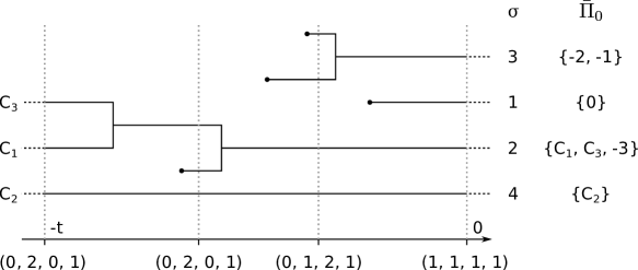
Figure 2: In this example, we have $\bar{\Pi}_{-t}=(C_{1},C_{2},C_{3})$. Each black circle represents an immigration event, and the lines merge at the coalescence time of the blocks to which they correspond. At $t=0$ the blocks of $\bar{\Pi}_{0}$ are labeled according to the permutation $\sigma$, and the value of $(\operatorname{\mathcal{A}}_{t})_{t\geq 0}$ is given below for some times.

Recall that $(M_{t})_{t\in\mathds{R}}$ stands for the number of blocks of $(\bar{\Pi}_{t})_{t\in\mathds{R}}$ forward in time. For each $t\in\mathds{R}$, we define $N_{t}\coloneqq M_{-t}$, the number of blocks of $(\bar{\Pi}_{t})_{t\in\mathds{R}}$ backwards in time. The process $(N_{t})_{t\geq 0}$ also gives the number of particles of the ancestral process $(\operatorname{\mathcal{A}}_{t})_{t\geq 0}$, that is we have

$$\forall t\geq 0,\;N_{t}=\sum_{i\geq 1}\operatorname{\mathcal{A}}_{t}(i).$$

The following proposition shows that the ancestral process is Markovian. This is a key feature that makes Kingman’s coalescent with immigration easier to study than Kingman’s coalescent with erosion.

Proposition 3.3.

Let $(\operatorname{\mathcal{A}}_{t})_{t\geq 0}$ be the ancestral process associated to Kingman’s coalescent with immigration rate $d$, and let $(N_{t})_{t\geq 0}$ be the number of particles of $(\operatorname{\mathcal{A}}_{t})_{t\geq 0}$. Then $(\operatorname{\mathcal{A}}_{t})_{t\geq 0}$ is a Markov process with initial condition

$$\forall i\leq N_{0},\;\operatorname{\mathcal{A}}_{0}(i)=1,\quad\forall i>N_{0},\;\operatorname{\mathcal{A}}_{0}(i)=0.$$

Moreover, conditionally on $\operatorname{\mathcal{A}}_{t}$:

• each particle gives birth to a new particle of its type at rate $d/N_{t}$.

• each particle dies at rate $(N_{t}-1)/2$.

The proof of Proposition 3.3 can be found in Appendix A, we only sketch it here. The process $(M_{t})_{t\in\mathds{R}}$ is a stationary birth-death process, with rates given in Corollary 2.2. A simple calculation shows that it is actually a reversible process, i.e., with our notation, that $(N_{t})_{t\geq 0}$ is distributed as $(M_{t})_{t\geq 0}$. When $(N_{t})_{t\geq 0}$ jumps from $k$ to $k+1$, a particle has given birth to two particles. By exchangeability of our system, the particle that gives birth is chosen uniformly, i.e., each particle gives birth at the same rate $d/k$. Similarly, when $(N_{t})_{t\geq 0}$ jumps from $k$ to $k-1$ a particle chosen uniformly from the population dies. Thus each particle dies at rate $k(k-1)/(2k)=(k-1)/2$.

Making the above argument rigorous involves counting the number of trajectories of $(\bar{\Pi}_{t})_{t\in\mathds{R}}$ yielding a given trajectory of $(\operatorname{\mathcal{A}}_{t})_{t\geq 0}$. We postpone it until Appendix A.

In order to prove Proposition 3.1, we need to keep track of the number of ancestors of $k$ blocks chosen uniformly from $\bar{\Pi}_{0}$. As we have chosen a uniform labeling of the blocks of $\bar{\Pi}_{0}$, this amounts to considering the process $(\operatorname{\mathcal{A}}_{t}(1),\dots,\operatorname{\mathcal{A}}_{t}(k);\,t\geq 0)$. Proposition 3.3 directly gives us the distribution of this process.

Corollary 3.4.

The process $(\operatorname{\mathcal{A}}_{t}(1),\dots,\operatorname{\mathcal{A}}_{t}(p),N_{t};\,t\geq 0)$ is a Markov process such that conditional on $21[2*{\operatorname{\mathcal{A}}_{t}(1)=a_{1},\dots,\operatorname{\mathcal{A}}_{t}(p)=a_{p},N_{t}=k}$, the process jumps to:

• $(a_{1},\dots,a_{i}+1,\dots,a_{p},k+1)$ at rate $\frac{d}{k}a_{i}$.

• $(a_{1},\dots,a_{i}-1,\dots,a_{p},k-1)$ at rate $\frac{k-1}{2}a_{i}$.

• $(a_{1},\dots,a_{p},k+1)$ at rate $\frac{d}{k}(k-a_{1}-\dots-a_{p})$.

• $(a_{1},\dots,a_{p},k-1)$ at rate $\frac{k-1}{2}(k-a_{1}-\dots-a_{p})$.

Proof.

We see from the expression of the transition rates of $(\operatorname{\mathcal{A}}_{t})_{t\geq 0}$ that the rate at which each particle splits or dies only depends on the rest of the population through the total population size $N_{t}$. This is enough to prove the result. ∎

3.2 Convergence

We now prove that the process $(\operatorname{\mathcal{A}}_{t}(1),\dots,\operatorname{\mathcal{A}}_{t}(p);\,t\geq 0)$ converges to independent critical binary birth-death processes when time is rescaled by a factor $1/\sqrt{n}$. We start with the following lemma.

Lemma 3.5.

Let $M^{n}$ have the stationary distribution of $(M^{n}_{t})_{t\geq 0}$, the number of blocks of Kingman’s coalescent with immigration rate $dn$. The sequence $(M^{n}/\sqrt{n};\,n\geq 1)$ is tight.

Proof.

Let $n\geq 1$ and consider a birth-death process $(X^{n}_{t})_{t\geq 0}$ such that conditional on $21[2*{X^{n}_{t}=k}$, the process jumps to

• $k+1$ at rate $dn$;

• $k-1$ at rate $\mu_{k}$,

where the death rate $\mu_{k}$ is defined as

$$\mu_{k}=\begin{cases}0&\text{ if $k<\sqrt{2dn}+1$,}\\ \frac{(\sqrt{2dn}+1)\sqrt{2dn}}{2}&\text{ else.}\end{cases}$$

The process $(X^{n}_{t}-\lfloor\sqrt{2dn}+1\rfloor;\,t\geq 0)$ is distributed as a simple random walk, reflected at $0$. Thus it admits a geometric stationary distribution with parameter $\gamma_{n}$ given by

$$\gamma_{n}=\frac{2dn}{(\sqrt{2dn}+1)\sqrt{2dn}}=\frac{1}{1+\sqrt{\frac{1}{2dn}}}.$$

This shows that the process $(X^{n}_{t})_{t\geq 0}$ also admits a stationary distribution. If $X^{n}$ has the stationary distribution of $(X^{n}_{t})_{t\geq 0}$, then $X^{n}$ is distributed as $\lfloor\sqrt{2dn}\rfloor+1+Y^{n}$, where $Y^{n}$ has a geometric distribution with parameter $\gamma_{n}$.

Hence, for $K$ and $n$ large enough, we have

$$\mathds{P}_{\!#1}^{#2}\left(X^{n}\leq K\sqrt{n}\right) \leq\mathds{P}_{\!#1}^{#2}\left(Y^{n}\leq K\sqrt{n}-\sqrt{2dn}\right)$$

$$=1-\gamma_{n}^{(K-\sqrt{2d})\sqrt{n}}$$

$$=1-\exp(-\frac{K-\sqrt{2d}}{\sqrt{2d}})+o_{n}(1).$$

Thus the sequence $(X^{n}/\sqrt{n};\,n\geq 1)$ is tight.

Recall that $(M^{n}_{t})_{t\geq 0}$ is a birth-death process jumping from $k$ to $k+1$ at rate $dn$, and from $k$ to $k-1$ at rate $k(k-1)/2\geq\mu_{k}$. Its stationary distribution is thus dominated by that of $X^{n}$, and this proves the result. ∎

We now prove our main convergence result. The proof will use a result from Chapter 11 of Ethier and Kurtz (1986) on the a.s. convergence of rescaled Markov processes. In order to stick to their notation, we introduce

$$\forall t\geq 0,\;\hat{N}^{n}_{t}=N^{n}_{t/\sqrt{n}},\quad\,\hat{\!\operatorname{\mathcal{A}}\,}{\!}^{n}_{t}=\operatorname{\mathcal{A}}^{n}_{t/\sqrt{n}},$$

and

$$\forall x\geq 0,\;\beta_{+}(x)=d,\;\beta_{-}(x)=\frac{x^{2}}{2},\;F(x)=d-\frac{x^{2}}{2}$$

Proposition 3.6.

Let $(\operatorname{\mathcal{A}}^{n}_{t})_{t\geq 0}$ be the ancestral process of Kingman’s coalescent with immigration rate $dn$. Then

$$\big{(}\,\hat{\!\operatorname{\mathcal{A}}\,}{\!}^{n}_{t}(1),\dots,\,\hat{\!\operatorname{\mathcal{A}}\,}{\!}^{n}_{t}(p),\frac{\hat{N}^{n}_{t}}{\sqrt{n}};\,t\geq 0\big{)}\Longrightarrow\big{(}X_{1}(t),\dots,X_{p}(t),\sqrt{2d};\,t\geq 0\big{)},$$

in the sense of convergence in distribution in the Skorohod space, and where the processes $(X_{1},\dots,X_{p})$ are i.i.d. critical binary birth-death processes, with per-capita birth and death rate $\sqrt{d/2}$.

Proof.

We start by showing that the process $(\hat{N}^{n}_{t}/\sqrt{n};\,t\geq 0)$ converges to the constant process with value $\sqrt{2d}$. The process $(\hat{N}^{n}_{t})_{t\geq 0}$ is a Markov process jumping from

• $k$ to $k+1$ at rate $d\sqrt{n}=\sqrt{n}\beta_{+}(\frac{k}{\sqrt{n}})$.

• $k$ to $k-1$ at rate $\frac{k(k-1)}{2\sqrt{n}}=\sqrt{n}\beta_{-}(\frac{k}{\sqrt{n}})-\frac{1}{2\sqrt{n}}$.

Thus, the process $(\hat{N}^{n}_{t})_{t\geq 0}$ is of the same form as the processes considered in Theorem 2.1 of Chapter 11 of Ethier and Kurtz (1986), except that the scaling is $\sqrt{n}$ and not $n$.

Let us consider a stationary version of the process $(\hat{N}^{n}_{t})_{t\geq 0}$. Lemma 3.5 shows that the sequence $(\hat{N}^{n}_{0}/\sqrt{n};\,n\geq 1)$ is tight. We can thus find an increasing sequence of indices $(n_{k})_{k\geq 1}$ such that the subsequence $(\hat{N}^{n_{k}}_{0}/\sqrt{n_{k}};\,k\geq 1)$ converges in distribution to a limiting variables $N$. Using Skorohod’s representation theorem (see e.g. Billingsley, 1999), we can assume that the convergence holds a.s.

Applying Theorem 2.1 of Chapter 11 of Ethier and Kurtz (1986) shows that the sequence of processes $(\hat{N}^{n_{k}}_{t}/\sqrt{n_{k}};\,t\geq 0,k\geq 1)$ converges a.s. uniformly on compact sets to the solution of

$$\dot{x}=F(x)=d-\frac{x^{2}}{2},$$ (2)

started from the random variables $N$. (The original theorem is given for a different scaling, but the proof is easily adapted to ours.) As each process $(\hat{N}^{n_{k}}_{t})_{t\geq 0}$ is stationary, the limiting process is a stationary solution to (2), i.e., is the constant process with value $\sqrt{2d}$. This shows that each converging subsequence of $(\hat{N}^{n}_{t}/\sqrt{n};\,t\geq 0,n\geq 1)$ converges to the same constant process, and thus that the entire sequence converges.

Let us now prove the convergence of the ancestral processes. Consider independent Poisson processes $(P^{-}_{i}(t))_{t\geq 0}$, $(P^{+}_{i}(t))_{t\geq 0}$ for $i\leq p$, and $(P^{-}_{N}(t))_{t\geq 0}$, $(P^{+}_{N}(t))_{t\geq 0}$. Using e.g. Theorem 4.1 from Chapter 6 of Ethier and Kurtz (1986), there exists a unique strong solution to the following equation

$$\forall t\geq 0,\forall i\leq p,\;X^{n}_{i}(t)=P^{+}_{i}\Big{(}\int_{0}^{t}\frac{d\sqrt{n}X^{n}_{i}(s)}{Y^{n}(s)}\operatorname{\mathrm{d}\!}s\Big{)}-P^{-}_{i}\Big{(}\int_{0}^{t}\frac{X^{n}_{i}(s)(Y^{n}(s)-1)}{2\sqrt{n}}\operatorname{\mathrm{d}\!}s\Big{)},$$

$$Y^{n}(t)=P^{+}_{N}\Big{(}\int_{0}^{t}d\sqrt{n}(1-\tfrac{\sum_{i}X_{i}^{n}(s)}{Y^{n}(s)})\operatorname{\mathrm{d}\!}s\Big{)}-P^{-}_{N}\Big{(}\int_{0}^{t}\tfrac{Y^{n}(s)(Y^{n}(s)-1)}{2\sqrt{n}}(1-\tfrac{\sum_{i}X^{n}_{i}(s)}{Y^{n}(s)})\operatorname{\mathrm{d}\!}s\Big{)}+\sum_{i=1}^{p}X^{n}_{i}(t).$$

Moreover, this solution $(X^{n}_{1},\dots,X^{n}_{p},Y^{n})$ is distributed as $(\,\hat{\!\operatorname{\mathcal{A}}\,}{\!}^{n}_{t}(1),\dots,\,\hat{\!\operatorname{\mathcal{A}}\,}{\!}^{n}_{t}(p),\hat{N}^{n}_{t};\,t\geq 0)$.

As $Y^{n}/\sqrt{n}$ converges in probability to the constant process with value $\sqrt{2d}$, we can find a subsequence such that

$$\lim_{n\to\infty}\frac{d\sqrt{n}}{Y^{n}(t)}=\sqrt{\frac{d}{2}},\quad\lim_{n\to\infty}\frac{(Y^{n}(t)-1)}{2\sqrt{n}}=\sqrt{\frac{d}{2}}\quad\text{a.s.}$$

holds uniformly in $t$ on compact sets. This is sufficient to show that for each $i\leq p$, the subsequence of processes $(X^{n}_{i}(t))_{t\geq 0}$ converges a.s. in the Skorohod space to the solution $(X_{i}(t))_{t\geq 0}$ of

$$\forall t\geq 0,\forall i\leq p,\;X_{i}(t)=P^{+}_{i}\Big{(}\int_{0}^{t}\sqrt{\frac{d}{2}}X_{i}(s)\operatorname{\mathrm{d}\!}s\Big{)}-P^{-}_{i}\Big{(}\int_{0}^{t}\sqrt{\frac{d}{2}}X_{i}(s)\operatorname{\mathrm{d}\!}s\Big{)}.$$

This proves that the entire sequence $(X^{n}_{1},\dots,X^{n}_{p})$ converges in probability in the Skorohod topology to the solution of the previous equation. Finally, noting that the solutions of these equations are independent and distributed as critical binary branching processes with branching rate $\sqrt{d/2}$ ends the proof. ∎

We are now ready to prove Proposition 3.1.

Proof of Proposition 3.1.

By construction, the size of $p$ blocks of $\bar{\Pi}^{n}$ chosen uniformly is given by the total number of particles of the processes $(\,\hat{\!\operatorname{\mathcal{A}}\,}{\!}^{n}_{t}(1),\dots,\,\hat{\!\operatorname{\mathcal{A}}\,}{\!}^{n}_{t}(p);\,t\geq 0)$. Thus, in the limit, the size of these blocks converges to the total size of $p$ independent critical binary branching processes. ∎

4 Proof of Theorem 1.4

In the previous section we have derived the limiting distribution of the sizes of blocks uniformly sampled from Kingman’s coalescent with immigration. In this section we make use of the coupling between Kingman’s coalescent with immigration and Kingman’s coalescent with erosion from Section 2.3 to get the analogous result in the erosion case.

We first show the following result.

Corollary 4.1.

Let $\Pi^{n}$ have the stationary distribution of the $n$-Kingman coalescent with erosion. Let $(\lvert C^{n}_{1}\rvert,\dots,\lvert C^{n}_{p}\rvert)$ be the size of $p$ blocks chosen uniformly from $\Pi^{n}$. Then

$$(\lvert C^{n}_{1}\rvert,\dots,\lvert C^{n}_{p}\rvert)\Longrightarrow(J_{1},\dots,J_{p}),$$

where $(J_{1},\dots,J_{p})$ are i.i.d. variables distributed as the total progeny of a critical binary branching process.

Proof.

Recall the coupling between Kingman’s coalescent with erosion and Kingman’s coalescent with immigration. Let $(T_{i})_{i\in\mathds{Z}}$ be the atoms of a Poisson point process $P^{n}$ with intensity $dn$, labeled in increasing order such that $T_{0}<0<T_{1}$. Consider an independent i.i.d. sequence of marks $(\ell_{i})_{i\in\mathds{Z}}$ that are uniformly distributed on $[n]$.

Let $\bar{\Pi}^{n}_{0}$ be the value at time $0$ of the version of Kingman’s coalescent with erosion rate $nd$ built from $(T_{i})_{i\in\mathds{Z}}$ as in Section 2.1. We know from Proposition 2.6 that we can obtain a version $\Pi^{n}$ of the stationary distribution of the $n$-Kingman coalescent with erosion by placing $i$ and $j$ in the same block of $\Pi^{n}$ if the last atoms of $P^{n}$ in $\left(-\infty,0\right]$ with mark $i$ and $j$ both belong to the same block of $\bar{\Pi}^{n}_{0}$.

Now let $(\bar{C}_{1}^{n},\dots,\bar{C}^{n}_{p})$ be $p$ blocks chosen uniformly from $\bar{\Pi}_{0}$, and let $(\lvert\bar{C}^{n}_{1}\rvert,\dots,\lvert\bar{C}^{n}_{p}\rvert)$ be their respective sizes. For $k\leq p$, let

$$\lvert C^{n}_{k}\rvert=\operatorname{Card}21[2*{i\in\bar{C}^{n}_{k}\text{$(T_{i},\ell_{i})$ is the last atom in $\left(-\infty,0\right]$ with mark $\ell_{i}$}}.$$

Then conditionally on $21[2*{\lvert C^{n}_{1}\rvert\geq 1,\dots,\lvert C^{n}_{p}\rvert\geq 1}$, $(\lvert C^{n}_{1}\rvert,\dots,\lvert C^{n}_{p}\rvert)$ are the sizes of $p$ blocks chosen uniformly from $\Pi^{n}$. The result is thus proved if we can show that

$$\lim_{n\to\infty}\mathds{P}_{\!#1}^{#2}\left(\lvert C^{n}_{1}\rvert=\lvert\bar{C}^{n}_{1}\rvert,\dots,\lvert C^{n}_{p}\rvert=\lvert\bar{C}^{n}_{p}\rvert\right)=1.$$

Let us first explain intuitively why the previous claim holds. The ancestors of $\bar{C}^{n}_{1}$ have all immigrated on a time-scale of order $1/\sqrt{n}$. On this time-scale, there are of order $\sqrt{n}$ particles that have also immigrated. All these particles receive a uniform label in $[n]$. Thus the probability that an ancestor of $\bar{C}^{n}_{1}$ has received the same label as one of the other $\sqrt{n}$ particles, i.e., that it is not the first atom with its mark, is of order $1/\sqrt{n}$. Let us make this argument rigorous.

Set

$$\tau^{n}_{1}\coloneqq\min 21[2*{T_{i}i\in\bar{C}^{n}_{1}}$$

to be the total life-time of the ancestors of the block $\bar{C}^{n}_{1}$. (The variable $\tau^{n}_{1}$ gives the immigration time of the first particle that forms the block $\bar{C}^{n}_{1}$.) The total number of particles that have immigrated during the time interval $[\tau^{n}_{1},0]$ is then $P^{n}([\tau^{n}_{1},0])$. Consider the event

$$E_{k}=21[2*{\lvert\bar{C}^{n}_{1}\rvert=k,\;\tau^{n}_{1}\in[-\tfrac{t}{\sqrt{n}},0],\;P^{n}([-\tfrac{t}{\sqrt{n}},0])\leq(1+\varepsilon)dt\sqrt{n}}.$$

On this event, if $\lvert C^{n}_{1}\rvert\neq\lvert\bar{C}^{n}_{1}\rvert$, then one the $k$ ancestors of $\bar{C}^{n}_{1}$ has received the same label as one of the particle that has immigrated in the time interval $[\tau^{n}_{1},0]$, that is, the same label as one of the $(1+\varepsilon)dt\sqrt{n}$ last atoms of $P^{n}$. As the labels are chosen uniformly, the probability that the $k$ ancestors all have labels distinct from the labels of the $(1+\varepsilon)dt\sqrt{n}$ last particles is

$$\Big{(}1-\frac{1}{n}\Big{)}\dots\Big{(}1-\frac{k-1}{n}\Big{)}\Big{(}1-\frac{k}{n}\Big{)}^{(1+\varepsilon)dt\sqrt{n}-k}$$

which goes to $1$ as $n$ goes to infinity for all fixed $k$. Thus

$$\mathds{P}_{\!#1}^{#2}\left(\lvert C^{n}_{1}\rvert\neq\lvert\bar{C}^{n}_{1}\rvert,E_{k}\right)\leq\Big{(}1-\frac{1}{n}\Big{)}\dots\Big{(}1-\frac{k-1}{n}\Big{)}\Big{(}1-\frac{k}{n}\Big{)}^{(1+\varepsilon)dt\sqrt{n}-k},$$

and

$$\mathds{P}_{\!#1}^{#2}\left(\lvert C^{n}_{1}\rvert\neq\lvert\bar{C}^{n}_{1}\rvert\right)\leq\; \mathds{P}_{\!#1}^{#2}\left(\tau^{n}_{1}\not\in[-\tfrac{t}{\sqrt{n}},0]\right)+\mathds{P}_{\!#1}^{#2}\left(\lvert\bar{C}^{n}_{1}\rvert\geq K\right)$$

$$+\mathds{P}_{\!#1}^{#2}\left(P^{n}([-\tfrac{t}{\sqrt{n}},0])>(1+\varepsilon)dt\sqrt{n}\right)+o_{n}(1).$$

Now, by Proposition 3.1, the sequence $(-\sqrt{n}\tau^{n}_{1})_{n\geq 1}$ converges in distribution to the total life-time of a binary critical branching process, and $(\lvert\bar{C}^{n}_{1}\rvert)_{n\geq 1}$ converges to the total progeny of this process. Thus, the first two terms in the above equation can be made as small as desired uniformly in $n$ by taking $t$ and $K$ large enough. Using Chebishev’s inequality, the last term can also be made small by choosing a large enough $\varepsilon$. This proves the result for $p=1$ and a simple union bound proves the result for any $p$. ∎

Remark 4.2.

In the previous proof, on the event $21[2*{\lvert\bar{C}^{n}_{1}\rvert=\lvert C^{n}_{1}\rvert}$, not only the size of the blocks of Kingman’s coalescents with erosion and immigration coincide, but also the genealogy of the blocks. Thus we have shown the slightly stronger result that, in the $n$-Kingman coalescent with erosion, the genealogy of a block chosen uniformly from the stationary distribution converges to that of a critical binary branching process.

We can now prove Theorem 1.4. Recall that $\mu^{n}_{k}$ denotes the frequency of blocks of size $k$ of $\Pi^{n}$, i.e., if the blocks of $\Pi^{n}$ are $(C^{n}_{1},\dots,C^{n}_{M^{n}})$, then

$$\mu^{n}_{k}=\frac{1}{M^{n}}\operatorname{Card}(21[2*{i\lvert C^{n}_{i}\rvert=k}).$$

Proof of Theorem 1.4.

(i) We start by proving that $M^{n}/\sqrt{n}$ converges to $\sqrt{2d}$ in probability. Let us consider a version $\bar{\Pi}^{n}$ of the stationary distribution of Kingman’s coalescent with immigration rate $nd$, coupled with a version $\Pi^{n}$ of the stationary distribution of Kingman’s coalescent with erosion rate $d$ on $[n]$. Let $\bar{M}^{n}$, resp. $M^{n}$, denote the number of blocks of $\bar{\Pi}^{n}$, resp. $\Pi^{n}$. Recall that the blocks of $\Pi^{n}$ are subsets of the blocks of $\bar{\Pi}^{n}$, where a particle is retained if there are no other particles with the same label that have immigrated after it. Let $\lvert\bar{C}^{n}\rvert$ be the size of a block of $\bar{\Pi}^{n}$ chosen uniformly, and let $\lvert C^{n}\rvert$ be the size of the corresponding block of $\Pi^{n}$. Some blocks of $\bar{\Pi}^{n}$ are only composed of particles that are not retained to form $\Pi^{n}$. Such blocks have no corresponding blocks in $\Pi^{n}$, and $\bar{M}^{n}-M^{n}$ is exactly the number of such blocks. Thus

$$\mathds{E}\big{[}\frac{\bar{M}^{n}-M^{n}}{\bar{M}^{n}}\big{]}=\mathds{P}_{\!#1}^{#2}\left(\lvert C^{n}\rvert=0\right)\longrightarrow 0.$$

This shows that $M^{n}/\bar{M}^{n}$ goes to $1$ in probability. Lemma 3.5 further shows that $\bar{M}^{n}/\sqrt{n}$ goes to $\sqrt{2d}$ in probability, and thus that $M^{n}/\sqrt{n}$ also goes to $\sqrt{2d}$ in probability.

(ii) We prove the second point using the method of moments. Let $(\lvert C^{n}_{1}\rvert,\dots,\lvert C^{n}_{p}\rvert)$ be the sizes of $k$ uniformly sampled blocks of $\Pi^{n}$. Then, as the number of blocks $M^{n}$ goes to infinity, we have that

$$\lim_{n\to\infty}\mathds{E}[(\mu^{n}_{k})^{p}]=\lim_{n\to\infty}\mathds{P}_{\!#1}^{#2}\left(\lvert C^{n}_{1}\rvert=\dots=\lvert C^{n}_{p}\rvert=k\right)=\mathds{P}_{\!#1}^{#2}\left(J=k\right)^{p},$$

where $J$ is the total progeny of a binary critical branching process. The convergence of the moments readily implies convergence in distribution as the limit is a Dirac mass. ∎

5 Asymptotic frequencies of Kingman’s coalescent with erosion

In this section we prove Theorem 1.3, which gives a representation of the asymptotic frequencies in terms of hierarchically independent diffusions. First, we use the flow of bridges construction of Kingman’s coalescent with erosion from Corollary 2.7 to give a correspondence between the frequencies of the blocks and the size of the families of a Fleming-Viot process.

5.1 Eves of a Fleming-Viot process

Let $(\rho_{t})_{t\geq 0}$ be a Fleming-Viot process. For each individual $x\in[0,1]$, denote

$$\zeta(x)=\inf 21[2*{t\geq 0\rho_{t}(21[2*{x})=0}$$

the extinction time of the offspring of $x$. It is clear that the set

$$21[2*{x\in[0,1]\zeta(x)>0}=21[2*{x\in[0,1]\text{$\rho_{t}(21[2*{x})>0$ for some $t\geq 0$}}$$

is countable. The elements of this set can actually be enumerated in decreasing order of their extinction time, that is, they can be written $(\operatorname{\mathbf{e}}_{i})_{i\geq 0}$ with

$$\zeta(\operatorname{\mathbf{e}}_{1})>\zeta(\operatorname{\mathbf{e}}_{2})>\dots$$

This fact can be found e.g. in Labbé (2014), Theorem 1.6. The sequence $(\operatorname{\mathbf{e}}_{i})_{i\geq 0}$ is called the sequence of Eves of $(\rho_{t})_{t\geq 0}$, and was introduced in Bertoin and Le Gall (2003) and Labbé (2014), see also Duquesne and Labbé (2014) for a similar notion for Continuous-State Branching Processes. The following result shows that the frequencies of the blocks of the stationary distribution of Kingman’s coalescent with erosion can be recovered from the size of the offspring of the Eves.

Lemma 5.1.

Let $(\operatorname{\mathbf{e}}_{i})_{i\geq 1}$ be the Eves of a Fleming-Viot process $(\rho_{t})_{t\geq 0}$. Then the non-increasing reordering of the sequence $(z_{i})_{i\geq 1}$ defined as

$$\forall i\geq 1,\;z_{i}=\int_{0}^{\infty}de^{-dt}\rho_{t}(21[2*{\operatorname{\mathbf{e}}_{i}})\operatorname{\mathrm{d}\!}t$$

is distributed as the frequencies of the blocks of the stationary distribution of Kingman’s coalescent with erosion rate $d$.

Proof.

Consider a flow of bridges $(B_{s,t})_{s\leq t}$, and let $(T_{i})_{i\geq 1}$, $(U_{i})_{i\geq 1}$ be two independent i.i.d. sequences of exponential variables with parameter $d$, and uniform variables respectively. Again, let $\Pi$ be the partition of $\mathds{N}$ defined as

$$i\sim_{\Pi}j\iff B^{-1}_{-T_{i},0}(U_{i})=B^{-1}_{-T_{j},0}(U_{j}),$$

which has the stationary distribution of Kingman’s coalescent with erosion. We denote $\Pi=(C_{1},C_{2},\dots)$ the blocks of $\Pi$, ordered in increasing order of their least elements, i.e., such that

$$i\leq j\iff\min(C_{i})\leq\min(C_{j}).$$

Then let us call

$$A_{i}=B^{-1}_{-T_{j},0}(U_{j}),\;\forall j\in C_{i},$$

the ancestor of the block $C_{i}$.

As the flow of bridges $(B_{s,t})_{s\leq t}$ is independent of the sequences $(U_{i})_{i\geq 1}$ and $(T_{i})_{i\geq 1}$, the sequence $(B^{-1}_{-T_{i},0}(U_{i}))_{i\geq 1}$ is exchangeable. Thus, the law of large numbers shows that for any $i\geq 1$,

$$\frac{1}{n}\operatorname{Card}(C_{i}\cap[n])=\frac{1}{n}\sum_{j=1}^{n}\mathds{1}_{\left\{B^{-1}_{-T_{j},0}(U_{j})=A_{i}\right\}}\underset{n\to\infty}{\longrightarrow}\int_{0}^{\infty}de^{-dt}\rho_{t}(21[2*{A_{i}})\operatorname{\mathrm{d}\!}t\quad\text{a.s.}$$

Thus the result is proved if we can show that a.s.

$$21[2*{\operatorname{\mathbf{e}}_{i}i\geq 1}=21[2*{A_{i}i\geq 1}.$$

Clearly we have $\zeta(A_{i})>0$, as otherwise the frequency of the block $C_{i}$ would be zero. Moreover, conditionally on the flow of bridges, there exists a.s. some $j\geq 1$ such that

$$(U_{j},T_{j})\in 21[2*{(x,t)B^{-1}_{-t,0}(x)=\operatorname{\mathbf{e}}_{i}}$$

as by definition of $\operatorname{\mathbf{e}}_{i}$ this set has positive Lebesgue measure. Thus, a.s. $\operatorname{\mathbf{e}}_{i}$ is the ancestor of some block of $\Pi$, and the result is proved. ∎

In order to prove Theorem 1.3, it remains to show that the sequence of processes $\big{(}\rho_{t}(21[2*{\operatorname{\mathbf{e}}_{1}}),\allowbreak\rho_{t}(21[2*{\operatorname{\mathbf{e}}_{2}}),\dots;\,t\geq 0\big{)}$ has the same distribution as the sequence of hierarchically independent diffusions introduced in Section 1.3. In the following section we characterize this distribution, and complete the proof in the last section.

5.2 Wright-Fisher diffusion conditioned on its extinction order

Consider a $n$-dimensional Wright-Fisher diffusion $(X_{1},\dots,X_{n})$. That is, $(X_{1},\dots,X_{n})$ is distributed as the unique solution to

$$\forall i\geq 1,\;\operatorname{\mathrm{d}\!}X_{i}=\sum_{\begin{subarray}{c}j=1\\ j\neq i\end{subarray}}^{n}\sqrt{X_{i}X_{j}}\operatorname{\mathrm{d}\!}W_{i,j},$$

where $(W_{i,j})_{i<j}$ are independent Brownian motions, and $W_{j,i}=-W_{i,j}$, and started from an initial condition $(x_{1},\dots,x_{n})\in\left(0,1\right)^{n}$ verifying $x_{1}+\dots+x_{n}=1$. The Wright-Fisher diffusion describes the dynamics of a population with constant size, where individuals can be of $n$ different types; $X_{i}$ denotes the frequency of type $i$ individuals in the population. Each process $X_{i}$ is eventually absorbed at $0$ or $1$. We say that the family $X_{i}$ reaches fixation if it gets absorbed at $1$, and that it becomes extinct otherwise. Let

$$\zeta_{i}=\inf 21[2*{t\geq 0X_{i}=0}$$

denote its absorption time at $0$.

In this section, we study the distribution of $(X_{1},\dots,X_{n})$ conditionally on the event $21[2*{\zeta_{n}<\dots<\zeta_{1}}$. First, notice that as $X_{1}+\dots+X_{n}=1$, there is exactly one family that reaches fixation. Thus, on the event $21[2*{\zeta_{n}<\dots<\zeta_{1}}$, we have $\zeta_{1}=\infty$ and $X_{1}$ reaches fixation; $X_{2}$ is the last family to go extinct, and $X_{n}$ is the first family to go extinct. We now express the distribution of the conditioned Wright-Fisher diffusion in terms of the diffusions introduced in Section 1.3.

We will work inductively, by first conditioning the process $(X_{1},\dots,X_{n})$ on $\zeta_{1}$ being the largest extinction time, then on $\zeta_{2}$ being the second largest and so on and so forth. The key point is that after conditioning on the fixation of $X_{1}$, the remainder of the population, $(X_{2},\dots,X_{n})$, is distributed as a rescaled, time-changed, unconditioned $(n-1)$-dimensional Wright-Fisher diffusion, independent of $X_{1}$.

Let us be more specific and let $Y_{1}$ be the solution of

$$\operatorname{\mathrm{d}\!}Y_{1}=(1-Y_{1})\operatorname{\mathrm{d}\!}t+\sqrt{Y_{1}(1-Y_{1})}\operatorname{\mathrm{d}\!}W_{1},$$ (3)

for some Brownian motion $W_{1}$. Notice that $Y_{1}$ is distributed as a usual $1$-dimensional Wright-Fisher diffusion, conditioned on fixation. Consider the fixation time of $Y_{1}$ which is defined as

$$S_{1}=\inf 21[2*{t\geq 0Y_{1}(t)=1}.$$

We further define a random time-change $\tau_{1}$ as

$$\forall t<S_{1},\;\tau_{1}(t)=\int_{0}^{t}\frac{1}{1-Y_{1}(s)}\operatorname{\mathrm{d}\!}s,\quad\forall t\geq S_{1},\;\tau_{1}(t)=\infty.$$

We start by proving the following result.

Lemma 5.2.

Let $Y_{1}$ and $\tau_{1}$ be as above and consider an independent $(n-1)$-dimensional Wright-Fisher diffusion $(X_{2},\dots,X_{n})$. Then, the process $(Z_{1},\dots,Z_{n})$ defined as

$$Z_{1}=Y_{1},\quad\forall i>1,\forall t\geq 0,\;Z_{i}(t)=(1-Z_{1}(t))X_{i}(\tau_{1}(t)),$$

is distributed as a $n$-dimensional Wright-Fisher diffusion conditioned on $21[2*{\zeta_{1}=\infty}$.

Remark 5.3.

The time $\tau_{1}(t)$ is infinite with positive probability. However, each of the processes $(X_{2},\dots,X_{n})$ has an a.s. limit as $t$ goes to infinity. On the event $21[2*{\tau_{1}(t)=\infty}$, we take $X_{i}(\tau_{1}(t))$ to be this limit, so that the process $(Z_{1},\dots,Z_{n})$ is now well-defined.

Before proving Lemma 5.2, we need the following fact that we prove for the sake of completeness.

Lemma 5.4.

Let $(W_{t})_{t\geq 0}$ be a Brownian motion on $\mathds{R}$ started at $1$, and let $T_{0}$ be the first time it hits $0$. Then for $\alpha\in\mathds{R}$, a.s.

$$\int_{0}^{T_{0}}W_{s}^{\alpha}\operatorname{\mathrm{d}\!}s=\begin{cases}\infty&\text{ if $\alpha\leq-2$}\\ y_{\alpha}<\infty&\text{ if $\alpha>-2$.}\end{cases}$$

Proof.

Let us define

$$\forall t\geq 0,\;\xi_{t}=\tilde{W}_{t}-\frac{t}{2},\quad\tau(t)=\inf\Big{\{}s\geq 0:\int_{0}^{s}\exp(2\xi_{u})\operatorname{\mathrm{d}\!}u>t\Big{\}},$$

for a Brownian motion $(\tilde{W}_{t})_{t\geq 0}$ with the convention that $\inf\mathchoice{\ooalign{$\displaystyle\mathrm{O}$\cr\raise 1.03334pt\hbox{$\displaystyle\not{}$}\cr}}{\ooalign{$\textstyle\mathrm{O}$\cr\raise 0.94722pt\hbox{$\textstyle\not{}$}\cr}}{\ooalign{$\scriptstyle\mathrm{O}$\cr\raise 0.6458pt\hbox{$\scriptstyle\not{}$}\cr}}{\ooalign{$\scriptscriptstyle\mathrm{O}$\cr\raise 0.38748pt\hbox{$\scriptscriptstyle\not{}$}\cr}}=\infty$ and $\xi_{\infty}=-\infty$. The Lamperti representation of positive self-similar processes (Lamperti, 1972) shows that $W_{t}$ stopped at $T_{0}$ satisfies the equality in distribution

$$(W_{t\wedge T_{0}})_{t\geq 0}\overset{\mathrm{(d)}}{=}(\exp(\xi_{\tau(t)}))_{t\geq 0}.$$

Thus

$$\int_{0}^{t\wedge T_{0}}W_{s}^{\alpha}\operatorname{\mathrm{d}\!}s\overset{\mathrm{(d)}}{=}\int_{0}^{t}\exp(\alpha\xi_{\tau(s)})\operatorname{\mathrm{d}\!}s=\int_{0}^{\tau(t)}\exp((2+\alpha)\xi_{s})\operatorname{\mathrm{d}\!}s,$$

and

$$\int_{0}^{T_{0}}W_{s}^{\alpha}\operatorname{\mathrm{d}\!}s\overset{\mathrm{(d)}}{=}\int_{0}^{\infty}\exp((2+\alpha)\xi_{s})\operatorname{\mathrm{d}\!}s,$$

which yields the result. ∎

Proof of Lemma 5.2.

Consider a $n$-dimensional Wright-Fisher diffusion $(X_{1},\dots,X_{n})$. A calculation of Doob’s $h$-transform using the harmonic function

$$h(x_{1},\dots,x_{n})=\mathds{P}_{\!#1}^{#2}\left(\lim_{t\to\infty}X_{1}(t)=1\nonscript\>\middle|\nonscript\>\mathopen{}X_{1}(0)=x_{1},\dots,X_{n}(0)=x_{n}\right)=x_{1}$$

shows that the process $(X_{1},\dots,X_{n})$ conditioned on $21[2*{\lim_{t\to\infty}X_{1}(t)=1}=21[2*{\zeta_{1}=\infty}$ is distributed as the unique solution to the equation

$$\operatorname{\mathrm{d}\!}X_{1}=(1-X_{1})\operatorname{\mathrm{d}\!}t+\sum_{\begin{subarray}{c}j=2\end{subarray}}^{n}\sqrt{X_{1}X_{j}}\operatorname{\mathrm{d}\!}W_{1,j},$$

$$\forall i\geq 2,\;\operatorname{\mathrm{d}\!}X_{i}=-X_{i}\operatorname{\mathrm{d}\!}t+\sum_{\begin{subarray}{c}j=1\\ j\neq i\end{subarray}}^{n}\sqrt{X_{i}X_{j}}\operatorname{\mathrm{d}\!}W_{i,j},$$

where $(W_{i,j})_{i<j}$ are independent Brownian motions, and $W_{i,j}=-W_{j,i}$. We will prove that the process $(Z_{1},\dots,Z_{n})$ solves this equation.

Now consider a $(n-1)$-dimensional Wright-Fisher diffusion $(X^{\prime}_{2},\dots,X^{\prime}_{n})$ independent of $Y_{1}$ which solves

$$\forall i\geq 2,\;\operatorname{\mathrm{d}\!}X^{\prime}_{i}=\sum_{\begin{subarray}{c}j=2\\ j\neq i\end{subarray}}^{n}\sqrt{X^{\prime}_{i}X^{\prime}_{j}}\operatorname{\mathrm{d}\!}W^{\prime}_{i,j}.$$

We start by giving the equation solved by the process $(Y_{1},X^{\prime}_{2}\circ\tau_{1},\dots,X^{\prime}_{n}\circ\tau_{1})$. Notice that here, only a subset of the processes are time-changed, and that $\tau_{1}$ explodes in finite time. For these two reasons, let us realize the time-change carefully.

We transform $\tau_{1}$ into a family of finite stopping times. Our first task is to prove that $\tau_{1}$ goes continuously to infinity, we do this using the speed and scale measures of the diffusion $Y_{1}$, see e.g. Etheridge (2011). If we define $D=1/Y_{1}$, then

$$\operatorname{\mathrm{d}\!}D=\sqrt{D-1}D\operatorname{\mathrm{d}\!}W_{1},\quad\forall t\geq 0,\;[D,D]_{t}=\int_{0}^{t}(D(s)-1)D(s)^{2}\operatorname{\mathrm{d}\!}s.$$

Thus we can write that

$$\int_{0}^{S_{1}}\frac{1}{1-Y_{1}(s)}\operatorname{\mathrm{d}\!}s=\int_{0}^{S_{1}}\frac{D(s)}{D(s)-1}\operatorname{\mathrm{d}\!}s\overset{\mathrm{(d)}}{=}\int_{0}^{S_{1}}\frac{W_{1}([D,D]_{s})}{W_{1}([D,D]_{s})-1}\operatorname{\mathrm{d}\!}s=\int_{0}^{T_{1}}\frac{1}{(W_{1}(s)-1)^{2}W_{1}(s)}\operatorname{\mathrm{d}\!}s$$

where $W_{1}$ is a Brownian motion started at $1/Y_{1}(0)$, and $T_{1}$ is the first time when $W_{1}$ hits $1$. We now know from Lemma 5.4 that this integral is a.s. infinite, and thus that $\tau_{1}$ goes continuously to infinity, and does not “jump to infinity”.

Further consider the times

$$\forall i\geq 2,\;S_{i}=\inf 21[2*{t\geq 0X^{\prime}_{i}(t)=1},\quad S=\min(S_{2},\dots,S_{n}).$$

At time $S$, one of the families has reached fixation, and thus for $t\geq S$ we have $X^{\prime}_{i}(t)=X^{\prime}_{i}(S)$. Therefore, for all $t\geq 0$, we have $X^{\prime}_{i}(\tau_{1}(t))=X^{\prime}_{i}(\tau_{1}(t)\wedge S)$, where the stopping time $\tau_{1}(t)\wedge S$ is now a.s. finite, and $t\mapsto\tau_{1}(t)\wedge S$ is continuous. (The continuity requires that $\tau_{1}$ does not jump to infinity.) Thus, by making a time-change in the following integrals, see e.g. Kallenberg (2002), Theorem 17.24, we obtain

$$\forall t\geq 0,\;X^{\prime}_{i}(\tau_{1}(t)) =X^{\prime}_{i}(\tau_{1}(t)\wedge S)$$

$$=\sum_{\begin{subarray}{c}j=2\\ j\neq i\end{subarray}}^{n}\int_{0}^{\tau_{1}(t)\wedge S}\sqrt{X^{\prime}_{i}(s)X^{\prime}_{j}(s)}\operatorname{\mathrm{d}\!}W_{i,j}$$

$$=\sum_{\begin{subarray}{c}j=2\\ j\neq i\end{subarray}}^{n}\int_{0}^{t}\sqrt{X^{\prime}_{i}(\tau_{1}(s)\wedge S)X^{\prime}_{j}(\tau_{1}(s)\wedge S)}\operatorname{\mathrm{d}\!}W_{i,j}(\tau_{1}(s)\wedge S)$$

$$=\sum_{\begin{subarray}{c}j=2\\ j\neq i\end{subarray}}^{n}\int_{0}^{t}\sqrt{\frac{X^{\prime}_{i}(\tau_{1}(s))X^{\prime}_{j}(\tau_{1}(s))}{1-Y_{1}(s)}}\operatorname{\mathrm{d}\!}\tilde{W}_{i,j}$$

where

$$\forall t\geq 0,\;\tilde{W}_{i,j}(t)=\int_{0}^{t}\sqrt{1-Y_{1}(s)}\operatorname{\mathrm{d}\!}W_{i,j}(\tau_{1}(s)\wedge S).$$

A direct computation of the quadratic variations gives

$$\forall i,j,t\geq 0,\;[\tilde{W}_{i,j},\tilde{W}_{i,j}]_{t}=t\wedge S,$$

and the crossed variations are null. Thus a multidimensional version of Dubins-Schwarz theorem, see e.g. Theorem 18.4 in Kallenberg (2002), shows that we can find independent Brownian motions $(\hat{W}_{i,j})_{i<j}$ such that $\tilde{W}_{i,j}(t)=\hat{W}_{i,j}(t\wedge S)$. This proves that the time-changed processes solve

$$\forall t\geq 0,\;X^{\prime}_{i}(\tau_{1}(t))=\sum_{\begin{subarray}{c}j=2\\ j\neq i\end{subarray}}^{n}\int_{0}^{t}\sqrt{\frac{X^{\prime}_{i}(\tau_{1}(s))X^{\prime}_{j}(\tau_{1}(s))}{1-Y_{1}(s)}}\operatorname{\mathrm{d}\!}\hat{W}_{i,j}.$$

A final application of Itô’s formula shows that the process $(Z_{1},\dots,Z_{n})$ as defined above solves the same equation as $(X_{1},\dots,X_{n})$ conditioned on $21[2*{\zeta_{1}=\infty}$. This proves the result. ∎

We can now proceed inductively. Let us set up the notation for the proof. Consider i.i.d. processes $(Y_{1},\dots,Y_{n-1})$ such that

$$\forall i\geq 1,\;\operatorname{\mathrm{d}\!}Y_{i}=(1-Y_{i})\operatorname{\mathrm{d}\!}t+\sqrt{Y_{i}(1-Y_{i})}\operatorname{\mathrm{d}\!}W_{i}$$

where $(W_{1},\dots,W_{n-1})$ are independent Brownian motions. We set $\tilde{Z}_{1}=Y_{1}$, and

$$\forall t\geq 0,\;\tilde{\tau}_{1}(t)=\int_{0}^{t}\frac{1}{1-\tilde{Z}_{1}(s)}\operatorname{\mathrm{d}\!}s.$$

We then define recursively, for $i<n-1$,

$$\forall t\geq 0,\;\tilde{Z}_{i+1}(t)=(1-\tilde{Z}_{1}(t)-\dots-\tilde{Z}_{i}(t))Y_{i+1}(\tilde{\tau}_{i}(t))$$

$$\forall t\geq 0,\;\tilde{\tau}_{i+1}(t)=\int_{0}^{t}\frac{1}{1-\tilde{Z}_{1}(s)-\dots-\tilde{Z}_{i+1}(s)}\operatorname{\mathrm{d}\!}s.$$

We finally set $\tilde{Z}_{n}=1-\tilde{Z}_{1}-\dots-\tilde{Z}_{n-1}$.

Proposition 5.5.

The process $(\tilde{Z}_{1},\dots,\tilde{Z}_{n})$ defined above is distributed as a $n$-dimensional Wright-Fisher diffusion conditioned on $21[2*{\zeta_{n}<\dots<\zeta_{1}}$.

Proof.

We prove the result inductively. For $n=2$, conditioning $(X_{1},X_{2})$ on its extinction order amounts to conditioning it on the fixation of $X_{1}$, and Lemma 5.2 shows that the result holds.

Let $(Y_{1},\dots,Y_{n-1})$ be the i.i.d. diffusions defined above. We first define

$$\forall t\geq 0,\;\tilde{Z}^{\prime}_{2}(t)=Y_{2}(t),\quad\forall t\geq 0,\;\tau^{\prime}_{2}(t)=\int_{0}^{t}\frac{1}{1-\tilde{Z}^{\prime}_{2}(s)}\operatorname{\mathrm{d}\!}s$$

and then define inductively, for $i<n-1$,

$$\forall t\geq 0,\;\tilde{Z}^{\prime}_{i+1}(t)=(1-\tilde{Z}^{\prime}_{2}(t)-\dots-\tilde{Z}^{\prime}_{i}(t))Y_{i+1}(\tilde{\tau}_{i}^{\prime}(t)),$$

$$\forall t\geq 0,\;\tilde{\tau}^{\prime}_{i+1}(t)=\int_{0}^{t}\frac{1}{1-\tilde{Z}^{\prime}_{2}(s)-\dots-\tilde{Z}^{\prime}_{i+1}(s)}\operatorname{\mathrm{d}\!}s,$$

and $\tilde{Z}^{\prime}_{n}=1-\tilde{Z}^{\prime}_{2}-\dots-\tilde{Z}^{\prime}_{n-1}$. By induction, we can suppose that $(\tilde{Z}^{\prime}_{2},\dots,\tilde{Z}^{\prime}_{n})$ is distributed as a $(n-1)$-dimensional Wright-Fisher diffusion conditioned on its extinction order. We first claim that the process defined as

$$\forall t\geq 0,\;\tilde{Z}_{1}(t)=Y_{1}(t),$$

$$\forall i>1,\forall t\geq 0,\;\tilde{Z}_{i}(t)=(1-\tilde{Z}_{1}(t))\tilde{Z}^{\prime}_{i}(\tilde{\tau}_{1}(t))$$

is distributed as a $n$-dimensional Wright-Fisher diffusion conditioned on its extinction order.

To see this, let $(X_{2},\dots,X_{n})$ be a $(n-1)$-dimensional unconditioned Wright-Fisher diffusion, independent of $Y_{1}$, and recall the definition of $(Z_{1},\dots,Z_{n})$ from Lemma 5.2. Consider

$$\zeta^{\prime}_{i}=\inf 21[2*{t\geq 0Z_{i}(t)=0},\quad\zeta_{i}=\inf 21[2*{t\geq 0X_{i}(t)=0}$$

the extinction times of $Z_{i}$ and $X_{i}$. Lemma 5.2 ensures that $(Z_{1},\dots,Z_{n})$ is distributed as a Wright-Fisher diffusion conditioned on the fixation of $Z_{1}$. Thus, the process $(Z_{1},\dots,Z_{n})$ further conditioned on $21[2*{\zeta^{\prime}_{n}<\dots<\zeta^{\prime}_{2}}$ has the distribution of a Wright-Fisher diffusion conditioned on its extinction order. Now notice that

$$21[2*{\zeta^{\prime}_{n}<\dots<\zeta^{\prime}_{2}}=21[2*{\zeta_{n}<\dots<\zeta_{2}}.$$

Thus conditioning $(Z_{1},\dots,Z_{n})$ on $21[2*{\zeta^{\prime}_{n}<\dots\zeta^{\prime}_{2}}$ amounts to conditioning $(X_{2},\dots,X_{n})$ on $21[2*{\zeta_{n}<\dots<\zeta_{2}}$, that is, conditioning it on its fixation order. As $21[2*{\zeta_{n}<\dots<\zeta_{2}}$ is independent of $Z_{1}$, conditioning the process $(Z_{1},\dots,Z_{n})$ on this event is equivalent to replacing $(X_{2},\dots,X_{n})$ by $(\tilde{Z}^{\prime}_{2},\dots,\tilde{Z}^{\prime}_{n})$ in the construction of $(Z_{1},\dots,Z_{n})$, and this proves the claim.

It only remains to show that $\tilde{Z}_{i+1}$ as defined in the proof can be written

$$\forall i>1,\;\tilde{Z}_{i+1}(t)=(1-\tilde{Z}_{1}(t)-\dots-\tilde{Z}_{i}(t))Y_{i}(\tilde{\tau}_{i}(t)).$$

A direct calculation first shows that

$$\forall i>1,\;\forall t\geq 0,\;\tilde{\tau}_{i}(t)=\tilde{\tau}^{\prime}_{i}(\tilde{\tau}_{1}(t))$$

and the result follows. ∎

We end this section by pointing out the following fact that will be required in the next section. We have only defined the Wright-Fisher diffusion conditioned on its extinction order for an initial condition $(x_{1},\dots,x_{n})$ such that for all $1\leq i\leq n$, $x_{i}>0$. Nevertheless, the processes $Y_{i}$ have an entrance boundary at $0$. Thus there exists a unique extension of the process $(Y_{1},\dots,Y_{n-1})$ started from $(0,\dots,0)$ that remains Feller, see e.g. Kallenberg (2002), Chapter 23. This shows that a Wright-Fisher diffusion conditioned on its fixation order $(\tilde{Z}_{1},\dots,\tilde{Z}_{n})$ admits a Feller extension for the initial condition $(0,\dots,0,1)$.

5.3 Proof of Theorem 1.3

Let $(\rho_{t})_{t\geq 0}$ be a Fleming-Viot process, and let $(\operatorname{\mathbf{e}}_{i})_{i\geq 1}$ be its Eves. In this section we end the proof of Theorem 1.3 by showing that the distribution of the sequence of processes $(\rho_{t}(21[2*{\operatorname{\mathbf{e}}_{1}}),\rho_{t}(21[2*{\operatorname{\mathbf{e}}_{2}}),\dots;\,t\geq 0)$ is that of a Wright-Fisher diffusion conditioned on its fixation order.

The result we want to prove is the direct extension of Theorem 4 of Bertoin and Le Gall (2003). Reformulated in our setting, this theorem proves that $(\rho_{t}(21[2*{\operatorname{\mathbf{e}}_{1}});\,t\geq 0)$ is distributed as the solution to eq. 3 started from $0$. We now give a similar representation for the process $(\rho_{t}(21[2*{\operatorname{\mathbf{e}}_{1}}),\dots,\rho_{t}(21[2*{\operatorname{\mathbf{e}}_{n}});\,t\geq 0)$ giving the size of the progeny of the first $n$ Eves.

Proposition 5.6.

Let $(\rho_{t})_{t\geq 0}$ be a Fleming-Viot process, and $(\operatorname{\mathbf{e}}_{i})_{i\geq 1}$ be its Eves. Then for any $n\geq 1$, the process $(\rho_{t}(21[2*{\operatorname{\mathbf{e}}_{1}}),\dots,\rho_{t}(21[2*{\operatorname{\mathbf{e}}_{n}});\,t\geq 0)$ is distributed as $(\tilde{Z}_{1},\dots,\tilde{Z}_{n})$ where $(\tilde{Z}_{1},\dots,\tilde{Z}_{n+1})$ is a $(n+1)$-dimensional Wright-Fisher diffusion conditioned on its extinction order, started from $(0,\dots,0,1)$.

Proof.

We realize a similar computation as in the proof of Theorem 4 of Bertoin and Le Gall (2003). The proof requires three facts. First notice that

$$\lim_{m\to\infty}\rho_{t}\big{(}\big{(}\textstyle\frac{\left\lfloor m\operatorname{\mathbf{e}}_{i}\right\rfloor}{m},\frac{\left\lfloor m\operatorname{\mathbf{e}}_{i}+1\right\rfloor}{m}\big{]}\big{)}=\rho_{t}(21[2*{\operatorname{\mathbf{e}}_{i}}).$$

Then, if $I_{1},\dots,I_{n}$ are $n$ disjoint intervals of length $1/m$, due to exchangeability of the increments of bridges, the process $(\rho_{t}(I_{1}),\dots,\rho_{t}(I_{n});\,t\geq 0)$ is distributed as the process

$$\textstyle\Big{(}\rho_{t}\big{(}\left(0,\frac{1}{m}\right]\big{)},\dots,\rho_{t}\big{(}\left(\frac{n-1}{m},\frac{n}{m}\right]\big{)};\,t\geq 0\Big{)}$$

which is distributed as the $n$ first coordinates of a $(n+1)$-dimensional Wright-Fisher diffusion started from $(\tfrac{1}{m},\dots,\tfrac{1}{m},1-\tfrac{n}{m})$.

Finally, notice that on the event $21[2*{\forall i\neq j\in 21[2*{1,\dots,n},\;\left\lfloor m\operatorname{\mathbf{e}}_{i}\right\rfloor\neq\left\lfloor m\operatorname{\mathbf{e}}_{j}\right\rfloor}$, conditioning the process

$$\textstyle\Big{(}\rho_{t}\big{(}\left(0,\frac{1}{m}\right]\big{)},\dots,\rho_{t}\big{(}\left(\frac{n-1}{m},\frac{n}{m}\right]\big{)};\,t\geq 0\Big{)}$$

on its extinction order as in Section 5.2 is equivalent to conditioning it on the location of the Eves, i.e., on the event $21[2*{\forall k\in 21[2*{1,\dots,n},\;\operatorname{\mathbf{e}}_{k}\in\left(\frac{k-1}{m},\frac{k}{m}\right]}$.

We can now proceed to the calculation. Let $0\leq t_{1}<\dots<t_{p}$ and let $\varphi_{1},\dots,\varphi_{p}$ be continuous bounded functions. Consider $(\tilde{Z}_{1},\dots,\tilde{Z}_{n+1})$ a $(n+1)$-dimensional Wright-Fisher diffusion conditioned on its extinction order. Then

$$\mathds{E}\Big{[}\varphi_{1}\big{(}\rho_{t_{1}}(21[2*{\operatorname{\mathbf{e}}_{1}}),\dots,\rho_{t_{1}}(21[2*{\operatorname{\mathbf{e}}_{n}})\big{)}\dots\varphi_{p}\big{(}\rho_{t_{p}}(21[2*{\operatorname{\mathbf{e}}_{1}}),\dots,\rho_{t_{p}}(21[2*{\operatorname{\mathbf{e}}_{n}})\big{)}\Big{]}$$

$$=\lim_{m\to\infty}\sum_{i_{1}=0}^{m-1}\dots\sum_{i_{n}=0}^{m-1}\textstyle\mathds{E}\Big{[}\varphi_{1}\big{(}\rho_{t_{1}}\big{(}\left(\frac{i_{1}}{m},\frac{i_{1}+1}{m}\right]\big{)},\dots,\rho_{t_{1}}\big{(}\left(\frac{i_{n}}{m},\frac{i_{n}+1}{m}\right]\big{)}\big{)}\dots$$

$$\textstyle\qquad\qquad\qquad\qquad\quad\;\;\,\varphi_{p}\big{(}\rho_{t_{p}}\big{(}\left(\frac{i_{1}}{m},\frac{i_{1}+1}{m}\right]\big{)},\dots,\rho_{t_{p}}\big{(}\left(\frac{i_{n}}{m},\frac{i_{n}+1}{m}\right]\big{)}\big{)}\mathds{1}_{\left\{\forall k\in 21[2*{1,\dots,n},\;\operatorname{\mathbf{e}}_{k}\in\left(\frac{i_{k}}{m},\frac{i_{k}+1}{m}\right]\right\}}\Big{]}$$

$$=\lim_{m\to\infty}m^{n}\textstyle\mathds{E}\Big{[}\varphi_{1}\big{(}\rho_{t_{1}}\big{(}\left(0,\frac{1}{m}\right]\big{)},\dots,\rho_{t_{1}}\big{(}\left(\frac{n-1}{m},\frac{n}{m}\right]\big{)}\big{)}\dots$$

$$\textstyle\quad\qquad\qquad\quad\varphi_{p}\big{(}\rho_{t_{p}}\big{(}\left(0,\frac{1}{m}\right]\big{)},\dots,\rho_{t_{p}}\big{(}\left(\frac{n-1}{m},\frac{n}{m}\right]\big{)}\big{)}\mathds{1}_{\left\{\forall k\in 21[2*{1,\dots,n},\;\operatorname{\mathbf{e}}_{k}\in\left(\frac{k-1}{m},\frac{k}{m}\right]\right\}}\Big{]}$$

$$=\lim_{m\to\infty}\textstyle\mathds{E}\Big{[}\varphi_{1}\big{(}\tilde{Z}_{1}(t_{1}),\dots,\tilde{Z}_{n}(t_{1})\big{)}\dots\varphi_{p}\big{(}\tilde{Z}_{1}(t_{p}),\dots,\tilde{Z}_{n}(t_{p})\big{)}\;|\;\tilde{Z}_{1}(0)=\dots=\tilde{Z}_{n}(0)=\frac{1}{m}\Big{]}$$

$$=\mathds{E}\Big{[}\varphi_{1}\big{(}\tilde{Z}_{1}(t_{1}),\dots,\tilde{Z}_{n}(t_{1})\big{)}\dots\varphi_{p}\big{(}\tilde{Z}_{1}(t_{p}),\dots,\tilde{Z}_{n}(t_{p})\big{)}\;|\;\tilde{Z}_{1}(0)=\dots=\tilde{Z}_{n}(0)=0\Big{]},$$

where, the last line comes from the Feller property of the process $(\tilde{Z}_{1},\dots,\tilde{Z}_{n+1})$. ∎

Our current proof of Theorem 1.3 relies on calculations specific to the Wright-Fisher diffusion. We end this section by discussing a potential alternative proof of this result that would more easily generalize to Beta-coalescents.

The Feller branching diffusion describes the size of a population where different individuals die and reproduce independently. Similarly to the Fleming-Viot process, it is possible to define a measure-valued process, called the Dawson-Watanabe process, that encodes the size of the offspring of each individual in the initial population, see e.g. Etheridge (2000). (Note that there are no mutations here, i.e., no spatial motion of the particles.) Its total mass is then distributed as a Feller diffusion. Starting from a Dawson-Watanabe process, one can renormalize it by its total mass to obtain a process valued in the space of probability measures. Then the resulting renormalized process is distributed as a time-changed Fleming-Viot process, see Birkner et al. (2005).

Let us now discuss the results of Section 5.2 in the light of this new construction. The key point of Section 5.2 is that after removing one family from a Fleming-Viot process and renormalizing the remainder of the population to have mass one, the resulting process remains distributed as an independent time-changed Fleming-Viot process. Suppose that the Fleming-Viot process has been obtained by renormalizing a Dawson-Watanabe process. Then removing a family from the Fleming-Viot process amounts to removing a family from the original Dawson-Watanabe process. By the branching property, removing this family does not change the distribution of the remainder of the population, which remains distributed as an independent Dawson-Watanabe process. Thus when renormalizing the remainder of the population to have size one, we obtain a new time-changed Fleming-Viot process, independent of the removed family. In other words, the results of Section 5.2 essentially originate from the fact that the Fleming-Viot process can be seen as a renormalized branching measure-valued process.

A similar link has been obtained in Birkner et al. (2005) between the $\Lambda$-Fleming-Viot processes associated to Beta-coalescents and a family of $\alpha$-stable measure-valued branching processes. Thus we believe that one could derive a similar, but less explicit, representation of the asymptotic frequencies of the stationary distribution of the Beta-coalescents with erosion than the one obtained in Theorem 1.3.

Appendix A Proof of Proposition 3.3

In this section, we prove that the ancestral process of Kingman’s coalescent with immigration is Markovian. To do this, consider a version of Kingman’s coalescent with immigration $(\bar{\Pi}_{t})_{t\in\mathds{R}}$, and let $(\bar{\Pi}_{i})_{i\in\mathds{Z}}$ be its embedded chain, i.e., the sequence of states visited by $(\bar{\Pi}_{t})_{t\in\mathds{R}}$, where $\bar{\Pi}_{0}$ is the state at time $t=0$. We count the number of trajectories of $(\bar{\Pi}_{i})_{i\in\mathds{Z}}$ that produce a given trajectory of $(\operatorname{\mathcal{A}}_{i})_{i\geq 0}$, the embedded chain of $(\operatorname{\mathcal{A}}_{t})_{t\geq 0}$.

First, note that given the values of $(\bar{\Pi}_{-n},\dots,\bar{\Pi}_{0})$ and a uniform permutation $\sigma$ of the blocks of $\bar{\Pi}_{0}$, one can uniquely reconstruct the values of $(\operatorname{\mathcal{A}}_{0},\dots,\operatorname{\mathcal{A}}_{n})$. We now fix a sequence $(a_{0},\dots,a_{n})$ of possible values of $(\operatorname{\mathcal{A}}_{0},\dots,\operatorname{\mathcal{A}}_{n})$, and a partition $\bar{\pi}_{-n}$ with $\lvert a_{n}\rvert$ blocks, where $\lvert a_{n}\rvert$ is the total number of particles of $a_{n}$. Our first task is to count the number of trajectories of $(\bar{\Pi}_{-n},\dots,\bar{\Pi}_{0})$ starting from $\bar{\pi}_{-n}$, and of labelings $\sigma$ of the blocks of $\bar{\Pi}_{0}$ such that $(\operatorname{\mathcal{A}}_{0},\dots,\operatorname{\mathcal{A}}_{n})=(a_{0},\dots,a_{n})$. Before stating the result we need to introduce one notation. The variable $\operatorname{\mathcal{A}}_{k+1}$ is obtained from $\operatorname{\mathcal{A}}_{k}$ by splitting or killing one particle. Let us denote $\ell_{k}$ the label of this particle. That is, $\ell_{k}$ is the unique integer such that

$$\lvert\operatorname{\mathcal{A}}_{k+1}(\ell_{k})-\operatorname{\mathcal{A}}_{k}(\ell_{k})\rvert=1,\quad\forall i\neq\ell_{k},\;\lvert\operatorname{\mathcal{A}}_{k+1}(i)-\operatorname{\mathcal{A}}_{k}(i)\rvert=0.$$

Lemma A.1.

Fix a sequence of states $(a_{0},\dots,a_{n})$ of $(\operatorname{\mathcal{A}}_{0},\dots,\operatorname{\mathcal{A}}_{n})$, and a partition $\bar{\pi}_{-n}$ of $21[2*{i\in\mathds{Z}i\leq-n}$ with $\left\lvert a_{n}\right\rvert$ blocks. Then the number of trajectories of $(\bar{\Pi}_{-n},\dots,\bar{\Pi}_{0})$ and labelings of the blocks of $\bar{\Pi}_{0}$ such that $(\operatorname{\mathcal{A}}_{0},\dots,\operatorname{\mathcal{A}}_{n})=(a_{0},\dots,a_{n})$ and $\bar{\Pi}_{-n}=\bar{\pi}_{-n}$ is

$$\frac{\left\lvert a_{n}\right\rvert!}{2^{b}}a_{0}(\ell_{0})\dots a_{n-1}(\ell_{n-1}),$$

where $b$ is the number of birth events along the sequence $(a_{0},\dots,a_{n})$.

Proof.

Each trajectory of $(\bar{\Pi}_{-n},\dots,\bar{\Pi}_{0})$ naturally encodes a forest that can be built as follows. Choose any labeling of the blocks of $\bar{\Pi}_{-n}$, and for each block add an initial leaf with the corresponding label. Suppose that the forest corresponding to $(\bar{\Pi}_{-n},\dots,\bar{\Pi}_{-k})$ has been built. If $\bar{\Pi}_{-k+1}$ is obtained from $\bar{\Pi}_{-k}$ by immigrating a new particle, then add a new isolated vertex. Otherwise, a coalescence event has occurred between two blocks of $\bar{\Pi}_{-k}$. Then add a new internal node and connect it to the nodes corresponding to the two blocks that have coalesced. Once the forest representing $(\bar{\Pi}_{-n},\dots,\bar{\Pi}_{0})$ is built, by construction the nodes corresponding to $\bar{\Pi}_{0}$ all belong to different trees. We set them to be the roots of their respective trees, and label them according to the partition $\sigma$. (Notice that the resulting forest is endowed with some additional structure: the nodes added along the procedure are totally ordered by the induction step at which they have been added.)

Counting trajectories of $(\bar{\Pi}_{-n},\dots,\bar{\Pi}_{0})$ now amounts to counting forests. Instead of building the forests by starting from the leaves as above, we build a forest with ancestral sequence $(a_{0},\dots,a_{n})$ by starting from the roots. Initially, consider a set of $\left\lvert a_{0}\right\rvert$ roots, labeled by $21[2*{1,\dots,\left\lvert a_{0}\right\rvert}$, that represent the particles of $a_{0}$. Nodes can be in two states: active or inactive. Active nodes represent the particles that are still alive in the population while inactive nodes represent the dead particles. Initialy all roots are active. We build the forest recursively. Suppose that at step $k$ we have built a forest such that for all $i$ there are $a_{k}(i)$ nodes that are active in the tree with root $i$. If a particle with label $\ell_{k}$ has died from $a_{k}$ to $a_{k+1}$, we inactivate one of the nodes belonging to the tree with root $\ell_{k}$. There are $a_{k}(\ell_{k})$ such nodes. Similarly, if a particle has split from $a_{k}$ to $a_{k+1}$, we inactivate one node in the tree $\ell_{k}$, and connect it to two new active nodes. There are again $a_{k}(\ell_{k})$ active nodes in the tree $\ell_{k}$. After step $n$, we have built a forest with ancestral sequence $(a_{0},\dots,a_{n})$. We assign the blocks of $\bar{\Pi}_{-n}$ to the remaining active nodes of the forest by choosing one of the $\left\lvert a_{n}\right\rvert!$ permutations of the blocks.

There are

$$\left\lvert a_{n}\right\rvert!\,a_{0}(\ell_{0})\dots a_{n-1}(\ell_{n-1})$$

outputs of the previous construction, and all forests with ancestral sequence $(a_{0},\dots,a_{n})$ can be obtained that way. However, due to symmetries, some forests can be obtained multiple times through this construction. More precisely, at each birth events, the two daughter nodes are indistinguishable. Interchanging the trees corresponding to the offspring of these two nodes yields the same forest. Thus, the actual number of forests with ancestral sequence $(a_{0},\dots,a_{n})$ is

$$\frac{\left\lvert a_{n}\right\rvert!}{2^{b}}a_{0}(\ell_{0})\dots a_{n-1}(\ell_{n-1})$$

where $b$ is the number of birth events, and the result is proved. ∎

Lemma A.2.

Let $(M_{t})_{t\in\mathds{R}}$ be the process counting the number of blocks of Kingman’s coalescent with immigration. Then $(M_{t})_{t\in\mathds{R}}$ is a reversible process.

Proof.

Let us compute the stationary distribution of $(M_{t})_{t\in\mathds{R}}$. As $(M_{t})_{t\in\mathds{R}}$ jumps from $k$ to $k+1$ at rate $d$ and from $k$ to $k-1$ at rate $k(k-1)/2$, a usual calculation shows that its stationary distribution $(\nu_{k})_{k\geq 1}$ is

$$\forall k\geq 1,\;\nu_{k}\propto\frac{(2d)^{k}}{k!\,(k-1)!}$$

where the renormalization constant is obtained by summing over all the terms. Thus a direct calculation now proves that $(\nu_{k})_{k\geq 1}$ fulfills the detailed balance equation

$$\forall k\geq 1,\;d\nu_{k}=\frac{k(k+1)}{2}\nu_{k+1}$$

and thus that $(M_{t})_{t\in\mathds{R}}$ is reversible. ∎

We are now ready to prove Proposition 3.3

Proof of Proposition 3.3.

Recall the notations from Section 3.1. As proved in Lemma A.2, the process $(M_{t})_{t\in\mathds{R}}$ that counts the number of the blocks of Kingman’s coalescent with immigration is a reversible Markov process. Thus, the process $(N_{t})_{t\geq 0}$ that gives the number of particles of $(\operatorname{\mathcal{A}}_{t})_{t\geq 0}$ is a stationary process jumping from $k$ to $k+1$ at rate $d$, and from $k$ to $k-1$ at rate $k(k-1)/2$. Hence, the result is proved if we show that conditional on $(N_{0},\dots,N_{n})$, the type of the particle that dies or splits from $\operatorname{\mathcal{A}}_{k}$ to $\operatorname{\mathcal{A}}_{k+1}$ is chosen with a probability proportional to the vector $\operatorname{\mathcal{A}}_{k}$. We have

$$\mathds{P}_{\!#1}^{#2}\left(\operatorname{\mathcal{A}}_{0}=a_{0},\dots,\operatorname{\mathcal{A}}_{n}=a_{n}\right)=\sum_{(\bar{\pi}_{-n},\dots,\bar{\pi}_{0})}\sum_{s}\mathds{P}_{\!#1}^{#2}\left(\forall i<n,\;\bar{\Pi}_{-i}=\bar{\pi}_{-i},\;\sigma=s\nonscript\>\middle|\nonscript\>\mathopen{}\bar{\Pi}_{-n}=\bar{\pi}_{-n}\right)\mathds{P}_{\!#1}^{#2}\left(\bar{\Pi}_{-n}=\bar{\pi}_{-n}\right)$$

where the sum is taken over all partitions $\bar{\pi}_{-n}$ of $21[2*{i\in\mathds{Z}i\leq-n}$ with $\lvert a_{0}\rvert$ blocks, all trajectories $(\bar{\pi}_{-n+1},\dots,\bar{\pi}_{0})$ and labelings $s$ of the blocks of $\bar{\pi}_{0}$ such that $(\operatorname{\mathcal{A}}_{0},\dots,\operatorname{\mathcal{A}}_{n})=(a_{0},\dots,a_{n})$. Now notice that the probability of seeing such a trajectory and labeling does only depend on the sequence of number of blocks $(\lvert a_{0}\rvert,\dots,\lvert a_{n}\rvert)$. Indeed we have

$$\mathds{P}_{\!#1}^{#2}\left(\forall i<n,\;\bar{\Pi}_{-i}=\bar{\pi}_{-i},\;\sigma=s\nonscript\>\middle|\nonscript\>\mathopen{}\bar{\Pi}_{-n}=\bar{\pi}_{-n}\right)=\frac{1}{\lvert a_{0}\rvert!}\prod_{i=0}^{n-1}\frac{d\mathds{1}_{\left\{\lvert a_{i+1}\rvert-\lvert a_{i}\rvert=-1\right\}}+\mathds{1}_{\left\{\lvert a_{i+1}\rvert-\lvert a_{i}\rvert=1\right\}}}{d+\lvert a_{i+1}\rvert(\lvert a_{i+1}\rvert-1)/2}.$$

Thus the probability of the event $21[2*{\operatorname{\mathcal{A}}_{0}=a_{0},\dots,\operatorname{\mathcal{A}}_{n}=a_{n}}$ is proportional to the number of terms in the sum, and thus to the number of trajectories of $(\bar{\Pi}_{-n},\dots,\bar{\Pi}_{0})$ that correspond to this ancestral sequence. Hence, Lemma A.1 shows that

$$\mathds{P}_{\!#1}^{#2}\left(\operatorname{\mathcal{A}}_{0}=a_{0},\dots,\operatorname{\mathcal{A}}_{n}=a_{n}\right)\propto a_{0}(\ell_{0})\dots a_{n-1}(\ell_{n-1}),$$

where the coefficient only depends on $(\lvert a_{0}\rvert,\dots,\lvert a_{n}\rvert)$. This proves the result. ∎

Let us end this section by discussing a possible extension to $\Lambda$-coalescents. The key point here is that conditionally on the block counting process, the particles that die or split are chosen uniformly in the population. This is a consequence of 1) Lemma A.1 and 2) the fact that all trajectories with a given sequence of number of blocks have the same probability. The second point is a consequence of exchangeability so remains valid for $\Lambda$-coalescents. As for Lemma A.1, the proof could be easily adapted to $\Lambda$-coalescents with immigration. (The factor $2^{b}$ should be replaced by the product of the number of blocks involved in coalescence events.)

Thus, the only difference between Kingman’s coalescent with immigration and more general $\Lambda$-coalescents with immigration is that the block counting process is no longer reversible. Hence we cannot obtain a closed form for the transition rates of the corresponding ancestral processes. Nevertheless, we believe that in some cases it should be possible to obtain a result similar to Theorem 1.4 by using the same techniques as in this paper, if one can derive a good enough approximation for the stationary distribution of the number of blocks.

References

- Berestycki (2004) J. Berestycki. Exchangeable fragmentation-coalescence processes and their equilibrium measures. Electronic Journal of Probability, 9:770–824, 2004. doi:10.1214/EJP.v9-227.
- Bertoin (2006) J. Bertoin. Random Fragmentation and Coagulation Processes. Cambridge Studies in Advanced Mathematics. Cambridge University Press, 2006. doi:10.1017/CBO9780511617768.
- Bertoin and Le Gall (2003) J. Bertoin and J.-F. Le Gall. Stochastic flows associated to coalescent processes. Probability Theory and Related Fields, 126(2):261–288, 2003. doi:10.1007/s00440-003-0264-4.
- Billingsley (1999) P. Billingsley. Convergence of Probability Measures. Wiley Series in Probability and Statistics. John Wiley & Sons, Inc., second edition, 1999. doi:10.1002/9780470316962.
- Birkner et al. (2005) M. Birkner, J. Blath, M. Capaldo, A. Etheridge, M. Möhle, J. Schweinsberg, and A. Wakolbinger. Alpha-stable branching and Beta-coalescents. Electronic Journal of Probability, 10:303–325, 2005. doi:10.1214/EJP.v10-241.
- Duquesne and Labbé (2014) T. Duquesne and C. Labbé. On the Eve property for CSBP. Electronic Journal of Probability, 19:31 pp., 2014. doi:10.1214/EJP.v19-2831.
- Etheridge (2000) A. Etheridge. An Introduction to Superprocesses, volume 20 of University Lecture Series. American Mathematical Society, 2000. doi:10.1090/ulect/020.
- Etheridge (2011) A. Etheridge. Some Mathematical Models from Population Genetics, volume 2012 of École d’Été de Probabilités de Saint-Flour. Springer Science & Business Media, 2011. doi:10.1007/978-3-642-16632-7.
- Ethier and Kurtz (1986) S. N. Ethier and T. G. Kurtz. Markov Processes: Characterization and Convergence. Wiley Series in Probability and Statistics. John Wiley & Sons, Inc., 1986. doi:10.1002/9780470316658.
- Kallenberg (2002) O. Kallenberg. Foundations of Modern Probability. Probability and its Applications. Springer-Verlag New York, second edition, 2002. doi:10.1007/978-1-4757-4015-8.
- Kingman (1982) J. F. Kingman. The coalescent. Stochastic Processes and their Applications, 13:235–248, 1982. doi:10.1016/0304-4149(82)90011-4.
- Labbé (2014) C. Labbé. From flows of -fleming-viot processes to lookdown processes via flows of partitions. Electronic Journal of Probability, 19:49 pp., 2014. doi:10.1214/EJP.v19-3192.
- Lambert (2008) A. Lambert. Population dynamics and random genealogies. Stochastic Models, 24:45–163, 2008. doi:10.1080/15326340802437728.
- Lamperti (1972) J. Lamperti. Semi-stable markov processes. I. Zeitschrift für Wahrscheinlichkeitstheorie und Verwandte Gebiete, 22:205–225, 1972. doi:10.1007/BF00536091.
- Mallet et al. (2016) J. Mallet, N. Besansky, and M. W. Hahn. How reticulated are species? BioEssays, 38:140–149, 2016. doi:10.1002/bies.201500149.
- Pitman (1999) J. Pitman. Coalescents with multiple collisions. Annals of Probability, 27:1870–1902, 1999. doi:10.1214/aop/1022874819.
- Roux et al. (2016) C. Roux, C. Fraïsse, J. Romiguier, Y. Anciaux, N. Galtier, and N. Bierne. Shedding light on the grey zone of speciation along a continuum of genomic divergence. PLOS Biology, 14:1–22, 2016. doi:10.1371/journal.pbio.2000234.
- Sagitov (1999) S. Sagitov. The general coalescent with asynchronous mergers of ancestral lines. Journal of Applied Probability, 36:1116–1125, 1999. doi:10.1239/jap/1032374759.