Optimal paths of non-equilibrium stochastic fields: the Kardar-Parisi-Zhang interface as a test case

Abstract

Atypically large fluctuations in macroscopic non-equilibrium systems continue to attract interest. Their probability can often be determined by the optimal fluctuation method (OFM). The OFM brings about a conditional variational problem, the solution of which describes the “optimal path” of the system which dominates the contribution of different stochastic paths to the desired statistics. The OFM proved efficient in evaluating the probabilities of rare events in a host of systems. However, theoretically predicted optimal paths were observed in stochastic simulations only in diffusive lattice gases, where the predicted optimal density patterns are either stationary, or travel with constant speed. Here we focus on the one-point height distribution of the paradigmatic Kardar-Parisi-Zhang interface. Here the optimal paths, corresponding to the distribution tails at short times, are intrinsically non-stationary and can be predicted analytically. Using the mapping to the directed polymer in a random potential at high temperature, we obtain “snapshots” of the optimal paths in Monte-Carlo simulations which probe the tails with an importance sampling algorithm. For each tail we observe a very narrow “tube” of height profiles around a single optimal path which agrees with the analytical prediction. The agreement holds even at long times, supporting earlier assertions of the validity of the OFM in the tails well beyond the weak-noise limit.

Non-equilibrium behaviors of stochastic macroscopic systems are ubiquitous in nature. One interesting group of questions about such systems concern atypically large fluctuations, which manifest themselves as tails of probability distributions of different fluctuating quantities. Although a universal description of the tails is not likely to emerge, a great progress has been achieved in the last two decades in particular systems. Much of the progress has been due to a method which emerged in different areas of physics under different names: the optimal fluctuation method (OFM), the instanton method, the weak noise theory, the macroscopic fluctuation theory, etc. A key ingredient of this method is a saddle-point evaluation of the path integral of the stochastic process in question, conditioned on the specified large deviation. This evaluation, which employs a model-dependent small parameter (colloquially called “weak noise”), brings about a conditional variational problem. Its solution – a deterministic field, evolving in time – describes the “optimal path”: the most probable history of the system which dominates the contribution to the desired statistics. The OFM has been proved efficient in a host of non-equilibrium problems: turbulence and turbulent transport Falkovich1996 ; GM1996 ; FalkovichRMP ; Chernykh ; Grafke ; Bouchet , stochastic surface growth and related systems Mikhailov1991 ; Fogedby1998 ; KK2007 ; KK2008 ; KK2009 ; FogedbyRen ; MV2016 ; MKV ; KMSparabola ; Janas2016 ; SMS2017 ; MeersonSchmidt2017 ; SMS2018 ; SKM2018 ; MSV_3d ; SmithMeerson2018 ; MV2018 ; Asida2019 ; SMV2019 , diffusive transport in the absence Jona2006 ; Jona2007 ; bertini2015 ; BD2004 ; Bertini2005 ; BD2005 ; Sukhorukov2004 ; Tailleur1 ; Appert ; BDL2008 ; HG2009 ; DG2009b ; HG2011 ; LGW ; Bunin ; KM2012 ; Gorissen2012 ; void ; Akkermans ; MSKMP ; Espirages2013 ; Hurtado2013review ; MSSSEP ; Sadhu ; VMS2014 ; MR ; MVK ; AMV ; ZM ; Espirages2016 ; Baek ; AM2017 ; Baek2 ; ZM ; Baek ; AM2017 ; Baek2 ; narrow ; AKM2019 ; DerridaSadhu2019 and in the presence Elgart ; Basile2004 ; Bodieneau2010 ; MS2011a ; MSKaplan ; MS2011b ; MVS ; Hurtado2013 ; M2015 ; Lasanta of particle reactions or energy dissipation, etc. However, we are aware only of one class of systems – diffusive lattice gases – where theoretically predicted optimal paths were actually observed in stochastic simulations HG2009 ; HG2011 ; Gorissen2012 ; Hurtado2013review ; ZM ; Espirages2016 . Furthermore, in all these systems the optimal density patterns are either stationary, or travel with constant speed.

Here we report (to our knowledge, for the first time) the observation of intrinsically non-stationary optimal paths. We consider the paradigmatic Kardar-Parisi-Zhang (KPZ) equation in 1+1 dimension KPZ :

$$\partial_{t}h=\nu\partial_{x}^{2}h+(\lambda/2)\left(\partial_{x}h\right)^{2}+\sqrt{D}\,\xi(x,t),$$ (1)

where $\nu$ is the diffusivity, and we can set the non-linearity coefficient $\lambda>0$ without loss of generality. Equation (1) describes the evolution of the height $h(x,t)$ of an interface driven by the Gaussian noise $\sqrt{D}\xi(x,t)$ which has zero mean and is delta-correlated: $\langle\xi(x_{1},t_{1})\xi(x_{2},t_{2})\rangle=\delta(x_{1}-x_{2})\delta(t_{1}-t_{2})$. The KPZ equation has been extensively studied KPZ ; HHZ ; Barabasi ; Krug ; S2016 . At long times, the interface width was found to grow as $t^{1/3}$, while the lateral correlation length grows as $t^{2/3}$. The exponents $1/3$ and $2/3$ are the hallmark of a whole universality class of the 1+1 dimensional non-equilibrium growth HHZ ; Barabasi ; Krug ; Corwin ; QS ; S2016 ; Takeuchi2017 .

In the last decade the studies of the KPZ equation and related systems have seen spectacular developments Corwin ; QS ; S2016 ; Takeuchi2017 . They shifted from the interface roughness and correlation function to more detailed characteristics such as the full probability distribution of the interface height at a point, $\mathcal{P}\left(H,t\right)$. Remarkably, exact representations were derived for $\mathcal{P}\left(H,t\right)$ for the KPZ equation on the line $|x|<\infty$ for several basic initial conditions: “droplet” SS2010 ; Calabrese2010 ; Dotsenko2010 ; Amir2011 , flat flat , stationary stationary1 ; stationary2 , and some of their combinations. At long times and for typical height fluctuations, $\mathcal{P}\left(H,t\right)$ converges to the Tracy-Widom (TW) distribution for the Gaussian unitary ensemble (GUE) of random matrices TWGUE for the droplet, to the TW distribution for the Gaussian orthogonal ensemble (GOE) TWGOE for the flat interface, and to the Baik-Rains (BR) distribution BR for the stationary interface. These theoretical predictions were confirmed in ingenious experiments with liquid-crystal turbulent fronts experiment , see also Ref. interpretation . Atypically large fluctuations – the tails of $\mathcal{P}\left(H,t\right)$ – behave differently and are unrelated to the TW and BR distributions. These tails were determined, for the three basic initial conditions and for several other initial conditions, by the OFM KK2007 ; KK2008 ; KK2009 ; MKV ; KMSparabola ; Janas2016 ; MeersonSchmidt2017 ; SKM2018 . The OFM predictions were verified in all cases where the corresponding tails were also extracted from exact representations.

The most thoroughly studied is the droplet case, for which the OFM predicted the following tails KMSparabola :

$$-\ln\mathcal{P}(H,t)\simeq \frac{8\sqrt{2}\,\nu}{3D\lambda^{1/2}}\,\frac{H^{3/2}}{t^{1/2}}, H\to+\infty$$ , (2)

$$-\ln\mathcal{P}(H,t)\simeq \frac{4\sqrt{2\lambda}}{15\pi D}\,\frac{|H|^{5/2}}{t^{1/2}}, H\to-\infty$$ . (3)

The higher tail (2) coincides with the corresponding tail of the GUE TW distribution, while the lower tail (3) is different from the GUE TW tail (the latter scales as $|H|^{3}/t$). Using the exact representations, it was shown that the tails (2) and (3) are observed both at short times DMRS2016 and at long times DMS2016 ; SMP ; Corwinetal ; CorwinGhosal2018a ; KLD2018 ; Tsai ; CorwinGhosal2018b . Furthermore, these tails have been recently verified in rare-event stochastic simulations Hartmann2018 which employed a standard mapping to (a discrete version of) the directed polymer in a random potential at high temperature Huse1985 ; KPZ ; HHZ ; S2016 ; Krug ; CLDR2010 . The problem of the KPZ one-point height statistics in 1+1 dimension for the droplet initial condition can therefore serve as a good test case for the studies of optimal paths in spatially explicit and non-stationary stochastic systems conditioned on large deviations. Here we use the directed polymer mapping and the importance sampling algorithm Hartmann2018 to obtain “snapshots” of the optimal paths. As in the previous work Hartmann2018 , our simulations probe the distribution tails with reaching the probability densities as small as $10^{-1000}$. For each of the two tails we observe a very narrow tube of height profiles around a single optimal path which agrees with an analytical prediction. The agreement holds even at relatively large times, supporting earlier assertions of the validity of the OFM in the tails well beyond the weak-noise limit.

1. Optimal path: theoretical predictions for $h(x,t/2)$. Let us recall the OFM formulation of the problem of one-point KPZ height statistics KK2007 ; MKV ; KMSparabola . For typical fluctuations, the OFM relies on the smallness of the dimensionless parameter $\epsilon=(t/t_{\text{NL}})^{1/2}\ll 1$, where $t_{\text{NL}}=\nu^{5}/(D^{2}\lambda^{4})$ is the characteristic nonlinear time of the KPZ equation. A saddle-point evaluation of the path integral, corresponding to Eq. (1), leads to a variational problem for the action. The resulting Euler-Lagrange equations can be recast in the Hamiltonian form. In the rescaled variables $\tau/t\to\tau$, $x\sqrt{\nu t}\to x$, and $\lambda h/\nu\to h$, the Hamilton’s equations are

$$\partial_{\tau}h = \partial_{x}^{2}h+(1/2)\left(\partial_{x}h\right)^{2}+\rho,$$ (4)

$$\partial_{\tau}\rho = -\partial_{x}^{2}\rho+\partial_{x}\left(\rho\partial_{x}h\right),$$ (5)

where $\rho(x,\tau)$ is the “momentum” density field, canonically conjugate to $h(x,\tau)$; it describes the optimal realization of the noise $\xi(x,t)$. In Ref. KMSparabola a parabolic initial condition $h(x,0)=-x^{2}/L$ was considered. The droplet case follows from these results in the limit of $L\to 0$. The condition $h(x=0,\tau=t)=H$ translates into $\rho(x=0,\tau=t)=\Lambda\,\delta(x)$; the Lagrange multiplier $\Lambda$ is ultimately expressed through $H$. Once the OFM problem is solved, one can calculate the (rescaled) action $s=s(H)=(1/2)\int_{0}^{t}d\tau\int dx\,\rho^{2}(x,\tau)$ and obtain, in the original variables,

$$-\ln\mathcal{P}(H,t)\simeq\frac{\nu^{5/2}}{D\lambda^{2}\sqrt{t}}\,\,s\left(\frac{\lambda H}{\nu}\right).$$ (6)

As the noise magnitude $D$ drops out from the “classical mechanics” formulation, the optimal path – the solution of the OFM problem for $h(x,\tau)$ – is independent of $D$.

As of present, the exact optimal path is unknown, but asymptotic solutions for very large positive and negative $H$ [which determine the tails (2) and (3)] are available KMSparabola . Here are “snapshots” of these asymptotic solutions at $\tau=t/2$. For very large positive $H$

$$\!\!h\left(x,\frac{t}{2}\right)\simeq \frac{H}{2}-\sqrt{\frac{2H}{\lambda t}}\,|x|, |x|\leq\sqrt{\lambda Ht/2}$$ , (7)

$$\!\!h\left(x,\frac{t}{2}\right)\simeq -x^{2}/\lambda t, |x|>\sqrt{\lambda Ht/2}$$ , (8)

see Fig. 1 a. In the leading order in $\lambda H/\nu\gg 1$, $h(x,\tau)$ does not depend on the diffusivity $\nu$. Equation (7) describes a snapshot of two outgoing “ramps” of $h(x,\tau)$, which correspond to a stationary “antishock” of the interface slope $v(x,\tau)=\partial_{x}h(x,\tau)$ at $x=0$, sustained by a very narrow stationary pulse of $\rho$ Fogedby1998 ; KK2007 ; MKV ; KMSparabola . The solution (8) describes the noiseless ($\xi=0$) evolution of the KPZ equation (1) starting from the droplet initial condition. The solutions (7) and (8) are continuous with their first derivatives at the moving boundaries between them KMSparabola . At $\tau=t/2$ these boundaries are at $|x|=\sqrt{\lambda Ht/2}$. If one accounts for the diffusion, the corner singularity of $h(x,t/2)$ at $x=0$ is smoothed MKV :

$$\!\!h\!\left(\!x,\frac{t}{2}\right)\!\simeq\!\frac{H}{2}-\frac{2\nu}{\lambda}\ln\cosh\!\left(\!\sqrt{\frac{\lambda H}{2\nu^{2}t}}\,x\!\right),|x|\leq\sqrt{\frac{\lambda Ht}{2}},$$ (9)

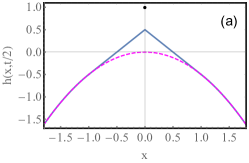
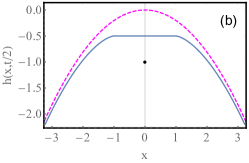
Figure 1: Analytical predictions of optimal paths at $t=1/2$ conditioned on reaching a large positive (a) and negative (b) height $H$ at $x=0$ at time $t$ (denoted by the fat point). (a): prediction of Eqs. (7) and (8); $x$ is rescaled by $\sqrt{\lambda Ht/2}$. (b): prediction of Eqs. (10) and (11); $x$ is rescaled by $\sqrt{2\lambda|H|t}/\pi$. In both panels $h$ is rescaled by $|H|$. The dashed lines, $-x^{2}/2$ (a) and $-2x^{2}/\pi^{2}$ (b), show in the corresponding units the zero-noise KPZ interface at time $t/2$.

For very large negative $H$ the optimal path is quite different. Using the results of Ref. KMSparabola , we obtain

$$\!\!h\left(x,\frac{t}{2}\right)\simeq \frac{H}{2}, |x|\leq\frac{\sqrt{2\lambda|H|t}}{\pi}$$ ​​​​​​, (10)

$$\!\!h\left(x,\frac{t}{2}\right)\simeq \frac{H}{2}\,\mathfrak{h}\left(\frac{\pi\,|x|}{\sqrt{2\lambda|H|t}}\right), |x|\geq\frac{\sqrt{2\lambda|H|t}}{\pi}$$ ​​​​​​, (11)

where the function $\mathfrak{h}(z)$ is defined parametrically, $z(u)=1+u\arctan u,\mathfrak{h}(u)=1+\frac{2}{\pi}\left[u+(u^{2}-1)\arctan u\right]$, $0\leq u<\infty$. Here too the optimal path is independent of $\nu$ in the leading order. Noticeable is an extended flat region of $h(x,t/2)$, see Fig. 1 b. As one can see, the optimal paths for large positive and negative $H$ are strikingly different.

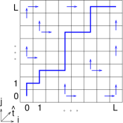
Figure 2: A realization of the directed polymer $(0,0)\to(L,L)$. The arrows indicate samples for possible directions of the polymer for some lattice sites.

2. Directed polymer mapping. Now let us recall the discrete version of the mapping between the KPZ height $h(x,t)$ and the free energy of a directed polymer in a two-dimensional random potential at high temperature $T$ Calabrese2010 . Consider all directed polymers which start at the point $(0,0)$ and end at the point $(L,L)$ of a square lattice indexed by integers $(i,j)$ which run from $0$ to $L$, as shown in Fig. 2. The value of the potential $V$ at each lattice point is normally distributed with zero mean and unit variance. Introduce the new variables $\hat{\tau}=i+j$ and $\hat{x}=(i-j)/2$. The partition function $Z(i,j)$ of a given random configuration of the potential, $Z(i,j)=\hat{Z}[(i-j)/2,i+j]$, with the end point $(i,j)$, obeys the exact recursive equation Calabrese2010

$$\!\hat{Z}\left(\hat{x},\hat{\tau}+1\right)\!=\!\left[\hat{Z}\left(\hat{x}-\frac{1}{2},\hat{\tau}\right)+\hat{Z}\left(\hat{x}+\frac{1}{2},\hat{\tau}\right)\right]\!e^{-\frac{V\left(\hat{x},\hat{\tau}+1\right)}{T}},$$ (12)

where $\left\langle V\left(\hat{x},\hat{\tau}\right)V\left(\hat{x}^{\prime},\hat{\tau}^{\prime}\right)\right\rangle=\delta_{\hat{x}\hat{x}^{\prime}}\delta_{\hat{\tau}\hat{\tau}^{\prime}}$, and $\delta_{\hat{x}\hat{x}^{\prime}}$ and $\delta_{\hat{\tau}\hat{\tau}^{\prime}}$ are Kronecker deltas. Let $Z^{*}\left(\hat{x},\hat{\tau}\right)=2^{-\hat{\tau}}\hat{Z}\left(\hat{x},\hat{\tau}\right)$. The mapping to the continuous Eq. (1) is achieved via a truncated Taylor expansion of all the discrete quantities and $\exp(-V/T)$ in Eq. (12). For example,

$$Z^{*}(\hat{x}-\frac{1}{2},\hat{\tau})=Z^{*}(\hat{x},\hat{\tau})-\frac{1}{2}\partial_{\hat{x}}Z^{*}(\hat{x},\hat{\tau})+\frac{1}{8}\partial_{\hat{x}}^{2}Z^{*}(\hat{x},\hat{\tau})+\dots.$$ (13)

To justify these expansions, we use strong inequalities $L\gg 1$ and $T\gg 1$. This procedure approximates the discrete Eq. (12) by the stochastic heat equation

$$\partial_{\tau}Z^{*}=\frac{1}{8}\partial_{x}^{2}Z^{*}-\frac{\xi}{T}Z^{*},$$ (14)

where we dropped the hats of $\hat{x}$ and $\hat{\tau}$. The (now continuous) noise term $\xi$ is delta-correlated in $x$ and $\tau$. The initial condition is $Z^{*}(x,0)=\delta(x)$. The desired mapping is given by the relations $h(x,\tau)=\ln[Z^{*}(x,\tau)/\langle Z^{*}(0,\tau)\rangle],\lambda=1/4,\nu=1/8$, $D=T^{-2}$ and $t=2L$ Calabrese2010 . The characteristic nonlinear time of the KPZ equation, $t_{\text{NL}}=\nu^{5}/(D^{2}\lambda^{4})$, becomes $T^{4}/2^{7}$.

3. Importance sampling algorithm. The rare-event simulation method used here is based on the idea to bias the underlying distribution towards the outcomes of interest. It was introduced in computer science under the names importance sampling or variance reduction hammersley1956 and has been frequently used in physics, in particular when studying explicitly time-dependent processes with transition-path sampling dellago1998 , cloning approaches giardina2006 or density-matrix renormalization group gorissen2009 . Our approach is more straightforward and somewhat more general, as it applies to a very broad range of stochastic systems, both in and out of equilibrium work_ising2014 .

To obtain realizations of the random field $V$ which correspond to extreme values of $H=H(V)$, we do not sample the random field according to its natural Gaussian product weight $G(V)$, but according to the modified weight $P(V)\sim G(V)\exp(-H/\Theta)$. $\Theta$ is an auxiliary “temperature” parameter, which allows us to shift the peak of distributions to smaller than ($\Theta>0$ close to zero) or larger than ($\Theta<0$ close to zero) typical values. The random realizations cannot be generated directy according to the weight $P(V)$. Instead we use a standard Markov-chain approach with the Metropolis-Hastings algorithm newman1999 , where the configurations of the Markov chain are the random realizations. By sampling for different values of $\Theta$ and combining and normalizing the results, $H$ can be sampled over a larger range of the support Hartmann2018 , down to probabilities like $10^{-1000}$. For details of the approach, see Refs. align2002 ; work_ising2014 ; Hartmann2018 . We extend the approach by storing regularly during the simulation (after equilibration) configurations sampled at various values of $\Theta$. We also extend the simulations to even smaller values of $H$. For configurations exhibiting corresponding values of $H$ of interest we then can analyze $h(x,t/2)$.

4. Simulation results and comparison with theory. In our first series of simulations we chose $L=2^{7}$ and $T^{4}=2^{13}$. Although $\epsilon=(t/t_{\text{NL}})^{1/2}=2$ is not small, the simulations of Ref. Hartmann2018 confirmed the validity of the OFM for the whole distribution $\mathcal{P}(H,t)$. One can expect, therefore, that the OFM predictions of the optimal paths will be accurate. This is indeed what our simulations show. Figure 3 is a result of processing of 10 simulated configurations at $\tau=t/2$, conditioned on reaching a large positive $H$ (close to 21.9) at $\tau=t$. They appear in the natural ensemble with a probability near $10^{-200}$ Hartmann2018 . Instead of showing the 10 actual profiles, we only presented the profile averaged over the realizations and the error bars. As one can see, the error bars are strikingly small, implying a very narrow tube of stochastic trajectories around the optimal path. Furthermore, this optimal path agrees very well with the leading-order (zero-diffusion) analytical prediction (7) and (8), and remarkably well with the finite-diffusion expression (9).

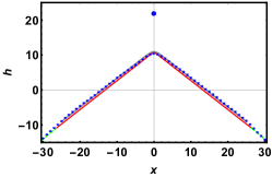
Figure 3: The optimal path at $\tau=t/2$, conditioned on a large positive height $H$ (close to $21.9$, the fat point) at $\tau=t$ for $T^{4}=2^{13}$ and $L=2^{7}$. The symbols with error bars show the results of 10 realizations. The lower solid line is the zero-diffusion solution (7). The higher solid line is the finite-diffusion solution (9). Dashed line: the parabola (8).

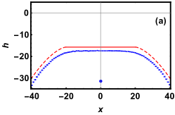
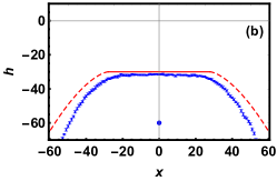
Figure 4: The optimal path at $\tau=t/2$, conditioned on a large negative height $H$ (the fat point) at $\tau=t$ and $L=2^{7}$. The symbols with error bars show the results of 10 realizations. The solid line is the analytically predicted plateau (10) and (11). The dashed line is Eq. (11). (a): $T^{4}=2^{13}$ and $H\simeq-31.5$. (b): $T=2$ and $H\simeq-60$.

Figure 4 a shows 10 sampled configurations at $\tau=t/2$, conditioned on a large negative $H$ (close to -31.5) at $\tau=t$. They appear in the Gaussian random ensemble with a probability near $10^{-1000}$. Here too we only presented the average profile with error bars. Again, the error bars are very small, so that the tube of stochastic paths around the optimal path is very narrow, clearly indicating the presence of a well-defined optimal path. The profile exhibits an extended flat region, as predicted by Eq. (10). The quantitative agreement with the leading-order zero-diffusion prediction (10) and (11) is fairly good error . It should further improve if one solves Eqs. (4) and  (5) for this $H$ numerically, rather than rely on the leading-order asymptotic at $|H|\gg 1$.

As we already mentioned, the OFM correctly predicts the leading-order tails (2) and (3) at arbitrary long times DMS2016 ; SMP ; Corwinetal ; Tsai . Do the optimal paths still dominate the contribution to the height probability at long times? To answer this question we simulated the directed polymer at much lower temperature, $T=2$, when $\epsilon=(t/t_{\text{NL}})^{1/2}=10^{5.5}\gg 1$. At this temperature the continuous stochastic heat equation (14) is not expected to accurately approximate the exact recursive equation (12). However, we can still expect an emergence of a well-defined optimal path if we condition the discrete polymer on a large deviation of its free energy. This is indeed what our simulations clearly show, see Fig. 4 b. These configurations appear in the Gaussian random ensemble with a probability near $10^{-160}$. Again, the error bars are very small, implying a well-defined optimal path. The quantitative agreement with Eqs. (10) and (11) is still fair, although $h$ decreases with $|x|$ at large $|x|$ faster than predicted. This latter effect reflects a systematic difference in the behaviors of the deterministic solutions of the discrete equation (12) and of its continuous approximation (14).

5. In conclusion, the problem of one-point height statistics of the KPZ equation clearly demonstrates the versatility and robustness of the OFM. Importantly, the optimal path can persist, and the OFM can be applicable, in the distribution tails, well beyond the weak-noise limit. From a broader perspective, our findings extend previous observations of optimal paths in low-dimensional noisy dynamical system out of equilibrium Dykman1992 ; Luchinsky ; Hales ; Ray ; Dykman2008 to the realm of non-stationary stochastic fields.

Acknowledgments. We thank Alexandre Krajenbrink, Alberto Rosso and Gregory Schehr for useful discussions. The simulations were performed in Oldenburg on the HPC cluster CARL which is funded by the DFG through its Major Research Instrumentation Programme (INST 184/157-1 FUGG) and the Ministry of Science and Culture (MWK) of the Lower Saxony State. B.M. acknowledges financial support from the Israel Science Foundation (grant No. 807/16). P.S.’s work is supported by the project “High Field Initiative” (CZ.02.1.01/0.0/0.0/15_003/0000449) of the European Regional Development Fund.

References

- (1) G. Falkovich, I. Kolokolov, V. Lebedev, and A. Migdal, Phys. Rev. E 54, 4896 (1996).
- (2) V. Gurarie and A. Migdal, Phys. Rev. E 54, 4908 (1996).
- (3) G. Falkovich, K. Gawȩdzki, and M. Vergassola, Rev. Mod. Phys. 73, 913 (2001).
- (4) A. I. Chernykh and M. G. Stepanov, Phys. Rev. E 64, 026306 (2001).
- (5) T. Grafke, R. Grauer, and T. Schäfer, J. Phys. A: Math. and Theor. 48, 333001 (2015).
- (6) L. S. Grigorio, F. Bouchet, R. M. Pereira, and L. Chevillard, J. Phys. A: Math. Theor. 50, 055501 (2017).
- (7) A. S. Mikhailov, J. Phys. A 24, L757 (1991).
- (8) H. C. Fogedby, Phys. Rev. E 57, 4943 (1998).
- (9) I. V. Kolokolov and S. E. Korshunov, Phys. Rev. B 75, 140201(R) (2007).
- (10) I. V. Kolokolov and S. E. Korshunov, Phys. Rev. B 78, 024206 (2008).
- (11) I. V. Kolokolov and S. E. Korshunov, Phys. Rev. E 80, 031107 (2009).
- (12) H. C. Fogedby and W. Ren, Phys. Rev. E 80, 041116 (2009).
- (13) B. Meerson and A. Vilenkin, Phys. Rev. E 93, 020102(R) (2016).
- (14) B. Meerson, E. Katzav, and A. Vilenkin, Phys. Rev. Lett. 116, 070601 (2016).
- (15) A. Kamenev, B. Meerson, and P. V. Sasorov, Phys. Rev. E 94, 032108 (2016).
- (16) M. Janas, A. Kamenev, and B. Meerson, Phys. Rev. E 94, 032133 (2016).
- (17) N. R. Smith, and B. Meerson, and P. V. Sasorov, Phys. Rev. E 95, 012134 (2017).
- (18) B. Meerson and J. Schmidt, J. Stat. Mech. (2017) P103207.
- (19) N. R. Smith, B. Meerson and P. V. Sasorov, J. Stat. Mech. (2018) 023202.
- (20) N. R. Smith, A. Kamenev and B. Meerson, Phys. Rev. E 97, 042130 (2018).
- (21) B. Meerson, P. V. Sasorov and A. Vilenkin, J. Stat. Mech. (2018) 053201.
- (22) N. R. Smith and B. Meerson, Phys. Rev. E 97, 052110 (2018).
- (23) B. Meerson and A. Vilenkin, Phys. Rev. E 98, 032145 (2018).
- (24) T. Asida, E. Livne and B. Meerson, Phys. Rev. E 99, 042132 (2019).
- (25) N. R. Smith, B. Meerson and A. Vilenkin, J. Stat. Mech. (2019) 053207.
- (26) L. Bertini, A. De Sole, D. Gabrielli, G. Jona-Lasinio, and C. Landim, Bull. Braz. Math. Soc. 37, 611 (2006).
- (27) L. Bertini, A. De Sole, D. Gabrielli, G. Jona-Lasinio, and C. Landim, J. Stat. Mech. P07014 (2007).
- (28) L. Bertini, A. De Sole, D. Gabrielli, G. Jona-Lasinio, and C. Landim, Rev. Mod. Phys. 87, 593 (2015).
- (29) T. Bodineau and B. Derrida, Phys. Rev. Lett. 92, 180601 (2004).
- (30) L. Bertini, A. De Sole, D. Gabrielli, G. Jona-Lasinio, and C. Landim, Phys. Rev. Lett. 94, 030601 (2005).
- (31) T. Bodineau and B. Derrida Phys. Rev. E 72 066110 (2005).
- (32) E. Sukhorukov, A. Jordan, and S. Pilgram, In “Quantum Information and Decoherence in Nanosystems: Proceedings of the 39th Rencontres de Moriond” (La Thuile, Aosta Valley, Italy, 2004); arXiv:cond-mat/0410754.
- (33) J. Tailleur, J. Kurchan and V. Lecomte, Phys. Rev. Lett. 99, 150602 (2007).
- (34) C. Appert-Rolland, B. Derrida, V. Lecomte and F. van Wijland, Phys. Rev. E 78, 021122 (2008).
- (35) T. Bodineau, B. Derrida and J. L. Lebowitz, J. Stat. Phys. 131, 821 (2008).
- (36) P. I. Hurtado and P. L. Garrido, Phys. Rev. Lett. 102, 250601 (2009).
- (37) B. Derrida and A. Gerschenfeld, J. Stat. Phys. 137, 978 (2009).
- (38) P. I. Hurtado and P. L. Garrido, Phys. Rev. Lett. 107, 180601 (2011).
- (39) V. Lecomte, J. P. Garrahan and F. van Wijland, J. Phys. A: Math. Theor. 45, 175001 (2012).
- (40) G. Bunin, Y. Kafri and D. Podolsky, EPL 99 (2012), 20002.
- (41) P. L. Krapivsky and B. Meerson, Phys. Rev. E 86, 031106 (2012).
- (42) M. Gorissen and C. Vanderzande, Phys. Rev. E 86, 051114 (2012).
- (43) P. L. Krapivsky, B. Meerson, and P. V. Sasorov, J. Stat. Mech. (2012) P12014, 1-30
- (44) E. Akkermans, T. Bodineau, B. Derrida, and O. Shpielberg, EPL 103, 20001 (2013).
- (45) B. Meerson and P.V. Sasorov, J. Stat. Mech. (2013) P12011.
- (46) C. P. Espigares, P. L. Garrido and P. I. Hurtado, Phys. Rev. E 87, 032115 (2013).
- (47) P. I. Hurtado, C. P. Espigares, J. J. del Pozo, and P. L. Garrido, J. Stat. Phys. 154, 214 (2013).
- (48) B. Meerson and P.V. Sasorov, Phys. Rev. E 89, 010101(R) (2014).
- (49) P. L. Krapivsky, K. Mallick, and T. Sadhu, Phys. Rev. Lett. 113, 078101 (2014).
- (50) A. Vilenkin, B. Meerson and P.V. Sasorov, J. Stat. Mech. (2014) P06007.
- (51) B. Meerson and S. Redner, J. Stat. Mech. (2014) P08008.
- (52) B. Meerson, A. Vilenkin, and P. L. Krapivsky, Phys. Rev. E 90, 022120 (2014).
- (53) T. Agranov, B. Meerson, and A. Vilenkin, Phys. Rev. E 93, 012136 (2016).
- (54) L. Zarfaty and B. Meerson, J. Stat. Mech. (2016) 033304.
- (55) C. Pérez-Espigares, P. L. Garrido and P. I. Hurtado, Phys. Rev. E 93, 040103(R) (2016).
- (56) Y. Baek, Y. Kafri and V. Lecomte, Phys. Rev. Lett. 118, 030604 (2017).
- (57) T. Agranov and B. Meerson, Phys. Rev. E 95, 062124 (2017).
- (58) Y. Baek, Y. Kafri and V. Lecomte, J. Phys. A: Math. Theor. 51, 105001 (2018).
- (59) T. Agranov and B. Meerson, Phys. Rev. Lett. 120, 120601 (2018).
- (60) T. Agranov, P. L. Krapivsky, and B. Meerson, Phys. Rev. E 99, 052102 (2019).
- (61) B. Derrida and T. Sadhu, arXiv:1905.07175.
- (62) V. Elgart and A. Kamenev, Phys. Rev. E 70, 041106 (2004).
- (63) G. Basile and G. Jona-Lasinio, Int. J. Mod. Phys. B 18, 479 (2004).
- (64) T. Bodineau and M. Lagouge, J. Stat. Phys. 139, 201 (2010).
- (65) B. Meerson and P.V. Sasorov, Phys. Rev. E 83, 011129 (2011).
- (66) B. Meerson, P. V. Sasorov, and Y. Kaplan, Phys. Rev. E 84, 011147 (2011).
- (67) B. Meerson and P.V. Sasorov, Phys. Rev. E 84, 030101(R) (2011).
- (68) B. Meerson, A. Vilenkin, and P. V. Sasorov, Phys. Rev. E 87, 012117 (2013)
- (69) P.I. Hurtado, A. Lasanta and A. Prados, Phys. Rev. E 88, 022110 (2013).
- (70) B. Meerson, J. Stat. Mech. (2015) P05004.
- (71) A. Lasanta, P. I. Hurtado, and A. Prados, Eur. Phys. J. E 39, 35 (2016).
- (72) M. Kardar, G. Parisi, and Y.-C. Zhang, Phys. Rev. Lett. 56, 889 (1986).
- (73) T. Halpin-Healy and Y.-C. Zhang, Phys. Reports 254, 215 (1995); T. Halpin-Healy and K. A. Takeuchi, J. Stat. Phys. 160, 794 (2015).
- (74) A.-L. Barabasi and H. E. Stanley, Fractal Concepts in Surface Growth (Cambridge University Press, Cambridge, UK, 1995).
- (75) J. Krug, Adv. Phys. 46, 139 (1997).
- (76) H. Spohn, in Stochastic Processes and Random Matrices, Lecture Notes of the Les Houches Summer School, edited by G. Schehr, A. Altland, Y. V. Fyodorov and L. F. Cugliandolo (Oxford University Press, Oxford, 2015), vol. 104.
- (77) I. Corwin, Random Matrices: Theory Appl. 1, 1130001 (2012).
- (78) J. Quastel and H. Spohn, J. Stat. Phys. 160, 965 (2015).
- (79) K. A. Takeuchi, Physica A 504, 77 (2018).
- (80) T. Sasamoto and H. Spohn, Phys. Rev. Lett. 104, 230602 (2010).
- (81) P. Calabrese, P. Le Doussal, and A. Rosso, Europhys. Lett. 90, 20002 (2010).
- (82) V. Dotsenko, Europhys. Lett. 90, 20003 (2010).
- (83) G. Amir, I. Corwin, and J. Quastel, Commun. Pure Appl. Math. 64, 466 (2011).
- (84) P. Calabrese and P. Le Doussal, Phys. Rev. Lett. 106, 250603 (2011); P. Le Doussal and P. Calabrese, J. Stat. Mech. (2012) P06001.
- (85) T. Imamura and T. Sasamoto, Phys. Rev. Lett. 108, 190603 (2012); J. Stat. Phys. 150, 908 (2013).
- (86) A. Borodin, I. Corwin, P. Ferrari, and B. Vető, Math. Phys., Anal. Geom. 18, 1 (2015).
- (87) C.A. Tracy and H. Widom, Commun. Math. Phys. 159, 174 (1994).
- (88) C.A. Tracy and H. Widom, Commun. Math. Phys. 177, 727 (1996).
- (89) J. Baik and E. M. Rains, J. Stat. Phys. 100, 523 (2000).
- (90) K.A. Takeuchi, Phys. Rev. Lett. 110, 210604 (2013).
- (91) T. Halpin-Healy and Y. Lin, Phys. Rev. E 89, 010103R (2014).
- (92) P. Le Doussal, S. N. Majumdar, A. Rosso, and G. Schehr, Phys. Rev. Lett. 117, 070403 (2016).
- (93) P. Le Doussal, S. N. Majumdar, and G. Schehr, Europhys. Lett. 113, 60004 (2016).
- (94) P. V. Sasorov, B. Meerson, and S. Prolhac, J. Stat. Mech. (2017) P063203.
- (95) I. Corwin, P. Ghosal, A. Krajenbrink, P. Le Doussal, and L.-C. Tsai, Phys. Rev. Lett. 121 060201 (2018).
- (96) I. Corwin and P. Ghosal, arXiv:1802.03273.
- (97) A. Krajenbrink and P. Le Doussal, J. Stat. Mech. 063210 (2018).
- (98) L.-C. Tsai, arXiv:1809.03410.
- (99) I. Corwin and P. Ghosal, arXiv:1810.07129.
- (100) A. K. Hartmann, P. Le Doussal, S. N. Majumdar, A. Rosso, and G. Schehr, Europhys. Lett. 121, 67004 (2018).
- (101) D. A. Huse, C. L. Henley, and D. S. Fisher, Phys. Rev. Lett. 55, 2924 (1985).
- (102) P. Calabrese, P. Le Doussal, and A. Rosso, Europhys. Lett. 90, 20002 (2010).
- (103) J. M. Hammersley and K. W. Morton, Math. Proc. Cambr. Phil. Soc 52, 449 (1956).
- (104) D. Dellago, P. G. Bolhuis, F. S. Csajka and D. Chandler, J. Chem. Phys. 108, 1964 (1998).
- (105) C. Giardina, J. Kurchan and L. Peliti, Phys. Rev. Lett. 96, 120603 (2006).
- (106) M. Gorissen, J. Hooyberghs, and C. Vanderzande, Phys. Rev. E 79, 020101(R) (2009).
- (107) A.K. Hartmann, Phys. Rev. E 89, 052103 (2014).
- (108) M.E.J. Newman and G. T. Barkema, Monte Carlo Methods in Statistical Physics (Clarendon Press, Oxford, UK, 1999).
- (109) A.K. Hartmann, Phys. Rev. E 65, 056102 (2002).
- (110) The relative error of the large- asymptotic solutions (7) and (8), and (10) and (11), is . This follows from a comparison of the subleading and leading terms of at short times and large DMRS2016 . A numerically comparable error also comes from corrections to the approximate mapping between the discrete directed polymer and the continuous KPZ equation at our values of and .
- (111) M. I. Dykman, P. V. E. McClintock, V. N. Smelyanski, N. D. Stein, and N. G. Stocks, Phys. Rev. Lett. 68, 2718 (1992).
- (112) D. G. Luchinsky and P.V. E. McClintock, Nature (London) 389, 463 (1997).
- (113) J. Hales, A. Zhukov, R. Roy, and M. I. Dykman, Phys. Rev. Lett. 85, 78 (2000).
- (114) W. Ray, W.-S. Lam, P. N. Guzdar, and R. Roy, Phys. Rev. E 73, 026219 (2006).
- (115) H. B. Chan, M. I. Dykman, and C. Stambaugh, Phys. Rev. Lett. 100, 130602 (2008).