Abstract

In order to simultaneously account for both $R_{D^{(\ast)}}$ and $R_{K^{(\ast)}}$ anomalies in $B$-decays, we consider an extension of the Standard Model by a single vector leptoquark field, and study how one can achieve the required lepton flavour non-universality, starting from a priori universal gauge couplings. While the unitary quark-lepton mixing induced by $SU(2)_{L}$ breaking is insufficient, we find that effectively nonunitary mixings hold the key to simultaneously address the $R_{K^{(\ast)}}$ and $R_{D^{(\ast)}}$ anomalies. As an intermediate step towards various UV-complete models, we show that the mixings of charged leptons with additional vector-like heavy leptons successfully provide a nonunitary framework to explain $R_{K^{(\ast)}}$ and $R_{D^{(\ast)}}$. These realisations have a strong impact for electroweak precision observables and for flavour violating ones: isosinglet heavy lepton realisations are already excluded due to excessive contributions to lepton flavour violating $Z$-decays. Furthermore, in the near future, the expected progress in the sensitivity of charged lepton flavour violation experiments should allow to fully probe this class of vector leptoquark models.

1 Introduction

In the Standard Model (SM), gauge interactions are strictly flavour universal, as confirmed by precision measurements of several electroweak observables, such as $Z\to\ell\ell$ decays [1, 2]. Recently, a number of observables related to $B$-meson semileptonic decays has started exhibiting slight deviations, from their SM predictions, a.k.a. anomalies, suggesting the possibility of lepton flavour universality violation (LFUV). The most robust LFU-sensitive measurements arise from ratios of individual decay modes, where the theoretical hadronic uncertainties (e.g. from form factors) cancel out, such as the ratio $R_{D^{(*)}}$ between charged current decays, or the ratio $R_{K^{(\ast)}}$ between neutral current decays, respectively defined as

$$R_{D^{(*)}}\,=\,\frac{\text{BR}(B\to D^{(*)}\,\tau^{-}\,\bar{\nu})}{\text{BR}(B\to D^{(*)}\,\ell^{-}\,\bar{\nu})}\,,\quad R_{K^{(\ast)}}\,=\,\frac{\text{BR}(B\to K^{(*)}\,\mu^{+}\,\mu^{-})}{\text{BR}(B\to K^{(*)}\,e^{+}\,e^{-})}\,,$$ (1)

where $\ell=e,\,\mu$. Several experiments have reported deviations from the theoretical LFU SM expectations [3, 4, 5, 6, 7, 8, 9, 10, 11, 12, 13, 14, 15]. Quantitatively, the current measured values of $R_{D}$ [16, 10] and $R_{D^{\ast}}$ [8, 9, 16, 10] exceed the SM predictions by about $1.4\,\sigma$ and $2.5\,\sigma$ respectively [17, 18], and their combination leads to a deviation of $3.1\,\sigma$ from the SM prediction [19, 20, 16]. On the other hand, and independently of the charged current modes, the measurement of $R_{K}$ for the dilepton invariant mass squared bin $[1.1,6]~{}\text{GeV}^{2}$ [11] displays a $2.5\,\sigma$ deviation below the SM prediction [21, 22]. Likewise, the measurement of $R_{K^{*}}$ [12] translates into $2.3\,\sigma$ and $2.6\,\sigma$ deviations, also below the expected SM values for the dilepton invariant mass squared bins $[0.045,1.1]~{}\text{GeV}^{2}$ and $[1.1,6]~{}\text{GeV}^{2}$, respectively [21, 22].

Further neutral current anomalies have emerged, for instance in the observable $\Phi\equiv d\text{BR}(B_{s}\to\phi\mu\mu)/dm_{\mu\mu}^{2}$, in a similar kinematic regime ($m_{\mu\mu}^{2}\in[1,6]\,{\rm GeV}^{2}$) [14, 23, 24], also with a deviation of about $3\,\sigma$. Deviations from the SM expectations have also been found in the angular observable $P_{5}^{\prime}$ of the $B\to K^{\ast}\ell^{+}\ell^{-}$ decay.

Although these anomalies by no means invalidate the SM at this stage, their persistence and relatively coherent pattern inevitably raise the question of which (minimal) new ingredients beyond the SM (BSM) would be required to explain them. A first model-independent approach [25, 26, 27, 28, 29, 30, 31, 32, 33, 34, 35, 36, 37, 19, 38, 18] is to introduce higher dimensional effective operators, coupling two quarks with two leptons. Despite the large number of possibilities, it is nevertheless remarkable that only a reduced number of such non-standard couplings significantly eases the tensions with the SM predictions.

It is thus desirable to consider which BSM constructions could be at the origin of these effective operators. Among the most minimal scenarios studied, one has flavour-sensitive $Z^{\prime}$ exchanges [39, 40, 41, 42, 43, 44, 45, 46, 47, 48, 49, 50, 51, 52], leptoquark exchanges [53, 54, 55, 56, 57, 58, 59, 60, 61, 62, 63, 64, 65, 66, 67, 68, 69, 70, 71, 72, 73, 74, 75, 76, 77, 78], $R-$parity violating supersymmetric models [79, 80, 81, 82, 83, 84], and various other constructions [85, 86, 87, 88, 89, 90, 91, 92, 93, 94].

In this work, we focus on the exchange of a vector leptoquark $V_{1}$ transforming as $(\mathbf{3},\mathbf{1},2/3)$ under the SM gauge group, which has been shown to be particularly attractive for its ability to provide a single particle solution simultaneously to both charged and neutral current anomalies [95, 96, 97, 98, 99, 100, 101, 102, 103, 104, 105, 106, 107]. Complying with the experimental measurements suggests that $V_{1}$ should have non-universal couplings to quarks and leptons. We assume $V_{1}$ to be an elementary spin-1 gauge boson; since it carries charges (as a leptoquark must), the underlying gauge symmetry is necessarily non-abelian, with universal (gauge) couplings as long as it remains unbroken. As an example, such a field $V_{1}$ is naturally contained within the theoretically well-motivated Pati-Salam model (PS) as an $SU(4)$ gauge boson. However, the current bounds on the charged lepton flavour violating (cLFV) decays $K_{L}\rightarrow\mu e$ and $K\rightarrow\pi\mu e$ lead to dramatic (lower) bounds on the mass of such a vector leptoquark ($m_{V}$), typically above the 100 TeV scale for $\mathcal{O}(1)$ couplings [109, 110, 111, 112, 113, 114]. In turn, this renders the new state excessively heavy to account for the $B$-meson decay anomalies.

The cLFV bound on $m_{V}$ turns out to effectively preclude a viable solution to both charged and neutral current anomalies: in the unbroken phase, $V_{1}$ has a single universal coupling to matter; $SU(2)$-breaking introduces a possible misalignment of the quark and lepton mass eigenbases, thus resulting in LFU-violating $V_{1}$ couplings, proportional to a $3\times 3$ unitary matrix. In order to explain the $R_{D^{(*)}}$ anomalies, the $b\tau$ and $s\tau$ couplings are required to be large, which in turn leads to large couplings between the first two generations of quarks and leptons (as a consequence of the unitarity of the mixing matrix), leading to excessive contributions to cLFV. The question that naturally emerges is whether one can find a minimal embedding of $V_{1}$ that successfully allows to overcome the cLFV constraints and address both $R_{K^{(*)}}$ and $R_{D^{(*)}}$ anomalies. In other words, can one go beyond the tight constraints arising from a ($3\times 3$) unitary mixing of quarks and leptons? This necessarily requires the addition of new fields, beyond $V_{1}$, and along these lines, one possibility is to add other vector leptoquark fields (thus implying a larger gauge group), whose mixing would allow to overcome the above mentioned constraints, as explored in [98].

In the present study, we avoid this further enlarging of the gauge group, adhering to the single vector leptoquark hypothesis, and pursue a distinct avenue. In particular, and motivated by the phenomenological impact of having nonunitary left-handed leptonic mixings in the presence of (heavy) sterile neutral leptons [116, 117, 118, 119], we consider the possibility of nonunitary $V_{1}$ couplings, as arising from the presence of $n$ additional vector-like heavy leptons $L$ (also present in the construction of [98]). In the broken phase, the $V_{1}$ couplings are then given by a $(3+n)\times(3+n)$ mixing matrix, so that the couplings to SM fermions now correspond to a $3\times 3$ sub-block, which is no longer unitary. We argue that this departure from unitary mixings might indeed hold the key to simultaneously address $R_{K^{(\ast)}}$ and $R_{D^{(\ast)}}$ data, while satisfying existing cLFV constraints.

The addition of vector-like heavy charged leptons can be seen as an intermediary step towards a full ultraviolet-complete model, providing a better framework for the peculiar structure of leptoquark couplings required by the anomalies. In this framework, the nonunitary mixings will also lead to the modification of SM-like charged and neutral lepton currents, establishing an inevitable link to electroweak precision (EWP) observables, such as lepton flavour violating and/or LFUV $Z$-decays. The latter observables will prove to be extremely constraining, ultimately leading to the exclusion of isosinglet vector-like heavy leptons as a source of non-universality in $B$-meson decays.

These constraints are much milder for isodoublet heavy leptons: after arguing that for a single additional heavy charged lepton, cLFV constraints exclude an explanation of even $R_{D^{(*)}}$ alone, we show that the addition of $n=3$ vector-like isodoublet leptons allows a simultaneous explanation of both $R_{K^{(*)}}$ and $R_{D^{(*)}}$ anomalies, while respecting all available constraints.

This work is organised as follows: in Section 2 we describe the underlying framework; Section 3 is devoted to a comprehensive analysis of the phenomenological implications of the nonunitary framework, regarding the $B$-meson anomalies, and several flavour and EWP observables. A summary and concluding remarks can be found in Section 4.

2 Towards a nonunitarity interpretation of vector leptoquark couplings

As mentioned in the Introduction, we consider here a SM extension by a single vector leptoquark $V_{1}$, which transforms under the SM gauge group ${SU}(3)_{c}\times{SU}(2)_{L}\times U(1)_{Y}$ as $(\mathbf{3},\mathbf{1},2/3)$. Without loss of generality, we assume that $V_{1}$ is a gauge boson of an unspecified gauge extension of $SU(3)_{c}$ with a universal (i.e. flavour blind) gauge coupling; without relying on a specific gauge embedding and/or Higgs sector, our only working assumption is that all fermions acquire a mass after electroweak symmetry breaking (EWSB), and that the physical eigenstates are obtained from the diagonalisation of the corresponding (generic) mass matrices. In the weak basis, the interaction of $V_{1}$ with the SM matter fields can be written as

$$\mathcal{L}\supset\sum_{i=1}^{3}V_{1}^{\mu}\left[\frac{\kappa_{L}}{\sqrt{2}}\left(\bar{{d}}_{L}^{0,i}\gamma_{\mu}{\ell}_{L}^{0,i}+\bar{{u}}_{L}^{0,i}\gamma^{\mu}{\nu}_{L}^{0,i}\right)+\frac{\kappa_{R}}{\sqrt{2}}\bar{{d}}_{R}^{0,i}\gamma_{\mu}{\ell}_{R}^{0,i}+\frac{\bar{\kappa}_{R}}{\sqrt{2}}\bar{{u}}_{R}^{0,i}\gamma_{\mu}{\nu}_{R}^{0,i}\right]+\text{H.c.}\,,$$ (2)

in which the “0” superscript denotes interaction states, and $i=1-3$ are family indices. The couplings $\kappa_{L,R}$ are flavour diagonal, and universal. Since left-handed couplings are the minimal essential ingredient frequently called upon to simultaneously explain the neutral and charged current anomalies [96], for simplicity we will henceforth only consider the latter (i.e., taking $\kappa_{L}\neq 0$ and $\kappa_{R}=\bar{\kappa}_{R}=0$). Furthermore, notice that this can be easily realised in chiral PS models [96, 103, 104], and is moreover phenomenologically well-motivated.

In terms of physical fields, the Lagrangian can be written as

$$\mathcal{L}\supset\sum_{i,j,k=1}^{3}V_{1}^{\mu}\left(\bar{d}_{L}^{i}\,\gamma_{\mu}\,K_{1}^{ik}\,\ell_{L}^{k}+\bar{u}_{L}^{j}\,V^{\dagger}_{ji}\,\gamma_{\mu}\,K_{1}^{ik}\,U^{\text{P}}_{kj}\,\nu_{L}^{j}\right)+\text{H.c.}\,,$$ (3)

where $V$ is the Cabibbo-Kobayashi-Maskawa (CKM) mixing matrix and $U^{\text{P}}\equiv U^{\ell\dagger}_{L}U^{\nu}_{L}$ the Pontecorvo-Maki-Nakagawa-Sakata (PMNS) leptonic mixing matrix; we have also introduced $K_{1}\equiv\frac{\kappa_{L}}{\sqrt{2}}U^{\ell}_{L}$ to denote the “effective” leptoquark couplings in the physical fermion basis. Being proportional to an arbitrary unitary matrix (which we hereby denote $V_{0}$), $K_{1}$ can be further cast as

$$K_{1}=\frac{\kappa_{L}}{\sqrt{2}}\,V_{0}=\frac{\kappa_{L}}{\sqrt{2}}\begin{pmatrix}c_{12}c_{13}&s_{12}c_{13}&s_{13}\\ -s_{12}c_{23}-c_{12}s_{23}s_{13}&c_{12}c_{23}-s_{12}s_{23}s_{13}&s_{23}c_{13}\\ s_{12}s_{23}-c_{12}c_{23}s_{13}&-c_{12}s_{23}-s_{12}c_{23}s_{13}&c_{23}c_{13}\end{pmatrix}\,,$$ (4)

in which we used the standard parametrisation of a real $3\times 3$ unitary matrix in terms of three angles $\theta_{12,23,13}$ (with $c_{ij}$ and $s_{ij}$ respectively denoting $\cos\theta_{ij}$ and $\sin\theta_{ij}$), and we restrict ourselves to real parameter space in all our analysis. (We emphasise here that $V_{0}$ is not the PMNS matrix, and that the above angles are not those associated with neutrino oscillation data.)

2.1 Accounting for $\boldsymbol{R_{K^{(\ast)}}}$ and $\boldsymbol{R_{D^{(\ast)}}}$ in a minimal $\boldsymbol{V_{1}}$ leptoquark framework

The presence of a vector leptoquark, whose interactions with quarks and leptons are defined in Eqs. (2, 3), can induce new operators, contributing to $b$-decays (both neutral and charged currents). In the SM, $b\to s\ell\ell$ and $b\to c\ell\nu$ decays respectively occur at one-loop and at tree-level; on the other hand, the new $V_{1}$-mediated contributions to both decays arise at the tree-level. Thus, the new contributions required to explain $R_{K^{(\ast)}}$ data are comparatively smaller than those needed to account for the discrepancy in $R_{D^{(*)}}$ data: in particular, $R_{D^{(*)}}$ requires the mass scale of $V_{1}$ to be quite low $\sim\mathcal{O}(1\,\mathrm{TeV})$, while it is possible to explain $R_{K^{(\ast)}}$ for leptoquark masses $m_{V}\sim\mathcal{O}(10\,\mathrm{TeV})$ (taking into account all the constraints from rare transitions and decays). The low mass scale required to explain the $R_{D^{(\ast)}}$ anomaly effectively precludes a simultaneous (combined) explanation for both anomalies, due to the excessive associated contributions to cLFV kaon decays, in particular to $K_{L}\rightarrow e^{\pm}\mu^{\mp}$ (which occurs at the tree level). Consequently, both modes ($K_{L}\to e^{+}\mu^{-}$ and $K_{L}\to e^{-}\mu^{+}$) have to be suppressed separately. In terms of the parametrisation of Eq. (4), saturating $R_{D^{(\ast)}}$ requires maximising the $23$ and $33$ entries of $V_{0}$ (thus leading to $\theta_{13}\sim 0$ and $\theta_{23}\sim\frac{\pi}{4}$). This implies that the branching fractions of the tree-level kaon decay modes are proportional to $\sin^{2}\theta_{12}$ and $\cos^{2}\theta_{12}$, respectively. A sufficient and simultaneous suppression of contributions to these modes is then clearly not possible.

Likewise, excessively large contributions to $\mu-e$ conversion (also occurring at tree-level) further exclude a low scale realisation, with $m_{V}\sim\mathcal{O}(1\,\mathrm{TeV})$. The above arguments are illustrated by Fig. 1, in which we display the predictions for neutrinoless $\mu-e$ conversion and $K_{L}\to e^{\pm}\mu^{\mp}$ associated with having contributions to $R_{D^{(\ast)}}$ within $3\sigma$ of the current best fit (for $m_{V}\sim\mathcal{O}(1\,\mathrm{TeV})$ and three different values of $\nicefrac{{\kappa_{L}}}{{\sqrt{2}}}$).

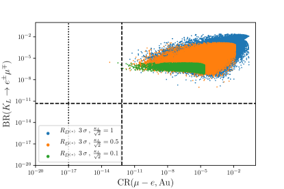
Figure 1: Associated predictions for CR($\mu-e$, Au) and BR($K_{L}\to e^{\pm}\mu^{\mp}$) for sample points satisfying $R_{D^{(\ast)}}$ at the $3\>\sigma$ level for the (unitary) parametrisation of Eq. (4). The dashed lines represent the current experimental upper bounds (see Tables 1 and 2 in Section 3.2), and the dotted line a benchmark future sensitivity to CR($\mu-e$, Al). All mixing angles have been varied randomly between $-\pi$ and $\pi$ and the leptoquark mass is set to $m_{V}\sim 1.5\mathrm{TeV}$. The blue, orange and green points respectively correspond to three benchmark choices, $\frac{\kappa_{L}}{\sqrt{2}}=1,\,0.5,\,0.1$.

2.2 Vector-like fermions and “effective” nonunitary mixings in the light sector

The above discussion suggests that the minimal flavour structure encoded in the (unitary) parametrisation of the leptoquark-quark-lepton currents (Eq. (3)) is insufficient to account for both anomalies. A stronger enhancement of LFUV in the leptoquark couplings can be achieved if one hypothesises that the “effective” leptoquark mixings - i.e. the $3\times 3$ matrix $V_{0}$ is nonunitary. As we proceed to discuss, in order to explain $R_{K^{(*)}}$ and $R_{D^{(*)}}$ data simultaneously, and for universal gauge couplings, a highly nonunitary flavour misalignment between quarks and leptons is in fact required.

Such a nonunitary flavour misalignment can be understood in the presence of heavy vector-like fermions, ${SU}(2)_{L}$ singlets or doublets, which have non-negligible mixings with the SM fermions. This can be encoded by generalising the charged lepton mixing matrix to a $3\times(3+n)$ semi-unitary matrix, so that SM interaction fields and physical states are related as $\ell^{0}_{L}=U^{\ell}_{L}\ell_{L}$ (for $n$ additional heavy states).

The Lagrangian of Eq. (3) can thus be recast as

$$\mathcal{L}\supset\sum_{i,j=1}^{3}\sum_{k=1}^{3+n}V_{1}^{\mu}\left(\bar{d}_{L}^{i}\gamma_{\mu}K_{L}^{ik}\ell_{L}^{k}+\bar{u}_{L}^{j}V^{\dagger}_{ji}\gamma_{\mu}K_{L}^{ik}U^{\text{P}}_{kj}\nu_{L}^{j}\right)+\text{H.c.}\,.$$ (5)

Notice that in the above equation, the effective leptoquark coupling $K_{L}$ generalises $K_{1}$ of Eq. (4), and now corresponds to a rectangular $3\times(3+n)$ matrix, which can be written in terms of $U_{L}^{\ell}$ as $K_{L}\equiv\frac{\kappa_{L}}{\sqrt{2}}U^{\ell}_{L}$.

Finally, $K_{L}$ can be further decomposed as $K_{L}=\left(K_{1},K_{2}\right)$, so that $K_{1}$ can be now identified with the nonunitary mixings in the light sectors (contrary to the simple limit of Eq. (4)). $K_{2}$ is a $3\times n$ matrix which corresponds to the $n$ heavy degrees of freedom describing the coupling parameters of the heavy (vector-like) states. Inspired by the approach frequently adopted in the context of neutrino physics, the deviation from unitarity in the $K_{1}$ block can now be parametrised as [116, 117, 118, 119]

$$K_{1}=\frac{\kappa_{L}}{\sqrt{2}}A\,V_{0}=\frac{\kappa_{L}}{\sqrt{2}}\begin{pmatrix}\alpha_{11}&0&0\\ \alpha_{21}&\alpha_{22}&0\\ \alpha_{31}&\alpha_{32}&\alpha_{33}\end{pmatrix}V_{0}\,,$$ (6)

with $V_{0}$ given in Eq. (4). The left-triangle matrix $A$, characterises the deviation from unitarity and encodes the effects of the mixings with the heavy states.

As already mentioned in the Introduction, we assume that the vector leptoquark $V_{1}$ appears as a gauge boson in an unspecified $SU(3)_{c}$ extension. Since neither the gauge embedding nor the Higgs sector is explicitly specified, our only assumption is that after EWSB all fermions (SM and vector-like) are massive, and that the physical eigenstates are obtained from the diagonalisation of an (effective) generic $(3+n)\times(3+n)$ lepton mass matrix. For simplicity (see Section 3.3), we take $n=3$ generations of heavy leptons in what follows; the $6\times 6$ charged lepton mass matrix $\mathcal{M}_{\ell}$ can be diagonalised by a bi-unitary transformation

$$\mathcal{M_{\ell}}^{\text{diag}}\,=\,U^{\ell\dagger}_{L}\,\mathcal{M_{\ell}}\,U^{\ell}_{R}\,.$$ (7)

Being a unitary $6\times 6$ matrix, $U^{\ell}_{L}$ can be parametrised by 15 real angles and 10 phases, and cast as a the product of 15 unitary rotations, $\mathcal{R}_{ij}$. By choosing a convenient ordering for the products of the complex rotation matrices, one can establish a parametrisation that allows isolating the information relative to the heavy leptons in a simple and compact form. Schematically, this can be described by the following ($2\times 2$ block matrix) decomposition [116], to which we adhere for the remainder of our discussion,

$$U^{\ell}_{L}=\begin{pmatrix}A&R\\ B&S\end{pmatrix}\begin{pmatrix}V_{0}&\mathbf{0}\\ \mathbf{0}&\mathbf{1}\end{pmatrix}$$ (8)

further defining

$$\begin{split}\begin{pmatrix}A&R\\ B&S\end{pmatrix}&=\mathcal{R}_{56}\mathcal{R}_{46}\mathcal{R}_{36}\mathcal{R}_{26}\mathcal{R}_{16}\mathcal{R}_{45}\mathcal{R}_{35}\mathcal{R}_{25}\mathcal{R}_{15}\mathcal{R}_{34}\mathcal{R}_{24}\mathcal{R}_{14}\>\text{,}\\ \begin{pmatrix}V_{0}&\mathbf{0}\\ \mathbf{0}&\mathbf{1}\end{pmatrix}&=\mathcal{R}_{23}\mathcal{R}_{13}\mathcal{R}_{12}\,.\end{split}$$ (9)

Under the above decomposition, one can still identify the SM-like mixings, given by $V_{0}$ (cf. Eq. (4)); the leptoquark couplings are now parametrised by the $3\times 6$ (rectangular) matrix,

$$K_{L}\,=\,(K_{1},K_{2})\,=\,\frac{\kappa_{L}}{\sqrt{2}}(A\,V_{0},R)\,.$$ (10)

The diagonal elements of the triangular matrix $A$, $\alpha_{ii}$, can be expressed as

$$\alpha_{ii}\,=\,c_{i6}\,c_{i5}\,c_{i4}\,,$$ (11)

in terms of the cosines of the mixing angles, ${c}_{ij}=\cos\theta_{ij}$. (The SM-like limit can be recovered for $A\to\mathbf{1}$.) The off-diagonal elements can be cast as [116]

$$\alpha_{21} = -c_{14}\,c_{15}\,\hat{s}_{16}\,\hat{s}^{\ast}_{26}-c_{14}\,\hat{s}_{15}\,\hat{s}^{\ast}_{25}\,c_{26}-\hat{s}_{14}\,\hat{s}^{\ast}_{24}\,c_{25}\,c_{26}\,,$$

$$\alpha_{32} = -c_{24}\,c_{25}\,\hat{s}_{26}\,\hat{s}^{\ast}_{36}-c_{24}\,\hat{s}_{25}\,\hat{s}^{\ast}_{35}\,c_{36}-\hat{s}_{24}\,\hat{s}^{\ast}_{34}\,c_{35}\,c_{36}\,,$$

$$\alpha_{31} = -c_{14}\,c_{15}\,\hat{s}_{16}\,c_{26}\,\hat{s}^{\ast}_{36}+c_{14}\,\hat{s}_{15}\,\hat{s}^{\ast}_{25}\,\hat{s}_{26}\,\hat{s}^{\ast}_{36}-c_{14}\,\hat{s}_{15}\,c_{25}\,\hat{s}^{\ast}_{35}\,c_{36}$$ (12)

$$+ \hat{s}_{14}\,\hat{s}^{\ast}_{24}\,c_{25}\,\hat{s}_{26}\,\hat{s}^{\ast}_{36}+\hat{s}_{14}\,\hat{s}^{\ast}_{24}\,\hat{s}_{25}\,\hat{s}^{\ast}_{35}\,c_{36}-\hat{s}_{14}\,c_{24}\,\hat{s}^{\ast}_{34}\,c_{35}c_{36}\,,$$

where $\hat{s}_{ij}\equiv e^{i\delta_{ij}}\sin\theta_{ij}$, with $\theta_{ij}$ and $\delta_{ij}$ respectively being the angles and CP phases associated with the $\mathcal{R}_{ij}$ rotation. Finally, it is worth emphasising that not only the full $6\times 6$ matrix $U_{L}^{\ell}$ is unitary, but its upper $3\times 6$ block $(AV_{0},R)$ is also semi-unitary on its own, with $\frac{2}{\kappa_{L}^{2}}K_{L}K_{L}^{\dagger}=1$.

This formalism, which can be easily generalised to $n$ extra generations, offers the possibility of successfully separating the information relative to the heavy leptons in a simple and compact form. Although the couplings (in particular the $\alpha_{ij}$ entries) can be in general complex, in what follows we consider a minimal scenario where all couplings are taken to be real.

3 Explaining LFUV data with nonunitary couplings: phenomenological viability

We recall that, as mentioned in the Introduction, we work under the minimal assumptions that the singlet vector leptoquark $V_{1}$ (colour triplet) should correspond to a gauge extension of $SU(3)_{c}$ unifying quarks and leptons with a universal (i.e., flavour independent) gauge coupling. We first describe the effects of the vector leptoquark on the neutral and charged current $b$ decays, and then summarise the most stringent constraints arising from numerous flavour violating and flavour conserving observables (meson oscillations and decays, as well as charged lepton flavour violation processes). We then present our main numerical results.

3.1 New contributions to $\boldsymbol{R_{K^{(\ast)}}}$ and $\boldsymbol{R_{D^{(\ast)}}}$

In what follows, we proceed to explore whether the relaxation of the unitarity requirement on the ${SU}(2)_{L}$-singlet vector leptoquark $V_{1}$ couplings to SM matter does allow addressing $R_{K^{(\ast)}}$ and $R_{D^{(\ast)}}$ data simultaneously.

Anomalies in neutral current $b$ decays: $\boldsymbol{R_{K^{(\ast)}}}$

As mentioned in the Introduction, several measurements of the ratio of branching ratios of $B\to K^{(*)}\ell\ell$ ($\ell=e,\mu$) exhibit tensions when compared to the SM predictions. The most recent averages (and SM estimations) are associated with the following deviations [11, 12, 13], in which the dilepton invariant mass squared bin (in $\text{GeV}^{2}$) is identified by the subscript:

$$R_{K[1.1,6]}^{\text{LHCb}}\, = \,0.846\,\pm_{0.054}^{0.060}\,\pm_{0.014}^{0.016}\,,\quad R_{K}^{\text{SM}}\,=\,1.0003\,\pm\,0.0001\,,$$

$$R_{K^{*}[0.045,1.1]}^{\text{LHCb}}\, = \,0.66^{+0.11}_{-0.07}\,\pm\,0.03\,,\quad R_{K^{*}[0.045,1.1]}^{\text{Belle}}\,=\,0.52^{+0.36}_{-0.26}\,\pm\,0.05\,,\quad R_{K^{*}[0.045,1.1]}^{\text{SM}}\,\sim\,0.93\,,$$

$$R_{K^{*}[1.1,6]}^{\text{LHCb}}\, = \,0.69^{+0.11}_{-0.07}\,\pm 0.05\,,\quad R_{K^{*}[1.1,6]}^{\text{Belle}}\,=\,0.96^{+0.45}_{-0.29}\,\pm 0.11\,,\quad R_{K^{*}[1.1,6]}^{\text{SM}}\,\sim\,0.99\,.$$ (13)

Other anomalies in the neutral current mode of $B$ meson decays have also emerged concerning the observable $\Phi\equiv d{\rm BR}(B_{s}\to\phi\mu\mu)/dm_{\mu\mu}^{2}$ in the analogous bin ($m_{\mu\mu}^{2}\in[1,6]\,{\rm GeV}^{2}$) [14], with a similar deviation (at a level of approximately $3\sigma$), as well as in the angular observable $P_{5}^{\prime}$ in $B\to K^{\ast}\ell^{+}\ell^{-}$ processes. While LHCb’s results for $P_{5}^{\prime}$ in $B\to K^{\ast}\mu^{+}\mu^{-}$ decays manifest a slight discrepancy with respect to the SM, the Belle Collaboration [15] reported that, when compared to the muon case, $P_{5}^{\prime}$ results for electrons show a better agreement with theoretical SM expectations. Nevertheless, there has been an ongoing discussion about the possibility that incorrectly estimated hadronic uncertainties might be at the origin of the observed anomalies in the mode $B\to K^{*}\mu^{+}\mu^{-}$, due to power corrections to the form factors, or charm-loop contributions [122, 123, 124, 125].

The effective Hamiltonian describing the neutral current effects at the level of quark transitions $d_{j}\to d_{i}\ell^{-}\ell^{\prime+}$ is given in Appendix A. A model-independent analysis of the current data at the $b$-quark mass scale can be made using the 2D hypothesis $C_{9,\text{NP}}^{\mu\mu}\,=-\,C_{10,\text{NP}}^{\mu\mu}$ and $C_{9,\text{NP}}^{ee}\,=-\,C_{10,\text{NP}}^{ee}$, allowing for the possibility of $(V-A)$ new physics (NP) effects in both electron and muon channels. Using the available experimental measurements of $R_{K^{(*)}}$ in different high and low $q^{2}$ bins, including the latest updates from LHCb and Belle collaborations, the available experimental measurements on the angular observables for $b\rightarrow s\mu\mu$ and $b\rightarrow see$, and the latest average for BR$(B_{s}\rightarrow\mu\mu)$ – which already includes the latest measurement from the ATLAS collaboration – we find the global fit ranges

$$-0.50\,(-0.58) \geq C_{9,sb}^{\mu\mu}=-C_{10,sb}^{\mu\mu} \geq(-0.83)\,-0.91\,,$$

$$0.00\,(-0.12) \geq C_{9,sb}^{ee}=-C_{10,sb}^{ee} \geq(-0.45)\,-0.55\,,$$ (14)

at the $2\,\sigma$ ($1\,\sigma$) level. In Fig. 2 we show the $1\sigma$ likelihood contours from the latest experimental measurements of $R_{K}^{(*)}$, $b\rightarrow s\mu\mu$ and $b\rightarrow see$ observables, as well as their combined global fit ($1\sigma$ and $2\sigma$) in the $C_{9,sb}^{\mu\mu}$ vs. $C_{9,sb}^{ee}$ plane, assuming the 2D hypothesis $C_{9,sb}^{\mu\mu}=-C_{10,sb}^{\mu\mu}$ and $C_{9,sb}^{ee}=-C_{10,sb}^{ee}$.

The vector leptoquark $V_{1}$ contributes at tree level, yielding the following Wilson coefficients at the leptoquark mass scale for the $\mathcal{O}_{9,10}^{ij;\ell\ell^{\prime}}$ operators [126]

$$C_{9}^{ij;\ell\ell^{\prime}}\,=\,-C_{10}^{ij;\ell\ell^{\prime}}\,=\,-\frac{\pi}{{\sqrt{2}{G_{F}}\,\alpha_{\text{em}}\,{V_{3j}}\,V_{3i}^{*}}}\,\frac{1}{{{m^{2}_{V}}}}K^{i\ell^{\prime}}_{L}\,K^{j\ell\ast}_{L}\,,$$ (15)

in which $G_{F}$ denotes the Fermi constant, $\alpha_{\text{em}}$ is the fine-structure constant, $V$ the CKM matrix, $K_{L}$ the “effective” leptoquark couplings (cf. Eq. (10)) and $m_{V}$ the vector leptoquark mass. The matching of the model parameters with the Wilson coefficients is performed at the scale of leptoquark mass and the Wilson coefficients are subsequently run down to the $b$-quark mass scale [115]. In particular, it is interesting to note that due to RG-running a large $K^{i\tau}_{L}$ coupling can potentially induce a non-negligible lepton-universal contribution to $b\to s\ell\ell$ transitions via a $\log$-enhanced anapole photon penguin contribution, as noted in Ref. [127]. The dominant $\log$-enhanced contribution is given by

$$\begin{aligned} \Delta C_{9}^{ij;\text{univ.}}&\approx-\sum_{\ell=e,\mu,\tau}\frac{\sqrt{2}}{G_{F}V_{tb}V_{ts}^{*}m^{2}_{V}}\,\frac{1}{6}\,K^{i\ell}_{L}\,K^{j\ell\ast}_{L}\,\log(m^{2}_{b}/m_{V}^{2})~{}.\end{aligned}$$ (16)

In our analysis, the running from the scale of leptoquark mass to the $b$-quark mass scale, and to any other relevant process (observable) scale, is taken into account using the wilson package [120] in association with the flavio package [121].

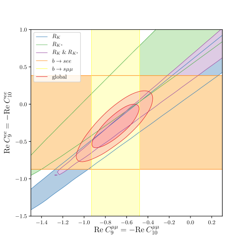
Figure 2: Likelihood $1\sigma$ contours from the latest measurements of $R_{K}^{(*)}$, $b\rightarrow s\mu\mu$, and $b\rightarrow see$ observables, as well as the combined global fit ($1\sigma$ and $2\sigma$) in the $C_{9,sb}^{\mu\mu}$ vs. $C_{9,sb}^{ee}$ plane, assuming the 2D hypothesis $C_{9,sb}^{\mu\mu}=-C_{10,sb}^{\mu\mu}$ and $C_{9,sb}^{ee}=-C_{10,sb}^{ee}$. The global fit is obtained at the $b$-quark mass scale using the package flavio [121].

Anomalies in charged current $b\to c\ell\bar{\nu}$ transitions: $\boldsymbol{R_{D^{(\ast)}}}$

Important deviations from the SM prediction of lepton flavour universality in $B\to D^{(*)}\ell\nu$ decays have also been reported by several experimental collaborations. The most recent averages for the $R_{D}$ and $R_{D^{(*)}}$ ratios by the HFLAV Collaboration [16] are

$$R_{D}\,=\,0.340\,\pm\,0.027\,\pm\,0.013\,,\quad R_{D}^{\text{SM}}\,=\,0.299\,\pm\,0.003\,\quad (1.4\sigma)\,;$$

$$R_{D^{*}}\,=\,0.295\,\pm\,0.011\,\pm\,0.008\,,\quad R_{D^{*}}^{\text{SM}}\,=\,0.258\,\pm\,0.005\,\quad (2.5\sigma)\,.$$ (17)

We define the effective Hamiltonian for the charged current transitions $d_{k}\to u_{j}\bar{\nu}\ell^{-}$ as

$$\mathcal{H}_{\text{eff}}^{\ell_{f}\nu_{i}}\,=\,\frac{4\,G_{F}}{\sqrt{2}}\,V_{jk}\,C_{jk}^{fi}\,\left(\bar{u}_{j}\,\gamma^{\mu}\,P_{L}\,d_{k}\right)\,\left({\bar{\ell}_{f}}\,\gamma_{\mu}\,P_{L}\,\nu_{i}\right)\,,$$ (18)

where, in the SM, $C_{jk,{\rm SM}}^{fi}=\delta_{fi}$. The contribution from the vector leptoquark $V_{1}$ is given by

$$C_{jk,V_{1}}^{fi}\,=\,\frac{\sqrt{2}}{4\,G_{F}\,m_{V}^{2}}\,\frac{1}{V_{jk}}\,(V\,K_{L}\,U^{P})_{ji}\,K_{L}^{kf\ast}\,.$$ (19)

One can further construct the double ratios

$$R_{D}/R_{D}^{\text{SM}}\,=\,R_{D^{\ast}}/R_{D^{\ast}}^{\text{SM}}\,=\,\sum_{i=1}^{3}\left|\delta_{3i}\,+\,C_{cb,V_{1}}^{\tau i}\right|^{2}\,,$$ (20)

(equal to unity when NP decouples, i.e., $\kappa_{L}\to 0$ and $m_{V}\to\infty$). After combining current experimental world averages with the SM predictions, the current anomalous data can be summarised as $R_{D}/R_{D}^{\text{SM}}\,=\,1.14\pm 0.10\,,\;R_{D^{\ast}}/R_{D^{\ast}}^{\text{SM}}\,=\,1.14\pm 0.06\,,$ in which the statistical and systematical errors have been added in quadrature. In Fig. 3, we display the $1\sigma$ and $2\sigma$ likelihood contours from $R_{K^{(*)}}$, $R_{D^{(*)}}$, $b\rightarrow s\mu\mu$ observables and the combined global fit ($1\sigma$, $2\sigma$ and $3\sigma$) in the plane $K_{L}^{33}K_{L}^{23}-K_{L}^{32}K_{L}^{22}$, where the couplings (see Eq. (3)) are varied independently and the others are set to zero.

As can be seen in Fig. 3, both $b\to c\ell\nu$ and $b\to s\ell\ell$ anomalies can be indeed accommodated simultaneously in a minimal $V_{1}$ model. However, we will subsequently show how this is realised in the nonunitary framework taking all couplings into account, as suggested by the $b\to s\ell\ell$ data.

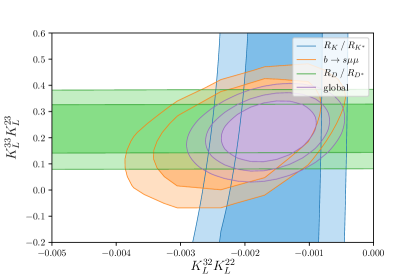
Figure 3: Likelihood $1\sigma$ and $2\sigma$ contours from $R_{K^{(*)}}$, $R_{D^{(*)}}$, $b\rightarrow s\mu\mu$ observables and the combined global fit ($1\sigma$, $2\sigma$ and $3\sigma$) in the plane $K_{L}^{33}K_{L}^{23}-K_{L}^{32}K_{L}^{22}$, defined at the leptoquark mass scale cf. Eq. (3). The first generation lepton and quark couplings are set to zero.

3.2 Constraints from (rare) flavour processes, EW precision observables and direct searches

The extended framework called upon to address the $B$ meson decay anomalies - not only the additional vector leptoquark, but also the presence of extra vector-like fermions, which are the origin of the nonunitarity of the $V_{1}$ effective couplings - opens the door to extensive contributions to numerous observables.

While most of the NP contributions occur via higher order (loop) exchanges, it is important to notice that $V_{1}$ can also mediate very rare (or even SM forbidden) processes already at the tree level. As we proceed to discuss, the latter observables prove to be particularly constraining, and put stringent bounds on the degrees of freedom of these leptoquark realisations.

Leptoquark SM extensions aiming at addressing the anomalies in $R_{K^{(\ast)}}$ and $R_{D^{(\ast)}}$ data receive strong constraints from $d_{j}\to d_{i}\bar{\nu}\nu$ transitions (in particular $s\to d\nu\nu$ and $b\to s\nu\nu$). However, the vector leptoquark $V_{1}$ does not generate contributions at tree level, and the first non-vanishing contribution appears at one loop. Consequently, we find that even with significant uncertainties, the semileptonic decays into charged dileptons $d_{j}\to d_{i}\ell^{-}\ell^{\prime+}$ often lead to tighter constraints (both the lepton flavour conserving and the lepton flavour violating modes). In the present analysis, we therefore include bounds from $K\to\pi\ell\ell^{\prime}$ and $B\to K\ell\ell^{\prime}$, as well as the stringent limits on NP contributions arising from the observed decay mode $B_{s}\to\mu^{+}\mu^{-}$. Furthermore, we also take into account the lepton flavour violating leptonic decays $B\to e^{\pm}\mu^{\mp}$, $B_{s}\to e^{\pm}\mu^{\mp}$ and $K_{L}\to e^{\pm}\mu^{\mp}$. Leptoquark contributions to neutral meson oscillations and mixings, such as $K^{0}-\bar{K}^{0}$ and $B_{s}^{0}-\bar{B}_{s}^{0}$, are also evaluated. Table 1 provides a brief summary of the current experimental status for these mesonic observables (current bounds and future sensitivities). A detailed discussion of the formalism used to evaluate the vector leptoquark contributions is provided in Appendix A.

Observables	SM prediction	Experimental data
$\text{BR}(K^{+}\to\pi^{+}\nu\bar{\nu})$	$(8.4\pm 1.0)\times 10^{-11}\phantom{|}{}^{\phantom{|}}_{\phantom{|}}$[128]	$17.3^{+11.5}_{-10.5}\times 10^{-11}\phantom{|}{}^{\phantom{|}}_{\phantom{|}}$[129] $<11\times 10^{-10}\phantom{|}{}^{\phantom{|}}_{\phantom{|}}$[130]
$\text{BR}(K_{L}\to\pi^{0}\nu\bar{\nu})$	$(3.4\pm 0.6)\times 10^{-11}\phantom{|}{}^{\phantom{|}}_{\phantom{|}}$[128]	$\leq 2.6\times 10^{-8}\phantom{|}{}^{\phantom{|}}_{\phantom{|}}$[131]
$R_{K^{(\ast)}}^{\nu\nu}$ ($B\to K^{(\ast)}\nu\bar{\nu}$)	$R_{K^{(\ast)}}^{\nu\nu}=1$	$R_{K}^{\nu\nu}<3.9$ $\phantom{a}{}^{\phantom{|}}_{\phantom{|}}$[132] $R_{K^{\ast}}^{\nu\nu}<2.7\phantom{|}^{\phantom{|}}_{\phantom{|}}$[132]
$B_{s}^{0}-\bar{B}_{s}^{0}$ (mixing parameters)	$\Delta_{s}=|\Delta_{s}|e^{i\phi_{s}}=1$ $\phantom{a}{}^{\phantom{|}}_{\phantom{|}}$ $\phi_{s}=0$	$|\Delta_{s}|=1.01^{+0.17}_{-0.10}\phantom{|}{}^{\phantom{|}}_{\phantom{|}}$[133], $\phi_{s}[^{\circ}]=1.3^{+2.3}_{-2.3}\phantom{|}{}^{\phantom{|}}_{\phantom{|}}$[133]
$K^{0}-\bar{K}^{0}$: $\Delta m_{K}/(10^{-15}\text{GeV})$	$3.1\pm 1.2\phantom{|}^{\phantom{|}}_{\phantom{|}}$[134]	$3.484\pm 0.006\phantom{|}^{\phantom{|}}_{\phantom{|}}$[1]
$\text{BR}(B_{s}\to\mu\mu)$	$(3.23\pm 0.27)\times 10^{-9}\phantom{|}{}^{\phantom{|}}_{\phantom{|}}$[135]	$2.7_{-0.5}^{+0.6}\times 10^{-9}\phantom{|}{}^{\phantom{|}}_{\phantom{|}}$[1]
$\text{BR}(K_{L}\to\mu^{\pm}e^{\mp})$	—	$<4.7\times 10^{-12}\phantom{|}{}^{\phantom{|}}_{\phantom{|}}$[1]
$\text{BR}(B_{s}\to\mu^{\pm}e^{\mp})$	—	$<1.1\times 10^{-8}\phantom{|}{}^{\phantom{|}}_{\phantom{|}}$[1]
$\text{BR}(B^{0}\to\mu^{\pm}e^{\mp})$	—	$<2.8\times 10^{-9}\phantom{|}{}^{\phantom{|}}_{\phantom{|}}$[1]
$\text{BR}(B^{0}\to\tau^{\pm}e^{\mp})$	—	$<2.8\times 10^{-5}\phantom{|}{}^{\phantom{|}}_{\phantom{|}}$[1]
$\text{BR}(B^{0}\to\tau^{\pm}\mu^{\mp})$	—	$<2.2\times 10^{-5}\phantom{|}{}^{\phantom{|}}_{\phantom{|}}$[1]
$\text{BR}(B^{0}\to K^{0}\mu^{\pm}e^{\mp})$	—	$<2.7\times 10^{-8}\phantom{|}{}^{\phantom{|}}_{\phantom{|}}$[1]
$\text{BR}(B^{0}\to\pi^{0}\mu^{\pm}e^{\mp})$	—	$<1.4\times 10^{-7}\phantom{|}{}^{\phantom{|}}_{\phantom{|}}$[1]
$\text{BR}(B^{\pm}\to K^{+}\mu^{\pm}e^{\mp})$	—	$<9.1\times 10^{-8}\phantom{|}{}^{\phantom{|}}_{\phantom{|}}$[1]
$\text{BR}(B^{\pm}\to K^{+}\tau^{\pm}e^{\mp})$	—	$<3.0\times 10^{-5}\phantom{|}{}^{\phantom{|}}_{\phantom{|}}$[1]
$\text{BR}(B^{\pm}\to K^{+}\tau^{\pm}\mu^{\mp})$	—	$<4.8\times 10^{-5}\phantom{|}{}^{\phantom{|}}_{\phantom{|}}$[1]
$\text{BR}(B^{\pm}\to\pi^{+}\mu^{\pm}e^{\mp})$	—	$<1.7\times 10^{-7}\phantom{|}{}^{\phantom{|}}_{\phantom{|}}$[1]
$\text{BR}(B^{\pm}\to\pi^{+}\tau^{\pm}e^{\mp})$	—	$<7.5\times 10^{-5}\phantom{|}{}^{\phantom{|}}_{\phantom{|}}$[1]
$\text{BR}(B^{\pm}\to\pi^{+}\tau^{\pm}\mu^{\mp})$	—	$<7.2\times 10^{-5}\phantom{|}{}^{\phantom{|}}_{\phantom{|}}$[1]

Table 1: Relevant observables and current experimental status for leptonic and semi-leptonic meson decays; when appropriate, the associated SM prediction is also included.

The lepton flavour non-universal couplings of vector leptoquarks (in general nonunitary in the present framework) induce new contributions to cLFV observables: radiative decays $\ell_{i}\rightarrow\ell_{j}\gamma$ and 3-body decays $\ell_{i}\rightarrow 3\ell_{j}$ at loop level, and neutrinoless $\mu-e$ conversion in nuclei both at tree and loop level. Further taking into account the impressive associated experimental sensitivity, it is clear that these observables lead to important constraints on the vector leptoquark couplings to SM fermions. It is important to stress that although the radiative decays are generated at higher order, relevant anapole contributions can add to the Wilson coefficients accounting for the tree-level contributions to neutrinoless $\mu-e$ conversion and $\mu\rightarrow 3e$. The higher order anapole contributions can have a magnitude comparable to the tree level ones (or even account for the dominant contribution). In addition, dipole operators also contribute significantly to radiative decays and to neutrinoless $\mu-e$ conversion. Although we do take tauonic modes into account, we notice here that due to the associated current experimental sensitivity, (semi)leptonic tau decays in general lead to comparatively looser constraints; likewise, semileptonic meson decays into final states including tau leptons are typically less constraining. However, the expected improvements in sensitivity from dedicated experiments might render the tau modes important probes of SM extensions via vector leptoquarks. As done for the first time in this work, all these contributions must be systematically included to thoroughly constrain the vector leptoquark couplings.

A summary of the current experimental status (current bounds and future sensitivities) is given in Table 2; for simplicity, in the numerical analysis we consider a benchmark future sensitivity to $\mu-e$ conversion in Aluminium of $\mathcal{O}(10^{-17})$. The relevant details of the computation of the cLFV observables considered in this work can be found in Appendix B.

cLFV process	Current experimental bound	Future sensitivity
$\text{BR}(\mu\to e\gamma)$	$4.2\times 10^{-13}$  (MEG [137])	$6\times 10^{-14}$  (MEG II [138])
$\text{BR}(\tau\to e\gamma)$	$3.3\times 10^{-8}$  (BaBar [139])	$10^{-9}$  (Belle II [140])
$\text{BR}(\tau\to\mu\gamma)$	$4.4\times 10^{-8}$  (BaBar [139])	$10^{-9}$  (Belle II [140])
$\text{BR}(\mu\to 3e)$	$1.0\times 10^{-12}$  (SINDRUM [141])	$10^{-15(-16)}$  (Mu3e [142])
$\text{BR}(\tau\to 3e)$	$2.7\times 10^{-8}$  (Belle [143])	$10^{-9}$  (Belle II [140])
$\text{BR}(\tau\to 3\mu)$	$3.3\times 10^{-8}$  (Belle [143])	$10^{-9}$  (Belle II [140])
$\text{CR}(\mu-e,\text{N})$	$7\times 10^{-13}$  (Au, SINDRUM [144])	$10^{-14}$  (SiC, DeeMe [145])
		$7\times 10^{-15}(3\times 10^{-18})$  (Al, COMET [146, 147])
		$8\times 10^{-17}$  (Al, Mu2e [148])

Table 2: Current experimental bounds and future sensitivities of various cLFV processes considered in the analysis.

The presence of heavy vector-like fermions (at the source of the nonunitary couplings of the vector leptoquark to the light fermions) can have a non-negligible impact on the couplings of SM fermions to gauge bosons. In turn, this can be manifest in new contributions to several EW precision observables - potentially in conflict with SM expectations and precision data -, which will prove to play a key role in constraining the mixings of the SM charged leptons with the heavy states.

For the $Z$-couplings, which are modified at the tree level, the most stringent constraints are expected to arise from leptonic $Z$ decays; in our analysis, we take into account the LFU ratios and cLFV decay modes of the $Z$ boson. We summarise in Table 3 the EWP observables which are of relevance for our study (experimental measurements and SM predictions). A discussion on how the $\bar{f}fZ$ couplings are modified as a consequence of nonunitary effective leptoquark couplings, as well as their impact for several observables, is detailed in Appendix C.

Observables	Experimental data	SM Prediction
$\Gamma_{Z}$	$2.4952\pm 0.0023\>\mathrm{GeV}$	$2.4942\pm 0.0008\>\mathrm{GeV}$
$\Gamma(Z\to\ell^{+}\ell^{-})$	$83.984\pm 0.086\>\mathrm{MeV}$	$83.959\pm 0.008\>\mathrm{MeV}$
$R_{e}$	$20.804\pm 0.050$	$20.737\pm 0.010$
$R_{\mu}$	$20.785\pm 0.033$	$20.737\pm 0.010$
$R_{\tau}$	$20.764\pm 0.045$	$20.782\pm 0.010$
$\mathrm{BR}(Z\to e^{\pm}\mu^{\mp})$	$<7.5\times 10^{-7}$	–
$\mathrm{BR}(Z\to e^{\pm}\tau^{\mp})$	$<9.8\times 10^{-6}$	–
$\mathrm{BR}(Z\to\mu^{\pm}\tau^{\mp})$	$<1.2\times 10^{-5}$	–

Table 3: Subset of EWP observables affected by the modified $Z$ couplings, with the corresponding experimental measurements and SM predictions [1]. The ratios $R_{\ell}$ are defined as $R_{\ell}={\Gamma_{\text{had}}}/{\Gamma(Z\to\ell^{+}\ell^{-})}$, and $\Gamma(Z\to\ell^{+}\ell^{-})$ denotes an average over $\ell=e,\,\mu,\,\tau$.

Finally, it is clear that the (negative) results of direct searches for the exotic states must be taken into account. At the LHC, pairs of vector leptoquarks can be abundantly produced in various processes (via $t$-channel lepton exchange and direct couplings to one or two gluons). Due to the underlying gauge structure of possible ultraviolet (UV) completions, the production cross section strongly depends on the coupling to gluons which makes the theoretical predictions for the production of vector leptoquarks less robust than those for scalar leptoquarks. On the other hand, if the vector leptoquark corresponds to a spontaneously broken non-abelian gauge symmetry, gauge invariance completely fixes the couplings between the vector leptoquark and the gluons, implying lower limits on the vector leptoquark mass (albeit still depending on the branching fractions of the leptoquark) from the negative results in the direct searches for pair production at the LHC, see for instance [102]. As a natural consequence of the favoured structure called upon to maximise the effects on $B$-meson decay anomalies, $V_{1}$ is expected to dominantly decay into either $t\bar{\nu}_{\tau}$ or $b\bar{\tau}$. The ATLAS and CMS collaborations have conducted extensive searches, assuming that leptoquarks couple exclusively to third generation quarks and leptons [150, 151, 152, 153, 154], which have led to lower limits on the $V_{1}$ mass $\sim 1.5$ TeV. Further important collider signatures are $pp\to\tau\bar{\tau}+X$, arising from $t$-channel leptoquark exchange or from single leptoquark production in association with a charged lepton. As argued in [155, 156], the projected vector leptoquark reach of HL-LHC with $3$ ab^-1 is close to $1.8$ TeV. Much higher luminosities and/or more sophisticated search strategies are required to probe the preferred mass scale and couplings of states at the origin of a combined explanation of the anomalies (for instance, as suggested by the study of [96]). Other potentially interesting search modes could include $b\mu b\tau$ and $b\mu b\mu$ final states.

In the present analysis, we select (working) benchmark values for the mass and gauge coupling of the vector leptoquark allowing to comply with the current available limits. In particular, for the following numerical analysis we set $\frac{\kappa_{L}}{\sqrt{2}}=1$ as a benchmark choice. Nevertheless, for any other choice consistent with the constraints from direct searches (as discussed above) the qualitative behaviour and the conclusions drawn remain the same. However, for very small values $\kappa_{L}$ ($\kappa_{L}\lesssim 0.1$ for $m_{V}\gtrsim 1.5$ TeV) the number of points in the best fit region for $R_{K^{(*)}}$ and $R_{D^{(*)}}$ anomalies starts to decrease drastically, so that the NP effects become negligible with respect to the SM.

3.3 Results and discussion

We now finally address the question of whether a SM extension via vector leptoquarks can simultaneously provide an explanation to both the $R_{K^{(\ast)}}$ and $R_{D^{(\ast)}}$ data, working under the hypothesis of universal gauge couplings for the vector leptoquark $V_{1}$. In this framework, the required flavour non-universality arises from nonunitary mixings among the SM fermions - a consequence of the existence of heavy vector-like fermions which have non-negligible mixings with the light fields.

We first begin by considering the most minimal scenario where the nonunitary flavour misalignment is due to the presence of a single generation of heavy vector-like charged leptons (i.e., $n=1$ in Eq. (5)). Such a minimal field content already leads to a sufficient amount of LFUV to account for both $R_{K^{(*)}}$ and $R_{D^{(*)}}$ anomalies. Although new contributions to rare meson decays and transitions are still in good agreement with current experimental bounds, this scenario is ruled out due to the stringent constraints on cLFV modes. Excessive contributions to (tree-level) muon-electron conversion in nuclei play a crucial role in ruling out this realisation, as well as the closely related radiative decays. In order to reconcile the model’s prediction with the current bounds on CR($\mu-e$, Au), the photon-penguin contributions must (at least) partially cancel the sizeable tree-level ones; however, such large photon-penguin contributions then translate into unacceptably large $\mu\to e\gamma$ decay rates, already in conflict with current bounds.

The required flavour non-universality can be recovered for a less dramatic unitarity violation; this can be achieved by extending the particle content by two or more additional heavy charged lepton states, or formally for $n\geq 2$ in Eq. (5). Although $n=2$ provides more freedom to evade the constraints found in the case $n=1$, no generic solution was found in this case, which might then require an extreme fine tuning to become viable. In the subsequent discussion, we therefore take $n=3$ which is the minimal case and conveniently replicates the number of generations in the SM.

For $n=3$, our study suggests that it is in general possible to find regions in the parameter space in which the required non-universal flavour structure to explain both $R_{K^{(*)}}$ and $R_{D^{(*)}}$ arises in a natural way, while still complying with all constraints from flavour violating processes (meson and lepton sectors). This can be seen from the upper row of Fig. 4, in which we display the regimes for the entries of the matrix $A$ (cf. Eqs. (8) - (2.2)) which account for both $R_{K^{(*)}}$ and $R_{D^{(*)}}$ data, as well as regions respecting the constraints arising from the several flavour violating modes considered in our analysis. Concerning the latter, we find it worth mentioning that the most stringent constraints arise from $K_{L}\to\mu^{\pm}e^{\mp}$, $\mu\to e\gamma$, and $\mu-e$ conversion in nuclei; $B$-meson cLFV decays, or (semi)leptonic $B$ and $K$ decays lead to comparatively milder constraints (or are systematically satisfied).

         

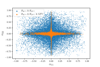
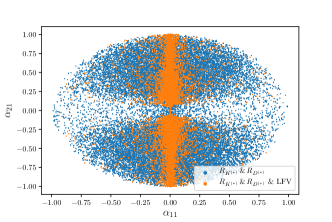
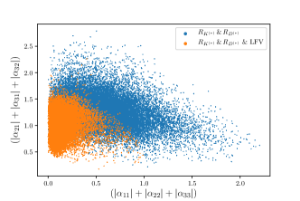
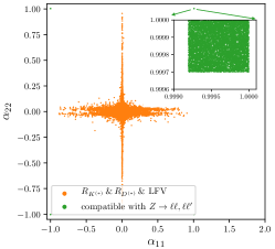
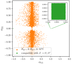
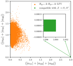
Figure 4: On the upper row, $A$-matrix entries complying with $R_{K^{(*)}}$ and $R_{D^{(*)}}$ data (blue) and those which in addition respect all imposed flavour constraints (yellow). Lower row: for the case of isosinglet heavy leptons, $A$-matrix entries complying with $R_{K^{(*)}}$ and $R_{D^{(*)}}$ data as well as LFV bounds (yellow), and those which now further comply with bounds from $Z$ decays (green). (Notice that the green inset area corresponds to a zoom-out of what would otherwise be a tiny region close to the border of the parameter space.) In all panels we have taken $m_{V}=1.5$ TeV and all mixing angles have been varied randomly between $-\pi$ and $\pi$.

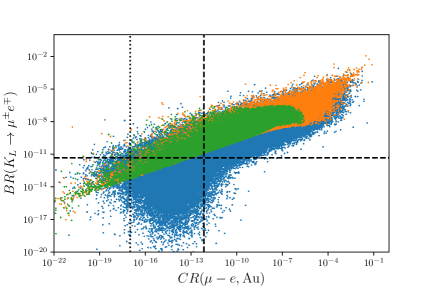
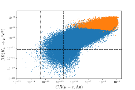
Figure 5: Regions in the plane spanned by CR($\mu-e$,N) and BR($K_{L}\to\mu^{\pm}e^{\mp}$), accommodating $R_{K^{(*)}}$ (left panel) and $R_{D^{(*)}}$ (right panel), respectively for leptoquark masses in the intervals $m_{V}\in[15~{}\text{TeV},45~{}\text{TeV}]$ and $m_{V}\in[1~{}\text{TeV},6~{}\text{TeV}]$, in the framework of nonunitary leptoquark couplings induced by the presence of 3 generations of isosinglet heavy leptons. Blue points satisfy $R_{{K^{(*)}},\,{D^{(*)}}}$ at the 3 $\sigma$ level, yellow points are consistent with leptonic $Z$ decays, and green points are compatible with all imposed constraints, other than those depicted by the corresponding vertical and horizontal dashed lines (dotted ones denoting future sensitivities). In both panels, all mixing angles have been varied randomly between $-\pi$ and $\pi$.

Finally, one should address the compatibility of the considered SM leptoquark extension with the constraints arising from EW precision tests; as discussed in the previous subsection (and in Appendix C), nonunitary mixings can modify the couplings of the $Z$ boson. In particular, for isosinglet heavy leptons, the entries of the matrix $A$ (see Eqs. (11) and (2.2)) are severely constrained by the $Z$ width and by bounds on its cLFV decays ($Z\to\ell\ell^{\prime}$). This is shown on the lower row of Fig. 4, which illustrates the tension between LFUV and $Z$ bounds - a tension which ultimately leads to disfavouring this class of extensions as a phenomenologically viable NP model to explain both $R_{K^{(*)}}$ and $R_{D^{(*)}}$ discrepancies.

If one foregoes a solution to the charged current anomalies (i.e., $R_{D^{(*)}}$), it is possible to accommodate $R_{K^{(*)}}$ in full agreement with constraints from flavour bounds, relying on very mild deviations from unitarity, and thus evading constraints from universality violation in $Z$ decays. However, one would be led to regions with considerably heavier leptoquarks, $m_{V}\gtrsim 15$ TeV. This is depicted on the left panel of Fig. 5, in which we display regimes complying with $R_{K^{(*)}}$ at the $3\sigma$ level) in the plane spanned by two particularly constraining observables, BR($K_{L}\to\mu^{\pm}e^{\mp}$) and CR($\mu-e$, N), for $15\text{ TeV}\lesssim m_{V}\lesssim 45\text{ TeV}$. As can be verified, a small subset of points (consistent with $R_{K^{(*)}}$ and respecting universality in $Z$ decays) is compatible with current bounds on the cLFV processes. This is in agreement with the analyses of various UV-complete models, such as [103, 104].

For completeness, the right panel of Fig. 5 shows a similar study for $R_{D^{(*)}}$. In order to accommodate $R_{D^{(*)}}$ data, lower leptoquark masses are required (in this case we have taken $1\text{ TeV}\lesssim m_{V}\lesssim 6\text{ TeV}$), and it is no longer possible to evade $K_{L}\to\mu^{\pm}e^{\mp}$ and $\mu-e$ conversion bounds while being consistent with leptonic $Z$-decay universality. The data displayed in the panels of Fig. 4 was obtained for vector leptoquark masses $m_{V}\sim 1.5$ TeV; analogous conclusions can be inferred for $m_{V}\sim\mathcal{(}1-3)$ TeV, albeit for different $\alpha_{ij}$ ranges.

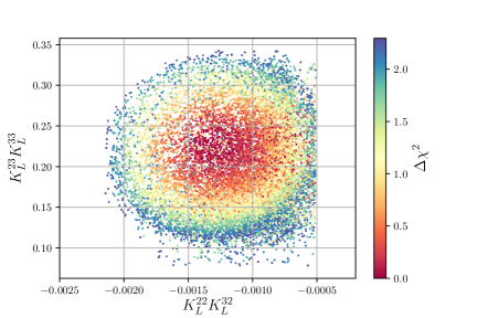
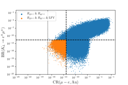
Figure 6: On the left, $\Delta\chi^{2}$ distribution for the fit to $R_{K^{(*)}}$ and $R_{D^{(*)}}$ data ($1\sigma$) in the plane of the $(K_{L})_{ij}$ couplings. All points comply with the different (flavour) constraints. On the right, regions in the plane spanned by CR($\mu-e$,N) and BR($K_{L}\to\mu^{\pm}e^{\mp}$), accommodating both $R_{K^{(*)}}$ and $R_{D^{(*)}}$ (blue) and those in addition complying with LFV constraints (yellow). Both panels correspond to a heavy sector composed of three isodoublet vector-like charged lepton states, and to having set $m_{V}\sim 1.5$ TeV. The $\mathrm{\Delta}\chi^{2}$ corresponds to the $1\,\sigma$-region around the best fit point.

Since for the case of isosinglet leptons an explanation of $R_{D^{(*)}}$ is excluded by bounds on $Z$ decays, we now consider isodoublet heavy charged leptons. The nonunitarity in the couplings of the vector leptoquark to the SM charged leptons can simultaneously explain $R_{K^{(*)}}$ and $R_{D^{(*)}}$ data. Moreover, and by construction, in the case of isodoublet heavy charged lepton states $Z\ell\ell$ couplings remain universal (in the absence of mixings between right-handed SM charged leptons and vector-like doublets, $\Delta g_{R}=0$, see Appendix C); nevertheless, flavour observables still play a crucial role, and are (as expected) responsible for severe constraints on the NP degrees of freedom.

The left panel of Fig. 6 offers a global view of this case, showing the $\Delta\chi^{2}$ distribution for the fit to $R_{K^{(*)}}$ and $R_{D^{(*)}}$ data, in the plane spanned by $(K_{L})_{ij}$ “muon and tau couplings” ($K_{22}K_{32}-K_{23}K_{33}$), marginalising over the other couplings. The leptoquark mass is set to $m_{V}\sim 1.5$ TeV. We stress that leading to this plot all couplings were determined by the underlying nonunitarity parametrisation (with all mixing angles randomly sampled); in particular, we have not set the leptoquark couplings to the first generation of quark and leptons to zero. The displayed points comply with all flavour bounds included in our study, as described in Section 3.2.

The lowest $\Delta\chi^{2}$ region (dark red ellipsoid) suggests that the best fit scenario corresponds to new physics dominantly coupling to muons and taus. We stress that the patterns emerging from the $\Delta\chi^{2}$ distribution are not an artefact of some particular assumption imposed on the couplings, but rather the result of a very general scan over the full set of (mixing) parameters.

The right panel of Fig. 6 offers a projection of the viable points (displayed on the left panel) in the plane of the most constraining observables, CR($\mu-e$,N) and BR($K_{L}\to\mu^{\pm}e^{\mp}$). It is interesting to notice that, to a very good approximation, most of the currently phenomenologically viable points lie within future reach of the upcoming muon-electron conversion dedicated facilities (COMET and Mu2e).

In the near future, and should the $B$-meson decay anomalies be confirmed, an explanation in terms of such a minimal leptoquark framework could be probed via its impact for cLFV observables, in particular $\mu-e$ conversion in nuclei. Although the cLFV bounds could be evaded by increasing the mass of the vector leptoquark, this would however prevent a viable explanation of the $B$-meson decay anomalies, especially of $R_{D^{(*)}}$.

4 Concluding remarks

In this study we have considered a minimal SM extension via one vector leptoquark $V_{1}$ and $n$ generations of heavy vector-like charged leptons, as a candidate framework to explain the current $B$-meson anomalies, $R_{K^{(*)}}$ and $R_{D^{(*)}}$.

Minimal extensions by a single $V_{1}$ leptoquark are in general disfavoured due to the strong cLFV constraints on the (unitary) quark-lepton-$V_{1}$ couplings. Here we have suggested that the pattern of mixings required to simultaneously address $R_{K^{(*)}}$ and $R_{D^{(*)}}$ with a single $V_{1}$ could be interpreted within a framework of nonunitary $V_{1}\ell q$ couplings: the mixings of the SM charged leptons with the additional vector-like heavy leptons can lead to effectively nonunitary $V_{1}\ell q$ couplings, offering the required amount of LFUV to account for both anomalies.

As we have argued, the most minimal nonunitary scenario (i.e. $n=1$) consistent with both $R_{K^{(*)}}$ and $R_{D^{(*)}}$, is ruled out as it leads to excessive contributions to cLFV observables such as muon-electron conversion in nuclei. We have thus considered three families of vector-like heavy leptons, and we have carried out a detailed analysis of the impact for an extensive array of flavour violation and EW precision observables. Our findings revealed that the $SU(2)_{L}$ charges of the heavy charged leptons are of paramount importance for the model’s viability: for isosinglet heavy leptons, the mass of the leptoquark must be sufficiently large to avoid excessive contributions to $Z$ decays, which then prevents an explanation of $R_{D^{(*)}}$. This is expected to happen for heavy leptons of any $SU(2)_{L}$ representation except for isodoublets. In this particular case, the $Z\ell\ell$ couplings remain universal, and we have shown that the nonunitarity in the couplings allows to successfully explain both sets of anomalies, while complying with all considered current bounds.

The nonunitary framework here considered in fact provides one of the most economical options to simultaneously address $R_{K^{(\ast)}}$ and $R_{D^{(\ast)}}$ data via a single vector leptoquark. Although our results arise from a phenomenological analysis, our findings can be easily related to well-motivated UV complete models, in which the nonunitarity framework allows to obtain the required flavour structure without further enlarging the gauge group. Interestingly, this is the case of the Pati-Salam model [97, 98, 99, 100, 101, 102, 103, 104, 105, 106], in which the existence of a vector leptoquark with a mass around the TeV scale (as required for a successful simultaneous explanation of both the neutral and charged current anomalies) naturally motivates the existence of such vector-like heavy leptons.

Finally, it is worth stressing that in view of the important progress expected in the near future, cLFV searches can play a crucial role in falsifying these minimal leptoquark frameworks, in view of their strong impact for cLFV observables, in particular $\mu-e$ conversion in nuclei. As we have discussed, should the $B$-meson decay anomalies be verified, and should this be a valid framework to explain them, then one should expect the observation of cLFV signals, in particular from $\mu-e$ conversion in Aluminium targets, either at COMET or Mu2e.

Appendix A Constraints from flavour violating rare meson decays and neutral meson mixing

New physics frameworks including leptoquarks give rise to important contributions to observables in the meson sector. These include flavour conserving and flavour violating leptonic and semileptonic decays (including final state neutrinos), as well as neutral meson mixings. In this appendix we discuss the different leptoquark contributions to leptonic and semi-leptonic meson decays (arising at tree-level) and to modes with final state neutrinos (at one-loop level). We recall that the SM predictions and current experimental limits are summarised in Table 1.

Note that the matching of the model’s parameters with the Wilson coefficients is performed at the scale of the leptoquark mass, and then these are run down to the $b$-quark mass scale. In our analysis, the running from the scale of leptoquark mass to the $b$-quark mass scale, and to any other relevant process (observable) scale, is taken into account using the wilson package [120] in association with the flavio package [121].

A.1 Exclusive $d_{j}\rightarrow d_{i}\ell^{-}\ell^{\prime+}$ decays

The effective Hamiltonian for $d_{j}\rightarrow d_{i}\ell^{-}\ell^{\prime+}$ transitions, including the LFV operators, can be cast as [157, 158, 159, 160, 161, 162]

$$\mathcal{H}_{\text{eff}}=-\frac{4G_{F}}{\sqrt{2}}V_{3j}V_{3i}^{\ast}\Big{[}\sum_{\begin{array}[]{c}k=7,9,\\ 10,S,P\end{array}}\left(C_{k}(\mu)\mathcal{O}_{k}(\mu)+C_{k}^{{}^{\prime}}(\mu)\mathcal{O}_{k}^{{}^{\prime}}(\mu)\right)+C_{T}(\mu)\mathcal{O}_{T}(\mu)+C_{T_{5}}(\mu)\mathcal{O}_{T_{5}}(\mu)\Big{]}.$$ (21)

In the above, we recall that $V_{ij}$ denotes the CKM matrix; the operators are defined as

$$\mathcal{O}_{7}^{ij} =\frac{em_{d_{j}}}{(4\pi)^{2}}(\bar{d}_{i}\sigma_{\mu\nu}P_{R}d_{j})F^{\mu\nu}\>\text{,}$$

$$\mathcal{O}_{9}^{ij;\ell\ell^{\prime}} =\frac{e^{2}}{(4\pi)^{2}}(\bar{d}_{i}\gamma^{\mu}P_{L}d_{j})(\bar{\ell}\gamma_{\mu}\ell^{\prime})\>\text{,}$$

$$\mathcal{O}_{10}^{ij;\ell\ell^{\prime}} =\frac{e^{2}}{(4\pi)^{2}}(\bar{d}_{i}\gamma^{\mu}P_{L}d_{j})(\bar{\ell}\gamma_{\mu}\gamma_{5}\ell^{\prime})\>\text{,}$$

$$\mathcal{O}_{S}^{ij;\ell\ell^{\prime}} =\frac{e^{2}}{(4\pi)^{2}}(\bar{d}_{i}P_{R}d_{j})(\bar{\ell}\ell^{\prime})\>\text{,}$$

$$\mathcal{O}_{P}^{ij;\ell\ell^{\prime}} =\frac{e^{2}}{(4\pi)^{2}}(\bar{d}_{i}P_{R}d_{j})(\bar{\ell}\gamma_{5}\ell^{\prime})\>\text{,}$$

$$\mathcal{O}_{T}^{ij;\ell\ell^{\prime}} =\frac{e^{2}}{(4\pi)^{2}}(\bar{d}_{i}\sigma_{\mu\nu}d_{j})(\bar{\ell}\sigma^{\mu\nu}\ell^{\prime})\>\text{,}$$

$$\mathcal{O}_{T5}^{ij;\ell\ell^{\prime}} =\frac{e^{2}}{(4\pi)^{2}}(\bar{d}_{i}\sigma_{\mu\nu}d_{j})(\bar{\ell}\sigma^{\mu\nu}\gamma_{5}\ell^{\prime})\>\text{,}$$ (22)

with the primed operators $\mathcal{O}_{7,9,10,S,P}^{\prime}$ following from the replacement $P_{L}\leftrightarrow P_{R}$.

Regarding lepton flavour violating processes, only the operators $\mathcal{O}_{9,10,S,P}^{(\prime)}$ play a relevant role: for vector leptoquarks, the complete set of associated Wilson coefficients (not present in the SM) is given by [126]

$$C^{ij;\ell\ell^{\prime}}_{9,10} =\mp\frac{\pi}{\sqrt{2}G_{F}\,\alpha_{\text{em}}\,V_{3j}\,V_{3i}^{\ast}\,m_{V}^{2}}\left(K_{L}^{i\ell^{\prime}}\,K_{L}^{j\ell\ast}\right)$$

$$C^{\,\prime\,ij;\ell\ell^{\prime}}_{9,10} =-\frac{\pi}{\sqrt{2}G_{F}\,\alpha_{\text{em}}\,V_{3j}\,V_{3i}^{\ast}\,m_{V}^{2}}\left(K_{R}^{i\ell^{\prime}}\,K_{R}^{j\ell\ast}\right)$$

$$C^{ij;\ell\ell^{\prime}}_{S,P} =\pm\frac{\pi}{\sqrt{2}G_{F}\,\alpha_{\text{em}}\,V_{3j}\,V_{3i}^{\ast}\,m_{V}^{2}}\left(K_{L}^{i\ell^{\prime}}\,K_{R}^{j\ell\ast}\right)$$

$$C^{\,\prime\,ij;\ell\ell^{\prime}}_{S,P} =\frac{\pi}{\sqrt{2}G_{F}\,\alpha_{\text{em}}\,V_{3j}\,V_{3i}^{\ast}\,m_{V}^{2}}\left(K_{R}^{i\ell^{\prime}}\,K_{L}^{j\ell\ast}\right)\>\text{,}$$ (23)

where $K_{L}^{i\ell}$ ($K_{R}^{i\ell}$) denoting the left-handed (right-handed) leptoquark couplings. Here, and for completeness, we include the $K_{R}$ mixing matrix, although we do not take it into account in our analysis.

A.2 $P\rightarrow\ell^{-}\ell^{\prime+}$ decays

Leptonic decays of pseudoscalar mesons lead to important constraints on the (vector) leptoquark couplings. Here, we summarise the computation of the $P\rightarrow\ell^{-}\ell^{\prime+}$ rates, following the derivation of [163]. With the standard decomposition of the hadronic matrix element

$$\langle 0\,|\,\bar{d}_{j}\,\gamma_{\mu}\,\gamma_{5}\,d_{i}|\,P(p)\rangle\,=\,i\,p_{\mu}\,f_{P}\,,$$ (24)

in which $f_{P}$ denotes the $P$ meson decay constant, the branching fraction is given by

$$\text{BR}(P \rightarrow\ell^{-}\,\ell^{\prime+})\,=\,\frac{\tau_{P}}{64\,\pi^{3}}\frac{\alpha^{2}\,G_{F}^{2}}{m_{P}^{3}}\,f_{P}^{2}\,|V_{3j}\,V_{3i}^{{\ast}}|^{2}\,\lambda^{\frac{1}{2}}(m_{P},m_{\ell},m_{\ell^{\prime}})$$

$$\times\Bigg{\{}\left(m_{P}^{2}-\left(m_{\ell}+m_{\ell^{\prime}}\right)^{2}\right)\Bigg{|}\left(C_{9}-C_{9}^{\prime}\right)\left(m_{\ell}-m_{\ell^{\prime}}\right)+\left(C_{S}-C_{S}^{\prime}\right)\frac{m_{P}^{2}}{m_{d_{j}}+m_{d_{i}}}\Bigg{|}^{2}$$

$$+\left(m_{P}^{2}-\left(m_{\ell}-m_{\ell^{\prime}}\right)^{2}\right)\Bigg{|}\left(C_{10}-C_{10}^{\prime}\right)\left(m_{\ell}+m_{\ell^{\prime}}\right)+\left(C_{P}-C_{P}^{\prime}\right)\frac{m_{P}^{2}}{m_{d_{j}}+m_{d_{i}}}\Bigg{|}^{2}\Bigg{\}}\,,$$ (25)

where the Källén-function is defined as

$$\lambda(a,b,c)=\left(a^{2}-\left(b-c\right)^{2}\right)\left(a^{2}-\left(b+c\right)^{2}\right)\,\text{.}$$ (26)

Since this FCNC transition is generated at tree-level from $V_{1}$ interactions, the modes leading to different final state lepton charge assignments must both be included and treated separately. Leptonic pseudoscalar meson decays thus provide extensive (and very tight) constraints on the leptoquark couplings.

A.3 $P\rightarrow P^{\prime}\ell^{-}\ell^{\prime+}$ decays

Again working in the standard basis, the hadronic matrix elements are parametrised as

$$\langle\bar{P}^{\prime}(k)\,|\,\bar{d}_{i}\,\gamma_{\mu}\,d_{j}\,|\,\bar{P}(p)\rangle=\left[(p+k)_{\mu}-\frac{m_{P}^{2}-m_{P^{\prime}}^{2}}{q^{2}}q_{\mu}\right]\,f_{+}(q^{2})+\frac{m_{P}^{2}-m_{P^{\prime}}^{2}}{q^{2}}q_{\mu}\,f_{0}(q^{2})\,,$$ (27)

$$\langle\bar{P}^{\prime}(k)\,|\,\bar{d}_{i}\,\sigma_{\mu\nu}\,d_{j}\,|\,\bar{P}(p)\rangle=-i\,\left(p_{\mu}\,k_{\nu}-p_{\nu}\,k_{\mu}\right)\frac{2}{m_{P}+m_{P^{\prime}}}\,f_{T}(q^{2},\mu)\,.$$ (28)

In the above, the hadronic form factors $f_{+,0,T}(q^{2})$ depend on the momentum transfer, which lies in the range $(m_{\ell}+m_{\ell^{\prime}})^{2}\leq q^{2}\leq(m_{P}-m_{P^{\prime}})^{2}$. In our evaluation of the form factors we closely follow the results of [164]; since we focus on decays with heavy-to-light meson transitions, we further assume the scale to be $\mu=m_{d_{j}}$, i.e. $\mu=m_{b}$. With the quantities

$$\varphi_{7}(q^{2}) =\frac{2\,m_{d_{j}}\,|f_{T}(q^{2})|^{2}}{(m_{P}+m_{P^{\prime}})^{2}}\,\lambda(m_{P},m_{P^{\prime}},\sqrt{q^{2}})\,\left[1-\frac{(m_{\ell}-m_{\ell^{\prime}})^{2}}{q^{2}}-\frac{\lambda(\sqrt{q^{2}},m_{\ell},m_{\ell^{\prime}})}{3\,q^{4}}\right]\>\text{,}$$

$$\varphi_{9(10)}(q^{2}) =\frac{1}{2}\,|f_{0}(q^{2})|^{2}(m_{\ell}\mp m_{\ell^{\prime}})^{2}\,\frac{(m_{P}^{2}-m_{P^{\prime}}^{2})^{2}}{q^{2}}\,\left[1-\frac{(m_{\ell}\pm m_{\ell^{\prime}})^{2}}{q^{2}}\right]$$

$$+\frac{1}{2}\,|f_{+}(q^{2})|^{2}\,\lambda(m_{P},m_{P^{\prime}},\sqrt{q^{2}})\,\left[1-\frac{(m_{\ell}\mp m_{\ell^{\prime}})^{2}}{q^{2}}-\frac{\lambda(\sqrt{q^{2}},m_{\ell},m_{\ell^{\prime}})}{3\,q^{4}}\right]\>\text{,}$$

$$\varphi_{79}(q^{2}) =\frac{2\,m_{d_{j}}\,f_{+}(q^{2})\,f_{T}(q^{2})}{m_{P}+m_{P^{\prime}}}\,\lambda(m_{P},m_{P^{\prime}},\sqrt{q^{2}})\,\left[1-\frac{(m_{\ell}-m_{\ell^{\prime}})^{2}}{q^{2}}-\frac{\lambda(\sqrt{q^{2}},m_{\ell},m_{\ell^{\prime}})}{3\,q^{4}}\right]\>\text{,}$$

$$\varphi_{S(P)}(q^{2}) =\frac{q^{2}\,|f_{0}(q^{2})|^{2}}{2\,(m_{d_{j}}-m_{d_{i}})^{2}}\,\left(m_{P}^{2}-m_{P^{\prime}}^{2}\right)^{2}\,\left[1-\frac{(m_{\ell}\pm m_{\ell^{\prime}})^{2}}{q^{2}}\right]\>\text{,}$$

$$\varphi_{10P(9S)}(q^{2}) =\frac{|f_{0}(q^{2})|^{2}}{m_{d_{j}}-m_{d_{i}}}\,(m_{\ell}\pm m_{\ell^{\prime}})(m_{P}^{2}-m_{P^{\prime}}^{2})^{2}\,\left[1-\frac{(m_{\ell}\mp m_{\ell^{\prime}})^{2}}{q^{2}}\right]\,,$$ (29)

and the normalisation factor

$$|\mathcal{N}_{P^{\prime}}(q^{2})|^{2}=\tau_{P}\,\frac{\alpha^{2}\,G_{F}^{2}\,|V_{3j}\,V_{3i}^{{\ast}}|^{2}}{512\,\pi^{5}\,m_{P}^{3}}\,\frac{\lambda^{\frac{1}{2}}(\sqrt{q^{2}},m_{\ell},m_{\ell^{\prime}})}{q^{2}}\,\lambda^{\frac{1}{2}}(\sqrt{q^{2}},m_{P},m_{P^{\prime}})\,,$$ (30)

the differential branching fraction can be cast as

$$\frac{d\,\mathrm{BR}(P\rightarrow P^{\prime}\ell^{-}\ell^{\prime+})}{dq^{2}} =|\mathcal{N}_{P^{\prime}}(q^{2})|^{2}\times\Big{\{}\varphi_{7}(q^{2})\,|C_{7}+C_{7}^{\prime}|^{2}+\varphi_{9}(q^{2})\,|C_{9}+C_{9}^{\prime}|^{2}+\varphi_{10}(q^{2})\,|C_{10}+C_{10}^{\prime}|^{2}$$

$$+\varphi_{S}(q^{2})\,|C_{S}+C_{S}^{\prime}|^{2}+\varphi_{P}(q^{2})\,|C_{P}+C_{P}^{\prime}|^{2}+\varphi_{79}(q^{2})\,\mathrm{Re}\left[(C_{7}+C_{7}^{\prime})\,(C_{9}+C_{9}^{\prime})^{{\ast}}\right]$$

$$+\varphi_{9S}(q^{2})\,\mathrm{Re}\left[(C_{9}+C_{9}^{\prime})\,(C_{S}+C_{S}^{\prime})^{{\ast}}\right]+\varphi_{10P}(q^{2})\,\mathrm{Re}\left[(C_{10}+C_{10}^{\prime})\,(C_{P}+C_{P}^{\prime})^{{\ast}}\right]\Big{\}}\>\text{.}$$ (31)

A.4 Loop effects in neutrino modes

Both $s\to d\nu\nu$ and $b\to s\nu\nu$ transitions are known to provide some of the most important constraints on NP scenarios aiming at addressing the anomalies in $R_{K^{(\ast)}}$ and $R_{D^{(\ast)}}$ data. Following the convention of [165], at the quark level the $|\Delta S|=1$ rare decays $K^{+}\,(K_{L})\to\pi^{+}\,(\pi^{0})\,\nu_{\ell}\bar{\nu}_{\ell^{\prime}}$ and $B\to K^{(\ast)}\nu_{\ell}\bar{\nu}_{\ell^{\prime}}$ can be described by the following short-distance effective Hamiltonian for $d_{j}\to d_{i}\nu_{\ell}\bar{\nu}_{\ell^{\prime}}$ transitions [166, 167]

$$-\mathcal{H}_{\text{eff}}= \frac{4\,G_{F}}{\sqrt{2}}\,V_{3i}^{\ast}\,V_{3j}\,\frac{\alpha_{e}}{2\,\pi}\,\left[C_{L,ij}^{\ell\ell^{\prime}}\,\left(\bar{d}_{i}\,\gamma_{\mu}\,P_{L}\,d_{j}\right)\,\left(\bar{\nu}_{\ell}\,\gamma^{\mu}\,\,P_{L}\,\nu_{\ell^{\prime}}\right)\right.$$ (32)

$$+\left.C_{R,ij}^{\ell\ell^{\prime}}\,\left(\bar{d}_{i}\,\gamma_{\mu}\,P_{R}\,d_{j}\right)\,\left(\bar{\nu}_{\ell}\,\gamma^{\mu}\,P_{L}\nu_{\ell^{\prime}}\right)\right]\,+\,\text{H.c.}\,,$$

in which $i,j$ denote the down-type flavour content of the final and initial state meson, respectively. For vector leptoquarks, the contributions are generated at one loop-level and are a priori divergent; consequently, the calculation should be carried in a given gauge-embedding, including the corresponding would-be Goldstone modes. Here we follow the computation of [127], and the coefficient for $d_{a}\rightarrow d_{f}\bar{\nu}_{i}\nu_{j}$ is thus given by

$$C_{L,fa}^{ij}=\sum_{k,l}-\frac{M_{W}^{2}}{2\,e^{2}\,V_{3a}\,V_{3f}^{\ast}\,m_{V}^{2}}\Bigg{(} 6\,K_{L}^{fj}\,K_{L}^{ai\ast}\,{\ln}\left(\frac{M_{W}^{2}}{m_{V}^{2}}\right)+V_{3f}^{\ast}\,V_{3k}\,K_{L}^{kj}\,V_{3a}\,V_{3l}^{\ast}\,K_{L}^{li\ast}\,\frac{m_{t}^{2}}{M_{W}^{2}}$$

$$+3\left(V_{3a}\,V_{3k}^{*}\,K_{L}^{ki\ast}\,K_{L}^{fj}+V_{3f}^{\ast}\,V_{3k}\,K_{L}^{kj}\,K_{L}^{ai\ast}\right)\,\frac{m_{t}^{2}\,{\ln}\left(\frac{m_{t}^{2}}{M_{W}^{2}}\right)}{m_{t}^{2}-M_{W}^{2}}\Bigg{)}\>\text{,}$$ (33)

where $M_{W}$ is the mass of the $W$ boson and $m_{t}$ the mass of the top quark. The branching fractions for the neutral and charged kaon decay modes are given by [168, 128]

$$\text{BR}(K^{\pm}\to\pi^{\pm}\nu\bar{\nu})\,=\,\frac{1}{3}\left(1+\Delta_{EM}\right)\,\eta_{\pm}\times\sum_{f,i=1}^{3}\left\{\left[\frac{\text{Im}\left(\lambda_{t}\,\tilde{X}_{L}^{fi}\right)}{\lambda^{5}}\right]^{2}+\left[\frac{\text{Re}\left(\lambda_{c}\right)}{\lambda}\,P_{c}\,\delta_{fi}+\frac{\text{Re}(\lambda_{t}\,\tilde{X}_{L}^{fi})}{\lambda^{5}}\right]^{2}\right\},$$

$$\text{BR}(K_{L}\to\pi\nu\bar{\nu})\,=\frac{1}{3}{\eta_{L}}\sum_{f,i=1}^{3}\left[\frac{\text{Im}\left(\lambda_{t}\,\tilde{X}_{L}^{fi}\right)}{\lambda^{5}}\right]^{2}\,,$$ (34)

with

$$\tilde{X}_{L}^{fi} =X_{L}^{\text{SM},fi}-s_{W}^{2}\,C_{L,sd}^{fi}\,,\;\quad P_{c}=0.404\pm 0.024$$

$$\eta_{\pm} =\left(5.173\pm 0.025\right)\times 10^{-11}\left[\frac{\lambda}{0.225}\right]^{8}\,,$$

$$\eta_{L} =\left(2.231\pm 0.013\right)\times 10^{-10}\left[\frac{\lambda}{0.225}\right]^{8}\,,$$

$$\Delta_{EM} =-0.003\,,\;\quad X_{L}^{\text{SM},fi}=\left(1.481\pm 0.005\pm 0.008\right)\,\delta_{fi}\,.$$ (35)

In this convention, $\lambda$ is one of the Wolfenstein parameters related to the Cabibbo angle, and $\lambda_{c}=V_{cs}^{\ast}V_{cd}$ and $\lambda_{t}=V_{ts}^{\ast}V_{td}$.
The $B\to K^{(*)}\nu\bar{\nu}$ decay width has been derived in [165], leading to $C_{L,sb}^{\text{SM},fi}\approx-1.47/s_{W}^{2}\delta_{fi}$. Finally, it is convenient to express the BRs normalised to the SM predictions,

$$R_{K^{(*)}}^{\nu\bar{\nu}}\,=\,\frac{1}{3}\sum_{f,i=1}^{3}\frac{\big{|}C_{L,sb}^{fi}\big{|}^{2}}{\big{|}C_{L,sb}^{\text{SM},fi}\big{|}^{2}}\,\text{.}$$ (36)

A.5 Loop effects in neutral meson mixing

In this scenario a contribution to $\left|\Delta F\right|=2$ amplitudes is generated at one-loop level. Contributions to neutral meson mixings, $P-\bar{P}$ with $P=B^{0}_{s},B^{0}_{d},K^{0}$, arise both from SM box diagrams involving top quarks and $W$’s, and from NP box diagrams involving leptons and vector leptoquarks. These contributions can be described in terms of the following effective Hamiltonian for $|\Delta F|=2$ transitions

$$\mathcal{H}^{P}_{\text{eff}}\,=\,(C_{P}^{\text{SM}}+C_{P}^{\text{NP}})\left(\bar{d}_{i}\,\gamma^{\mu}\,P_{L}\,d_{j}\right)\left(\bar{d}_{i}\,\gamma_{\mu}\,P_{L}\,d_{j}\right)\,+\text{H.c.},$$ (37)

with $\{i,j\}$ respectively denoting $\{b,s\}$, $\{b,d\}$ or $\{d,s\}$ for $P=B^{0}_{s}$, $B^{0}_{d}$ or $K^{0}$ mesons. The $|\Delta F|=2$ transitions are sensitive to the mass scale of the heavy vector-like fermions, and the widths scale proportionally to $m_{V}^{2}$ (similarly to the SM contribution, itself proportional to $m_{t}^{2}$). A complete evaluation of the contributions must further include the effects of the (physical) Higgs fields; therefore the computation of these observables requires specifying a particular UV completion. Nevertheless, it is possible to draw preliminary conclusions on the mass scales of the vector leptoquarks and heavy leptonic states (here denoted by $M$) based on the new physics contribution to the diagrams involving $V_{1}$. For example, taking $P=B^{0}_{s}$, one obtains [96, 97]

$$C_{B_{s}}^{\text{NP}}\,=\,-\frac{K_{L}^{2\ell}\,K_{L}^{3\ell\ast}\,K_{L}^{2\ell^{\prime}}\,K_{L}^{3\ell^{\prime}\ast}}{16\,\pi^{2}}\,\left(\frac{D_{6}}{4M^{4}}+D_{2}-\frac{2\,D_{4}}{M^{2}}\right)\,.$$ (38)

Here $\ell,\ell^{\prime}=1,...,6$ are the six fermions with the quantum numbers of charged leptons (6 physical eigenstates arising from the mixings of the light SM and heavy vector-like charged leptons). The loop functions $D_{x}\equiv D_{x}\left(M,M,m_{s},m_{t}\right)$ are given by

$$D_{x}(m_{1},m_{2},m_{3},m_{4})\,=\,\frac{i}{16\,\pi^{2}}\int{\frac{d^{d}k}{(2\,\pi)^{d}}\frac{(k^{2})^{x/2}}{(k^{2}-m_{1}^{2})\,(k^{2}-m_{2}^{2})\,(k^{2}-m_{3}^{2})\,(k^{2}-m_{4}^{2})}}\,\text{.}$$ (39)

The $|\Delta F|=2$ transitions thus lead to a (lower) bound on the heavy leptonic mass scales of around $500$ GeV, while the vector leptoquark mass should lie above the TeV to keep new physics contributions to $\Delta M_{B_{s,d}}$ below $\mathcal{O}(10\%)$, given the experimental constraints.

Appendix B Constraints from cLFV decays

Due to the LFUV couplings of the leptoquarks, sizeable contributions can be generated for cLFV observables, including radiative decays $\ell_{i}\rightarrow\ell_{j}\gamma$, three-body decays $\ell_{i}\rightarrow 3\ell_{j}$, and neutrinoless $\mu-e$ conversion in nuclei, which then lead to important constraints.

As already mentioned in Section 3, although the radiative decays are generated at loop level, anapole operators can induce additional contributions to the Wilson coefficients (comparable to the tree-level contributions to neutrinoless $\mu-e$ conversion), and dipole operators can also be responsible to significant contributions to radiative decays and neutrinoless $\mu-e$ conversion.

Notice that the one-loop dipole and anapole contributions due to the exchange of vector bosons generically diverge, and a UV completion must be specified to obtain a convergent result in a gauge independent manner. We have computed the anapole and dipole contributions in the Feynman gauge, for which it is necessary to include the relevant contributions from the Goldstone modes. To consistently compute these contributions for vector leptoquarks, we make the minimal working assumption that the new state corresponds to a (non-abelian) $SU(3)_{c}$ gauge extension, whose breaking gives rise to a would-be Goldstone boson degree of freedom, subsequently absorbed by the massive vector leptoquark. We thus include this Goldstone mode (degenerate in mass with $V_{1}$) to obtain the gauge invariant (finite) form factors for the dipole and anapole contributions.

B.1 Radiative lepton decays $\ell_{i}\rightarrow\ell_{j}\gamma$

The relevant terms of the effective Lagrangian for radiative lepton decays $\ell_{i}\rightarrow\ell_{j}\gamma$ can be written as

$$\mathcal{L}^{\ell_{i}\to\ell_{j}\gamma}_{\text{eff}}\,=\,-\frac{4G_{F}}{\sqrt{2}}\,\bar{\ell}_{j}\,\sigma^{\mu\nu}\,F_{\mu\nu}\,\left(C_{L}^{\ell_{i}\ell_{j}}\,P_{L}\,+\,C_{R}^{\ell_{i}\ell_{j}}\,P_{R}\right)\,\ell_{i}\,+\,\text{H.c.}\,,$$ (40)

in which $F_{\mu\nu}$ is the electromagnetic field strength tensor. The corresponding Wilson coefficients are related to the form factors $\sigma_{L(R)}^{\ell_{i}\ell_{j}}$ as

$$C_{L(R)}^{\ell_{i}\ell_{j}}\,=\,\frac{e}{4\sqrt{2}\,G_{F}}\,\sigma_{L(R)}^{\ell_{i}\ell_{j}}\,,$$ (41)

where the form factors $\sigma_{L(R)}^{\ell_{i}\ell_{j}}$ can be computed following the prescription of [169]. At the one-loop level, there are 10 distinct diagrams that must be included. The gauge-invariant amplitude can be decomposed as

$$i\mathcal{M}_{\text{dipole}}\,=\,ie\,\epsilon_{\mu}^{{\ast}}\,M_{\text{dipole}}^{\mu}\,,$$ (42)

with

$$M^{\mu}_{\text{dipole}}\,=\,\bar{\ell}_{j}\,\left[i\,\sigma^{\mu\nu}\,q_{\nu}\,(\sigma_{L}\,P_{L}+\sigma_{R}\,P_{R})\right]\,\ell_{i}$$ (43)

in which $\epsilon$ and $q$ denote the photon polarisation and its momentum. The $\ell_{i}\rightarrow\ell_{j}\gamma$ decay width is then given by

$$\Gamma(\ell_{i}\rightarrow\ell_{j}\gamma)\,=\,\frac{\alpha\,(m_{\ell_{i}}^{2}-m_{\ell_{j}}^{2})^{3}}{4\,m_{\ell_{i}}^{3}}\,\left(|\sigma_{L}^{\ell_{i}\ell_{j}}|^{2}+|\sigma_{R}^{\ell_{i}\ell_{j}}|^{2}\right)\,.$$ (44)

In the physical (mass) basis, the relevant part of the Lagrangian leading to the computation of $\sigma_{L,R}$ can be written as (cf.Eq. (5))

$$\mathcal{L}_{V_{1}}\,=\,\sum_{i,j}\left[V_{1}^{\mu}\,\bar{d}_{i}\,\gamma_{\mu}\,\left(K_{L}^{ij}\,P_{L}+K_{R}^{ij}\,P_{R}\right)\,\ell_{j}+\text{H.c.}\right]\,,$$ (45)

with $K_{L}$ ($K_{R}$) the left-handed (right-handed) coupling matrix. The Goldstone ($\varphi$) interaction terms in the Lagrangian are then given by

$$\mathcal{L}_{\text{Goldstone}}\,=\,\varphi\,\frac{i}{M}\sum_{i,j}\bar{d}_{i}\,\Big{[}(K_{R}^{ij}\,m_{\ell_{j}}-K_{L}^{ij}\,m_{d_{i}})\,P_{L}+(K_{L}^{ij}\,m_{\ell_{j}}-K_{R}^{ij}\,m_{d_{i}})\,P_{R}\Big{]}\,\ell_{j}+\text{H.c.}\,.$$ (46)

The form factors $\sigma_{L,R}$ can be cast in the following (compact) form:

$$\sigma_{L}^{\ell_{i}\ell_{j}}\,=\,-\frac{i\,N_{c}}{16\pi^{2}\,M^{2}}\sum_{k}\Bigg{\{} \frac{2}{3}\Big{[}\left(K_{R}^{kj{\ast}}\,K_{R}^{ki}\,m_{\ell_{i}}+K_{L}^{kj{\ast}}\,K_{L}^{ki}\,m_{\ell_{j}}\right)g(t_{k})+K_{R}^{kj{\ast}}\,K_{L}^{ki}\,m_{d_{k}}\,j(t_{k})\Big{]}$$

$$- \frac{1}{3}\Big{[}\left(K_{R}^{kj{\ast}}\,K_{R}^{ki}\,m_{\ell_{i}}+K_{L}^{kj{\ast}}\,K_{L}^{ki}\,m_{\ell_{j}}\right)\,f(t_{k})+K_{R}^{kj{\ast}}\,K_{L}^{ki}\,m_{d_{k}}\,h(t_{k})\Big{]}\Bigg{\}}\,,$$ (47)

$$\sigma_{R}^{\ell_{i}\ell_{j}}\,=\,-\frac{i\,N_{c}}{16\pi^{2}\,M^{2}}\sum_{k}\Bigg{\{} \frac{2}{3}\Big{[}\left(K_{L}^{kj{\ast}}\,K_{L}^{ki}\,m_{\ell_{i}}+K_{R}^{kj{\ast}}\,K_{R}^{ki}\,m_{\ell_{j}}\right)\,g(t_{k})+K_{L}^{kj{\ast}}\,K_{R}^{ki}\,m_{d_{k}}\,j(t_{k})\Big{]}$$

$$- \frac{1}{3}\Big{[}\left(K_{L}^{kj{\ast}}\,K_{L}^{ki}\,m_{\ell_{i}}+K_{R}^{kj{\ast}}\,K_{R}^{ki}\,m_{\ell_{j}}\right)\,f(t_{k})+K_{L}^{kj{\ast}}\,K_{R}^{ki}\,m_{d_{k}}\,h(t_{k})\Big{]}\Bigg{\}}\,,$$ (48)

with $t_{k}=\frac{m_{d_{k}}^{2}}{m_{V}^{2}}$ and $N_{c}$ the number of colours of the internal fermion. The loop functions are given by

$$f(t) =\frac{-5\,t^{3}+9\,t^{2}-30\,t+8}{12\,(t-1)^{3}}+\frac{3\,t^{2}\,{\ln}(t)}{2\,(t-1)^{4}}\,,$$

$$g(t) =\frac{-4\,t^{3}+45\,t^{2}-33\,t+10}{12\,(t-1)^{3}}-\frac{3\,t^{3}\,{\ln}(t)}{2\,(t-1)^{4}}\,,$$

$$h(t) =\frac{t^{2}+t+4}{2\,(t-1)^{2}}-\frac{3t\,{\ln}(t)}{(t-1)^{3}}\,,$$

$$j(t) =\frac{t^{2}-11\,t+4}{2\,(t-1)^{2}}+\frac{3\,t^{2}\,{\ln}(t)}{(t-1)^{3}}\,.$$ (49)

B.2 Three body decays $\ell\to\ell^{\prime}\ell^{\prime}\ell^{\prime}$

At the loop level, three body decays can receive contributions from photon penguins (dipole and off-shell “anapole”), $Z$ penguins and box diagrams, arising from flavour violating interactions involving the vector leptoquark $V_{1}$ and quarks. The relevant low-energy effective Lagrangian inducing the four-fermion operators responsible for $\ell\to\ell^{\prime}\ell^{\prime}\ell^{\prime}$ decays can be written as [170, 171]

$$\mathcal{L}_{\ell\to\ell^{\prime}\ell^{\prime}\ell^{\prime}} = -\frac{4\,G_{F}}{\sqrt{2}}\left[g_{1}\,(\bar{\ell^{\prime}}\,P_{L}\,\ell)(\bar{\ell^{\prime}}\,P_{L}\,\ell^{\prime})\,+\,g_{2}\,(\bar{\ell^{\prime}}\,P_{R}\,\ell)(\bar{\ell^{\prime}}\,P_{R}\,\ell^{\prime})\right.\,+$$ (50)

$$\left.\,+\,g_{3}\,(\bar{\ell^{\prime}}\,\gamma^{\mu}\,P_{R}\,\ell)(\bar{\ell^{\prime}}\,\gamma_{\mu}\,P_{R}\,\ell^{\prime})\,+\,g_{4}\,(\bar{\ell^{\prime}}\,\gamma^{\mu}\,P_{L}\,\ell)(\bar{\ell^{\prime}}\,\gamma_{\mu}\,P_{L}\,\ell^{\prime})\,+\,\right.$$

$$\left.\,+\,g_{5}\,(\bar{\ell^{\prime}}\,\gamma^{\mu}\,P_{R}\,\ell)(\bar{\ell^{\prime}}\,\gamma_{\mu}\,P_{L}\,\ell^{\prime})\,+\,g_{6}\,(\bar{\ell^{\prime}}\,\gamma^{\mu}\,P_{L}\,\ell)(\bar{\ell^{\prime}}\,\gamma_{\mu}\,P_{R}\,\ell^{\prime})\right]\,+\,\text{H.c.}\,,$$

to which the photonic dipole terms entering in $\mathcal{L}^{\ell_{i}\to\ell_{j}\gamma}_{\text{eff}}$, cf. Eq. (40), must be added; the corresponding coefficients parametrised by $C_{L(R)}^{\ell_{i}\ell_{j}}$ have already been discussed in detail in the previous subsection. Neglecting Higgs-mediated exchanges, the off-shell anapole photon penguins, $Z$ penguins and box diagrams will give rise to non-vanishing contributions to the above $g_{3}$, $g_{4}$, $g_{5}$ and $g_{6}$ coefficients. Note that in the large $V_{1}$ mass limit, the off-shell anapole photon-penguin diagrams scale proportionally to $|K|^{2}\ln(m_{q}^{2}/M^{2})/M^{2}$, in contrast with the contributions from the $Z$-penguins and box diagrams, which are (naïvely) proportional to $|K|^{2}m_{q}^{2}/M^{4}$ and $|K|^{4}m_{q}^{2}/M^{4}$ respectively [172]. Therefore we only include in our computation the log-enhanced photonic anapole contributions, in addition to the dipole ones. Neglecting right-handed couplings of the leptoquark as before, the only non-vanishing coefficients (at one-loop) are $g_{4}=g_{6}$. The relevant amplitude for the anapole contribution can be written as

$$i\,\mathcal{M}_{\text{anapole}}\,=\,i\,e\,\epsilon_{\mu}^{{\ast}}\,M_{\text{anapole}}^{\mu}\,,$$ (51)

where $M^{\mu}_{\text{anapole}}$ can be parametrised in terms of a form factor $F^{\gamma\ell\ell^{\prime}}_{L}$ as

$$\mathcal{M}_{\text{anapole}}^{\mu}\,=\,\frac{1}{(4\pi)^{2}}\,F^{\gamma\ell\ell^{\prime}}_{L}\bar{\ell}^{\prime}\left(\gamma^{\mu}\,q^{2}-\not{q}\,q^{\mu}\right)P_{L}\ell\,,$$ (52)

with $q$ the off-shell photon momentum. In this convention the $F^{\gamma\ell\ell^{\prime}}_{L}$ form factor is independent of $q^{2}$. After performing the calculation in the Feynman gauge, we obtain (in the limit of vanishing external lepton masses)

$$F^{\gamma\ell\ell^{\prime}}_{L}\,=\,\frac{N_{c}}{m^{2}_{V}}\sum_{i}K_{L}^{i\ell}\,K_{L}^{i\ell^{\prime}\ast}\,f_{a}(x_{i})\,,$$ (53)

in which $x_{i}=m_{d_{i}}^{2}/m_{V}^{2}$ and $N_{c}$ is the colour factor (corresponding to the coloured fields entering in the loop). Finally, the loop function $f_{a}(x)$ is given by

$$f_{a}(x)\,=\,\frac{4-26\,x+15\,x^{2}+x^{3}}{12\,(1-x)^{3}}+\frac{4-16\,x-15\,x^{2}+20\,x^{3}-2\,x^{4}}{18\,(1-x)^{4}}\ln(x)\,.$$ (54)

The leptoquark-induced contributions to the 4-fermion operators are given by

$$g_{4}\,=\,g_{6}\,=\,-\frac{\sqrt{2}}{4\,G_{F}}\,\frac{\alpha}{4\,\pi}\,Q_{f}\,F^{\gamma\ell\ell^{\prime}}_{L}\,.$$ (55)

In the case of the $\ell\to 3\ell^{\prime}$ decays, $Q_{f}=Q_{\ell}^{\prime}$ denotes the charge of the fermion pair at the end of the off-shell photon (in units of $e$). As an example, for the case of $\mu\to 3e$ decays, one obtains the following branching ratio [170, 171]

$$\text{BR}(\mu\to eee) = 2\,\left(|g_{3}|^{2}\,+\,|g_{4}|^{2}\right)\,+\,|g_{5}|^{2}+|g_{6}|^{2}\,+$$ (56)

$$+8\,e\,\text{Re}\left[C^{\mu e}_{R}\,\left(2g_{4}^{*}\,+\,g_{6}^{*}\right)\,+\,C^{\mu e}_{L}\,\left(2g_{3}^{*}\,+\,g_{5}^{*}\right)\right]\,+$$

$$+\frac{32\,e^{2}}{m_{\mu}^{2}}\,\left\{\ln\frac{m_{\mu}^{2}}{m_{e}^{2}}\,-\,\frac{11}{4}\right\}(\left|C_{R}^{\mu e}\right|^{2}\,+\,\left|C_{L}^{\mu e}\right|^{2})\,.$$

Similar expressions can be easily inferred for the other cLFV 3-body decay channels.

B.3 Neutrinoless $\mu-e$ conversion

In terms of the relevant effective Wilson coefficients, the general contribution to the neutrinoless $\mu-e$ conversion rate is given by [126]

$$\Gamma_{\mu-e,\text{N}}\,=\,2\,G_{F}^{2}\,\Big{(}\,\Big{|} \frac{C_{R}^{\mu e\ast}}{m_{\mu}}\,D+\left(2\,g_{LV}^{(u)}+g_{LV}^{(d)}\right)V^{(p)}+\left(g_{LV}^{(u)}+2\,g_{LV}^{(d)}\right)V^{(n)}$$

$$+(G_{S}^{(u,p)}\,g_{LS}^{(u)}+G_{S}^{(d,p)}\,g_{LS}^{(d)}+G_{S}^{(s,p)}\,g_{LS}^{(s)})\,S^{(p)}$$

$$+(G_{S}^{(u,n)}\,g_{LS}^{(u)}+G_{S}^{(d,n)}\,g_{LS}^{(d)}+G_{S}^{(s,n)}\,g_{LS}^{(s)})\,S^{(n)}\Big{|}^{2}+(L\leftrightarrow R)\Big{)}\,,$$ (57)

in which the photonic dipole Wilson coefficients $C_{L(R)}^{\ell_{i}\ell_{j}}$ have been given in Eq. (40); the other non-vanishing coefficients, induced by the tree-level leptoquark exchange or arising from the photonic anapole contributions, are given by

$$g_{LV}^{(d)} =\frac{\sqrt{2}}{G_{F}}\left(\frac{1}{\,m_{V}^{2}}\,K_{L}^{de}\,K_{L}^{d\mu\ast}+\frac{\alpha}{4\,\pi}\,Q_{d}\,F^{\gamma\mu e}_{L}\right)$$

$$g_{LV}^{(u)} =\frac{\sqrt{2}}{G_{F}}\left(\frac{\alpha}{4\,\pi}\,Q_{u}\,F^{\gamma\mu e}_{L}\right)$$

$$g_{RV}^{(d)} =\frac{\sqrt{2}}{G_{F}}\left(\frac{\alpha}{4\,\pi}\,Q_{d}\,F^{\gamma\mu e}_{L}\right)$$

$$g_{RV}^{(u)} =\frac{\sqrt{2}}{G_{F}}\left(\frac{\alpha}{4\,\pi}\,Q_{u}\,F^{\gamma\mu e}_{L}\right)\,,$$ (58)

with $Q_{d}=-\frac{1}{3}$ and $Q_{u}=\frac{2}{3}$. The values for the overlap integrals ($D,V,S$) are given in Table 4 [173], and the scalar coefficients $G_{S}^{(d_{i},N)}$ can be found in [174]. We again emphasise here that the off-shell anapole contributions, often neglected in the literature, can have a contribution comparable to the tree-level leptoquark exchange, and therefore should be included for a thorough estimation of the rate of $\mu-e$ conversion in nuclei.

Nucleus	$D[m_{\mu}^{5/2}]$	$V^{(p)}[m_{\mu}^{5/2}]$	$V^{(n)}[m_{\mu}^{5/2}]$
$\text{\text{Ti}}^{48}_{22}$	0.0864	0.0396	0.0468
$\text{\text{Au}}^{197}_{79}$	0.189	0.0974	0.146
	$S^{(p)}[m_{\mu}^{5/2}]$	$S^{(n)}[m_{\mu}^{5/2}]$	$\Gamma_{\text{capture}}[10^{6}\>\mathrm{s}^{-1}]$
$\text{\text{Ti}}^{48}_{22}$	0.0368	0.0435	2.59
$\text{\text{Au}}^{197}_{79}$	0.0614	0.0918	13.07

Table 4: Overlap integrals $D,V,S$ and $\Gamma_{\text{capture}}$ for Gold and Titanium nuclei, as reported in [173] (tables I and VIII).

Appendix C Electroweak precision observables

As mentioned in the main body of the paper, the hypothetical heavy vector-like fermions can modify the couplings of SM fermions to gauge bosons leading to deviations from the theoretical predictions of the SM, which are mostly in remarkable agreement with EW precision data.

C.1 Couplings of the $Z$ boson and photon

If the heavy vector-like fermion states are $SU(2)_{L}$ singlets, mixings with the light $SU(2)_{L}$ doublets can lead to modified couplings of the latter to the $Z$ boson ($\bar{f}fZ$). For the case of charged leptons, the relevant couplings can be obtained from the kinetic terms,

$$\mathcal{L}_{\text{kin}}\,\supset\,\bar{\ell}^{0}_{La}\,i\not{D}_{a}\,\ell^{0}_{La}\,+\,\bar{\ell}^{0}_{Ra}\,i\not{D}_{a}\,\ell^{0}_{Ra}\,=\,\bar{\ell}_{Lj}\,(U^{\ell}_{L})^{\dagger}_{ja}\,i\not{D}_{a}\,(U_{L}^{\ell})_{ak}\,\ell_{Lk}\,+\,\bar{\ell}_{Rj}\,(U^{\ell}_{R})^{\dagger}_{ja}\,i\not{D}_{a}\,(U_{R}^{\ell})_{ak}\,\ell_{Rk}\,,$$ (59)

where $\{j,k\}$ denotes the physical fields and $\{a,b\}=1...6$ the interaction states (with $a\in\{1,2,3\}$ corresponding to SM fermions, and $a\in\{4,5,6\}$ to the new heavy vector-like states). The covariant derivative associated with the charges of a given state $a$ can thus be written

$$D_{\mu,\,a}\,=\,\partial_{\mu}\,-\,i\frac{g}{\cos\theta_{W}}\,\left(T^{3}_{a}\,-\,\sin^{2}\theta_{W}\,Q_{a}\right)\,Z_{\mu}\,-\,i\,e\,Q_{a}\,A_{\mu}\,,$$ (60)

where $T^{3}$ and $Q$ respectively denote the weak isospin and the electric charge. Since the electric charge is the same for all lepton states ($Q_{a}=-1$), the couplings of the photon are not modified.

Let us now introduce the “effective” $Z$ boson couplings,

$$(g^{Z\ell_{j}\ell_{k}}_{L})_{\text{eff}}\,=\,\sum_{a=1}^{6}\frac{g}{\cos\theta_{W}}\left(T^{3}_{L\,a}\,-\,\sin^{2}\theta_{W}\,Q_{a}\right)\,(U^{\ell}_{L})^{\dagger}_{ja}(U^{\ell}_{L})_{ak}\,,$$

$$(g^{Z\ell_{j}\ell_{k}}_{R})_{\text{eff}}\,=\,\sum_{a=1}^{6}\frac{g}{\cos\theta_{W}}\left(T^{3}_{R\,a}\,-\,\sin^{2}\theta_{W}\,Q_{a}\right)\,(U^{\ell}_{R})^{\dagger}_{ja}(U^{\ell}_{R})_{ak}\,,$$ (61)

where $T^{3}_{L(R)}$ is the weak isospin of a left-handed (right-handed) lepton. Should the SM fermions and the heavy states belong to the same $SU(2)_{L}$ representation, universality is trivially restored (by unitarity) for both $g^{Z\ell_{j}\ell_{k}}_{L,R}$ effective couplings, and one recovers the SM universal couplings. For heavy isodoublet vector-like states, one has

$$(g^{Z\ell_{j}\ell_{k}}_{L})_{\text{eff}}\,=\,\frac{g}{\cos\theta_{W}}\left(-\frac{1}{2}\,+\,\sin^{2}\theta_{W}\,\right)\,\delta_{jk}\,\text{,}$$ (62)

However, if the new fields transform differently (have distinct charges) under $SU(2)_{L}$, the $g^{Z\ell_{j}\ell_{k}}_{L,R}$ couplings are modified. In particular, in the presence of isosinglet heavy states, one finds

$$(g^{Z\ell_{j}\ell_{k}}_{L})_{\text{eff}}\,=\,\,\frac{g}{\cos\theta_{W}}\left(-\frac{1}{2}\,+\,\sin^{2}\theta_{W}\,\right)\,\delta_{jk}\,+\,\Delta g^{jk}_{L}\,,\quad\quad\text{with}\quad\Delta g^{jk}_{L}\,=\,\sum_{a=4}^{6}\,\frac{1}{2}\,\frac{g}{\cos\theta_{W}}(U^{\ell}_{L})^{\dagger}_{ja}(U^{\ell}_{L})_{ak}\,.$$ (63)

Likewise, vector-like doublets also lead to the modification of the $g^{Z\ell_{j}\ell_{k}}_{R}$ couplings:

$$(g^{Z\ell_{j}\ell_{k}}_{R})_{\text{eff}}\,=\,\,\frac{g}{\cos\theta_{W}}\sin^{2}\theta_{W}\,\delta_{jk}\,+\,\Delta g^{jk}_{R}\,,\quad\quad\text{with}\quad\Delta g^{jk}_{R}\,=\,\sum_{a=4}^{6}\,-\frac{1}{2}\,\frac{g}{\cos\theta_{W}}(U^{\ell}_{R})^{\dagger}_{ja}(U^{\ell}_{R})_{ak}\,.$$ (64)

C.2 Couplings of the $W$ boson

The possible mixings with the heavy vector-like leptons can also modify the couplings to the $W$ boson. The charged current interaction terms can be written

$$\mathcal{L}^{\text{cc}}\, =\,\frac{g}{\sqrt{2}}\,W_{\mu}\,\bar{\nu}^{0}_{a}\,\gamma^{\mu}\,\,\ell^{0}_{La}\,+\,\text{H.c.}\,,$$

$$=\,\frac{g}{\sqrt{2}}\,W_{\mu}\,\bar{\nu}_{j}\,\gamma^{\mu}\,(U^{\nu\dagger}_{L})_{ja}\,(U_{L})_{ak}\,\ell_{Lk}\,+\,\text{H.c.}\,\text{,}$$ (65)

so that the corresponding charged current couplings are then given by

$$g^{W\nu_{j}\ell_{k}}_{L}\,=\,\frac{g}{\sqrt{2}}\,(U^{\nu\dagger}_{L})_{ja}\,(U^{\ell}_{L})_{ak}\,=\,\frac{g}{\sqrt{2}}\,U^{\mathrm{P}\dagger}_{jk}\,,$$ (66)

where $U^{\mathrm{P}}$ denotes the (generalised) PMNS mixing matrix. A priori, the branching ratios of $W\rightarrow\ell\nu$ can constrain the mixings of the heavy leptons (see, e.g. [176, 175]). However, these strongly depend on the neutrino mass generation mechanism (as well as on the structure of the Higgs sector), and in the present analysis we will not take them into account; we nevertheless mention that for a given Higgs sector, in the presence of additional isosinglet heavy neutrinos, the modified charged current vertex can impact several observables. Therefore, in addition to electroweak precision measurements of $\mathrm{BR}(W\rightarrow\ell\nu)$ [177], other decays or collider processes with one or two neutrinos in the final state, as for example $\tau$ decays, leptonic and semileptonic meson decays [178, 179, 180], production and decay of $W$ bosons to dilepton and two jets at the LHC [181, 182], can also lead to interesting constraints depending on the mass scales of the additional isosinglet neutral states.

C.3 Constraining EWP observables

Due to the tree-level modified $Z$-couplings (a consequence of the mixing of SM fermions with the heavy vector-like fermions), strong constraints from EWP observables are expected to arise from the observed lepton universality in charged leptonic $Z$-decays.

At tree level, the decay width of a massive vector boson to fermions is given by [177]

$$\Gamma(V\to ff^{\prime})\,=\,\frac{\lambda^{1/2}(m_{V},m_{f},m_{f^{\prime}})}{48\pi m_{V}^{3}}$$

$$\times\left[\left(|g_{L}^{ff^{\prime}}|^{2}+|g_{R}^{ff^{\prime}}|^{2}\right)\left(2m_{V}^{2}-m_{f}^{2}-m_{f^{\prime}}^{2}-\frac{\left(m_{f}^{2}-m_{f^{\prime}}^{2}\right)^{2}}{m_{V}^{2}}\right)+12m_{f}m_{f^{\prime}}\,\mathrm{Re}\left(g_{L}^{ff^{\prime}}g_{R}^{ff^{\prime}\ast}\right)\right]\,,$$ (67)

where $g_{L(R)}$ are the chiral couplings and the Källén function is defined in Eq. (26). In the case of the $Z$-boson, the relevant couplings have been introduced in Eq. (C.1). From Eq. (C.3), and in view of the very good agreement between the SM predictions and experiment (cf. Table 3), it is clear that any modification of the tree-level couplings of the $Z$-boson will be subject to very stringent constraints, which in turn translate into bounds on the mixing parameters responsible for the $\Delta g_{L(R)}$ terms (see Eqs. (63, 64)). Using Eq. (C.3), one can derive conservative constraints on $\Delta g_{L(R)}$ from the requirement of compatibility with the bounds of Table 3. As an example, the current experimental data on $\text{BR}(Z\to e^{\pm}\mu^{\mp})$ and $\Gamma(\ell^{+}\ell^{-})$ leads to

$$|\Delta g^{e\mu}_{L}|^{2}+|\Delta g^{e\mu}_{R}|^{2} \lesssim 1.55\times 10^{-6},$$

$$|\Delta g^{\ell\ell}_{L}| \lesssim 5.6\times 10^{-4},$$

$$|\Delta g^{\ell\ell}_{R}| \lesssim 3.5\times 10^{-4}\,.$$ (68)

The above constraints allow in turn to infer bounds on the elements of the matrix $A$ (see Eqs. (8 - 2.2)). To illustrate this point, we consider the case of isosinglet heavy vector-like leptons (for which $\Delta g_{R}=0$): the limits of Eq. (C.3) translate into

$$1-|\alpha_{11}| \lesssim 4\times 10^{-4}\,,$$

$$1-|\alpha_{22}| \lesssim 3\times 10^{-4}\,,$$

$$|\alpha_{21}| \lesssim 4.6\times 10^{-4}\,.$$ (69)

Appendix D Details of the numerical analysis

In what follows, we detail relevant aspects of the numerical analysis done in Sections 2 and 3, in particular concerning the global fits and the scans over the parameter space leading to the different plots. The global fits displayed in Figures 2 and 3 are obtained using the “fastfit” method of the flavio package[121]. This is based on the approximation which assumes the likelihood to be of the form $\mathcal{L}=e^{-\chi^{2}(\vec{\xi})/2}$ where

$$\chi^{2}(\vec{\xi})=\vec{\Delta}^{T}C^{-1}(\vec{\xi}=\hat{\vec{\xi}})\vec{\Delta}\,,\quad\Delta_{i}=\left(x^{\mathrm{exp}}-x_{i}^{\mathrm{th}}(\vec{\theta})\right)\,\text{,}$$ (70)

and $C(\vec{\xi})=C_{\exp}+C_{\operatorname{th}}(\vec{\xi})$ being the combined (theoretical and experimental) covariance matrix of the observables $x_{i}$ and the theoretical and experimental uncertainties are approximated as Gaussian. For a more detailed description of the statistical treatment, we refer the reader to Ref.[183]. Likelihood contours are obtained by calculating the $\mathrm{\Delta}\chi^{2}$ deviation around the best-fit point.

To obtain the various scatter plots, we have varied all mixing parameters of the parametrisation as stated in the captions. The mass of the vector leptoquark is varied in the ranges described in the captions of the figures (or set to a fixed value). The mixing angles were varied between $-\pi$ and $\pi$. To overcome the difficulties associated with presenting a parameter space spanned by $12$ mixing angles in the nonunitary parametrisation, we perform a random scan using $\sim 10^{10}$ $n$-tuples of random numbers and compute the predictions of the model for a large number of flavour violating observables, including those shown in Tables 1 and 2. If any of the predictions for a certain parameter $n$-tuple exceeds the experimental bounds in a given set of constraints, the point is filtered in the appropriate category. Points complying with the imposed constraints are further processed to calculate their global likelihood regarding the $b\to s\ell\ell$ and $b\to c\ell\nu$ observables using flavio[121]. Relevant effects due to renormalisation group running, in all the relevant processes (which we have used as constraints or for fitting procedures in our analysis) were computed with the wilson package [120] in association with the flavio package [121].

References

- [1] M. Tanabashi et al. [Particle Data Group], Phys. Rev. D 98 (2018) no.3, 030001.
- [2] S. Schael et al. [ALEPH and DELPHI and L3 and OPAL and SLD Collaborations and LEP Electroweak Working Group and SLD Electroweak Group and SLD Heavy Flavour Group], Phys. Rept. 427 (2006) 257 [hep-ex/0509008].
- [3] J. P. Lees et al. [BaBar Collaboration], Phys. Rev. Lett. 109 (2012) 101802 [arXiv:1205.5442 [hep-ex]].
- [4] J. P. Lees et al. [BaBar Collaboration], Phys. Rev. D 88 (2013) no.7, 072012 [arXiv:1303.0571 [hep-ex]].
- [5] M. Huschle et al. [Belle Collaboration], Phys. Rev. D 92 (2015) no.7, 072014 [arXiv:1507.03233 [hep-ex]].
- [6] I. Adachi et al. [Belle Collaboration], arXiv:0910.4301 [hep-ex].
- [7] A. Bozek et al. [Belle Collaboration], Phys. Rev. D 82 (2010) 072005 [arXiv:1005.2302 [hep-ex]].
- [8] R. Aaij et al. [LHCb Collaboration], Phys. Rev. Lett. 115 (2015) no.11, 111803 Erratum: [Phys. Rev. Lett. 115 (2015) no.15, 159901] [arXiv:1506.08614 [hep-ex]].
- [9] S. Hirose et al. [Belle Collaboration], Phys. Rev. Lett. 118 (2017) no.21, 211801 [arXiv:1612.00529 [hep-ex]].
- [10] A. Abdesselam et al. [Belle Collaboration], arXiv:1904.08794 [hep-ex].
- [11] R. Aaij et al. [LHCb Collaboration], Phys. Rev. Lett. 122 (2019) no.19, 191801 [arXiv:1903.09252 [hep-ex]].
- [12] R. Aaij et al. [LHCb Collaboration], JHEP 1708 (2017) 055 [arXiv:1705.05802 [hep-ex]].
- [13] A. Abdesselam et al. [Belle Collaboration], arXiv:1904.02440 [hep-ex].
- [14] R. Aaij et al. [LHCb Collaboration], JHEP 1509 (2015) 179 [arXiv:1506.08777 [hep-ex]].
- [15] S. Wehle et al. [Belle Collaboration], Phys. Rev. Lett. 118 (2017) no.11, 111801 [arXiv:1612.05014 [hep-ex]].
- [16] Y. Amhis et al. [HFLAV Collaboration], Eur. Phys. J. C 77 (2017) no.12, 895 [arXiv:1612.07233 [hep-ex]]. Results Spring 2019: https://hflav.web.cern.ch/
- [17] D. Bigi and P. Gambino, Phys. Rev. D 94 (2016) no.9, 094008 [arXiv:1606.08030 [hep-ph]].
- [18] D. Bigi, P. Gambino and S. Schacht, JHEP 1711 (2017) 061 [arXiv:1707.09509 [hep-ph]].
- [19] Z. Ligeti, M. Papucci and D. J. Robinson, JHEP 1701 (2017) 083 [arXiv:1610.02045 [hep-ph]].
- [20] A. Crivellin, J. Fuentes-Martin, A. Greljo and G. Isidori, Phys. Lett. B 766 (2017) 77 [arXiv:1611.02703 [hep-ph]].
- [21] M. Bordone, G. Isidori and A. Pattori, Eur. Phys. J. C 76 (2016) no.8, 440 [arXiv:1605.07633 [hep-ph]].
- [22] B. Capdevila, A. Crivellin, S. Descotes-Genon, J. Matias and J. Virto, JHEP 1801 (2018) 093 [arXiv:1704.05340 [hep-ph]].
- [23] W. Altmannshofer and D. M. Straub, Eur. Phys. J. C 75 (2015) no.8, 382 [arXiv:1411.3161 [hep-ph]].
- [24] A. Bharucha, D. M. Straub and R. Zwicky, JHEP 1608 (2016) 098 [arXiv:1503.05534 [hep-ph]].
- [25] M. Algueró, B. Capdevila, A. Crivellin, S. Descotes-Genon, P. Masjuan, J. Matias and J. Virto, arXiv:1903.09578 [hep-ph].
- [26] J. Aebischer, W. Altmannshofer, D. Guadagnoli, M. Reboud, P. Stangl and D. M. Straub, arXiv:1903.10434 [hep-ph].
- [27] M. Ciuchini, A. M. Coutinho, M. Fedele, E. Franco, A. Paul, L. Silvestrini and M. Valli, arXiv:1903.09632 [hep-ph].
- [28] A. Datta, J. Kumar and D. London, arXiv:1903.10086 [hep-ph].
- [29] A. Arbey, T. Hurth, F. Mahmoudi, D. M. Santos and S. Neshatpour, arXiv:1904.08399 [hep-ph].
- [30] R. X. Shi, L. S. Geng, B. Grinstein, S. Jäger and J. Martin Camalich, arXiv:1905.08498 [hep-ph].
- [31] D. Bardhan and D. Ghosh, arXiv:1904.10432 [hep-ph].
- [32] A. K. Alok, A. Dighe, S. Gangal and D. Kumar, JHEP 1906 (2019) 089 [arXiv:1903.09617 [hep-ph]].
- [33] A. K. Alok, D. Kumar, J. Kumar, S. Kumbhakar and S. U. Sankar, JHEP 1809 (2018) 152 [arXiv:1710.04127 [hep-ph]].
- [34] D. Ghosh, M. Nardecchia and S. A. Renner, JHEP 1412, 131 (2014) [arXiv:1408.4097 [hep-ph]].
- [35] S. L. Glashow, D. Guadagnoli and K. Lane, Phys. Rev. Lett. 114, 091801 (2015) [arXiv:1411.0565 [hep-ph]].
- [36] B. Bhattacharya, A. Datta, D. London and S. Shivashankara, Phys. Lett. B 742, 370 (2015) [arXiv:1412.7164 [hep-ph]].
- [37] M. Freytsis, Z. Ligeti and J. T. Ruderman, Phys. Rev. D 92, no. 5, 054018 (2015) [arXiv:1506.08896 [hep-ph]].
- [38] M. Ciuchini, A. M. Coutinho, M. Fedele, E. Franco, A. Paul, L. Silvestrini and M. Valli, Eur. Phys. J. C 77, no. 10, 688 (2017) [arXiv:1704.05447 [hep-ph]].
- [39] W. Altmannshofer, S. Gori, M. Pospelov and I. Yavin, Phys. Rev. D 89, 095033 (2014) [arXiv:1403.1269 [hep-ph]].
- [40] A. Crivellin, G. D’Ambrosio and J. Heeck, Phys. Rev. Lett. 114, 151801 (2015) [arXiv:1501.00993 [hep-ph]].
- [41] A. Crivellin, G. D’Ambrosio and J. Heeck, Phys. Rev. D 91, no. 7, 075006 (2015) [arXiv:1503.03477 [hep-ph]].
- [42] D. Aristizabal Sierra, F. Staub and A. Vicente, Phys. Rev. D 92, no. 1, 015001 (2015) [arXiv:1503.06077 [hep-ph]].
- [43] A. Crivellin, L. Hofer, J. Matias, U. Nierste, S. Pokorski and J. Rosiek, Phys. Rev. D 92, no. 5, 054013 (2015) [arXiv:1504.07928 [hep-ph]].
- [44] A. Celis, J. Fuentes-Martin, M. Jung and H. Serodio, Phys. Rev. D 92, no. 1, 015007 (2015) [arXiv:1505.03079 [hep-ph]].
- [45] D. Bhatia, S. Chakraborty and A. Dighe, JHEP 1703, 117 (2017) [arXiv:1701.05825 [hep-ph]].
- [46] J. F. Kamenik, Y. Soreq and J. Zupan, Phys. Rev. D 97, no. 3, 035002 (2018) [arXiv:1704.06005 [hep-ph]].
- [47] C. H. Chen and T. Nomura, Phys. Lett. B 777 (2018) 420 [arXiv:1707.03249 [hep-ph]].
- [48] J. E. Camargo-Molina, A. Celis and D. A. Faroughy, arXiv:1805.04917 [hep-ph].
- [49] L. Darmé, K. Kowalska, L. Roszkowski and E. M. Sessolo, JHEP 1810 (2018) 052 [arXiv:1806.06036 [hep-ph]].
- [50] S. Baek and C. Yu, JHEP 1811 (2018) 054 [arXiv:1806.05967 [hep-ph]].
- [51] A. Biswas and A. Shaw, JHEP 1905 (2019) 165 [arXiv:1903.08745 [hep-ph]].
- [52] B. C. Allanach and J. Davighi, arXiv:1905.10327 [hep-ph].
- [53] G. Hiller and M. Schmaltz, Phys. Rev. D 90, 054014 (2014) [arXiv:1408.1627 [hep-ph]].
- [54] B. Gripaios, M. Nardecchia and S. A. Renner, JHEP 1505, 006 (2015) [arXiv:1412.1791 [hep-ph]].
- [55] S. Sahoo and R. Mohanta, Phys. Rev. D 91, no. 9, 094019 (2015) [arXiv:1501.05193 [hep-ph]].
- [56] I. de Medeiros Varzielas and G. Hiller, JHEP 1506, 072 (2015) [arXiv:1503.01084 [hep-ph]].
- [57] R. Alonso, B. Grinstein and J. Martin Camalich, JHEP 1510, 184 (2015) [arXiv:1505.05164 [hep-ph]].
- [58] M. Bauer and M. Neubert, Phys. Rev. Lett. 116, no. 14, 141802 (2016) [arXiv:1511.01900 [hep-ph]].
- [59] C. Hati, G. Kumar and N. Mahajan, JHEP 1601, 117 (2016) [arXiv:1511.03290 [hep-ph]].
- [60] S. Fajfer and N. Kosnik, Phys. Lett. B 755, 270 (2016) [arXiv:1511.06024 [hep-ph]].
- [61] D. Das, C. Hati, G. Kumar and N. Mahajan, Phys. Rev. D 94, 055034 (2016) [arXiv:1605.06313 [hep-ph]].
- [62] D. Bečirević, S. Fajfer, N. Kosnik and O. Sumensari, Phys. Rev. D 94, no. 11, 115021 (2016) [arXiv:1608.08501 [hep-ph]].
- [63] S. Sahoo, R. Mohanta and A. K. Giri, Phys. Rev. D 95, no. 3, 035027 (2017) [arXiv:1609.04367 [hep-ph]].
- [64] P. Cox, A. Kusenko, O. Sumensari and T. T. Yanagida, JHEP 1703, 035 (2017) [arXiv:1612.03923 [hep-ph]].
- [65] A. Crivellin, D. Müller and T. Ota, JHEP 1709, 040 (2017) [arXiv:1703.09226 [hep-ph]].
- [66] D. Bečirević and O. Sumensari, JHEP 1708, 104 (2017) [arXiv:1704.05835 [hep-ph]].
- [67] Y. Cai, J. Gargalionis, M. A. Schmidt and R. R. Volkas, JHEP 1710, 047 (2017) [arXiv:1704.05849 [hep-ph]].
- [68] I. Doršner, S. Fajfer, D. A. Faroughy and N. Košnik, JHEP 1710, 188 (2017) [arXiv:1706.07779 [hep-ph]].
- [69] A. Greljo and B. A. Stefanek, Phys. Lett. B 782, 131 (2018) [arXiv:1802.04274 [hep-ph]].
- [70] S. Sahoo and R. Mohanta, J. Phys. G 45 (2018) no.8, 085003 [arXiv:1806.01048 [hep-ph]].
- [71] D. Bečirević, I. Doršner, S. Fajfer, N. Košnik, D. A. Faroughy and O. Sumensari, Phys. Rev. D 98 (2018) no.5, 055003 [arXiv:1806.05689 [hep-ph]].
- [72] C. Hati, G. Kumar, J. Orloff and A. M. Teixeira, JHEP 1811 (2018) 011 [arXiv:1806.10146 [hep-ph]].
- [73] I. de Medeiros Varzielas and S. F. King, JHEP 1811 (2018) 100 [arXiv:1807.06023 [hep-ph]].
- [74] J. Aebischer, A. Crivellin and C. Greub, Phys. Rev. D 99 (2019) no.5, 055002 [arXiv:1811.08907 [hep-ph]].
- [75] I. De Medeiros Varzielas and S. F. King, Phys. Rev. D 99 (2019) no.9, 095029 [arXiv:1902.09266 [hep-ph]].
- [76] H. Yan, Y. D. Yang and X. B. Yuan, arXiv:1905.01795 [hep-ph].
- [77] I. Bigaran, J. Gargalionis and R. R. Volkas, arXiv:1906.01870 [hep-ph].
- [78] O. Popov, M. A. Schmidt and G. White, arXiv:1905.06339 [hep-ph].
- [79] N. G. Deshpande and X. G. He, Eur. Phys. J. C 77 (2017) no.2, 134 [arXiv:1608.04817 [hep-ph]].
- [80] W. Altmannshofer, P. S. Bhupal Dev and A. Soni, Phys. Rev. D 96, no. 9, 095010 (2017) [arXiv:1704.06659 [hep-ph]].
- [81] D. Das, C. Hati, G. Kumar and N. Mahajan, Phys. Rev. D 96, no. 9, 095033 (2017) [arXiv:1705.09188 [hep-ph]].
- [82] K. Earl and T. Gregoire, arXiv:1806.01343 [hep-ph].
- [83] S. Trifinopoulos, Eur. Phys. J. C 78 (2018) no.10, 803 [arXiv:1807.01638 [hep-ph]].
- [84] S. Trifinopoulos, arXiv:1904.12940 [hep-ph].
- [85] A. Greljo, G. Isidori and D. Marzocca, JHEP 1507, 142 (2015) [arXiv:1506.01705 [hep-ph]].
- [86] P. Arnan, D. Bečirević, F. Mescia and O. Sumensari, Eur. Phys. J. C 77, no. 11, 796 (2017) [arXiv:1703.03426 [hep-ph]].
- [87] L. S. Geng, B. Grinstein, S. Jäger, J. Martin Camalich, X. L. Ren and R. X. Shi, Phys. Rev. D 96, no. 9, 093006 (2017) [arXiv:1704.05446 [hep-ph]].
- [88] D. Choudhury, A. Kundu, R. Mandal and R. Sinha, Phys. Rev. Lett. 119, no. 15, 151801 (2017) [arXiv:1706.08437 [hep-ph]].
- [89] D. Choudhury, A. Kundu, R. Mandal and R. Sinha, arXiv:1712.01593 [hep-ph].
- [90] B. Grinstein, S. Pokorski and G. G. Ross, JHEP 1812 (2018) 079 [arXiv:1809.01766 [hep-ph]].
- [91] D. G. Cerdeño, A. Cheek, P. Martín-Ramiro and J. M. Moreno, arXiv:1902.01789 [hep-ph].
- [92] S. Bhattacharya, A. Biswas, Z. Calcuttawala and S. K. Patra, arXiv:1902.02796 [hep-ph].
- [93] A. Crivellin, D. Müller and C. Wiegand, arXiv:1903.10440 [hep-ph].
- [94] P. Arnan, A. Crivellin, M. Fedele and F. Mescia, arXiv:1904.05890 [hep-ph].
- [95] N. Assad, B. Fornal and B. Grinstein, Phys. Lett. B 777 (2018) 324 [arXiv:1708.06350 [hep-ph]].
- [96] D. Buttazzo, A. Greljo, G. Isidori and D. Marzocca, JHEP 1711 (2017) 044 [arXiv:1706.07808 [hep-ph]].
- [97] L. Calibbi, A. Crivellin and T. Li, Phys. Rev. D 98 (2018) no.11, 115002 [arXiv:1709.00692 [hep-ph]].
- [98] M. Bordone, C. Cornella, J. Fuentes-Martin and G. Isidori, Phys. Lett. B 779, 317 (2018) [arXiv:1712.01368 [hep-ph]].
- [99] M. Blanke and A. Crivellin, Phys. Rev. Lett. 121 (2018) no.1, 011801 [arXiv:1801.07256 [hep-ph]].
- [100] M. Bordone, C. Cornella, J. Fuentes-Martín and G. Isidori, JHEP 1810 (2018) 148 [arXiv:1805.09328 [hep-ph]].
- [101] J. Kumar, D. London and R. Watanabe, Phys. Rev. D 99 (2019) no.1, 015007 [arXiv:1806.07403 [hep-ph]].
- [102] A. Angelescu, D. Bečirević, D. A. Faroughy and O. Sumensari, JHEP 1810 (2018) 183 [arXiv:1808.08179 [hep-ph]].
- [103] S. Balaji, R. Foot and M. A. Schmidt, Phys. Rev. D 99 (2019) no.1, 015029 [arXiv:1809.07562 [hep-ph]].
- [104] B. Fornal, S. A. Gadam and B. Grinstein, Phys. Rev. D 99 (2019) no.5, 055025 [arXiv:1812.01603 [hep-ph]].
- [105] M. J. Baker, J. Fuentes-Martín, G. Isidori and M. König, Eur. Phys. J. C 79 (2019) no.4, 334 [arXiv:1901.10480 [hep-ph]].
- [106] C. Cornella, J. Fuentes-Martin and G. Isidori, arXiv:1903.11517 [hep-ph].
- [107] L. Da Rold and F. Lamagna, arXiv:1906.11666 [hep-ph].
- [108] R. Barbieri, C. W. Murphy and F. Senia, Eur. Phys. J. C 77 (2017) no.1, 8 [arXiv:1611.04930 [hep-ph]].
- [109] P. Q. Hung, A. J. Buras and J. D. Bjorken, Phys. Rev. D 25 (1982) 805.
- [110] G. Valencia and S. Willenbrock, Phys. Rev. D 50 (1994) 6843 [hep-ph/9409201].
- [111] A. D. Smirnov, Mod. Phys. Lett. A 22 (2007) 2353 [arXiv:0705.0308 [hep-ph]].
- [112] M. Carpentier and S. Davidson, Eur. Phys. J. C 70 (2010) 1071 [arXiv:1008.0280 [hep-ph]].
- [113] A. V. Kuznetsov, N. V. Mikheev and A. V. Serghienko, Int. J. Mod. Phys. A 27 (2012) 1250062 [arXiv:1203.0196 [hep-ph]].
- [114] A. D. Smirnov, Mod. Phys. Lett. A 33 (2018) 1850019 [arXiv:1801.02895 [hep-ph]].
- [115] F. Feruglio, P. Paradisi and A. Pattori, JHEP 1709 (2017) 061 [arXiv:1705.00929 [hep-ph]].
- [116] Z. z. Xing, Phys. Lett. B 660 (2008) 515 [arXiv:0709.2220 [hep-ph]].
- [117] M. Blennow, P. Coloma, E. Fernandez-Martinez, J. Hernandez-Garcia and J. Lopez-Pavon, JHEP 1704 (2017) 153 [arXiv:1609.08637 [hep-ph]].
- [118] E. Fernandez-Martinez, J. Hernandez-Garcia and J. Lopez-Pavon, JHEP 1608 (2016) 033 [arXiv:1605.08774 [hep-ph]].
- [119] F. J. Escrihuela, D. V. Forero, O. G. Miranda, M. Tortola and J. W. F. Valle, Phys. Rev. D 92 (2015) no.5, 053009 Erratum: [Phys. Rev. D 93 (2016) no.11, 119905] [arXiv:1503.08879 [hep-ph]].
- [120] J. Aebischer, J. Kumar and D. M. Straub, Eur. Phys. J. C 78 (2018) no.12, 1026 [arXiv:1804.05033 [hep-ph]].
- [121] D. M. Straub, arXiv:1810.08132 [hep-ph].
- [122] S. Jäger and J. Martin Camalich, JHEP 1305 (2013) 043 [arXiv:1212.2263 [hep-ph]].
- [123] S. Jäger and J. Martin Camalich, Phys. Rev. D 93 (2016) no.1, 014028 [arXiv:1412.3183 [hep-ph]].
- [124] M. Ciuchini, M. Fedele, E. Franco, S. Mishima, A. Paul, L. Silvestrini and M. Valli, JHEP 1606 (2016) 116 [arXiv:1512.07157 [hep-ph]].
- [125] M. Ciuchini, M. Fedele, E. Franco, S. Mishima, A. Paul, L. Silvestrini and M. Valli, PoS ICHEP 2016 (2016) 584 [arXiv:1611.04338 [hep-ph]].
- [126] I. Doršner, S. Fajfer, A. Greljo, J. F. Kamenik and N. Košnik, Phys. Rept. 641 (2016) 1 [arXiv:1603.04993 [hep-ph]].
- [127] A. Crivellin, C. Greub, D. Müller and F. Saturnino, Phys. Rev. Lett. 122 (2019) no.1, 011805 [arXiv:1807.02068 [hep-ph]].
- [128] A. J. Buras, D. Buttazzo, J. Girrbach-Noe and R. Knegjens, JHEP 1511 (2015) 033 [arXiv:1503.02693 [hep-ph]].
- [129] A. V. Artamonov et al. [E949 Collaboration], Phys. Rev. Lett. 101 (2008) 191802 [arXiv:0808.2459 [hep-ex]].
- [130] NA62 Collaboration, Contribution to the ”53rd Rencontres de Moriond on Electroweak Interactions and Unified Theories (Moriond EW 2018)”, La Thuile, Italy, 10-17 March 2018.
- [131] J. K. Ahn et al. [E391a Collaboration], Phys. Rev. D 81 (2010) 072004 [arXiv:0911.4789 [hep-ex]].
- [132] J. Grygier et al. [Belle Collaboration], Phys. Rev. D 96 (2017) no.9, 091101 Addendum: [Phys. Rev. D 97 (2018) no.9, 099902] [arXiv:1702.03224 [hep-ex]].
- [133] J. Charles et al., Phys. Rev. D 91 (2015) no.7, 073007 [arXiv:1501.05013 [hep-ph]].
- [134] J. Brod and M. Gorbahn, Phys. Rev. Lett. 108 (2012) 121801 [arXiv:1108.2036 [hep-ph]].
- [135] A. J. Buras, J. Girrbach, D. Guadagnoli and G. Isidori, Eur. Phys. J. C 72 (2012) 2172 [arXiv:1208.0934 [hep-ph]].
- [136] B. Capdevila, A. Crivellin, S. Descotes-Genon, L. Hofer and J. Matias, Phys. Rev. Lett. 120 (2018) no.18, 181802 [arXiv:1712.01919 [hep-ph]].
- [137] A. M. Baldini et al. [MEG Collaboration], Eur. Phys. J. C 76 (2016) no.8, 434 [arXiv:1605.05081 [hep-ex]].
- [138] A. M. Baldini et al. [MEG II Collaboration], Eur. Phys. J. C 78 (2018) no.5, 380 [arXiv:1801.04688 [physics.ins-det]].
- [139] B. Aubert et al. [BaBar Collaboration], Phys. Rev. Lett. 104 (2010) 021802 [arXiv:0908.2381 [hep-ex]].
- [140] E. Kou et al. [Belle-II Collaboration], arXiv:1808.10567 [hep-ex].
- [141] U. Bellgardt et al. [SINDRUM Collaboration], Nucl. Phys. B 299 (1988) 1.
- [142] A. Blondel et al., arXiv:1301.6113 [physics.ins-det].
- [143] K. Hayasaka et al., Phys. Lett. B 687 (2010) 139 [arXiv:1001.3221 [hep-ex]].
- [144] W. H. Bertl et al. [SINDRUM II Collaboration], Eur. Phys. J. C 47, 337 (2006).
- [145] T. M. Nguyen [DeeMe Collaboration], PoS FPCP 2015 (2015) 060.
- [146] B. E. Krikler [COMET Collaboration], arXiv:1512.08564 [physics.ins-det].
- [147] Y. Kuno, Presentation at the Flavour Session of the CERN Council Open Symposium on the Update of the European Strategy for Particle Physics. Granada, 13-16 May 2019.
- [148] L. Bartoszek et al. [Mu2e Collaboration], arXiv:1501.05241 [physics.ins-det].
- [149] F. Abusalma et al. [Mu2e Collaboration], arXiv:1802.02599 [physics.ins-det].
- [150] V. Khachatryan et al. [CMS Collaboration], Phys. Lett. B 739 (2014) 229 [arXiv:1408.0806 [hep-ex]].
- [151] G. Aad et al. [ATLAS Collaboration], Eur. Phys. J. C 76 (2016) no.1, 5 [arXiv:1508.04735 [hep-ex]].
- [152] A. M. Sirunyan et al. [CMS Collaboration], JHEP 1707 (2017) 121 [arXiv:1703.03995 [hep-ex]].
- [153] A. M. Sirunyan et al. [CMS Collaboration], JHEP 1903 (2019) 170 [arXiv:1811.00806 [hep-ex]].
- [154] A. M. Sirunyan et al. [CMS Collaboration], Phys. Rev. D 98 (2018) no.3, 032005 [arXiv:1805.10228 [hep-ex]].
- [155] A. Cerri et al., arXiv:1812.07638 [hep-ph].
- [156] X. Cid Vidal et al. [Working Group 3], arXiv:1812.07831 [hep-ph].
- [157] G. Buchalla, A. J. Buras and M. E. Lautenbacher, Rev. Mod. Phys. 68 (1996) 1125 [hep-ph/9512380].
- [158] C. Bobeth, M. Misiak and J. Urban, Nucl. Phys. B 574 (2000) 291 [hep-ph/9910220].
- [159] A. Ali, E. Lunghi, C. Greub and G. Hiller, Phys. Rev. D 66 (2002) 034002 [hep-ph/0112300].
- [160] G. Hiller and F. Kruger, Phys. Rev. D 69 (2004) 074020 [hep-ph/0310219].
- [161] C. Bobeth, G. Hiller and G. Piranishvili, JHEP 0712 (2007) 040 [arXiv:0709.4174 [hep-ph]].
- [162] C. Bobeth, G. Hiller and D. van Dyk, JHEP 1007 (2010) 098 [arXiv:1006.5013 [hep-ph]].
- [163] D. Bečirević, O. Sumensari and R. Zukanovich Funchal, Eur. Phys. J. C 76 (2016) no.3, 134 [arXiv:1602.00881 [hep-ph]].
- [164] A. Khodjamirian, T. Mannel, A. A. Pivovarov and Y.-M. Wang, JHEP 1009 (2010) 089 [arXiv:1006.4945 [hep-ph]].
- [165] A. J. Buras, J. Girrbach-Noe, C. Niehoff and D. M. Straub, JHEP 1502 (2015) 184 [arXiv:1409.4557 [hep-ph]].
- [166] C. Bobeth and A. J. Buras, JHEP 1802 (2018) 101 [arXiv:1712.01295 [hep-ph]].
- [167] M. Bordone, D. Buttazzo, G. Isidori and J. Monnard, Eur. Phys. J. C 77 (2017) no.9, 618 [arXiv:1705.10729 [hep-ph]].
- [168] A. J. Buras, T. Ewerth, S. Jager and J. Rosiek, Nucl. Phys. B 714 (2005) 103 [hep-ph/0408142].
- [169] L. Lavoura, Eur. Phys. J. C 29 (2003) 191 [hep-ph/0302221].
- [170] Y. Okada, K. i. Okumura and Y. Shimizu, Phys. Rev. D 61 (2000) 094001 [hep-ph/9906446].
- [171] Y. Kuno and Y. Okada, Rev. Mod. Phys. 73 (2001) 151 [hep-ph/9909265].
- [172] E. Gabrielli, Phys. Rev. D 62 (2000) 055009 [hep-ph/9911539].
- [173] R. Kitano, M. Koike and Y. Okada, Phys. Rev. D 66 (2002) 096002 Erratum: [Phys. Rev. D 76 (2007) 059902] [hep-ph/0203110].
- [174] T. S. Kosmas, S. Kovalenko and I. Schmidt, Phys. Lett. B 511 (2001) 203 [hep-ph/0102101].
- [175] Z. Poh and S. Raby, Phys. Rev. D 96 (2017) no.1, 015032 [arXiv:1705.07007 [hep-ph]].
- [176] R. Dermisek and A. Raval, Phys. Rev. D 88 (2013) 013017 [arXiv:1305.3522 [hep-ph]].
- [177] A. Abada, A. M. Teixeira, A. Vicente and C. Weiland, JHEP 1402 (2014) 091 [arXiv:1311.2830 [hep-ph]].
- [178] A. Atre, T. Han, S. Pascoli and B. Zhang, JHEP 0905 (2009) 030 [arXiv:0901.3589 [hep-ph]].
- [179] A. Abada, V. De Romeri, M. Lucente, A. M. Teixeira and T. Toma, JHEP 1802 (2018) 169 [arXiv:1712.03984 [hep-ph]].
- [180] A. Abada, C. Hati, X. Marcano and A. M. Teixeira, arXiv:1904.05367 [hep-ph].
- [181] S. Bray, J. S. Lee and A. Pilaftsis, Nucl. Phys. B 786 (2007) 95 [hep-ph/0702294 [HEP-PH]].
- [182] P. S. Bhupal Dev, R. N. Mohapatra and Y. Zhang, arXiv:1904.04787 [hep-ph].
- [183] J. Aebischer, J. Kumar, P. Stangl and D. M. Straub, Eur. Phys. J. C 79 (2019) no.6, 509 [arXiv:1810.07698 [hep-ph]].