Integrated Offline and Online Optimization-Based Control in a Base-Parallel Architecture

Abstract

We propose an integrated control architecture to address the gap that currently exists for efficient real-time implementation of MPC-based control approaches for highly nonlinear systems with fast dynamics and a large number of control constraints. The proposed architecture contains two types of controllers: base controllers that are tuned or optimized offline, and parallel controllers that solve an optimization-based control problem online. The control inputs computed by the base controllers provide starting points for the optimization problem of the parallel controllers, which operate in parallel within a limited time budget that does not exceed the control sampling time. The resulting control system is very flexible and its architecture can easily be modified or changed online, e.g., by adding or eliminating controllers, for online improvement of the performance of the controlled system. In a case study, the proposed control architecture is implemented for highway traffic, which is characterized by nonlinear, fast dynamics with multiple control constraints, to minimize the overall travel time of the vehicles, while increasing their total traveled distance within the fixed simulation time window. The results of the simulation show the excellent real-time (i.e., within the given time budget) performance of the proposed control architecture, with the least realized value of the overall cost function. Moreover, among the online control approaches considered for the case study, the average cost per vehicle for the base-parallel control approach is the closest to the online MPC-based controllers, which have excellent performance but may involve computation times that exceed the given time budget.

I Introduction: objective, contributions, and structure

In this paper, we propose and develop a novel control architecture that integrates several control approaches in a smart and efficient way to create a well-performing, real-time MPC-based control approach for nonlinear systems with fast dynamics and a large number of control constraints. Our key objective is to close the existing gap in real-time optimization-based control of such systems, which appear frequently in real-life applications and demand fast accurate control approaches.

The main contributions of this paper include:

• We propose an integrated control system comprising multiple offline tuned or optimized and online optimization-based controllers within a novel base-parallel architecture. This architecture first determines several candidate control inputs for the controlled system at every control sampling time step, and next selects the one resulting in the optimal performance.

• Our main achievement via the proposed control architecture is efficient real-time (i.e., within a time budget that does not exceed the control sampling time) optimal control of nonlinear systems with fast dynamics and many control constraints, which is currently not tractable in real time.

• A special aspect of the proposed control architecture is its flexibility for embedding and incorporating various control policies. Moreover, the architecture represents a partially-interconnected multi-agent control system with the capacity of adding or eliminating agents without changing the existing structure.

The next section summarizes the main characteristics of offline tuned or optimized and online optimization-based controllers, and the existing control gaps, which cannot be filled with either of these control strategies alone, but through the integrated architecture we propose in this paper. In Section III, we explain the proposed control architecture in detail. Section IV includes a case study, Section V gives a general discussion of the results, and Section VI concludes the paper and discusses some remaining aspects of this topic that should further be investigated in the future.

\psfrag{told}[c][c][0.8]{$\bm{\theta}^{\textrm{old}}(\tau)$}\psfrag{tup}[c][c][0.8]{$\bm{\theta}^{\textrm{up}}(\tau)$}\psfrag{x}[c][c][0.8]{$\bm{x}^{\textrm{m}}(k)$}\psfrag{u}[c][c][0.8]{$\bm{u}(k)$}\psfrag{PC}[c][c][0.8]{offline tuned controller}\psfrag{system}[c][c][0.8]{system}\psfrag{TM}[c][c][0.8]{tuning module}\psfrag{training data}[c][c][0.8]{\hskip 38.74988pt $\begin{array}[]{l}\text{training dataset representing}\\ \text{desired behaviors realized in the}\\ \text{past and desired future behaviors}\\ \text{predicted offline for the system}\\ \end{array}$ }\includegraphics[width=216.81pt]{parameterized_ctrl_1}

Figure 1: Offline tuned controller: parameters are tuned initially and may be updated regularly ($\tau$ is a counter for tuning sampling time steps, which occur less frequently than control sampling time steps counted by $k$).

\psfrag{told}[c][c][0.8]{$\bm{\theta}^{\textrm{old}}(\tau)$}\psfrag{tup}[c][c][0.8]{$\bm{\theta}^{\textrm{up}}(\tau)$}\psfrag{x}[c][c][0.8]{$\bm{x}^{\textrm{m}}(k)$}\psfrag{u}[c][c][0.8]{$\bm{u}(k)$}\psfrag{PC}[c][c][0.8]{offline tuned controller}\psfrag{system}[c][c][0.8]{system}\psfrag{TM}[c][c][0.8]{tuning module}\psfrag{training data}[c][c][0.8]{\hskip 38.74988pt $\begin{array}[]{l}\text{training dataset representing}\\ \text{desired behaviors realized in the}\\ \text{past and desired future behaviors}\\ \text{predicted offline for the system}\\ \end{array}$ }\psfrag{offline}[c][c][0.8]{start offline}\psfrag{optim}[c][c][0.8]{optimization}\psfrag{proc}[c][c][0.8]{procedure at $k_{0}$}\psfrag{measure}[c][c][0.8]{measure system's state variables}\psfrag{state variable}[c][c][0.8]{state variables}\psfrag{predict input}[c][c][0.8]{predict external input sequence}\psfrag{model}[c][c][0.8]{via a prediction model}\psfrag{init}[c][c][0.8]{initialize $\tilde{\bm{u}}(k_{0};n^{\textrm{H}})$}\psfrag{xm}[c][c][0.8]{$\bm{x}^{\textrm{m}}(k_{0})$}\psfrag{tnu}[c][c][0.8]{$\tilde{\bm{\nu}}(k_{0};n^{\textrm{H}})$}\psfrag{tu}[c][c][0.8]{$\tilde{\bm{u}}(k_{0};n^{\textrm{H}})$}\psfrag{predict}[c][c][0.8]{predict state variable sequence}\psfrag{compute}[c][c][0.8]{compute Bellman/value function}\psfrag{tx}[c][c][0.8]{$\tilde{\bm{x}}(k_{0};n^{\textrm{H}})$}\psfrag{cri}[0.8]{criteria}\psfrag{sat}[0.8]{satisfied?}\psfrag{end}[0.8]{end}\psfrag{opt}[0.8]{optimization}\psfrag{proce}[0.8]{procedure}\psfrag{act}[0.8]{activate optimizer}\psfrag{adjust tu}[0.8]{to adjust $\tilde{\bm{u}}(k_{0};n^{\textrm{H}})$}\psfrag{obj}[0.8]{objectives and constraints}\psfrag{open}[0.8]{{\color[rgb]{1,0,0} open-loop optimization}}\psfrag{N}[c][c][0.8]{no}\psfrag{Y}[c][c][0.8]{yes}\psfrag{real}[c][c][0.8]{ start real-time}\psfrag{ctrl}[c][c][0.8]{control procedure}\psfrag{k=k0}[c][c][0.8]{at $k=k_{0}$}\psfrag{at k}[c][c][0.8]{at $k$}\psfrag{model k}[c][c][0.8]{via a prediction model at $k$}\psfrag{init k}[c][c][0.8]{initialize $\tilde{\bm{u}}(k;n^{\textrm{H}})$}\psfrag{xmk}[c][c][0.8]{$\bm{x}^{\textrm{m}}(k)$}\psfrag{tnuk}[c][c][0.8]{$\tilde{\bm{\nu}}(k;n^{\textrm{H}})$}\psfrag{tuk}[c][c][0.8]{$\tilde{\bm{u}}(k;n^{\textrm{H}})$}\psfrag{txk}[c][c][0.8]{$\tilde{\bm{x}}(k;n^{\textrm{H}})$}\psfrag{adjust tuk}[0.8]{to adjust $\tilde{\bm{u}}(k;n^{\textrm{H}})$}\psfrag{tuk}[c][c][0.8]{$\tilde{\bm{u}}(k;n^{\textrm{H}})$}\psfrag{imp}[c][c][0.8]{implement $\bm{u}(k)$ to controlled system,}\psfrag{k+1}[c][c][0.8]{implement $k\leftarrow k+1$, and}\psfrag{shift forward}[c][c][0.8]{shift prediction time window one control sampling time step forward}\psfrag{closed}[0.8]{{\color[rgb]{1,0,0} closed-loop optimization}}\includegraphics[width=433.62pt]{optimal_ctrl_flowcharts}

Figure 2: Optimal controller: open-loop, i.e., classical optimal controller (top plot) and closed-loop, i.e., MPC-based controller (bottom plot), with $k_{0}$ the initial control sampling time step and $k$ the progressive control sampling time step.

II Control categorization

Controllers may be categorized in various ways, depending on the application of interest. In this paper, we divide controllers into two general categories, offline and online, based on how the controller is tuned or optimized.

A control law can, in general, be formulated as a mathematical expression that relates the control input $\bm{u}(k)$ with the control sampling time step $k$, the measured state variable $\bm{x}(k)$, and the measured uncontrolled external input $\bm{\nu}^{\textrm{m}}(k)$, i.e.,

$$\bm{u}(k)=\hat{f}\left(k,\bm{x}^{\textrm{m}}(k),\bm{\nu}^{\textrm{m}}(k)\right).$$ (1)

The function $\hat{f}(\cdot)$ may or may not vary while the controller runs (e.g., $\hat{f}(\cdot)$ may change from a polynomial to a trigonometric expression). Hence, an equivalent mathematical expression for (1) is a parameterized formulation:

$$\bm{u}(k)=\hat{u}\left(\bm{\theta}(k),k,\bm{x}^{\textrm{m}}(k),\bm{\nu}^{\textrm{m}}(k)\right),$$ (2)

where $\hat{u}(\cdot)$ has a fixed mathematical expression, but $\bm{\theta}$, i.e., the vector of the control input parameters, may vary.

Remark 1

The discrete-time domain is used throughout this paper, with $k$ the discrete sampling time step counter. Bold and regular letters are used for, respectively, vectors and scalars. For functions, a hat symbol is used on a small regular letter. The superscripts “m” and “p” indicate “measured” and “predicted”.

II-A Offline tuned or optimized control

\psfrag{time}[c][c][1]{time}\psfrag{k}[c][c][0.8]{$k$}\psfrag{k+1}[c][c][0.8]{$k+1$}\psfrag{k+2}[c][c][0.8]{$k+2$}\psfrag{k+3}[c][c][0.8]{$k+3$}\psfrag{k+4}[c][c][0.8]{$k+4$}\psfrag{k+5}[c][c][0.8]{$k+5$}\psfrag{k+6}[c][c][0.8]{$k+6$}\psfrag{k+7}[c][c][0.8]{$k+7$}\psfrag{k+8}[c][c][0.8]{$k+8$}\psfrag{uk}[c][c][0.8]{${\color[rgb]{1,0,0}u(k)}$}\psfrag{uk1}[c][c][0.8]{${\color[rgb]{1,0,0}u(k+1)}$}\psfrag{uk2}[c][c][0.8]{${\color[rgb]{1,0,0}u(k+2)}$}\psfrag{uk3}[c][c][0.8]{${\color[rgb]{1,0,0}u(k+3)}$}\psfrag{uk4}[c][c][0.8]{${\color[rgb]{1,0,0}u(k+4)}$}\psfrag{uk5}[c][c][0.8]{${\color[rgb]{1,0,0}u(k+5)}$}\psfrag{uk6}[c][c][0.8]{${\color[rgb]{1,0,0}u(k+6)}$}\psfrag{uk7}[c][c][0.8]{${\color[rgb]{1,0,0}u(k+7)}$}\psfrag{t1}[c][c][0.8]{${\color[rgb]{1,0,0}\theta_{1}}$}\psfrag{t2}[c][c][0.8]{${\color[rgb]{1,0,0}\theta_{2}}$}\psfrag{t3}[c][c][0.8]{${\color[rgb]{1,0,0}\theta_{3}}$}\psfrag{ux}[c][c][0.8]{$\hat{u}\left({\color[rgb]{1,0,0}\bm{\theta}},\bm{x}(k)\right)$}\psfrag{ux1}[c][c][0.8]{$\hat{u}\left({\color[rgb]{1,0,0}\bm{\theta}},\bm{x}(k+1)\right)$}\psfrag{ux2}[c][c][0.8]{$\hat{u}\left({\color[rgb]{1,0,0}\bm{\theta}},\bm{x}(k+2)\right)$}\psfrag{ux3}[c][c][0.8]{$\hat{u}\left({\color[rgb]{1,0,0}\bm{\theta}},\bm{x}(k+3)\right)$}\psfrag{ux4}[c][c][0.8]{$\hat{u}\left({\color[rgb]{1,0,0}\bm{\theta}},\bm{x}(k+4)\right)$}\psfrag{ux5}[c][c][0.8]{$\hat{u}\left({\color[rgb]{1,0,0}\bm{\theta}},\bm{x}(k+5)\right)$}\psfrag{ux6}[c][c][0.8]{$\hat{u}\left({\color[rgb]{1,0,0}\bm{\theta}},\bm{x}(k+6)\right)$}\psfrag{ux7}[c][c][0.8]{$\hat{u}\left({\color[rgb]{1,0,0}\bm{\theta}},\bm{x}(k+7)\right)$}\psfrag{t1k}[c][c][0.8]{${\color[rgb]{1,0,0}\theta_{1}(k)}$}\psfrag{t2k}[c][c][0.8]{${\color[rgb]{1,0,0}\theta_{2}(k)}$}\psfrag{t3k}[c][c][0.8]{${\color[rgb]{1,0,0}\theta_{3}(k)}$}\psfrag{t1k3}[c][c][0.8]{${\color[rgb]{1,0,0}\theta_{1}(k+3)}$}\psfrag{t2k3}[c][c][0.8]{${\color[rgb]{1,0,0}\theta_{2}(k+3)}$}\psfrag{t3k3}[c][c][0.8]{${\color[rgb]{1,0,0}\theta_{3}(k+3)}$}\psfrag{t1k6}[c][c][0.8]{${\color[rgb]{1,0,0}\theta_{1}(k+6)}$}\psfrag{t2k6}[c][c][0.8]{${\color[rgb]{1,0,0}\theta_{2}(k+6)}$}\psfrag{t3k6}[c][c][0.8]{${\color[rgb]{1,0,0}\theta_{3}(k+6)}$}\psfrag{utx}[c][c][0.8]{$\hat{u}\left({\color[rgb]{1,0,0}\bm{\theta}(k)},\bm{x}(k)\right)$}\psfrag{utx1}[c][c][0.8]{$\hat{u}\left({\color[rgb]{1,0,0}\bm{\theta}(k)},\bm{x}(k+1)\right)$}\psfrag{utx2}[c][c][0.8]{$\hat{u}\left({\color[rgb]{1,0,0}\bm{\theta}(k)},\bm{x}(k+2)\right)$}\psfrag{ut3x3}[c][c][0.8]{$\hat{u}\left({\color[rgb]{1,0,0}\bm{\theta}(k+3)},\bm{x}(k+3)\right)$}\psfrag{ut3x4}[c][c][0.8]{$\hat{u}\left({\color[rgb]{1,0,0}\bm{\theta}(k+3)},\bm{x}(k+4)\right)$}\psfrag{ut3x5}[c][c][0.8]{$\hat{u}\left({\color[rgb]{1,0,0}\bm{\theta}(k+3)},\bm{x}(k+5)\right)$}\psfrag{ut6x6}[c][c][0.8]{$\hat{u}\left({\color[rgb]{1,0,0}\bm{\theta}(k+6)},\bm{x}(k+6)\right)$}\psfrag{ut6x7}[c][c][0.8]{$\hat{u}\left({\color[rgb]{1,0,0}\bm{\theta}(k+6)},\bm{x}(k+7)\right)$}\psfrag{con}[c][c][1]{Conventional MPC}\psfrag{par}[c][c][1]{Parameterized MPC}\psfrag{B1}[c][c][1]{Move blocking MPC, Eq.~{}(1)}\psfrag{B2}[c][c][1]{Move blocking parameterized MPC, Eq.~{}(2)}\psfrag{input con}[c][c][1]{\hskip 86.11084pt control input/optimization variable}\psfrag{input 1}[c][c][1]{\hskip 86.11084pt control input/optimization variable}\psfrag{V}[c][c][1]{\hskip 64.58313pt optimization variable}\psfrag{ctrl}[c][c][1]{\hskip 43.05542pt control input}\includegraphics[width=427.54602pt]{different_MPC_types}

Figure 3: Conventional MPC, parameterized MPC, and move blocking MPC using (1) and (2). For the sake of compactness of the notations, we assume $\bm{\nu}=0$ for all control sampling time steps, and that $\hat{u}$ does not depend on $k$ explicitly. We assume that $u$ and $\hat{u}$ are scalar. The optimization variables for each case have been indicated in red. We consider $n^{\textrm{H}}=8$ and a parameter vector $\bm{\theta}$ of dimension 3.

In case the parameter vector $\bm{\theta}$ in (2) is fixed, or is tuned or optimized offline (i.e., parallel to running the control procedure), we call such control policies offline tuned or optimized control strategies. To tune $\bm{\theta}$ offline, an extensive training dataset is used that includes pairs of state variables that cover the system’s entire state space and control inputs that result in a desired behavior for the controlled system (see Figure 2). These pairs are selected in either of the following ways: from previous control sampling time steps, when the realized behavior of the controlled system has resulted in certain criteria to be satisfied, for instance when the performance is above a desired threshold or the CPU time has been exhausted; from future control sampling time steps, when the estimated behavior of the controlled system, using a mathematical model for predicting the state variables and an offline optimizer for determining the control inputs, can result in certain criteria to be satisfied.

II-B Online optimization-based control

In online optimization-based control, the parameter vector $\bm{\theta}$ in (2) is optimized online at every control sampling time step, and the resulting optimal $\bm{\theta}$ is used in (2) to evaluate the control input $\bm{u}(k)$ for that control sampling time step. The optimization is performed in a prediction time window of length $n^{\textrm{H}}$ rather than at a single control sampling time step. Therefore, at every control sampling time step $k$, a sequence $\tilde{\bm{\theta}}(k;n^{\textrm{H}})$ of optimal parameter vectors, or a sequence $\tilde{\bm{u}}(k;n^{\textrm{H}})$ of the corresponding control inputs are determined, computing the Bellman value function $b(k,\bm{x}^{\textrm{m}}(k))$ via minimizing the summation of the cumulative value of a performance index function $\hat{c}(\cdot,\cdot)$ within the prediction time window and a terminal cost value $\hat{c}^{\textrm{t}}\left(\bm{x}(k+n^{\textrm{H}})\right)$, i.e.,

$$b(k,\bm{x}^{\textrm{m}}(k))=\min_{\tilde{\bm{u}}(k;n^{\textrm{H}})}\left\{\sum_{\kappa=k}^{k+n^{\textrm{H}}-1}\hat{c}(\bm{x}(\kappa),\bm{u}(\kappa))+\hat{c}^{\textrm{t}}(\bm{x}(k+n^{\textrm{H}}))\right\},$$ (3)

subject to the physical and control constraints of the problem.

Since the target of this paper is to develop an optimization-based control architecture, we next discuss some existing optimization-based control methods and explain to which of the two categories introduced above they belong.

\psfrag{s}[.9]{ \hskip 34.44434pt (s or higher)}\psfrag{ms}[.9]{ \hskip 34.44434pt (ms - $\mu$s)}\includegraphics[width=433.62pt]{Comparison_MPC_3}

Figure 4: Applicability of various MPC-based approaches for real-time control of systems with different dynamical and control characteristics.

II-C Existing optimization-based controllers

In open-loop optimal control (top plot in Figure 2), the optimal control input sequence is determined offline (before the control procedure starts) and the online optimization, which usually demands more time than the operational sampling time, is eliminated. Open-loop optimal control, hence, belongs to the category of offline optimized control. Since the state variables measured for solving the offline optimization problem may evolve considerably while the offline computations are running, the accuracy and reliability of the resulting control input sequence is under question. Moreover, this sequence is determined assuming perfect prediction models for the state variable and the external input, which in reality is not true.

In closed-loop optimal control, i.e., conventional model-predictive control (MPC) [1], the optimal control input sequence is determined online at every control sampling time step based on the most recent measurements of the state variable and the external inputs (bottom plot in Figure 2). The first element of the optimal control input sequence is injected into the controlled system and the prediction time window is shifted forward to the next control sampling time step. Classically, MPC is treated as an online optimization-based control policy, i.e., the optimal control input sequence is determined solving the optimization problem of MPC online (see, e.g., [2, 3]). Online MPC should solve the optimization problem within one control sampling cycle, which is determined based on the speed of the dynamics of the controlled system and external inputs. This had traditionally restricted the applicability of online MPC to systems with slow dynamics (of order minute or second [4]). More recent work, e.g., [4, 5], have made online linear MPC and online RTI-based nonlinear MPC applicable to faster dynamics (of order millisecond and microsecond). To tackle the computational complexities of online optimization, some approaches have been developed, which treat MPC as an offline optimized control strategy. Next, we discuss the following types of MPC: multi-parametric or explicit MPC [6, 7, 8, 9], combined multi-parametric and online MPC [10], parameterized [11, 12] and move blocking [13, 14] MPC, and nonlinear MPC (NMPC) [15].

Multi-parametric MPC formulates the MPC control inputs as a set of explicit functions of the system’s state variables. Each function is an offline solution of the optimization problem in a particular subregion of the system’s state space, treating the initial state as a parameter. The online computations are reduced to the evaluation of the corresponding function for the measured state. Hence, multi-parametric MPC lies within the category of offline optimized control. In general, the number of the state space subregions grows exponentially with the number of the state components and constraints, which implies a large CPU time for the computations and huge memory requirements for storing the parametric solutions. Bemporad and Filippi [16] propose approximate solutions (by relaxing some of the first-order KKT optimality conditions) for explicit MPC with a reduced number of state space subregions, which despite the positive influence on the CPU time and required memory, may however negatively affect the optimality.

The next MPC strategies belong to the online optimization-based control category. In combined multi-parametric and online MPC [10], the control input sequence evaluated by multi-parametric MPC is used at every control sampling time step as a starting optimization point for the online MPC. This method has been applied to quadratic programming in [10].

In contrast to conventional MPC (see the top left plot in Figure 3), where $\hat{f}\left(\cdot\right)$ in (1) or $\bm{\theta}$ in (2) are optimized for every control sampling time step in the prediction time window, in parameterized MPC and move blocking MPC, which lie within the category of online MPC, $\hat{f}\left(\cdot\right)$ or $\bm{\theta}$ are optimized subject to an extra constraint that reduces the degree of freedom. In parameterized MPC, $\bm{\theta}$ is fixed for all control sampling time steps within the prediction time window, and the number of the elements of the parameter vector $\bm{\theta}$ is considered less than the number of elements of the original control input sequence (see the top right plot in Figure 3). In move blocking MPC, $\hat{f}\left(\cdot\right)$ or $\bm{\theta}$ follow a blocking stepwise function, i.e., the optimization variables are constant for multiple consecutive control sampling time steps (see the bottom plots in Figure 3). In summary, in parameterized and move blocking MPC the number of the optimization variables compared to conventional MPC is reduced, so that the computation time may become smaller. A main drawback is that since the solutions are limited to the family of the introduced parametric function, only a subregion of the feasible optimization region is searched, while the optimal value(s) of the original optimization problem may or may not belong to this subregion.

NMPC is preferred over linear MPC when the nonlinear dynamics and constraints are better treated explicitly (without linearization) due to the accuracy requirements. Initially, online NMPC was used in the process industry for nonlinear systems with slow dynamics [15, 17]. Nowadays, there are fast NMPC approaches, such as the quadratic programming (SQP) and real-time iteration (RTI) that can operate online for control sampling times in the range of millisecond [5, 18, 19].

II-D Existing gaps in online MPC-based control

Figure 4 illustrates, in one glance, the fields of online applicability of the discussed MPC-based approaches. For nonlinear systems involving fast dynamics and a large number of constraints, a gap exists that cannot yet be addressed via the existing MPC-based control approaches. Despite the good performance of NMPC and RTI-based MPC with dynamics as fast as millisecond and microsecond [18, 5], as the complexity level, e.g., nonlinearity, and the number of constraints rise, the applicability of these approaches becomes more restricted.

The theory and application of online MPC for nonlinear systems needs to be further developed. The main aim of this paper is to take significant steps towards closing this gap by proposing a novel control architecture that integrates several control approaches in a smart and efficient way to create a well-performing, real-time MPC-based control approach for nonlinear systems with a large number of constraints.

III Base-Parallel Integrated Control Architecture

Figure 5: Base-parallel integrated control architecture for efficient real-time control of nonlinear systems with fast dynamics and many constraints.

\psfrag{base block}[.75]{{Base block}}\psfrag{parallel block}[.75]{{Parallel block}}\psfrag{Evaluation block}[.75]{{Evaluation block}}\psfrag{BCi1}[.75]{$\textrm{BCi}(1)$}\psfrag{PCi11}[.75]{$\textrm{PCi}(1,1)$}\psfrag{PCi1n}[.75]{$\textrm{PCi}(1,n^{\textrm{i}}(1))$}\psfrag{BCin}[.75]{$\textrm{BCi}(n_{\textrm{BCi}})$}\psfrag{PCin1}[.75]{$\textrm{PCi}\big{(}n_{\textrm{BCi}},1\big{)}$}\psfrag{PCinn}[.75]{$\textrm{PCi}\big{(}n_{\textrm{BCi}},n^{\textrm{i}}(n_{\textrm{BCi}})\big{)}$}\psfrag{eval 2}[.75]{Evaluate \eqref{eq:parameterized_control_law}}\psfrag{ubi1}[.75]{$\bm{u}^{\textrm{BCi}(1)}(\kappa^{\textrm{i}}(i_{1}))$}\psfrag{ubin}[.75]{$\bm{u}^{\textrm{BCi}(n_{\textrm{BCi}})}(\kappa^{\textrm{i}}(i_{n_{\textrm{BCi}}})$}\psfrag{thetab1}[.75]{$\bm{\theta}^{\textrm{BCi}(1)}(\kappa^{\textrm{i}}(i_{1}))$}\psfrag{thetabn}[.75]{$\bm{\theta}^{\textrm{BCi}(n_{\textrm{BCi}})}\left(\kappa^{\textrm{i}}(i_{n_{\textrm{BCi}}})\right)$}\psfrag{tthetab1}[.75]{$\tilde{\bm{\theta}}^{\textrm{BCi}(1)}(k;n^{\textrm{H,i}}(1,i_{1}))$}\psfrag{tthetabn}[.75]{$\tilde{\bm{\theta}}^{\textrm{BCi}(n_{\textrm{BCi}})}(k;n^{\textrm{H,i}}(n_{\textrm{BCi}},i_{n_{\textrm{BCi}}}))$}\psfrag{nb1}[.75]{$\max\left\{n^{\textrm{H,i}}(1,i_{1})\right\}$}\psfrag{nbn}[.75]{$\max\left\{n^{\textrm{H,i}}(n_{\textrm{BCi}},i_{n_{\textrm{BCi}}})\right\}$}\psfrag{Mi}[.75]{{M}}\psfrag{x1}[.75]{$\bm{x}^{\textrm{p}}(\kappa^{\textrm{i}}(i_{1})+1),$}\psfrag{v1}[.75]{${\bm{\nu}}^{\textrm{p}}(\kappa^{\textrm{i}}(i_{1})+1)$}\psfrag{xn}[.75]{$\bm{x}^{\textrm{p}}(\kappa^{\textrm{i}}(i_{n_{\textrm{BCi}}})+1),$}\psfrag{vn}[.75]{${\bm{\nu}}^{\textrm{p}}(\kappa^{\textrm{i}}(i_{n_{\textrm{BCi}}})+1)$}\psfrag{ube1}[.75]{$\bm{u}^{\textrm{BCe}(1)}(\kappa^{\textrm{e}}(e_{1}))$}\psfrag{uben}[.75]{$\bm{u}^{\textrm{BCe}(n_{\textrm{BCe}})}(\kappa^{\textrm{e}}(e_{n_{\textrm{BCe}}}))$}\psfrag{tube1}[.75]{$\tilde{\bm{u}}^{\textrm{BCe}(1)}(k;n^{\textrm{H,e}}(1,e_{1}))$}\psfrag{tuben}[.75]{$\tilde{\bm{u}}^{\textrm{BCe}(1)}(k;n^{\textrm{H,e}}(n_{\textrm{BCe}},e_{n_{\textrm{BCe}}}))$}\psfrag{nbe1}[.75]{$\max\left\{n^{\textrm{H,e}}(1,e_{1})\right\}$}\psfrag{nben}[.75]{$\max\left\{n^{\textrm{H,e}}(n_{\textrm{BCe}},e_{n_{\textrm{BCe}}})\right\}$}\psfrag{xe1}[.75]{$\bm{x}^{\textrm{p}}(\kappa^{\textrm{e}}(e_{1})+1),$}\psfrag{ve1}[.75]{${\bm{\nu}}^{\textrm{p}}(\kappa^{\textrm{e}}(e_{1})+1)$}\psfrag{xen}[.75]{$\bm{x}^{\textrm{p}}(\kappa^{\textrm{e}}(e_{n_{\textrm{BCe}}})+1),$}\psfrag{ven}[.75]{${\bm{\nu}}^{\textrm{p}}(\kappa^{\textrm{e}}(e_{n_{\textrm{BCe}}})+1)$}\psfrag{E}[.75]{E}\psfrag{tthetap1}[.75]{$\tilde{\bm{\theta}}^{\textrm{PCi}(1,i_{1})}(k;n^{\textrm{H,i}}(1,i_{1}))$}\psfrag{thetap1}[.75]{$\bm{\theta}^{\textrm{PCi}(1,i_{1})}(k)$}\psfrag{upi1}[.75]{$\bm{u}^{\textrm{PCi}(1,i_{1})}(k)$}\psfrag{thetapn}[.75]{$\bm{\theta}^{\textrm{PCi}(n_{\textrm{BCi}},i_{n_{\textrm{BCi}}})}(k)$}\psfrag{upin}[.75]{$\bm{u}^{\textrm{PCi}(n_{\textrm{BCi}},i_{n_{\textrm{BCi}}})}(k)$}\psfrag{uBC}[.75]{$\bm{u}^{\textrm{BC}}(k)$}\psfrag{uPC}[.75]{$\bm{u}^{\textrm{PC}}(k)$}\psfrag{c(k)}[.75]{$\bm{\epsilon}(k)$}\psfrag{xm}[.75]{$\bm{x}^{\textrm{m}}(k),\bm{\nu}^{\textrm{m}}(k)$}\psfrag{BCe1}[.75]{$\textrm{BCe}(1)$}\psfrag{PCe11}[.75]{$\textrm{PCe}(1,1)$}\psfrag{PCe1n}[.75]{$\textrm{PCe}(1,n^{\textrm{e}}(1))$}\psfrag{BCen}[.75]{$\textrm{BCe}(n_{\textrm{BCe}})$}\psfrag{PCen1}[.75]{$\textrm{PCe}\big{(}n_{\textrm{BCe}},1\big{)}$}\psfrag{PCenn}[.75]{$\textrm{PCe}\big{(}n_{\textrm{BCe}},n^{\textrm{e}}(n_{\textrm{BCe}})\big{)}$}\psfrag{ube1}[.75]{$\bm{u}^{\textrm{BCe}(1)}$}\psfrag{uben}[.75]{$\bm{u}^{\textrm{BCe}(n_{\textrm{BCe}})}$}\psfrag{ubest(k)}[.75]{$\bm{u}^{\textrm{best}}(k)$}\psfrag{BCi}[.75]{BCi: implicit base controller}\psfrag{BCe}[.75]{BCe: explicit base controller}\psfrag{PCi}[.75]{PCi: implicit parallel controller}\psfrag{PCe}[.75]{PCe: explicit parallel controller}\psfrag{Mdef}[.75]{\hskip 107.63855pt M: mathematical model for the state and uncontrolled external inputs}\psfrag{Edef}[.75]{E: evaluator}\psfrag{nHi}[.75]{$n^{\textrm{H,i}}$: prediction horizon of an implicit parallel controller}\psfrag{nHe}[.75]{$n^{\textrm{H,e}}$: prediction horizon of an explicit parallel controller}\psfrag{nBCi}[.75]{$n_{\textrm{BCi}}$: total number of implicit base controllers within the base block}\psfrag{nBCe}[.75]{$n_{\textrm{BCe}}$: total number of explicit base controllers within the base block}\psfrag{ni}[.75]{$n^{\textrm{i}}$: total number of implicit parallel controllers within a specific implicit parallel cell}\psfrag{ne}[.75]{$n^{\textrm{e}}$: total number of explicit parallel controllers within a specific explicit parallel cell}\psfrag{e}[.75]{$\bm{\epsilon}(k)$: vector including the realized values of the performance indices}\psfrag{e1}[.75]{for all the candidate control inputs at control sampling time step $k$}\includegraphics[width=433.62pt]{BaseParallelBlock_1}

Figure 6: Detailed illustration of the base-parallel integrated control architecture.

In this section, the proposed integrated control architecture is explained in detail. Figure 5 shows the main components of the control architecture, i.e., the base block and the parallel block. The base block consists of multiple controllers that are tuned or optimized offline, called base controllers. The parallel block includes several online optimization-based controllers, called parallel controllers, which run in parallel during the online control procedure. The control architecture, also including an evaluation block composed of identical mathematical models of the controlled system and a selector, is feedback-based. Some measurements, e.g., the realized state variables, the uncontrollable external inputs, and the performance indices, from the controlled system are fed back into the control architecture. The different control modules, which have been illustrated in detail in Figure 6, will next be explained.

III-A Base control block

Considering the structure of the control policy, a base controller may be fixed-time, i.e., the function $\hat{f}(\cdot)$ in (1) or equivalently the parameter vector $\bm{\theta}$ in (2) are fixed in time. Therefore, the same mathematical formulation is used at all control sampling time steps to evaluate the control input $\bm{u}$ from the measured values of the state variable and uncontrolled external inputs. Control policies such as open-loop optimal control, multi-parametric MPC, full-state feedback control (pole placement), offline optimized state feedback control, and PID control may be optimized or tuned offline and used as fixed-time base controllers.

\psfrag{base}[.8]{Trained mapping (e.g., ANN):}\psfrag{t=m(x,v)}[.8]{$\bm{\theta}(k)=\hat{\mu}\left(\bm{x}^{\textrm{m}}(k),\bm{\nu}^{\textrm{m}}(k)\right)$}\psfrag{t}[.8]{computation time for mapping evaluation $\approx$ 0}\psfrag{x}[.8]{$\bm{x}^{\textrm{m}}(k)$,$\bm{\nu}^{\textrm{m}}(k)$}\psfrag{theta}[.8]{$\bm{\theta}(k)$}\psfrag{optim}[.8]{Online optimizer with a recursive procedure:}\psfrag{t>0}[.8]{computation time for optimization $\gg$ 0}\psfrag{min}[0.8]{ $\min\limits_{\tilde{\bm{\theta}}(k;n^{\textrm{H}})}\left\{\sum\limits_{\kappa=k}^{k+n^{\textrm{H}}-1}\hat{c}(\bm{x}(\kappa),\bm{\theta}(\kappa))+\hat{c}^{\textrm{t}}\left(\bm{x}\left(k+n^{\textrm{H}}\right)\right)\right\}$}\psfrag{const}[0.8]{subject to constraints}\psfrag{input}[0.7]{input}\psfrag{output}[0.7]{output}\psfrag{est}[0.8]{estimate future}\psfrag{state}[0.8]{states}\psfrag{opt}[0.8]{optimize parameter}\psfrag{v}[0.8]{vector}\includegraphics[width=433.62pt]{time_varyingBase_versus_optimal_controller}

Figure 7: Time-varying base controller vs. online optimization-based controller, where $\hat{\mu}(\cdot)$ is a trained mapping.

Some base controllers may be time-varying, i.e., the function $\hat{f}(\cdot)$ in (1) or equivalently the parameter vector $\bm{\theta}$ in (2) can vary in time. A mapping, e.g., an artificial neural network (ANN), that has been formulated and trained offline using an extensive dataset collected via performing simulations or from the past desired behavior of the controlled system, is used to evaluate $\bm{\theta}$ or equivalently the structure of $\hat{f}(\cdot)$. This evaluation may be done at every control sampling time step or less frequently. Note that since the trained mapping involves algebraic computations, the online computation time is negligible. This is in contrast to an optimizer that involves an online optimization procedure with recursive differential computations and estimations, and hence may suffer from online computational complexities (see Figure 7).

Considering the structure of the output of a base controller, the following two categories may exist:

III-A1 Explicit base controller

Such a controller produces the control input $\bm{u}$ directly at every control sampling time step.

III-A2 Implicit base controller

Such a controller produces the parameter vector $\bm{\theta}$ in (2) at every control sampling time step.

III-B Parallel control block

Considering the structure of the output, a parallel controller may belong to either of the following two categories:

III-B1 Explicit parallel controller

At every control sampling time step $k$, such a controller directly optimizes the sequence $\tilde{\bm{u}}\left(k;n^{\textrm{H}}\right)$ of the control inputs for all the control sampling time steps within the prediction time window. A conventional MPC-based controller can, e.g., be used as an explicit parallel controller.

III-B2 Implicit parallel controller

At every control sampling time step $k$, such a controller uses the formulation (2) to optimize the sequence $\tilde{\bm{\theta}}(k;n^{\textrm{H}})$ of the control parameter vectors within the prediction time window. A parameterized MPC-based controller is an example of an implicit parallel controller.

A CPU time budget is given to the parallel block for solving the optimization problems. When this time budget is exhausted, all the optimization procedures will be terminated. If the optimization problem has been solved within the given time budget, the optimal solution will be the candidate control input sequence of the corresponding parallel controller. Otherwise, if an optimization procedure has been terminated before an optimal solution that satisfies the optimization criteria was found, two options are possible:

1. The realized values of the cost for all optimization iterations are saved together with their corresponding control input sequences. After the termination of the optimization, these values are compared and the control input sequence that corresponds to the least realized optimization cost is selected as the candidate control input of that parallel controller.

2. All control input sequences that were determined at the optimization iterations are injected into the evaluation block as candidate control input sequences of that parallel controller. Note that this option can be beneficial when the mathematical model used in the evaluation block (see Section III-D for more details) is different from (i.e., contains more details than) the prediction model of the parallel controller, and the computational burden for evaluating all the cost values corresponding to these candidate control input sequences by the evaluation block is affordable for the control system.

III-C Integrated structure of the base and parallel blocks

Figure 6 illustrates the proposed integrated control architecture in more detail. At every control sampling time step $k$, the measured values of the state variable, $\bm{x}^{\textrm{m}}(k)$, and uncontrolled external input, $\bm{\nu}^{\textrm{m}}(k)$, are injected into the base, parallel, and evaluation blocks. The implicit and explicit base controllers, indicated by BCi and BCe in the figure, will evaluate the control parameter vector $\bm{\theta}^{\textrm{BCi}}(k)$ and the control input $\bm{u}^{\textrm{BCe}}(k)$ respectively, using these measurements. The vectors $\bm{\theta}^{\textrm{BCi}}(k)$ are used to evaluate the corresponding control inputs $\bm{u}^{\textrm{BCi}}(k)$ using (2). The vector $\bm{u}^{\textrm{BC}}(k)$, including all candidate control inputs $\bm{u}^{\textrm{BCe}}(k)$ and $\bm{u}^{\textrm{BCi}}(k)$ from the explicit and implicit base controllers, is injected into the evaluation block.

Moreover, in order for the parallel controllers to start from a starting optimization point with a higher chance of converging to an optimum within the given CPU time budget, the control inputs corresponding to the base controllers are injected into the parallel block as starting points for the optimization. This is a key aspect of the proposed integrated control architecture. Before we explain the details of how this idea is implemented in the integrated base-parallel architecture, the terminology that will be used is explained. In Figure 6, every row of parallel controllers that is indicated by a dashed rectangle is called a parallel cell. The elements of the optimization variable sequences of the parallel controllers in one parallel cell are of the same nature, i.e., either explicit control input vectors or control input parameter vectors. However, the number of the elements in the sequences, i.e., the control horizon of the parallel controllers in one cell, may be different from each other. Therefore, a parallel cell is either an explicit parallel cell, i.e., all parallel controllers in the cell are explicit, or is an implicit parallel cell, i.e., all parallel controllers in the cell are implicit. Each parallel cell corresponds to a particular base controller, i.e., the parallel controllers in that parallel cell receive the starting optimization sequence computed by this particular base controller. Hence, an explicit parallel cell corresponds to an explicit base controller, and an implicit parallel cell corresponds to an implicit base controller.

\psfrag{base}[.85]{base controller}\psfrag{par}[.85]{parallel controller}\psfrag{est}[.85]{estimate $\bm{u}(k+1),\ldots,\bm{u}(k+n^{\textrm{H}}-1)$}\psfrag{u}[.85]{$\bm{u}(k)$}\psfrag{seq}[.85]{$\left\{\bm{u}(k+1),\ldots,\bm{u}(k+n^{\textrm{H}}-1)\right\}$}\psfrag{u0}[.85]{starting optimization point}\includegraphics[width=368.57964pt]{base_estimate_start_optimization}

Figure 8: The control input $\bm{u}(k)$ produced by the base controller should first be used to estimate the control input for the future sampling control time steps in the prediction time window. This estimation is done by a mathematical model of the controlled system and the uncontrolled external inputs.

Since the parallel controllers follow model-based and optimization-based control strategies that compute the control input or the control parameter vector within a prediction time window (including the current and the $n^{\textrm{H}}-1$ future control sampling time steps), these controllers optimize a sequence of either the control input or the control parameter vector. Therefore, the parallel controllers should initially receive a sequence of the control input or control parameter vector to start the optimization procedure. The base controllers, however, produce the control input or control parameter vector for the current control sampling time step only. Hence, the control input or the control parameter vector should first be estimated for the control sampling time steps $k+1,\ldots,k+n^{\textrm{H}}-1$ based on the one computed by the base controller for the current control sampling time step (see Figure 8).

A mathematical model of the states of the controlled system, integrated with a mathematical model of the uncontrolled external inputs is used for this estimation. This model should perform in a loop (of size the largest prediction horizon of the corresponding parallel controllers) together with the base controller: for the control sampling time steps $\kappa\in\left\{k,\ldots,k+n^{\textrm{H}}-1\right\}$, the control input at the control sampling time step $\kappa$ computed by the base controller is sent to the integrated mathematical model, which estimates the states of the controlled system based on the received control input, and the uncontrolled external inputs for the next control sampling time step $\kappa+1$. These estimated values are sent back to the base controller to compute the control input at $\kappa+1$. This loop has been illustrated in Figure 6. The size of the loop is determined via the size of the prediction horizon of the corresponding parallel controllers. Therefore, the maximum size of all the prediction horizons in the parallel cell (see Figure 6) is given to the loop, such that the loop generates a sequence of control inputs of this maximum size. Every parallel controller in the parallel cell receives as the starting point for the optimization the first element of this sequence to the element of the number of its prediction horizon. Note that for an implicit base controller, the control input is first evaluated via (2) using the control parameter vector produced by the implicit base controller.

III-D Evaluation block and selector

At every control sampling time step $k$, all the control inputs determined by the base and parallel controllers (indicated by $\bm{u}^{\textrm{BC}}(k)$ and $\bm{u}^{\textrm{PC}}(k)$ in Figure 6) enter the evaluation block. This block consists of identical integrated mathematical models, which estimate the states of the controlled system based on the received control input, and also estimate the uncontrolled external inputs. Note that since the evaluation block has to run only once for every control sampling time step, these integrated models can be much more refined and detailed than the models used for the base and parallel controllers. The number of these models, in general, equals the total number of the base and parallel controllers in the integrated control architecture. These models will run in parallel to evaluate a predefined performance index function $\hat{\epsilon}(\cdot)$ for the controlled system for each received candidate control input. The resulting values (indicated by vector $\bm{\epsilon}(k)$ in Figure 6) are sent to a selector that compares them and selects the control input corresponding to the least realized value of the performance index as the best candidate $\bm{u}^{\textrm{best}}(k)$ at control sampling time step $k$ to be injected into the controlled system.

IV Case Study

In this section, we present the results of a case study, where the proposed integrated base-parallel control architecture is implemented to a highway stretch to increase the total distance traveled by the vehicles during the fixed simulation time window, while reducing their total travel time.

IV-A Highway simulation

\psfrag{i-1}[.75]{cell $i-1$}\psfrag{i}[.75]{cell $i$}\psfrag{i+1}[.75]{cell $i+1$}\psfrag{f1}[.75]{$o_{i-2}(k^{\textrm{s}})$}\psfrag{f2}[.75]{$o_{i-1}(k^{\textrm{s}})$}\psfrag{f3}[.75]{$o_{i}(k^{\textrm{s}})$}\psfrag{f4}[.75]{$o_{i+1}(k^{\textrm{s}})$}\psfrag{onramp}[.75]{on-ramp $i$}\psfrag{offramp}[.75]{off-ramp $i$}\psfrag{d}[.75]{$d_{i}(k^{\textrm{s}})$}\psfrag{s}[.75]{$s_{i}(k^{\textrm{s}})$}\psfrag{r}[.75]{$e_{i}(k^{\textrm{s}})$}\includegraphics[width=433.62pt]{ACTM}

Figure 9: The main components and variables used in the ACTM.

The model we use in this paper as simulation model and as prediction models of the MPC-based controllers is the asymmetric cell transmission model (ACTM) [20]. Figure 9 illustrates via a stretch of a road with an on-ramp and an off-ramp the main concepts and variables used by the ACTM. The stretch of the road is divided into sections, called cells, where each cell includes maximally one on-ramp and maximally one off-ramp. When a cell contains both an on-ramp and an off-ramp, the on-ramp should be upstream of the off-ramp. Each cell is identified by an index $i$, where an on-ramp and an off-ramp that belong to a cell adopt the same index as the cell.

The main variables of the ACTM are:

• $k^{\textrm{s}}$: simulation sampling time step counter

• $n_{i}(k^{\textrm{s}})$: total number of vehicles in cell $i$ for the simulation sampling time step $k^{\textrm{s}}$

• $q_{i}(k^{\textrm{s}})$: total number of vehicles that are queuing on the on-ramp $i$ for the simulation sampling time step $k^{\textrm{s}}$

• $o_{i}(k^{\textrm{s}})$: mainline outflow of cell $i$/mainline inflow of cell $i+1$ (i.e., total number of vehicles that leave cell $i$ towards cell $i+1$) for the simulation sampling time step $k^{\textrm{s}}$

• $s_{i}(k^{\textrm{s}})$: off-ramp outflow of cell $i$, i.e, total number of vehicles that leave cell $i$ via off-ramp $i$ for the simulation sampling time step $k^{\textrm{s}}$

• $e_{i}(k^{\textrm{s}})$: on-ramp inflow of cell $i$ (or outflow of on-ramp $i$), i.e., total number of vehicles that enter cell $i$ via on-ramp $i$, for the simulation sampling time step $k^{\textrm{s}}$

• $\alpha_{i}(k^{\textrm{s}})$: percentage of the vehicles that enter cell $i$ via on-ramp $i$ for the simulation sampling time step $k^{\textrm{s}}$ and can blend with the existing moving flow in the cell, i.e., the ACTM assumes two traffic regimes for the vehicles that enter a cell via an on-ramp; moving and idling, and correspondingly defines a blending coefficient. The vehicles that belong to the idling regime, will stay in the cell during the current simulation sampling cycle, while all or part of the vehicles in the moving regime may leave the cell during the current simulation sampling cycle. The vehicles that are already in the cell at the beginning of the current simulation sampling cycle, belong to the moving regime. Note that in the limit, when the cell is congested, the moving and the idling regimes will merge and adopt the same speed.

• $d_{i}(k^{\textrm{s}})$: demand, given in the number of vehicles per simulation sampling cycle, at the beginning of on-ramp $i$ for the simulation sampling time step $k^{\textrm{s}}$

• $\bar{o}_{i}$: mainline saturation outflow of cell $i$, i.e., maximum number of vehicles that can leave cell $i$ towards cell $i+1$ within one simulation sampling cycle

• $\bar{s}_{i}$: off-ramp saturation outflow of cell $i$, i.e., maximum number of vehicles that can leave cell $i$ via off-ramp $i$ within one simulation sampling cycle

• $\bar{n}_{i}$: capacity of cell $i$, i.e., maximum number of vehicles that can be in cell $i$

• $\beta_{i}(k^{\textrm{s}})$: percentage of the vehicles that leave cell $i$ for the simulation time step $k^{\textrm{s}}$ via off-ramp $i$

• $\eta^{\textrm{m}}_{i}(k^{\textrm{s}})$: percentage of the vehicles in the moving regime of cell $i$ for the simulation sampling time step $k^{\textrm{s}}$ that can leave this cell within the current simulation sampling cycle, where this percentage depends on the moving speed the vehicles adopt in the cell for this simulation sampling time step. In the limit, when the cell and its neighboring consecutive cells are congested, $\eta^{\textrm{m}}_{i}(k^{\textrm{s}})\hskip 0.6458pt\rightarrow\hskip 0.6458pt0$

• $\eta^{\textrm{i}}_{i}(k^{\textrm{s}})$: percentage of the vacant capacity in cell $i$ for the simulation sampling time step $k^{\textrm{s}}$ that can be occupied by the vehicles that enter the cell and join the idling regime within one simulation sampling cycle, where this percentage depends on the idling speed the vehicles adopt in the cell for this simulation sampling time step and the speed of the congestion wave in the cell

• $\xi_{i}(k^{\textrm{s}})$: percentage of the vacant capacity in cell $i$ at the beginning of the current simulation sampling cycle that can be allocated to the vehicles that enter the cell via on-ramp $i$

\psfrag{1}[.75]{cell 1}\psfrag{2}[.75]{cell 2}\psfrag{3}[.75]{cell 3}\psfrag{4}[.75]{cell 4}\psfrag{5}[.75]{cell 5}\psfrag{6}[.75]{cell 6}\psfrag{on2}[.75]{on-ramp 2}\psfrag{off2}[.75]{\hskip 30.1388pt off-ramp 2}\psfrag{on4}[.75]{on-ramp 4}\psfrag{off4}[.75]{off-ramp 4}\psfrag{on5}[.75]{on-ramp 5}\psfrag{off5}[.75]{\hskip 30.1388pt off-ramp 5}\psfrag{d2}[.75]{$d_{2}$}\psfrag{d4}[.75]{$d_{4}$}\psfrag{d5}[.75]{$d_{5}$}\psfrag{dmain}[.75]{$d^{\textrm{M}}$}\includegraphics[width=433.62pt]{case_study}

Figure 10: Stretch of a single-lane highway used for the case study, which has been divided into 6 cells for the ACTM, and includes three metered on-ramps and three off-ramps.

Remark 2

Note that in the given definitions the term “for the simulation sampling time step $k^{\textrm{s}}$” in the discrete-time domain is an equivalent for the statement “during the sampling time interval $\left[k^{\textrm{s}}c^{\textrm{s}},(k^{\textrm{s}}+1)c^{\textrm{s}}\right)$” in the continuous-time domain, with $c^{\textrm{s}}$ the simulation sampling cycle.

The main equations of the ACTM for updating the state variables of the model, i.e., $n_{i}(k^{\textrm{s}})$ and $q_{i}(k^{\textrm{s}})$, are given by:

$$n_{i}(k^{\textrm{s}}+1) =n_{i}(k^{\textrm{s}})+o_{i-1}(k^{\textrm{s}})+e_{i}(k^{\textrm{s}})-o_{i}(k^{\textrm{s}})-s_{i}(k^{\textrm{s}}),$$ (4)

$$q_{i}(k^{\textrm{s}}+1) =q_{i}(k^{\textrm{s}})+d_{i-1}(k^{\textrm{s}})-e_{i}(k^{\textrm{s}}),$$ (5)

where the mainline outflow of cell $i$ is computed by:

$$o_{i}(k^{\textrm{s}})=\min\bigg{\{} \left(1-\beta_{i}(k^{\textrm{s}})\right)\left(n_{i}(k^{\textrm{s}})+\alpha_{i}(k^{\textrm{s}})e_{i}(k^{\textrm{s}})\right)\eta_{i}^{\textrm{m}}(k^{\textrm{s}}),$$ (6)

$$\left(\bar{n}_{i+1}-n_{i+1}(k^{\textrm{s}})-\alpha_{i+1}(k^{\textrm{s}})e_{i+1}(k^{\textrm{s}})\right)\eta^{\textrm{i}}_{i+1}(k^{\textrm{s}}),$$

$$\bar{o}_{i},\frac{\displaystyle 1-\beta_{i}(k^{\textrm{s}})}{\beta_{i}(k^{\textrm{s}})}\bar{s}_{i}\bigg{\}}.$$

Note that in the ACTM, the cells are defined in such a way that the mainline inflow, $o_{i-1}(k^{\textrm{s}})$, does not contribute to the mainline outflow, $o_{i}(k^{\textrm{s}})$, of cell $i$ (see (6)), while a percentage of the on-ramp inflow, i.e., $\alpha_{i}(k^{\textrm{s}})e_{i}(k^{\textrm{s}})$, contributes to the mainline outflow of the cell. In other words, all the vehicles in the mainline inflow of cell $i$ blend with the idling flow in the cell. The on-ramp inflow of cell $i$ is computed by:

$$e_{i}(k^{\textrm{s}})=\left\{\begin{array}[]{l}\min\bigg{\{}q_{i}(k^{\textrm{s}})+d_{i}(k^{\textrm{s}}),\xi_{i}\left(\bar{n}_{i}-n_{i}(k^{\textrm{s}})\right)\bigg{\}},\\ \textrm{\hskip 51.6665pt if the on-ramp is not metered}\\ \\ \min\bigg{\{}q_{i}(k^{\textrm{s}})+d_{i}(k^{\textrm{s}}),\xi_{i}\left(\bar{n}_{i}-n_{i}(k^{\textrm{s}}),\mu_{i}(k^{\textrm{s}})\right)\bigg{\}},\\ \textrm{\hskip 51.6665pt if the on-ramp is metered}\end{array},\right.$$ (12)

where $\mu_{i}(k^{\textrm{s}})$ is the metering rate of the metered on-ramp $i$ for the simulation sampling time step $k^{\textrm{s}}$, i.e., total number of vehicles that are allowed to enter cell $i$ via on-ramp $i$ at the simulation sampling time step $k^{\textrm{s}}$.

Finally, for the off-ramp outflow of cell $i$, we have:

$$s_{i}(k^{\textrm{s}})=\frac{\displaystyle\beta_{i}(k^{\textrm{s}})}{1-\beta_{i}(k^{\textrm{s}})}o_{i}(k^{\textrm{s}}).$$ (13)

The stretch of a single-lane highway we use for the case study is illustrated in Figure 10. The highway stretch is divided into 6 cells where the second, fourth, and fifth cells each include one metered on-ramp and one off-ramp. The traffic flow is in the direction of the increase in the cell indices, i.e, it is from left to right in Figure 10. The simulation parameters have been selected based on [21] and in line with [20]. These parameters are listed in Table I. We run the simulations for 180 simulation time steps, i.e., for a period of 1 hours.

The measured values of the demands at the mainstream and on-ramps used for the case study are represented in Figure 11. In order to make the scenarios of the case study more realistic, for the predicted values of the demands at the origin of the mainstream, i.e., $d^{\textrm{M}}$, and at the beginning of the on-ramps, i.e., $d_{2}$, $d_{4}$, $d_{5}$, we randomly add/subtract a random error of up to 10% of the measured values to/from them. The initial states of the network (given in [veh]) are $n_{1}(0)=32.6,\ n_{2}(0)=36.2,\ n_{3}(0)=5.1,\ n_{4}(0)=25.3,\ n_{5}(0)=3.9,\ q_{2}(0)=5.5,\ q_{4}(0)=9.6,\ q_{5}(0)=1.6$.

Table I: Simulated values of the parameters used for the ACTM and for the control system in the case study.

parameter name	simulation and control sampling cycle	cell length	free-flow speed	idling speed	average vehicle length	cell capacity
simulated value	$20$ [s]	$560$ [m]	$28$ [m/s]	$6.5$ [m/s]	$7$ [m]	$80$ [veh]

parameter notation	$\alpha_{2}$	$\alpha_{4}$	$\alpha_{5}$	$\bar{o}$	$\bar{s}$	$\beta_{2}$	$\beta_{4}$	$\beta_{5}$	$\eta^{\textrm{m}}_{2}$	$\eta^{\textrm{m}}_{4}$	$\eta^{\textrm{m}}_{5}$	$\eta^{\textrm{i}}$	$\xi$	$\rho^{\textrm{crit}}$
simulated value	0.6 [-]	0.8 [-]	0.7 [-]	$8$ [veh]	$6$ [veh]	0.35 [-]	0.62 [-]	0.43 [-]	0.8 [-]	0.65 [-]	0.8 [-]	0.3 [-]	0.4 [-]	$0.0335$ [veh/m/lane]

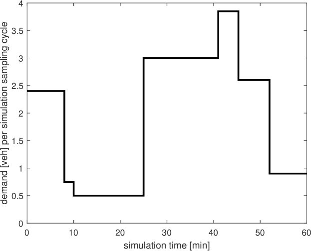
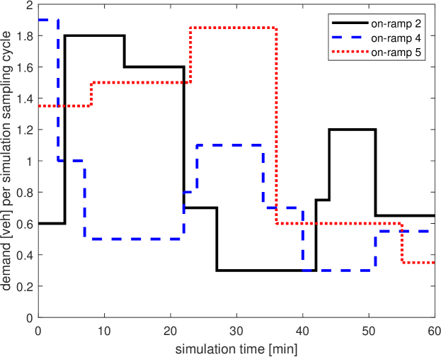
Figure 11: Demand profiles of the mainstream road (top plot) and of the on-ramps (bottom plot) used for the case study.

IV-B Base and parallel controllers

\psfrag{ev}[0.8]{Evaluate}\psfrag{10}[0.8]{\eqref{eq:Alinea}}\psfrag{ANN}[0.8]{ANN}\psfrag{Alinea}[0.8]{ALINEA}\psfrag{high}[0.8]{Highway (ACTM with disturbed external inputs)}\psfrag{ACTM}[0.8]{ACTM}\psfrag{pmpc1}[0.8]{PMPC(1)}\psfrag{pmpc2}[0.8]{PMPC(2)}\psfrag{cmpc1}[0.8]{CMPC(1)}\psfrag{cmpc2}[0.8]{CMPC(2)}\psfrag{base}[0.8]{Base block}\psfrag{par}[0.8]{Parallel block}\psfrag{theta}[0.8]{$\bm{\theta}^{\textrm{ALINEA}}(k)$}\psfrag{mu}[0.8]{$\bm{\mu}(k)$}\psfrag{state }[0.8]{states and external inputs}\psfrag{mutildei}[0.8]{$\tilde{\bm{\theta}}^{\textrm{BCi}}(k;n^{\textrm{H}}(1)),\tilde{\bm{\theta}}^{\textrm{BCi}}(k;n^{\textrm{H}}(2))$}\psfrag{mutildee}[0.8]{$\tilde{\bm{\mu}}^{\textrm{BCe}}(k;n^{\textrm{H}}(1)),\tilde{\bm{\mu}}^{\textrm{BCe}}(k;n^{\textrm{H}}(2))$}\psfrag{mup1}[0.8]{$\tilde{\bm{\mu}}^{\textrm{PMPC(1)}}(k;\bar{n}^{\textrm{e}})$}\psfrag{mup2}[0.8]{$\tilde{\bm{\mu}}^{\textrm{PMPC(2)}}(k;\bar{n}^{\textrm{e}})$}\psfrag{muc2}[0.8]{$\tilde{\bm{\mu}}^{\textrm{CMPC(2)}}(k;\bar{n}^{\textrm{e}})$}\psfrag{muc1}[0.8]{$\tilde{\bm{\mu}}^{\textrm{CMPC(1)}}(k;\bar{n}^{\textrm{e}})$}\psfrag{muANN}[0.8]{$\tilde{\bm{\mu}}^{\textrm{ANN}}(k;\bar{n}^{\textrm{e}})$}\psfrag{muA}[0.8]{$\tilde{\bm{\mu}}^{\textrm{ALINEA}}(k;\bar{n}^{\textrm{e}})$}\psfrag{select}[0.8]{Selector}\psfrag{tttp1}[0.7]{$J^{\textrm{PMPC(1)}}(k)$}\psfrag{tttp2}[0.7]{$J^{\textrm{PMPC(2)}}(k)$}\psfrag{tttc2}[0.7]{$J^{\textrm{CMPC(2)}}(k)$}\psfrag{tttc1}[0.7]{$J^{\textrm{CMPC(1)}}(k)$}\psfrag{tttANN}[0.7]{$J^{\textrm{ANN}}(k)$}\psfrag{tttA}[0.7]{$J^{\textrm{ALINEA}}(k)$}\psfrag{mubest}[0.8]{$\bm{\mu}^{\textrm{best}}(k)$}\includegraphics[width=433.62pt]{controller_case_study}

Figure 12: The base-parallel integrated control architecture implemented to the stretch of the highway for the case study.

The base-parallel control architecture we have used for this case study is illustrated in Figure 12. In the base block, we have considered an explicit (ALINEA) and an implicit (ANN) base controller, which are detailed next. ALINEA [22] is a feedback-based control approach for ramp metering in road traffic. The control signal produced by ALINEA for the control sampling time step $k$ for the ramp meter of on-ramp $i$ is

$$\mu_{i}(k)=\max\Big{\{}\mu_{i}(k-1)+\theta^{\textrm{ALINEA}}_{i}(k)\left(\rho^{\textrm{crit}}_{i}-\rho_{i}(k)\right),0\Big{\}},$$ (14)

with $\theta^{\textrm{ALINEA}}_{i}(k)$ the tuning parameter of ALINEA for cell $i$ at the control sampling time step $k$, and $\rho^{\textrm{crit}}_{i}$ and $\rho_{i}(k)$ the critical and measured densities (i.e., total number of vehicles per unit length per lane) of cell $i$ at the control sampling time step $k$ directly downstream of on-ramp $i$. For the ALINEA block, we apply the constant gain of $\theta^{\textrm{ALINEA}}=0.016$ from [23], when using the SI units for the variables in (14). Moreover, the values (given in [veh] per simulation sampling cycle) $\mu_{2}=0.5,\ \mu_{4}=0.2,$ and $\mu_{5}=0.4$ are used as the previous control signals in order to evaluate the control signal of ALINEA for the initial simulation sampling time step. For $\rho^{\textrm{crit}}_{i}$, we use $0.0335$ veh/m/lane [24] for all the 6 cells shown in Figure 10. Note that since $\rho_{i}(k)$ is not computed directly as a state variable via the ACTM, we should compute it at every control sampling time step in veh/m/lane, which based on the definition of the density, is determined by $\rho_{i}(k)=n_{i}(k)/(\textrm{cell length})$, reminding that the highway of the case study is single-lane. In Figure 12, the vector $\bm{\mu}(k)$ includes $\mu_{2}(k)$, $\mu_{4}(k)$, and $\mu_{5}(k)$, i.e., the ALINEA block illustrated in Figure 12 includes the control policy of (14) and hence, the tuned parameters of ALINEA for all the three metered on-ramps.

\psfrag{ANN}[.8]{ANN for cell $i$}\psfrag{q}[.8]{$q_{i}(k)$}\psfrag{n}[.8]{$n_{i}(k)$}\psfrag{theta}[.8]{$\theta^{\textrm{ALINEA}}_{i}(k)$}\psfrag{d}[.8]{$d_{i}(k)$}\psfrag{o}[.8]{$o_{i-1}(k)$}\includegraphics[width=238.49231pt]{ANN}

\psfrag{ANN}[.8]{ANN for cell $i$}\psfrag{q}[.8]{$q_{i}(k)$}\psfrag{n}[.8]{$n_{i}(k)$}\psfrag{theta}[.8]{$\theta^{\textrm{ALINEA}}_{i}(k)$}\psfrag{d}[.8]{$d_{i}(k)$}\psfrag{o}[.8]{$o_{i-1}(k)$}\includegraphics[width=433.62pt]{test}

Figure 13: The ANN-based mapping used as an implicit base controller per cell for the case study.

For the implicit base controller, a mapping based on an artificial neural network (ANN) is trained (see Figure 13), which receives the state variables $n_{i}(k)$ and $q_{i}(k)$ and the uncontrolled external inputs $d_{i}(k)$ and $o_{i-1}(k)$ of a cell for every control sampling time step $k$, and produces a value for $\theta^{\textrm{ALINEA}}_{i}(k)$ in (14). The ANN is a feedforward network with one hidden layer of size three. To train this mapping, we have generated a dataset of size $500$, including $n_{i}$, $q_{i}$, $d_{i}$, and $o_{i-1}$ with $i=2,4,5$ for $500$ various traffic scenarios as the inputs of the ANN for cell $i$, and optimized values of $\theta^{\textrm{ALINEA}}_{i}(k)$ as the output. The input values are considered such that a wide range of possible scenarios is covered. To generate the output values, we consider each metered cell as an isolated one, i.e., with infinite capacity for the leaving flows, and minimize the difference between the critical density $\rho^{\textrm{crit}}_{i}$ and the cell’s expected density $\rho^{\textrm{exp}}_{i}(k+1)$ with respect to $\theta^{\textrm{ALINEA}}_{i}(k)$ as the optimization variable. This is because the objective of ALINEA is to keep the road’s density downstream of an on-ramp near the critical density (see (14) and [25]). The expected density is determined by dividing the expected total number of vehicles $n^{\textrm{exp}}_{i}(k+1)$ in cell $i$ by the length of the cell, with

$$n^{\textrm{exp}}_{i}(k+1)=n_{i}(k)+o_{i-1}(k)+e_{i}(k)-o_{i}(k)-s_{i}(k),$$

where $e_{i}(k)$ is computed by the second formulation of (12) and $\mu_{i}(k)$ by (14). The generated dataset is divided into a training dataset including 400 data, and a validation dataset including the rest 100 data. Note that the ANN in Figure 12 includes three mappings for the three ramp meters, i.e., the vector $\bm{\theta}^{\textrm{ALINEA}}(k)$ includes $\theta^{\textrm{ALINEA}}_{2}(k)$, $\theta^{\textrm{ALINEA}}_{4}(k)$, and $\theta^{\textrm{ALINEA}}_{5}(k)$. For the case study, in addition to the initial state of the network and the initial values of the measured demands, we have used $o_{1}(0)=3.8,\ o_{3}(0)=3.2,$ and $o_{4}(0)=0.6$ (given in [veh] per simulation sampling cycle) to evaluate the outputs of the three ANN-based mappings for the initial simulation sampling time step. The output $\bm{\theta}^{\textrm{ALINEA}}(k)$ of the ANN is first transformed into $\bm{\mu}(k)$ using (14) (see Figure 12). The ACTM is then used to generate a sequence $\tilde{\bm{\mu}}$ using the control inputs generated by the ALINEA and the ANN blocks.

For each base controller, we consider a parallel cell with two MPC-based controllers, where for the explicit base controller (ALINEA), the MPC-based controllers (CMPC(1) and CMPC(2) in Figure 12) are formulated using conventional MPC, and for the implicit base controller (ANN), parameterized MPC (PMPC(1) and PMCP(2) in Figure 12) is used. We use the “fmincon” solver with multiple starting optimization points and the Sequential Quadratic Programming (SQP) algorithm from the Matlab optimization toolbox, to solve the MPC optimization problems, which, in general, are nonlinear and non-convex. The function tolerance and the step tolerance are set to, respectively, $10^{-3}$ and $10^{-7}$. The cost function $J(k)$ of the MPC optimization problems at the control sampling time step $k$ is defined by

$$J(k)=\textrm{TT}(k)-\gamma\textrm{TD}(k),$$ (15)

with TT and TD the travel time and the traveled distance of all the vehicles. We have used $\gamma=0.8$ for the simulations. The MPC optimization problems are subject to constraints, including the traffic dynamics, upper and lower bounds for the ramp meters, and lower bound for the queue lengths on the on-ramps.

The main difference between the two MPC-based controllers indexed by 1 and 2 in each cell is in the size of their prediction horizons $n^{\textrm{H}}(1)$ and $n^{\textrm{H}}(2)$, i.e., 3 and 10. More specifically, CMPC(1) and PMPC(1) have the prediction horizon $n^{\textrm{H}}(1)$ and CMPC(2) and PMPC(2) have the prediction horizon $n^{\textrm{H}}(2)$. Note that a large prediction horizon provides a more extensive vision of the future, which may help to reduce the negative effects of the finite horizon of MPC on the degree of optimality of the solutions. However, the cumulative errors resulting from the inaccuracies in the prediction model are larger for a larger prediction horizon.

The candidate control inputs produced by ANN, ALINEA, PMPC(1), PMPC(2), CMPC(1), and CMPC(2) are all sent to the evaluation block (see Figure 12), where six ACTM blocks will in parallel estimate the realized value of the cost function of all the vehicles for a prediction time horizon of size $\bar{n}^{\textrm{e}}$ (assuming that $\bar{n}^{\textrm{e}}\leq n^{\textrm{H}}(1)<n^{\textrm{H}}(2)$) for each candidate control input. We have used $\bar{n}^{\textrm{e}}=3$ for the case study. The “Selector” compares these values and selects the control input $\bm{\mu}^{\textrm{best}}(k)$ that corresponds to the minimum cost.

IV-C Results

Table II: The results of a 1-hour simulation for the case study.

control approach	$J^{\textrm{total}}={\displaystyle\sum_{k}}\ \left(\textrm{TT}(k)-\gamma\textrm{TD}(k)\right)$ [h]	$n^{\textrm{total}}$ [veh]	average cost per vehicle [s]
Alinea	455.95	6.1342 $\times 10^{4}$	26.76
ANN	431.71	6.4531 $\times 10^{4}$	24.08
CMPC(1)	412.76	6.7738 $\times 10^{4}$	21.94
CMPC(2)	412.76	6.7738 $\times 10^{4}$	21.94
PMPC(1)	412.91	6.7710 $\times 10^{4}$	21.95
PMPC(2)	412.91	6.7679 $\times 10^{4}$	21.96
Base-parallel architecture	412.69	6.7582 $\times 10^{4}$	21.98

Table II includes the results of the case study for a 1-hour simulation repeated with different control approaches, Alinea, ANN, CMPC(1), CMPC(2), PMPC(1), PMPC(2), and the base-parallel control architecture given by Figure 12. Since, in general, the optimization problems of the MPC-based controllers are non-convex, the optimization solvers may return a locally optimal solution instead of a global optimum. In order to deal with this problem, we have proposed three different starting points for the MPC optimization solvers, i.e.,

• solution of the optimization corresponding to the previous control sampling time step, ignoring the first element of the sequence and repeating the last element twice;

• average of the solution of the optimization corresponding to the previous control sampling time step (ignoring the first element of the sequence and repeating the last element twice) and the solution of the optimization corresponding to the second previous control sampling time step (ignoring the first two elements of the sequence and repeating the last element three times), where this starting point can be used for $k\geq 2$;

• average of the solution of the optimization corresponding to all the previous control sampling time steps (ignoring those elements of the sequences that correspond to the past control sampling time steps and repeating the last elements to cover the prediction time window).

In Table II for each control approach, we have represented the realized value of the total cost function, $J^{\textrm{total}}$, in [h] for the 1-hour simulation period, which has been computed via (15) per control sampling time step and accumulated across the simulation time window. The total number of vehicles, $n^{\textrm{total}}$, that can travel through the controlled stretch of the road within the fixed simulation time window is another indication for the control performance. In other words, we expect a high-performing control approach to minimize $J^{\textrm{total}}$, while allowing higher numbers of vehicles that intend to enter the stretch of the road to travel via it in the given simulation time window. Therefore, the ratio of these two values, i.e., the average cost per vehicle, can be an indication of the control performance. The lower this ratio, the better the control approach. Hence, in Table II we have also represented $n^{\textrm{total}}$ in [veh] and the average cost per vehicle in [s] (i.e., $J^{\textrm{total}}*3600$ divided by $n^{\textrm{total}}$), for all the control approaches used in the case study.

Based on the results given in Table II, CMPC(1), CMPC(2), PMPC(1), and PMPC(2) result in the lowest values for the average cost per vehicle. Comparing the three real-time control approaches (i.e., they can always produce their candidate control inputs in a time budget smaller than or equal to the control sampling time of the controlled system) ALINEA, ANN, and the proposed base-parallel control architecture, the lowest average cost per vehicle corresponds to the proposed base-parallel control architecture. It is also important to indicate that among all the 7 control approaches considered in this case study, the proposed base-parallel control approach results in the lowest value of the total cost.

V Discussion

The conventional and parameterized MPC approaches have resulted in the best performance among the other control methods used in the case study. This is somehow expected since MPC approaches minimize the cost function at every control sampling time step by solving an online optimization problem, based on the updated measured values of the state and uncontrolled external inputs. The main issue with MPC, however, is the high computation time, which may exceed the control sampling cycle of the controlled system, especially when the scales of the controlled system and the complexity of the dynamics increase. Moreover, due to the non-convexity of the optimization problem, several starting optimization points should be considered to make sure more sub-regions in the optimization search region are covered. This will cause increased computational burden and computation time.

However, when the MPC-based approaches are used in the proposed parallel block, the issue with the computational burden and computation time can be tackled due to the following reasons:

• The MPC-based controllers are given a time budget that is smaller than or equal to the control sampling time of the controlled system. Therefore, the control system will not wait longer than this time budget, and in case the control inputs returned by any of the MPC-based controllers result in a non-satisfactory performance, they will be excluded by the evaluation block and the selector.

• Several MPC-based controllers will run in parallel, i.e., instead of running one MPC module in a serial set-up with various optimization starting points (as for CMPC(1), CMPC(2), PMPC(1), and PMPC(2)), they will be run in parallel. Therefore, the computational burden is distributed among the parallel MPC-based controllers, which results in reduced computation time.

• The existence of the base block next to the online MPC-based controllers provides a warm-start for them that reduces the computational burden and the computation time, which are large for the conventional and parameterized MPC-based controllers, CMPC(1), CMPC(2), PMPC(1), and PMPC(2), due to an extensive exploration of the optimization search region.

Moreover, a detailed assessment of the prediction horizon for real-life processes is not possible prior to running the control procedure, particularly when the nonlinearities increase. Therefore, we allow both a small and a large prediction horizon for the MPC-based controllers via the use of parallel cells within the proposed control architecture.

The lower value of the realized total cost function corresponding to the base-parallel control architecture in comparison with the MPC-based approaches that aim at minimizing the same cost function online at every control sampling time step, together with the fact that for the majority of the control sampling time steps, one of the MPC-based controllers has won the competition in the evaluation block, may be explained via the following reason. The warm-start provided via the base block for the online MPC optimization problems in the parallel block, has improved the performance of these controllers for several control sampling time steps. In other words, although we may provide several starting points for the online MPC optimization problems, this will not guarantee that the entire optimization search region will necessarily be covered. More specifically, this will not guarantee that the sub-regions that correspond to global or better local optima will be covered, while the warm-start provided by the base block has in several cases allowed the online optimizers to search such sub-regions.

VI Conclusions and Future Work

We have proposed an integrated base-parallel control architecture with the aim of addressing the current gap in efficient real-time implementation of MPC-based control approaches for highly nonlinear systems with fast dynamics and a large number of control constraints. In this architecture, several offline tuned or optimized controllers and online optimization-based controllers can run in parallel.

We have performed a simulation for controlling the metered on-ramps of a stretch of a highway. The simulation results have shown that, among the control approaches that can perform in real time, the proposed base-parallel control architecture has the performance (considering the average cost per vehicle) that is the closest to the online MPC-based controllers, which produce optimal control inputs, but suffer from high computation times. Moreover, the least value of the overall cost among all these 7 control approaches, corresponds to the base-parallel control architecture. The new control architecture results in a control system that is very flexible and its architecture can easily be changed or modified online.

Relevant topics that require further exploration in the future include:

• Stability analysis of the proposed base-parallel control architecture, assuming individually stable base and parallel controllers.

• More extensive simulations including various large-scale controlled systems with highly nonlinear dynamics, and including different base and parallel controllers.

• In-depth study and analysis of the influences of different tuning parameters of MPC for various dynamics of the controlled system. This can be done by running several parallel MPC-based controllers in the parallel block and tracking the trend of the selection of each candidate control input based on the ongoing dynamics of the controlled system.

Anahita Jamshidnejad received the PhD degree in Systems and Control from the Delft University of Technology, the Netherlands. She is currently an Assistant Professor at the Faculty of Aerospace Engineering, Delft University of Technology. Her research interests include optimization theory in engineering problems, integrated control methods, and model-predictive control, with applications in robotic systems and road traffic.

Gabriel Gomes received the PhD degree in systems and control theory from the Department of Mechanical Engineering, University of California at Berkeley. He is currently an Assistant Research Engineer with the Institute for Transportation Studies, University of California at Berkeley. His research focuses on the modeling, control, and simulation of transportation systems.

Alexandre M. Bayen is the Liao-Cho Professor of Engineering at UC Berkeley. He received the PhD degree in Aeronautics and Astronautics from Stanford University. He was a visiting researcher with the NASA Ames Research Center, from 2000 to 2003. Since 2014, he has been the Director of the Institute for Transportation Studies. He is also a Faculty Scientist in Mechanical Engineering, at the Lawrence Berkeley National Laboratory.

Bart De Schutter (IEEE member since 2008, senior member since 2010, and IEEE Fellow since 2019) is a full professor and head of department at the Delft Center for Systems and Control of Delft University of Technology in Delft, The Netherlands. He is Senior Editor of the IEEE Transactions on Intelligent Transportation Systems. His current research interests include intelligent transportation and infrastructure systems, hybrid systems, and multi-level and multi-agent control of large-scale systems.

References

- [1] J. Maciejowski, Predictive Control with Constraints. London, UK: Prentice Hall, 2002.
- [2] B. Huyck, H. J. Ferreau, M. Diehl, J. De Brabanter, J. F. M. Van Impe, B. De Moor, and F. Logist, “Towards online model predictive control on a programmable logic controller: Practical considerations,” Mathematical Problems in Engineering, vol. 2012, pp. 1–20, 2012.
- [3] B. Huyck, J. De Brabanter, J. F. Van Impe, and F. Logist, “Online model predictive control of industrial processes using low level control hardware: A pilot-scale distillation column case study,” Control Engineering Practice, vol. 28, pp. 34–48, 2014.
- [4] Y. Wang and S. Boyd, “Fast model predictive control using online optimization,” IEEE Transactions on Control Systems Technology, vol. 18, no. 2, pp. 267–278, 2010.
- [5] B. Houska, H. J. Ferreau, and M. Diehl, “An auto-generated real-time iteration algorithm for nonlinear MPC in the microsecond range,” Automatica, vol. 47, no. 10, pp. 2279–2285, 2011.
- [6] A. Bemporad, M. Morari, V. Dua, and E. N. Pistikopoulos, “The explicit linear quadratic regulator for constrained systems,” Automatica, vol. 38, no. 1, pp. 3–20, 2002.
- [7] T. A. Johansen, “On multi-parametric nonlinear programming and explicit nonlinear model predictive control,” in 41st IEEE Conference on Decision and Control, Las Vegas, USA, December 2002, pp. 2768–2773.
- [8] A. Bemporad and C. Filippi, “An algorithm for approximate multiparametric convex programming,” Computational Optimization and Applications, vol. 35, no. 1, pp. 87–108, 2006.
- [9] A. Alessio and A. Bemporad, Nonlinear Model Predictive Control Lecture Notes in Control and Information Sciences. Berlin, Germany: Springer, 2009, vol. 384, ch. A Survey on Explicit Model Predictive Control.
- [10] M. N. Zeilinger, C. N. Jones, and M. Morari, “Real-time suboptimal model predictive control using a combination of explicit MPC and online optimization,” IEEE Transactions on Automatic Control, vol. 56, no. 7, pp. 1524–1534, 2011.
- [11] S. K. Zegeye, B. De Schutter, J. Hellendoorn, E. A. Breunesse, and A. Hegyi, “A predictive traffic controller for sustainable mobility using parameterized control policies,” IEEE Transactions on Intelligent Transportation Systems, vol. 13, no. 3, pp. 1420–1429, 2012.
- [12] M. Muehlebach and R. D’Andrea, “Parameterized infinite-horizon model predictive control for linear time-invariant systems with input and state constraints,” in American Control Conference (ACC), Boston, USA, July 2016, pp. 2669–2674.
- [13] R. Cagienard, P. Grieder, E. C. Kerrigan, and M. Morari, “Move blocking strategies in receding horizon control,” Journal of Process Control, vol. 17, no. 6, pp. 563–570, 2007.
- [14] R. C. Shekhar and C. Manzie, “Optimal move blocking strategies for model predictive control,” Automatica, vol. 61, pp. 27–34, 2015.
- [15] L. Grüne and J. Pannek, Nonlinear Model Predictive Control: Theory and Algorithms. London, UK: Springer-Verlag, 2011.
- [16] A. Bemporad and C. Filippi, “Suboptimal explicit receding horizon control via approximate multiparametric quadratic programming,” Journal of Optimization Theory and Applications, vol. 117, no. 1, pp. 9–38, 2003.
- [17] W. H. Chen, D. J. Ballance, and J. O’Reilly, “Model predictive control of nonlinear systems: Computational burden and stability,” IEE Proceedings - Control Theory and Applications, vol. 147, no. 4, pp. 387–394, 2000.
- [18] M. Alamir, “Fast NMPC: A reality-steered paradigm: Key properties of fast NMPC algorithms,” in European Control Conference, Strasbourg, France, June 2014, pp. 2472–2477.
- [19] S. Gros, M. Zanon, R. Quirynen, A. Bemporad, and M. Diehl, “From linear to nonlinear MPC: Bridging the gap via the real-time iteration,” International Journal of Control, pp. 1–19, 2016.
- [20] G. Gomes and R. Horowitz, “Optimal freeway ramp metering using the asymmetric cell transmission model,” Transportation Research Part C: Emerging Technologies, vol. 14, no. 4, pp. 244–262, 2006.
- [21] L. Muñoz, X. Sun, D. Sun, G. Gomes, and R. Horowitz, “Methodological calibration of the cell transmission model,” in American Control Conference, Boston, USA, July 2004, pp. 798–803.
- [22] M. Papageorgiou, H. Hadj-Salem, and J. Blosseville, “ALINEA: A local feedback-based control law for on-ramp metering,” Transportation Research Rescord, vol. 1, no. 1320, pp. 58–67, 1991.
- [23] M. Papageorgiou, “Modeling and real-time control of traffic flow on the southern part of boulevard Peripherique in Paris: Part II: Coordinated on-ramp metering,” Transportation Research Part A, vol. 24A, no. 5, pp. 361–370, 1990.
- [24] A. Hegyi, B. De Schutter, and H. Hellendoorn, “Model predictive control for optimal coordination of ramp metering and variable speed limits,” Transportation Research Part C, vol. 13, no. 3, pp. 185–209, Jun. 2005.
- [25] G. van de Weg, A. Hegyi, S. Hoogendoorn, and B. De Schutter, “Efficient freeway MPC by parameterization of ALINEA and a speed-limited area,” IEEE Transactions on Intelligent Transportation Systems, vol. 20, no. 1, pp. 16–29, 2019.