TUM-HEP-1210/19
July 11, 2019

Violation of the Kluberg-Stern-Zuber theorem
in SCET

Martin Beneke,^a Mathias Garny,^a Robert Szafron,^a Jian Wang^a,b

^aPhysik Department T31,
James-Franck-Straße 1, Technische Universität München,
D–85748 Garching, Germany
^bSchool of Physics, Shandong University, Jinan, Shandong 250100, China

A classic result, originally due to Kluberg-Stern and Zuber, states that operators that vanish by the classical equation of motion (eom) do not mix into “physical” operators. Here we show that and explain why this result does not hold in soft-collinear effective theory (SCET) for the renormalization of power-suppressed operators. We calculate the non-vanishing mixing of eom operators for the simplest case of $N$-jet operators with a single collinear field in every direction. The result implies that—for the computation of the anomalous dimension but not for on-shell matrix elements—there exists a preferred set of fields that must be used to reproduce the infrared singularities of QCD scattering amplitudes. We identify these fields and explain their relation to the gauge-invariant SCET Lagrangian. Further checks reveal another generic property of SCET beyond leading power, which will be relevant to resummation at the next-to-leading logarithmic level, the divergence of convolution integrals with the hard matching coefficients. We propose an operator solution that allows to consistently renormalize such divergences.

1 Introduction

Operators that vanish by the classical equation of motion (eom) are usually considered redundant in the construction of an operator basis for an effective field theory (EFT) because the EFT is only designed to reproduce the on-shell scattering amplitudes of the low-energy degrees of freedom. Indeed, eom operators do not affect on-shell S-matrix elements (see e.g. [1, 2]), including infrared (IR) divergent matrix elements, provided the IR divergences are logarithmic [1]. This is closely related to the fact that quantum fields provide a highly redundant representation of the S-matrix, which remains invariant under a large class of field redefinitions in writing the action of the theory.

Moreover, a well-known result due to Kluberg-Stern and Zuber [3] states that eom operators (also termed “class II”) do not mix into physical (“class I”) operators under renormalization (see also [4, 1] and [5, 6, 7, 8] for other aspects of the statement), which implies a triangular structure of the operator anomalous dimension matrix (ADM). This does not mean that eom operators can always be ignored in ADM computations. For example, if an off-shellness is employed to regulate IR divergences, or if, in the case of gauge theories, an IR regulator is used that breaks gauge invariance, counterterms proportional to eom operators may be necessary to remove subdivergences (see, for instance, [9]). However, in the final ADM, the eom operators still mix only among themselves and do not influence the evolution of the couplings of the physical operators. Given the relation to field redefinitions, the triangular structure of the ADM is required by the consistency of the EFT since otherwise the ADM of the physical operators would depend on the arbitrary field representation employed to compute the S-matrix.

The scattering amplitudes of massless particles in gauge theories exhibit IR singularities due to the emission and loops of soft and collinear particles. In dimensional regularization (space-time dimension $d=4-2\epsilon$), contrary to ultraviolet (UV) divergences, a double $1/\epsilon^{2}$ pole appears at the one-loop order, and up to $1/\epsilon^{2n}$ at the $n$th loop order. Referring to QCD in the following, the EFT that describes the high-energy scattering of massless partons (quarks and gluons) is soft-collinear effective theory (SCET) [10, 11, 12, 13]. The IR divergences of the QCD S-matrix appear as UV divergences of certain collinear field operators in SCET [14]. Hence, the study of IR divergences and resummation of large IR logarithms in QCD can be phrased as an operator-mixing and renormalization-group problem in SCET.

This is well understood at leading power (LP) in the EFT expansion and has found many applications in collider physics. In this context, the expansion parameter of the EFT is defined as follows. Let $Q$ be the scale of a hard process that involves a number of jets. The typical transverse momentum $p_{\perp}\sim Q\lambda$ of partons within a jet defines the power counting parameter $\lambda\ll 1$ of SCET. The collinear modes within a jet can interact with other jets through the exchange of soft modes with momentum $k\sim Q\lambda^{2}$, which preserve the virtuality of collinear modes within jets. While the SCET Lagrangian beyond the leading power has been known for a long time [12, 13] and the first systematic study of power-suppressed effects and their factorization has been undertaken in the early days of SCET for the production of a single jet of hadrons in semi-leptonic $B$-meson decay [15], a more complete investigation of SCET beyond LP has started only recently [16, 17, 18, 19, 20, 21, 22, 23, 24, 25, 26]. In particular, the ADM of $N$-jet operators at next-to-leading power (NLP) $\mathcal{O}(\lambda,\lambda^{2})$ has been computed at the one-loop order [22, 23].

In this work, we show that the ADM of $N$-jet operators at sub-leading power in SCET violates the Kluber-Stern-Zuber (KSZ) theorem. In other words, we demonstrate that eom operators mix into physical operators. The mixing is in fact required to reproduce the IR divergences of QCD amplitudes from SCET. We explain where the proof of KSZ fails, why—contrary to the statements in the first two paragraphs of this introduction—SCET is nevertheless a sensible EFT of QCD. We discuss several checks. They reveal another generic property of SCET beyond LP, which, although it has appeared in some applications [30, 31], has not yet been fully recognized: the divergence of the convolution integrals of hard coefficient functions with the SCET matrix element. We provide a rearrangement of the operator basis of $\mathcal{O}(\lambda)$ operators that can be consistently renormalized in the presence of singular convolutions with hard-matching coefficients. In the subsequent presentation we explain these issues, which are of interest from a general quantum-field theoretic point of view, in the simplest case. A complete treatment of SCET operator mixing at NLP including $\mathcal{O}(\lambda^{2})$ mixing, as is relevant to NLP resummation at next-to-leading logarithmic accuracy, based on the techniques developed here is quite involved. We leave this to a longer and more technical paper [32].

2 Lorentz invariance implies soft mixing

That something peculiar is going on with operator mixing in SCET beyond LP can be inferred from the following simple consideration. A LP $N$-jet operator is a product of $N$ collinear fields from $\{W_{k}^{\dagger}\xi_{k},\,\bar{\xi}_{k}W_{k},W_{k}^{\dagger}[iD_{\perp k}^{\mu}W_{k}]\}\equiv\{\chi_{k},\bar{\chi}_{k},{\cal A}_{\perp k}^{\mu}\}$, representing the collinear-gauge-invariant collinear quark, antiquark and gluon fields, respectively, where $k=1,\ldots N$ specifies the well-separated directions of the $N$ jets. The ADM of these operators up to the two-loop order has the form

$$\mathbf{\Gamma}=-\gamma_{\rm cusp}(\alpha_{s})\sum_{k<j}\mathbf{T}_{k}\cdot\mathbf{T}_{j}\ln\left(\frac{-s_{kj}}{\mu^{2}}\right)+\sum_{k}\gamma_{k}(\alpha_{s})$$ (1)

in colour-operator notation [33] and for all out-going momenta $p_{k}$ at the operator vertex, $s_{kj}=2p_{k}\cdot p_{j}+i0$, $k,j=1\ldots N$. Here $\gamma_{\rm cusp}$ is the universal cusp anomalous dimension, while $\gamma_{k}$ are the contributions to the anomalous dimension associated to each collinear direction $k$. For an $N$-particle scattering amplitude with exactly one line in every direction, it is natural to align the light-like vectors $n_{k-}$ with the momentum $p_{k}$ such that $p_{k}^{\mu}=(n_{k+}p_{k})\,n_{k-}^{\mu}/2$. In this case the above anomalous dimension is exact to all orders in the power expansion, in the sense that it generates the IR divergences of the full QCD amplitude, since operators with transverse derivatives have vanishing matrix elements.

However, it is equally possible to slightly misalign the reference vectors $n_{k-}$ defining the collinear directions $k$, provided that the components of $p_{k}$ scale as $(n_{k+}p,p_{\perp k},n_{k-}p)\sim(1,\lambda,\lambda^{2})$. Lorentz invariance implies that the anomalous dimension remains as in (1), but the power expansion of SCET requires that it should be expanded for this situation. Defining

$$s^{(0)}_{kj} = \frac{1}{2}(n_{k-}n_{j-})(n_{k+}p_{k})(n_{j+}p_{j})\,,$$ (2)

$$s_{kj} = s^{(0)}_{kj}+(n_{k+}p_{k})(n_{k-}p_{\perp j})+(n_{j+}p_{j})(n_{j-}p_{\perp k})+\mathcal{O}(\lambda^{2})\,,$$ (3)

we find

$$\mathbf{\Gamma} = -\gamma_{\rm cusp}(\alpha_{s})\sum_{k<j}\mathbf{T}_{k}\cdot\mathbf{T}_{j}\ln\left(\frac{-s_{kj}^{(0)}}{\mu^{2}}\right)+\sum_{k}\gamma_{k}(\alpha_{s})$$ (4)

$$-\,\gamma_{\rm cusp}(\alpha_{s})\sum_{k\not=j}\mathbf{T}_{k}\cdot\mathbf{T}_{j}\frac{2n_{j-}p_{\perp k}}{(n_{k-}n_{j-})(n_{k+}p_{k})}+\mathcal{O}(\lambda^{2})\,.$$

The $\mathcal{O}(\lambda)$ term in the second line implies non-vanishing operator mixing of the LP $N$-jet operator into NLP $N$-jet operators with an additional derivative $i\partial^{\mu}_{\perp k}$ acting on one of the collinear building blocks. The corresponding one-loop anomalous dimension in notation as in (2.17) of [23] is given by

$$\gamma^{kj}_{P_{i}Q_{i}}=\frac{\alpha_{s}}{\pi}\,{\bf T}_{k}\cdot{\bf T}_{j}\,\frac{n_{j-}^{\mu}\delta_{ki}}{(n_{k-}n_{j-})(n_{i+}p_{i})}+(k\leftrightarrow j)\,,$$ (5)

where $P_{i}=J^{A0}_{1}\ldots J^{T1}_{i}\ldots J^{A0}_{N}$ is an $N$-jet operator with LP building blocks $J^{A0}_{j}\in\{\chi_{j},\bar{\chi}_{j},{\cal A}_{\perp j}^{\mu}\}$ for $j\not=i$, and a time-ordered product with a sub-leading power soft-collinear Lagrangian interaction $\mathcal{L}_{i}^{(1)}(x)$ at order $\lambda$,

$$J^{T1}_{i}(t_{i})\equiv i\int d^{4}x\,T\big{\{}J_{i}^{A0}(t_{i}),\mathcal{L}_{i}^{(1)}(x)\big{\}}\,,$$ (6)

for $j=i$. Furthermore, $Q_{i}=J^{A0}_{1}\ldots J^{A1\,\mu}_{i}\ldots J^{A0}_{N}$ is an $\mathcal{O}(\lambda)$ suppressed current operator with $J^{A1\,\mu}_{i}(t_{i})\equiv i\partial_{\perp i}^{\mu}J^{A0}_{i}(t_{i}n_{i+})$. In the notation of [22, 23], this corresponds to the operator mixing

$$J^{T1}_{i}(t_{i})\to J^{A1\,\mu}_{i}(t_{i})\,,$$ (7)

through a soft loop. However, it was shown by explicit computation [22, 23] that no such soft mixing exists, in contradiction with the above conclusion.

The correctness of (5) follows from another argument. Lorentz invariance is broken in SCET by the reference vectors $n_{k-}$, but the implications of Lorentz invariance are instead encoded in reparameterization invariance (RPI) under changes of the arbitrary reference vectors [34]. Without loss of generality (due to the dipole structure of the anomalous dimension at one loop), we consider $N=2$ and focus on the power-suppressed operators in the $i$-direction and $i<j$. RPI invariance implies that $J^{(A0,A0)}$ and $J^{(A1,A0)}$ must appear in the combination

$$\int dsdt\,C^{(A0,A0)}(t,s)\,\bar{\chi}_{j}(sn_{j+})\Gamma\left[1+\frac{2t}{n_{i-}n_{j-}}\,n_{j-}\cdot\partial_{\perp i}\right]\chi_{i}(tn_{i+})\,,$$ (8)

where $\Gamma$ is some Dirac matrix. In momentum space, the factor of $t$ is transformed into the derivative $(-i)\partial/\partial n_{i+}p_{i}$ acting on the momentum-space coefficient $C^{(A0,A0)}(n_{i+}p_{i},n_{j+}p_{j})$, and the hard matching coefficients of $J^{(A0,A0)}$ and $J^{(A1,A0)}$ are therefore related as

$$C^{(A1,A0)\,\mu}(n_{i+}p_{i},n_{j+}p_{j})=\frac{-2n_{j-}^{\mu}}{n_{i-}n_{j-}}\frac{\partial}{\partial n_{i+}p_{i}}\,C^{(A0,A0)}(n_{i+}p_{i},n_{j+}p_{j})\,.$$ (9)

This equation implies the renormalization group equation

$$\frac{d}{d\ln\mu}\,C^{(A1,A0)\,\mu}(n_{i+}p_{i},n_{j+}p_{j}) = -\bigg{[}\gamma_{\rm cusp}(\alpha_{s}){\bf T}_{i}\cdot{\bf T}_{j}\ln\frac{-s_{ij}^{(0)}}{\mu^{2}}+\gamma_{i}\bigg{]}C^{(A1,A0)\,\mu}(n_{i+}p_{i},n_{j+}p_{j})$$ (10)

$$+\,\gamma_{\rm cusp}(\alpha_{s}){\bf T}_{i}\cdot{\bf T}_{j}\frac{2n_{j-}^{\mu}}{(n_{i-}n_{j-})n_{i+}p_{i}}\,C^{(A0,A0)}(n_{i+}p_{i},n_{j+}p_{j})$$

for the coefficient function of the power-suppressed operator, as can be derived by applying $\partial/\partial n_{i+}p_{i}$ to the LP evolution equation. The inhomogeneous term implies $\mathcal{O}(\lambda)$ mixing into the $J^{(A1,A0)}$ operator with anomalous dimension given by (5).

By performing on-shell one-loop matching of the QCD amplitude $\langle\bar{q}(p_{i})q(p_{j})|J(0)|0\rangle$ of the quark-antiquark current $J(0)=\bar{\psi}\,\Gamma\psi$ to SCET, one can check that the counterterm related to the mixing anomalous dimension is indeed required to reproduce in SCET the IR divergence of the on-shell QCD amplitude. Besides, one finds that this IR divergence appears in the soft region of the off-shell regulated QCD amplitude. We therefore conclude that there must exist soft mixing in SCET that is not captured by the conventional methods of computing operator mixing.

3 Soft mixing from eom operators

Before we discuss eom operators, let us briefly review the computation of soft mixing in [22, 23]. Computations with the position-space SCET Lagrangian [13, 23] yield a rather simple result for the soft one-loop integrals. At $\mathcal{O}(\lambda)$ there are only two relevant Lagrangian insertions, ${\cal L}^{(1)}_{\xi_{i}}$ and ${\cal L}^{(1)}_{\text{YM}_{i}}$. In both cases, the structure of the soft-collinear coupling is the same, so in what follows we focus on

$${\cal L}^{(1)}_{\xi_{i}}=\bar{\xi_{i}}\left(x_{\perp i}^{\mu}n_{i-}^{\nu}\,W_{i}\,g_{s}F_{\mu\nu}^{s}W_{i}^{\dagger}\right)\frac{n\hskip-4.49997pt/_{i+}}{2}\xi_{i}\,.$$ (11)

The loop amplitude of the leading power operator with a single insertion of (11) (see Figure 1) is

$$2ig_{s}^{2}\,{\bf T}_{i}\cdot{\bf T}_{j}\,\overline{u}_{q}\Gamma v_{p}\,(n_{j+}q)(n_{i+}p)\,\mu^{2\epsilon}\!\int\frac{d^{d}k}{(2\pi)^{d}}\frac{(n_{j-}p_{\perp i})(n_{i-}k)-(n_{i-}n_{j-})(p_{\perp i}k)}{k^{2}\left(p^{2}-n_{i+}p\,n_{i-}k\right)^{2}\left(q^{2}+n_{j+}q\,n_{j-}k\right)}\,.\quad$$ (12)

Performing the tensor decomposition of the corresponding integral with numerator $k^{\mu}$, we note that the loop momentum $k$ in the numerator can be replaced by either $n_{i-}^{\mu}$ or $n_{j-}^{\mu}$. In the former case, the result is zero, since by definition $n^{2}_{i-}=0$ and $n_{i-}p_{\perp i}=0$. In the latter case, the two terms in the numerator cancel. This implies that at $\mathcal{O}(\lambda)$ there is no mixing of time-ordered product with the above Lagrangian into the $J^{A1}$ operator.

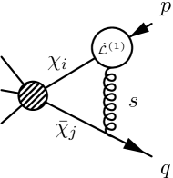
Figure 1: Soft loop with a single insertion of the sub-leading power Lagrangian $\hat{\cal L}^{(1)}_{\xi_{i}}$, that gives rise to mixing of the time-ordered product $J^{T1}$ into $J^{A1}$. The three lines on the left symbolize possible further collinear directions, not present in our example.

The gauge-invariant form (11) was obtained from the original SCET Lagrangian after a particular field redefinition. The original Lagrangian, which follows from the expansion of the QCD fields in the collinear and soft momentum region, reads [12]

$$\hat{\cal L}^{(1)}_{\xi_{i}}=\bar{\xi_{i}}\left(i\not{D}_{\perp i}\frac{1}{in_{i+}D_{i}}g_{s}\not{A}_{s\perp i}+g_{s}\not{A}_{s\perp i}\frac{1}{in_{i+}D_{i}}i\not{D}_{\perp i}+[(x_{\perp i}\partial)(g_{s}n_{i-}A_{s})]\right)\frac{n\hskip-4.49997pt/_{i+}}{2}\xi_{i}\,.$$ (13)

Here, (above) and below all soft fields $A_{s}$ without explicit argument are evaluated at $x_{i-}^{\mu}=\frac{1}{2}n_{i+}x\,n_{i-}^{\mu}$, and $iD_{i}=i\partial+g_{s}A_{i}(x)+\frac{1}{2}g_{s}n_{i-}A_{s}\,n_{i+}$ where $A_{i}$ is the collinear gauge field for direction $i$. In the following, we focus on the abelian case to avoid unnecessary complications, and then return to non-abelian gauge symmetry in Section 6. For the abelian case the field redefinition reads explicitly [13]

$$\xi_{i}\to(1+ig_{s}x_{\perp i}A_{s})\xi_{i}\,.$$ (14)

The difference between the Lagrangians (13) and (11) is given by the eom Lagrangian

$$\Delta{\cal L}^{(1)}_{\xi_{i}}\equiv\hat{\cal L}^{(1)}_{\xi_{i}}-{\cal L}^{(1)}_{\xi_{i}} = \bar{\xi_{i}}\left[ig_{s}x_{\perp i}A_{s},in_{i-}D_{i}+i\not{D}_{\perp i}\frac{1}{in_{i+}D_{i}}i\not{D}_{\perp i}\right]\frac{n\hskip-4.49997pt/_{i+}}{2}\xi_{i}$$ (15)

$$= \bar{\xi_{i}}\,ig_{s}x_{\perp i}A_{s}\frac{\delta S_{\xi_{i}}^{(0)}}{\delta\bar{\xi}_{i}}+{\rm h.c.}\,,$$

where

$$S_{\xi_{i}}^{(0)}=\int d^{d}x\,{\cal L}_{\xi_{i}}^{(0)},\quad{\cal L}_{\xi_{i}}^{(0)}=\bar{\xi_{i}}\left(in_{i-}D_{i}+i\not{D}_{\perp i}\frac{1}{in_{i+}D_{i}}i\not{D}_{\perp i}\right)\frac{n\hskip-4.49997pt/_{i+}}{2}\xi_{i}$$ (16)

is the leading-power action. The eom Lagrangian $\Delta{\cal L}^{(1)}_{\xi_{i}}$ does not contribute to on-shell matrix elements. For example, the diagram shown in Figure 1 is proportional to $(p^{2})^{-\epsilon}$ in $d$ dimensions. For the on-shell matrix element one performs the limit $p^{2}\to 0$ before taking the limit $\epsilon\to 0$. The rules of dimensional regularization then imply that $(p^{2})^{-\epsilon}\to 0$, in which case the eom Lagrangian gives rise to a scaleless integral that vanishes.

However, in order to extract the anomalous dimension from the UV divergences of the amplitude, one uses a small off-shellness of the external states. In practice, this means that one takes the limit $\epsilon\to 0$ first to extract the UV divergence, and then $p^{2}\to 0$, while the order of limits is opposite when computing genuine on-shell matrix elements. The limit $p^{2}\to 0$ must exist for the anomalous dimension to be well-defined as has indeed been found [14, 22, 23].

We now consider the same diagram as before, but with insertion of $\hat{\cal L}^{(1)}_{\xi_{i}}$ from (13), and find

$$2ig^{2}\,{\bf T}_{i}\cdot{\bf T}_{j}\,\overline{u}_{q}\Gamma v_{p}\,(n_{j+}q)(n_{i+}p)\,\mu^{2\epsilon}\!\int\frac{d^{d}k}{(2\pi)^{d}}\frac{1}{k^{2}\left(p^{2}-n_{i+}p\,n_{i-}k\right)^{2}\left(q^{2}+n_{j+}q\,n_{j-}k\right)}$$

$$\hskip 14.22636pt\times\left[-(n_{j-}p_{\perp i})\frac{p^{2}}{n_{i+}p}+\Big{\{}(n_{j-}p_{\perp i})(n_{i-}k)-(n_{i-}n_{j-})(p_{\perp i}k)\Big{\}}\right]$$

$$=\frac{\alpha_{s}}{\pi}\,{\bf T}_{i}\cdot{\bf T}_{j}\,\overline{u}_{q}\Gamma v_{p}\,\frac{n_{j-}\cdot p_{\perp i}}{(n_{i-}n_{j-})n_{i+}p}\left(\frac{-\mu^{2}s^{(0)}_{ij}}{p^{2}q^{2}}\right)^{\!\epsilon}\left(\frac{1}{\epsilon}+\mathcal{O}(\epsilon^{0})\right).$$ (17)

The last two terms in the curly bracket in the second line reproduce the amplitude (12) obtained with the SCET Lagrangian insertion (11). The first term is, however, different. Naively, it would not be expected to contribute in the on-shell limit $p^{2}\to 0$. However, the integral in the first line is proportional to $1/\epsilon\times 1/(p^{2})^{1+\epsilon}$ (see [23], Appendix B). Therefore this term survives in the limit $p^{2}\to 0$ and contributes to the anomalous dimension if the expansion in $\epsilon$ is done first as is required in this case.

The result (3) contains a UV divergent contribution proportional to the $J^{A1}$ operator. To cancel it, we need the counterterm

$$\delta Z^{kj}_{P_{i}Q_{i}}=\frac{\alpha_{s}}{2\pi\epsilon}\,{\bf T}_{k}\cdot{\bf T}_{j}\,\frac{n_{j-}^{\mu}\delta_{ki}}{(n_{k-}n_{j-})n_{i+}p_{i}}+(k\leftrightarrow j)\,.$$ (18)

In our specific example with $N=2$ we have $P_{i}=\bar{\chi}_{i^{\prime}}\Gamma J^{T1}_{i}$ and $Q_{i}=\bar{\chi}_{i^{\prime}}\Gamma J_{i}^{A1\,\mu}$ (where $i^{\prime}=2$ for $i=1$ and vice versa) and after summing over all contributions $kj=12,21$ according to (2.14) in [23], which gives a factor of two, we find that the counterterm (18) cancels the divergence in (3). The result holds also for the case of open spin and color indices, which is straightforward in color operator notation, and does not get modified in the non-abelian case (see Section 6). Furthermore, it can be generalized to more than two jets ($N>2$), the only change being that $P_{i}$ and $Q_{i}$ are given by the $N$-jet operators defined below (5). Finally, the counterterm (18) yields an additional contribution when matching to the corresponding QCD current, that is precisely of the form required to reproduce the IR divergences up to $\mathcal{O}(\lambda)$.

The counterterm (18) gives precisely the missing contribution (5) to the soft anomalous dimension. Hence we have shown that, contrary to conventional wisdom, the eom operator (15), which produces the first term in (3), mixes into physical operators. Moreover, it is the Lagrangian (13) rather than (11) that reproduces the IR divergences of the full QCD amplitude. This raises two fundamental questions: How is the KSZ theorem violated? What determines which Lagrangian or field representation of SCET is the one that correctly reproduces QCD in the IR, when employing an off-shell regulator to extract the anomalous dimension?

4 Violation of the Kluberg-Stern-Zuber theorem

The fact that the renormalization of an eom operator (the part of the time-ordered product $J_{i}^{T1}$ containing $\Delta{\cal L}^{(1)}_{\xi_{i}}$) requires to introduce a counterterm proportional to a physical operator (here $J^{A1\,\mu}_{i}$) contradicts the statement that eom operators do not mix into physical operators. In the following, we summarize and adapt to our case the main points of the proof of this statement [3], which we refer to as the KSZ theorem. We then show how one of the assumptions is violated in SCET.

Consider an action $S[\chi_{i}]$ that depends on a set of fields $\{\chi_{i}\}$. A general eom operator can be written as

$$\partial_{S}F(x)\equiv\int d^{d}y\,\frac{\delta S}{\delta\chi_{i}(y)}K_{i}(y,x)F(x)\,,$$ (19)

where $F[\chi_{i}](x)\equiv F(x)$ is a local operator (e.g $\chi_{1}^{2}$ or $\chi_{1}\partial^{\mu}\chi_{2}$), and $K_{i}(y,x)$ are arbitrary c-number kernels (e.g. $\delta^{(d)}(x-y)$ or $\partial_{\mu}\delta^{(d)}(x-y)$). A summation over all types of fields $i$ is implied. In the following we leave this summation implicit, e.g. $J\chi\equiv J_{i}\chi_{i}$. The generating functional is

$$Z[J,X,Y]=e^{i\,W[J,X,Y]}=\int{\cal D}\chi\,e^{iS+i\int_{x}(J\chi+X\partial_{S}F+YF)}\,,$$ (20)

where sources $X(x)$ and $Y(x)$ are introduced to generate single insertions of $\partial_{S}F$ and $F$, respectively, and ${\cal D}\chi$ encompasses the integration over all fields. We also use the shorthand $\int_{x}\equiv\int d^{d}x$.

By performing the field redefinition $\chi(y)\to\chi^{\prime}(y)=\chi(y)-\int_{x}K(y,x)F(x)X(x)$ and using ${\cal D}\chi={\cal D}\chi^{\prime}$ one finds $Z[J,X,0]=Z[J,0,\bar{Y}[J,X]]+{\cal O}(X^{2})$ where $\bar{Y}[J,X](x)=-\int_{y}J(y)K(y,x)X(x)$. After taking a functional derivative and setting $X=0$, this yields the Ward identity for eom operators,

$$\frac{\delta W}{\delta X(x)}\Big{|}_{X=Y=0}=-\int_{y}J(y)K(y,x)\frac{\delta W}{\delta Y(x)}\Big{|}_{X=Y=0}\,.$$ (21)

For the one particle irreducible (1PI) effective action (21) gives

$$\Gamma_{\partial_{S}F} = \int_{y}\left(\frac{\delta\Gamma}{\delta\chi(y)}K(y,x)\frac{\delta W}{\delta Y(x)}\right)\Big{|}_{X=Y=0}$$ (22)

$$= \int_{y}\left(\frac{\delta\Gamma}{\delta\chi(y)}\Big{|}_{X=Y=0}\right)K(y,x)\Gamma_{F}(x)\equiv\partial_{\Gamma}\Gamma_{F}\,.$$

This equation is still valid for arbitrary $\chi$, so we can generate relations for $n$-point, amputated, 1PI Green functions by taking derivatives with respect to $\chi$. Integrating over $x$ on both sides, assuming $K=K(y-x)$ (we depart from this choice later), and going to momentum space implies

$$\int_{x}\Gamma_{\partial_{S}F(x)}^{\rm 1PI}(p_{1},\dots,p_{n}) = \sum_{r=0}^{n}\sum_{\{i_{1},\dots,i_{r}\}\atop\subset\{1,\dots,n\}}\int_{p}\Gamma^{\rm 1PI}(p_{i_{1}},\dots,p_{i_{r}},p)$$ (23)

$$\times K(p)\times\Gamma_{F(p)}^{\rm 1PI}(p_{i_{r}+1},\dots,p_{i_{n}}),$$

where $\Gamma^{\rm 1PI}(p_{1},\dots,p_{n})$ are 1PI $n$-point functions, and $\Gamma_{\cal O}^{\rm 1PI}(p_{1},\dots,p_{n})$ are 1PI $n$-point functions with an insertion of ${\cal O}$. Diagrammatically this implies factorization of the $n$-point function with insertion of the eom operator (19) into a 1PI graph containing an insertion of $F$ and a usual 1PI graph without any insertion, as illustrated in Figure 2. The left diagram shows the left-hand side of (23) for $n=8$, and the right one shows one contribution to the right-hand side for $r=3$. The blobs may contain an arbitrary number of loops. As is apparent from Figure 2, the integration over $p$ does not count as a loop: for $\Gamma^{\rm 1PI}(p_{i_{1}},\dots,p_{i_{r}},p)=(2\pi)^{d}\delta^{(d)}(p_{i_{1}}+\cdots+p_{i_{r}}+p)\tilde{\Gamma}^{\rm 1PI}(p_{i_{1}},\dots,p_{i_{r}},p)$ the integration is removed and $p=-(p_{i_{1}}+\cdots+p_{i_{r}})$ is fixed by momentum conservation.

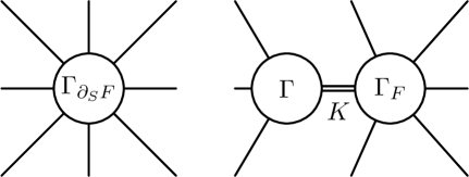
Figure 2: Diagrammatic representation of (23). See text for details.

To prove the KSZ theorem, we proceed recursively in the number of loops. We expand (22) in the number of loops,

$$\Gamma_{\partial_{S}F}^{(L)}=\sum_{\ell=0}^{L}\partial_{\Gamma^{(\ell)}}\Gamma_{F}^{(L-\ell)}$$ (24)

and we assume that counterterms have been added to the action to make all 1PI functions finite at loop order $0,\dots,L-1$. Then the remaining divergences at the $L$-loop order are

$$\Gamma_{\partial_{S}F}^{(L),\rm div}=\partial_{\Gamma^{(0)}}\Gamma_{F}^{(L),\rm div}+\partial_{\Gamma^{(L),\rm div}}\Gamma_{F}^{(0)}\,.$$ (25)

Further, we assume that $K\times F$ contains a suppression in the power-counting parameter $\lambda$ (or in general, by some EFT power counting parameter $1/\Lambda$). Then, $\Gamma$ has to contain at least one power less than $\Gamma_{\partial_{S}F}$. Therefore, we can assume (in an extra recursion in powers of $\lambda$, or $1/\Lambda$) that $\Gamma^{(L)}$ is already rendered finite. Hence, only the first term contributes, and $\Gamma^{(0)}=S$ implies that

$$\Gamma_{\partial_{S}F}^{(L),\rm div}=\partial_{S}\Gamma_{F}^{(L),\rm div}\,.$$ (26)

Consequently, we can remove the $L$-loop divergences by adding to the action a term of the form $\sum_{F^{\prime}}Z_{FF^{\prime}}^{(L)}\partial_{S}F^{\prime}$. Here $S$ already contains counterterms up to order $L-1$. If one assumes that $\Gamma_{F}^{(L),div}$ and $K(p)$ are polynomials in the momenta (i.e. local divergences), then $\partial_{S}\Gamma_{F}^{(L),div}$ is an eom operator. It follows that only eom operators $\partial_{S}F^{\prime}$ are required to renormalize 1PI Green functions with a single insertion of $\partial_{S}F$, which proves the theorem.

Now we return to the question of why the KSZ theorem is violated for the soft mixing computation in SCET. In the case of interest the relevant eom operator corresponds to $K^{\mu}(y,x)=-ix_{\perp i}^{\mu}\delta^{(d)}(y-x)$ and

$$F^{\mu}(x)=T\left\{J_{i}^{A0},g_{s}A_{s}^{\mu}(x_{i-})\xi_{i}(x)\right\}$$ (27)

(together with the corresponding hermitian-conjugated terms), which means that, due to the factor $x_{\perp i}^{\mu}$ in the kernel, a derivative of the momentum-space 1PI Green function appears in (23), which now reads

$$\int_{x}\Gamma_{\partial_{S}F(x)}^{\rm 1PI}(p_{1},\dots,p_{n}) = \sum_{r=0}^{n}\sum_{\{i_{1},\dots,i_{r}\}\atop\subset\{1,\dots,n\}}\int_{p}\Gamma^{\rm 1PI}(p_{i_{1}},\dots,p_{i_{r}},p)$$ (28)

$$\times\frac{\partial}{\partial p_{\perp i}^{\mu}}\Gamma_{F^{\mu}(p)}^{\rm 1PI}(p_{i_{r}+1},\dots,p_{i_{n}})\,.$$

In the example with two collinear directions $i$, $j$ discussed in the previous section, $n=2$, and the only contribution comes from $r=1$, because there is no one-point function generated by $\Gamma^{\rm 1PI}$. The above identity then takes the form

$$\int_{x}\Gamma_{\partial_{S}F(x)}^{\rm 1PI}(p,q) = \int_{\tilde{p}}\Gamma^{\rm 1PI}(p,\tilde{p})\frac{\partial}{\partial\tilde{p}_{\perp i}^{\mu}}\Gamma_{F^{\mu}(\tilde{p})}^{\rm 1PI}(q).$$ (29)

To obtain the contribution relevant to the example at order $\alpha_{s}$, we need to insert the two-point tree-level function $\Gamma^{\rm 1PI}_{\rm tree}(p,\tilde{p})$ and the one-point one-loop function with an insertion of (27), $\Gamma_{F^{\mu}(p)}^{\rm 1PI,1-loop}(q)$, whose explicit forms are

$$\Gamma^{\rm 1PI}_{\rm tree}(p,\tilde{p}) = \frac{p^{2}}{n_{i+}p}\,(2\pi)^{d}\delta^{(d)}(p-\tilde{p})\,,$$

$$\Gamma_{F^{\mu}(\tilde{p})}^{\rm 1PI,1-\rm loop}(q) = -\frac{\alpha_{s}}{4\pi}\frac{1}{\epsilon^{2}}\,{\bf T}_{i}\cdot{\bf T}_{j}\left(\frac{n_{i+}\tilde{p}n_{j+}q\,(n_{i-}n_{j-})\,\mu^{2}}{-2\tilde{p}^{2}q^{2}}\right)^{\!\epsilon}\frac{2n_{j-}^{\mu}}{(n_{i-}n_{j-})}\,.$$ (30)

The integral over $\tilde{p}$ is trivial in this case and after expanding in $\epsilon$ we find a divergent part that can only be renormalized by introducing a counterterm proportional to the physical operator $J_{i}^{A1\,\mu}$, in line with the previous explicit computation. Indeed, the divergent $1/\epsilon$ part of (29) takes the form

$$\int_{x}\Gamma_{\partial_{S}F(x)}^{\rm 1PI,div}(p,q)\propto\frac{p^{2}}{n_{i+}p}\times\frac{\partial}{\partial p_{\perp i}^{\mu}}\underbrace{\Gamma_{F^{\mu}(p)}^{\rm 1PI,div}(q)}_{\propto(p^{2})^{-\epsilon}/\epsilon^{2}}$$ (31)

at the one-loop order. The first factor $p^{2}$ on the right-hand side corresponds to the contribution from $\partial_{S}$ in $\Gamma_{\partial_{S}F}^{\rm div}=\partial_{S}\Gamma_{F}^{\rm div}$, that—in the familiar cases, such as QCD— would ensure that only eom counterterms are required to renormalize the eom operator. However, since in SCET $\Gamma_{F}^{\rm div}\propto\log(p^{2})/\epsilon$ and $K(p)\sim\partial/\partial p_{\perp}$ are not polynomials in the momenta, the assumption of locality in the KSZ proof is violated, and counterterms proportional to physical operators may be required. We conclude that the KSZ theorem is violated due to the momentum derivative coming from the $x_{\perp}^{\mu}$ term in the Lagrangian, which in turn arises from the multipole expansion, and because $\Gamma_{F}^{\rm div}$ has a logarithmic dependence on $p^{2}$ instead of polynomial dependence since in SCET double poles in $1/\epsilon$ appear already at one loop.

5 Uniqueness and preferred fields

The violation of the KSZ theorem raises the question, which eom operators should be included in the derivation of the SCET anomalous dimensions. For example, in the usual situation any multiple of $\Delta{\cal L}^{(1)}_{\xi_{i}}$ could be added to the Lagrangian. In SCET, however, while not affecting the bare on-shell matrix elements, this would change the anomalous dimension by an arbitrary amount. In other words, there exists a preferred set of SCET fields which gives the correct anomalous dimension and reproduces the IR singular behaviour of QCD. Apparently, the preferred set of fields is the one in which the Lagrangian takes the form (13), despite not being manifestly gauge-invariant.

The Lagrangian (13) is obtained from full QCD by separating fields into collinear and soft, and by performing the multipole expansion of the soft fields without using the equations of motion [12]. It therefore faithfully and directly reproduces the diagrammatic expansion in the method-of-region sense [35] of the QCD amplitudes in the collinear and soft regions on- or off-shell. The preferred set of fields is therefore these “original fields” that construct the soft-collinear expansion of the off-shell QCD amplitudes. Since the SCET Lagrangian is not renormalized in any order of perturbation theory [12], the corresponding Lagrangian can easily be constructed to any desired order in the expansion in $\lambda$.

To sum up this discussion, the violation of the KSZ theorem implies that indeed there is a preferred set of fields to compute the anomalous dimensions of power-suppressed $N$-jet operators in SCET, at least when the UV singularities are extracted by calculating the amplitudes with off-shell IR regulators, as is usually done. The fields are uniquely fixed by the requirement to reproduce the off-shell amplitudes of QCD at tree-level due to the non-renormalization of SCET. The mixing of the eom operators into physical operators generates additional counterterm vertices proportional to the physical operators that must be taken into account in SCET calculations (see Section 7 and Figure 4 below). However, once the counterterms and anomalous dimensions are determined, eom operators are no longer needed, field redefinition may be performed, and any Lagrangian (for instance, either (11) or (13)) obtained in this way can be used to compute on-shell amplitudes in SCET, since the insertion of eom operators into on-shell amplitudes gives scaleless integrals. Only the tree-level diagrams with the above-determined counterterm vertices are not scaleless, and must be included, in order to reproduce correctly the IR singularities of the full QCD amplitude.

6 Extension of soft mixing to the non-abelian case

It is quite cumbersome to write down the Lagrangian and eom terms in the “original fields” for the non-abelian theory including the Yang-Mills Lagrangian, and, in fact, this has never been done. In this section, we devise a method that side-steps this issue. It is enough to know the field redefinition that connects the fields in the gauge-invariant form of the Lagrangian to the “original fields”. Both the gauge-invariant Lagrangian and field redefinition can be constructed from [13]. This method allows us to efficiently compute the additional eom contributions to soft mixing, also at $\mathcal{O}(\lambda^{2})$ [32].

We discriminate between two sets of field variables for each collinear direction: the original collinear quark $\hat{\xi}$ and gluon $\hat{A}_{c}$ fields that transform under soft gauge transformations as

$$\hat{\xi}\to U_{s}(x)\hat{\xi},\quad\hat{A}_{c}\to U_{s}(x)\hat{A}_{c}U_{s}(x)^{\dagger}$$ (32)

and the redefined fields $\xi$ and $A_{c}$, which transform homogeneously in $\lambda$ as

$$\xi\to U_{s}(x_{-})\xi,\quad A_{c}\to U_{s}(x_{-})A_{c}U_{s}(x_{-})^{\dagger}\,.$$ (33)

For quantities expressed in terms of the fields $\xi$ and $A_{c}$ soft gauge invariance is manifest at every order in $\lambda$. When computing on-shell S-matrix elements, both sets of fields can be used. Indeed, the field operators are auxiliary quantities, and physical S-matrix elements do not depend on field redefinitions. Nevertheless, as seen above, this is not the case when keeping a (small) off-shellness on the external lines in order to extract UV divergences. We refer to these quantities as off-shell regulated S-matrix elements.

From the practical point of view, it is desirable to use the redefined fields, such that the sub-leading power Lagrangian as well as the $N$-jet operator basis, are manifestly gauge invariant at every order in $\lambda$ [13, 21]. On the other hand, to extract the anomalous dimension, the off-shell regulator requires the use of Green functions generated from the original fields. We now derive a relation that allows us to calculate the latter in terms of special Green functions of redefined fields.

We can express the original fields in terms of the redefined fields through relations of the form

$$\hat{\xi} = F[\xi,A_{c}]=\xi+\lambda F^{(1)}[\xi,A_{c}]+\lambda^{2}F^{(2)}[\xi,A_{c}]+{\cal O}(\lambda^{3})\,,$$

$$\hat{A}_{c} = G[\xi,A_{c}]=A_{c}+\lambda G^{(1)}[\xi,A_{c}]+\lambda^{2}G^{(2)}[\xi,A_{c}]+{\cal O}(\lambda^{3})\,,$$ (34)

where we keep $\lambda$ as a book-keeping parameter. Ref. [13] gives implicit all-order in $\lambda$ relations between the $\xi$, $A_{c}$ and $\hat{\xi}$, $\hat{A}_{c}$ fields in terms of a soft Wilson line from $x_{-}^{\mu}$ to $x^{\mu}$ and a collinear Wilson line. Expanding these relations we obtain

$$F^{(1)}[\xi,A_{c}] = ig_{s}x_{\perp}A_{s}(x_{-})\xi\,,$$

$$G^{(1)\mu}[\xi,A_{c}] = [ig_{s}x_{\perp}A_{s}(x_{-}),A_{c}^{\mu}]+\frac{1}{2}n_{+}^{\mu}\left(W_{c}x_{\perp}^{\nu}n_{-\rho}F_{s}^{\nu\rho}W_{c}^{\dagger}-x_{\perp}^{\nu}n_{-\rho}F_{s}^{\nu\rho}\right)\,.$$ (35)

The field redefinition for $n_{+}A_{c}$ is fixed only up to residual gauge transformation and the above relations hold only for a specific, non-covariant gauge choice. In practice, we want to use a covariant gauge fixing in the original fields to ensure that the SCET LSZ $Z$-factor of the collinear fields as well as the $\overline{\rm MS}$ field renormalization factor does not receive any $\mathcal{O}(\lambda)$ contribution at one-loop, such that the LSZ $Z$-factor remains the same with the above field redefinition. This choice allows to directly compare the on-shell Green functions computed with the original fields to those computed with the redefined fields. At leading power, this corresponds to the gauge fixing adopted in [23]. However, after expressing the gauge-fixing Lagrangian in terms of the new fields, new $\mathcal{O}(\lambda)$ collinear-soft gluon interactions appear. These do not contribute to diagrams with a single insertion of the $\mathcal{O}(\lambda)$ contribution to the gauge-fixing Lagrangian with one or several collinear external particles, as will be considered below. For the detailed discussion of gauge invariance and the construction of the field redefinition we therefore refer to [32].

We expand the full collinear Lagrangian in $\lambda$ in terms of the original fields, and alternatively in terms of the redefined fields,

$$\hat{\cal L}[\hat{\xi},\hat{A}_{c}]=\sum_{n}\lambda^{n}\hat{\cal L}^{(n)}[\hat{\xi},\hat{A}_{c}],\qquad{\cal L}[\xi,A_{c}]=\sum_{n}\lambda^{n}{\cal L}^{(n)}[\xi,A_{c}]\,.$$ (36)

The terms ${\cal L}^{(n)}$ are manifestly gauge invariant order by order in $\lambda$ [13]. Even though the individual terms differ, the sum over all terms satisfies ${\cal L}[\xi,A_{c}]=\hat{\cal L}[\hat{\xi},\hat{A}_{c}]$.

For computing the off-shell regulated S-matrix elements, we need to consider Green functions of the original fields. Taking the $\lambda$-derivative of the appropriate generating functional with respect to the book-keeping parameter, and then formally setting $\lambda=0$, generates the $\mathcal{O}(\lambda)$ time-ordered product insertion. Besides, we take functional derivatives with respect to the appropriate sources to generate the insertion of the current ${\cal J}$ and the fields in the Green function of interest. Expressing the generating functional in terms of either the original or the redefined fields gives

$$\langle 0|T\{{\cal J}(0)\,\left(i\int_{x}{\hat{\cal L}}^{(1)}\right)\,\hat{\xi}(p_{1})\cdots\hat{\xi}(p_{n})\}|0\rangle=\langle 0|T\{{\cal J}(0)\,\left(i\int_{x}{\cal L}^{(1)}\right)\,\xi(p_{1})\cdots\xi(p_{n})\}|0\rangle$$

$$+\sum_{r=1}^{n}\langle 0|T\{{\cal J}(0)\xi(p_{1})\cdots\xi(p_{r})\cdots\xi(p_{n})\}|0\rangle\Big{|}_{\xi(p_{r})\to F^{(1)}(p_{r})}\,.$$ (37)

This relation expresses the content of the Ward identity for eom operators. It can be trivially extended to Green functions with gluon fields, conjugated collinear quark fields as well as additional fields in other collinear directions.

The left-hand side corresponds to the Green function that must be used to extract the anomalous dimension. Instead, it is more efficient to use the sum of terms on the right. The first term after the equality sign corresponds to diagrams with a single insertion of the manifestly gauge-invariant Lagrangian ${\cal L}^{(1)}$, which vanishes [23]. The second line corresponds to replacing one of the fields that generate the external lines by the composite operator $F^{(1)}$. These terms yield the mixing of the time-ordered product into the $J^{A1}$ current. For Green functions with collinear gluons, one has to replace $F^{(1)}$ by $G^{(1)}$ for every gluon field appearing.

We now return to the explicit computation of mixing of the time-ordered products at $\mathcal{O}(\lambda)$ into the $J^{A1}$ currents, and generalize the previous treatment to the non-abelian case making use of the Ward identity (6). The Feynman rules for the contribution from the insertion of $F^{(1)}$ or $G^{(1)}$ for an external outgoing collinear antiquark or gluon, respectively, to the off-shell regulated S-matrix element are given by

$$\begin{array}[]{lll}\raisebox{-36.98857pt}{\includegraphics[width=89.90935pt]{feyn/F1}}&&ig_{s}t^{a}X_{\perp}^{\mu}\frac{p^{2}}{n_{+}p}\frac{\not{n}_{+}}{2}v_{p}^{c}\,,\end{array}$$ (38)

$$\begin{array}[]{lll}\raisebox{-36.98857pt}{\includegraphics[width=89.90935pt]{feyn/G1}}&&g_{s}f^{abc}p^{2}\left(X_{\perp}^{\mu}g^{\nu\rho}-\frac{1}{2}\frac{n_{+}^{\nu}n_{+}^{\rho}}{n_{+}p}X_{\perp}^{\lambda}n_{-}^{\sigma}(k_{\lambda}\delta^{\mu}_{\sigma}-k_{\sigma}\delta^{\mu}_{\lambda})\right)\epsilon_{\rho c}^{*}\,.\end{array}$$ (39)

Here the cross denotes the external line, that is multiplied with the inverse free propagator and the external spinor or polarization vector, respectively, as appropriate for the off-shell regulated S-matrix element. The symbol $X_{\perp}^{\mu}$ denotes the momentum-derivative on the momentum-conservation delta-function, and is defined as in (A.12) of [23].

Both vertices are proportional to $p^{2}$, i.e. they vanish in the on-shell limit unless this factor is cancelled by a factor $1/p^{2}$ coming from the diagram. This occurs for example in one particle reducible (1PR) diagrams with a loop in the external line, for which $F^{(1)}$ or $G^{(1)}$ are part of the loop. These are precisely the type of contributions that are cancelled by the corresponding LSZ $Z$-factor related to the “composite” operator used to generate the external states when computing on-shell matrix elements. In the present case, these contributions vanish because when closing the soft gluon loop on the same collinear direction, the leading-power soft interaction yields a factor of $n_{-}^{\mu}$, which vanishes when connecting the soft gluon to $F^{(1)}$ and $G^{(1)}$. This is in line with the observation that the $\mathcal{O}(\lambda)$ corrections to the LSZ Z-factor vanish in dimensional regularization and ensures that on-shell Green functions of the original or redefined fields are identical in covariant gauges.

Another possibility is to connect the soft gluon to another collinear direction. In this case, the momentum derivative contained in $X_{\perp}$ produces a soft loop which is non-vanishing, and contains a propagator with two powers as in (12), that can lead to the factor $1/p^{2}$, which cancels the $p^{2}$ from the vertex. This yields the contributions that we obtained before from the explicit insertion of the eom Lagrangian.

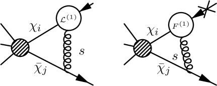
Figure 3: Diagrams that describe the mixing $\bar{\chi}_{j}J_{\chi_{i}}^{T1}\to\bar{\chi}_{j}[i\partial_{\perp i}^{\mu}\chi_{i}]$ according to the Ward identity (6).

The relevant diagrams for the mixing $\bar{\chi}_{j}J_{\chi_{i}}^{T1}\to\bar{\chi}_{j}[i\partial_{\perp i}^{\mu}\chi_{i}]$ are shown in Figure 3. The left diagram corresponds to the first line on right-hand side of (6) and it vanishes [23]. The right diagram contains the insertion of $F^{(1)}$, and yields the divergence that can be absorbed by a counterterm proportional to the $J^{A1}$ operator. The corresponding contribution to the soft anomalous dimension equals (5) obtained earlier. This confirms that the method developed in this section is equivalent to the explicit use of the Lagrangian with original fields, that is, it checks the Ward identity (6), and shows that the previous result (5) is also valid for the non-abelian case. Similarly, for the collinear gluon building block in the $i$ direction and a collinear quark in the other direction (that is, $j$ or $k$, whichever is different from $i$), which requires using $G^{(1)}$, we find

$$\gamma^{kj}_{P_{i}Q_{i}}=g_{\perp i}^{\rho\sigma}\,\frac{\alpha_{s}}{\pi}\,{\bf T}_{k}\cdot{\bf T}_{j}\,\frac{n_{j-}^{\mu}\delta_{ki}}{(n_{k-}n_{j-})n_{i+}p_{i}}+(k\leftrightarrow j)\,,$$ (40)

with $P_{i}=J^{A0}_{1}\ldots J^{T1}_{{\cal A}_{\perp i}^{\rho}}\ldots J^{A0}_{N}$ and $Q_{i}=J^{A0}_{1}\ldots J^{A1}_{[i\partial_{\perp i}^{\mu}{\cal A}_{\perp i}^{\sigma}]}\ldots J^{A0}_{N}$. In (40), we display explicitly the open Lorentz indices $\rho,\sigma,\mu$ of the gluon building blocks in the $i$ direction for clarity, but leave implicit all open Lorentz or Dirac indices in the other collinear directions. Altogether, $\gamma^{kj}_{P_{i}Q_{i}}$ is diagonal in all these indices (including the $i$, $k$ and $j$ direction), and (40) agrees with (5) when leaving also the indices of the building block for the $i$ direction implicit, that is, when suppressing the factor $g_{\perp i}^{\rho\sigma}$. Using this compact notation, we find that the anomalous dimension for the case of a gluon building block in both the $k$ and the $j$ directions has also a form identical to (5).

7 Collinear emission, mixing into B1 currents and divergent convolutions

To check the consistency of the above results we consider the on-shell amplitude with an additional transverse $i$-collinear gluon, $\langle\bar{q}(p_{1})q(q)g(p_{2})|J(0)|0\rangle$, in QCD and its representation in SCET. Here $J(0)=\bar{\psi}\,\Gamma\psi$ denotes a QCD quark-antiquark current, and $p_{1},p_{2}$ are the $i$-collinear momenta of the anti-quark and gluon. To simplify the notation, we restrict ourselves in this section to two collinear directions, $i$ and $j$, and assume that the power-suppression of the operator arises in the $i$-direction. Then, at $\mathcal{O}(\lambda)$, the collinear fields for the $j$-direction always consist of the single $\bar{\chi}_{j}$. We therefore simply write $J^{B1\,\mu}$ for $\bar{\chi}_{j}\Gamma J^{B1\,\mu}_{i}=\bar{\chi}_{j}\Gamma\mathcal{A}_{\perp i}^{\mu}\chi_{i}$. Similarly, $J^{A1\,\mu}$, $J^{T1}$ etc. are understood to contain the factor $\bar{\chi}_{j}\Gamma$.

We first restrict ourselves to the abelian terms and focus on divergent terms of the form $1/p^{2}\times 1/\epsilon$, where $p^{2}=(p_{1}+p_{2})^{2}$ is the virtuality of the collinear quark-gluon pair. We then find, as was the case for the amplitude without extra emission, that the sub-leading power eom Lagrangian $\Delta{\cal L}^{(1)}_{\xi_{i}}$ (15) vanishes when inserted into the on-shell amplitude, since the soft loop is scaleless. However, the counterterm $\delta Z_{J^{T1},\,J^{A1\,\mu}}$ (18) from mixing of $\Delta{\cal L}^{(1)}_{\xi_{i}}$ into the $J^{A1}$ operator contributes a $1/p^{2}\times 1/\epsilon$ pole from the one-particle reducible tree diagram with counterterm insertion. We find that this contribution is precisely what is required to reproduce the divergence of the full QCD amplitude in the limit $p^{2}\to 0$.

The SCET calculation of this amplitude at $\mathcal{O}(\lambda)$ includes a term of the form

$$\int_{0}^{1}dx\,C^{(A0,B1)}(x)\,\langle\bar{q}(q)q(p_{1})g(p_{2})|[\bar{\chi}_{j}\mathcal{A}_{\perp i}\chi_{i}](x)|0\rangle,$$ (41)

representing the convolution of the matrix element of a B1-type operator in momentum space with its hard QCD-to-SCET matching coefficient. The variable $x$ is the fraction of total $i$-collinear momentum carried by the gluon field in the operator. We find that the convolution of the tree-level coefficient function with the one-loop matrix element contributes to the above mentioned $1/p^{2}\times 1/\epsilon$ pole from the part of the coefficient function $C^{(A0,B1)}(x)$ which is proportional to $1/x$. However, when the convolution is performed after the matrix element is expanded in $\epsilon$, as would be the standard procedure, the convolution integral contains an unregulated divergence as $x\to 0$ and is ill-defined. Instead, the convolution must be done before the matrix element is expanded in $\epsilon$, in which case one finds agreement with the full QCD calculation, as stated above.

This observation has important implications for the soft mixing through the eom Lagrangian into B1 operators. To extract the anomalous dimension, we evaluate the matrix element of the time-ordered product operator in an external state with an additional, transverse $i$-collinear gluon as above, but now each leg carries a small off-shellness. We also return to the non-abelian theory. The relevant diagrams for soft mixing of $J^{T1}\to J^{B1\,\mu}=\bar{\chi}_{j}{\cal A}_{\perp i}^{\mu}\chi_{i}$ are shown in Figure 4. Diagrams with insertions of ${\cal L}^{(1)}$ are already omitted, because they vanish [23]. The insertions of the vertices $F^{(1)}$ and $G^{(1)}$ can appear only at the external lines according to the Ward identity (6). The second diagram in Figure 4 actually vanishes, because no collinear gauge field appears in $F^{(1)}$; see (38). The last diagram in Figure 4 is a 1PR tree-diagram with the insertion of the counterterm $\delta Z_{J^{T1},\,J^{A1\,\mu}}$ (18) at the operator vertex.

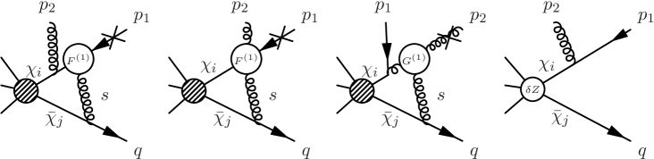
Figure 4: Diagrams that describe a potential mixing $J^{T1}\to\bar{\chi}_{j}{\cal A}_{\perp i}^{\mu}\chi_{i}$. Momenta are outgoing. We omit diagrams with insertions of ${\cal L}^{(1)}$, because they vanish.

The soft loop diagrams are no longer scaleless in the presence of the off-shell regulator. The $1/\epsilon$ pole of the soft contribution is proportional to $1/p^{2}$ i.e. it is non-local. It cannot be absorbed into a counterterm constructed from the $\mathcal{O}(\lambda)$ SCET operators, which are local except for the direction of the light-cone of collinear fields. It is also not possible to interpret the divergence as mixing of non-local time-ordered products into themselves as they have non-vanishing tree-level matrix elements only for external states with soft particles. It follows that contrary to the mixing $J^{T1}\to J^{A1\,\mu}=\bar{\chi}_{j}i\partial_{\perp}^{\mu}\chi_{i}$ it is not possible to define consistently the corresponding mixing into the B1-operator $\bar{\chi}_{j}\mathcal{A}_{\perp i}^{\mu}\chi_{i}$.

A related problem appears, however, for collinear loops. While the mixing of the B1 operator into itself is well-defined, and has been computed in [22] (see also [28, 29] for related computation in heavy-quark physics), some of the pole parts of the collinear contribution to the off-shell regulated matrix element are given by the convolution of the anomalous dimension with the tree-level matching coefficient similar to (41), which is again divergent. However, when the convolution is performed in $d$ dimensions before expanding the collinear loop integral in $\epsilon$, it generates a $1/\epsilon\times 1/p^{2}$ term, which exactly cancels the non-local divergence from the soft loops. Note that a similar cancellation of non-local $1/\epsilon\times\ln p^{2}$ poles between collinear and soft loops already appears in the computation of the one-loop cusp anomalous dimension (4) at leading power. In that case, however, the cancellation appears within the anomalous dimension of the A0 operator alone, while at next-to-leading power the cancellation would have to happen between different entries of the anomalous dimension matrix, each of which is separately ill-defined.

To solve both problems, that is, to construct a well-defined anomalous dimension matrix including a consistent treatment of the divergent convolution, we modify the basis of $\mathcal{O}(\lambda)$ SCET objects. We first define the “singular” B1 operator $J^{B1s\,\mu}$,

$$J^{B1s\,\mu}(t_{i},t_{j}) = \bar{\chi}_{j}(t_{j}n_{j+})\Gamma\left[\frac{1}{in_{i+}\partial}{\cal A}_{\perp i}^{\mu}(t_{i}n_{i+})\right]\chi_{i}(t_{i}n_{i+})\,.$$ (42)

Both building blocks in the $i$-collinear direction are evaluated at the same position $t_{i}$. The inverse derivative, which operates only inside the square bracket, translates into a factor $1/x$, the momentum fraction carried by the gluon building block, such that the operator itself, and hence its anomalous dimension, absorbs the singular endpoint behaviour of the matching coefficient of the standard B1-type operator, when the momentum of the gluon becomes soft. We then trade the objects $J^{A1\,\mu}$, $J^{B1\,\mu}$ and $J^{T1}$ for

$$J^{A1\,\mu},\quad J^{B1\,\mu}_{\rm reg}\,,\quad\check{J}\equiv J^{T1}+\frac{2n_{j-}^{\mu}}{n_{j-}n_{i-}}J^{B1s}_{\mu},$$ (43)

where the “regular” B1 operator is defined by analogy with the “$+$ distribution” as

$$J_{\rm reg}^{B1\,\mu}(x)=\lim_{\eta\to 0^{+}}\left[\theta(x-\eta)J^{B1\,\mu}(x)-\eta\delta(x-\eta)\int_{\eta}^{1}dz\frac{J^{B1\,\mu}(z)}{z}\right]\,.$$ (44)

The limit $\eta\to 0^{+}$ should be taken after the convolution integral with the coefficient function over $x$ is evaluated. The effect of the subtraction is to precisely remove the $1/x$ term from the coefficient function since this part is already included in the singular B1 operator. The operator $\check{J}$ is constructed in such a way that the non-local $1/\epsilon$ pole cancels in the sum of the time-ordered product and singular B1-operator term. The issue of a divergent convolution does not arise here since the singular B1 operator has the $i$-collinear fields at the same position. The originally divergent convolution is implicitly part of the operator, hence performed in $d$ dimensions, and the divergence subtracted by renormalization. Several consistency requirements must be satisfied to make this construction valid.

First, the two terms added together to $\check{J}$ must have the same divergence and the same hard matching coefficients to all orders in perturbation theory, so that $\check{J}$ renormalizes as a single object. Since the time-ordered product operator $J^{T1}$ inherits its evolution from the LP A0-operator, the singular B1-operator must have the same anomalous dimension and coefficient function as $J^{A0}$. We have seen that this holds for the tree-level matching coefficients by construction and we checked at the one-loop level that the anomalous dimension for $\check{J}\to\check{J}$ mixing indeed agrees with the one of the leading-power current $J^{A0}$. In fact, the combination $\check{J}$ of time-ordered product and singular B1 operator is reparameterization invariant and, hence, should stay intact to all orders.

Second, the anomalous dimension for the mixing of $J^{B1s}\to J^{B1}_{\rm reg}(y)$ must be finite as $y\to 0$. We find, for the operator with contracted colour indices ($C_{F}=4/3,C_{A}=3$),

$$\gamma_{J^{B1s\,\mu},J^{B1\,\nu}_{\rm reg\,\alpha\beta}(y)}=\frac{\alpha_{s}}{4\pi}\frac{1}{n_{i+}(p_{1}+p_{2})}\left(\Gamma\left[(C_{F}-C_{A}/2)\,\gamma_{\perp i}^{\mu}\gamma_{\perp i}^{\nu}\,\frac{\ln(\bar{y})}{y}+C_{F}\gamma_{\perp i}^{\nu}\gamma_{\perp i}^{\mu}\right]\right)_{\alpha\beta}\,,$$ (45)

which is indeed finite as $y\to 0$, and thus the mixing terms in the ADM for the new building block $\check{J}$ are

$$\gamma_{\check{J},J^{A1\,\nu}} = \gamma_{J^{T1},J^{A1\,\nu}}\,,$$

$$\gamma_{\check{J},J_{\rm reg\,\alpha\beta}^{B1\,\nu}(y)} = \frac{2n_{j-}^{\mu}}{n_{j-}n_{i-}}\gamma_{J^{B1s\,\mu},J_{\rm reg\,\alpha\beta}^{B1\,\nu}(y)}\,,$$ (46)

where we used that $J^{B1s}$ does not mix into $J^{A1}$ and that $J^{T1}$ does not mix into $J^{B1}_{\rm reg}$. The operator $J_{\rm reg}^{B1}(x)$ is renormalized by the same kernel as the unregularized $J^{B1}(x)$ operator [22, 23]. This completes the mixing of $\mathcal{O}(\lambda)$ quark-antiquark (+ gluon) currents including the soft mixing from eom operators and the renormalization of divergent convolutions.

Third, and finally, the coefficient function of the unregularized B1 operator must not be more singular than $1/x$ as $x\to 0$, and in particular, must not contain $1/x\times\ln^{n}x$ at higher orders, since this would invalidate the subtraction (44) in the definition of the regular operator. That is, to all orders in $\alpha_{s}$, we must have $C^{B1}(x)=c(\alpha_{s})/x+\mbox{less singular terms}$.

The appearance of a divergent convolution with the hard coefficient is a manifestation of the breakdown of naive soft-collinear factorization in SCET. Indeed, the $1/x$ behaviour of the tree-level B1-operator matching coefficient appears when the gluon in the operator, assumed to be collinear, becomes soft. In full QCD, the $1/x$ behaviour originates from the coupling of the $i$-collinear gluon to another collinear direction. This explains why the cancellation of the non-local pole occurs between the singular part of the B1-type operator and the time-ordered product with soft gluon exchange between two collinear directions, and why only the sum $\check{J}$ is well-defined from the renormalization perspective. Divergent convolution integrals are familiar in SCET, but usually appear in the breakdown of factorization between modes of the same virtuality but different light-cone momentum or rapidity [36], resulting in a divergence that cannot be regulated dimensionally. Here, however, we encounter divergent convolutions with hard matching coefficients, related to the breakdown of factorization between regions of different virtuality, collinear and soft, which are regulated dimensionally. A similar problem has appeared first to our knowledge in the computation of electromagnetic corrections to $B_{s}\to\mu^{+}\mu^{-}$ [30], where the computation was performed with an additional analytic regulator, since modes with different and equal virtuality are required, as well as in [31] in a context with collinear and soft modes with different virtuality, which resembles more closely the situation discussed here. However, in both cases the endpoint divergence arose in a diagram with soft fermion exchange, whereas here it appears in a more standard context of soft-gluon exchange. We suspect that such divergences are generic for SCET beyond LP, at least as soon as the collinear directions are no longer back-to-back, which is always the case when more than two jets are involved. It remains an open problem whether divergent convolutions in factorization formulas between functions of different virtuality can always be renormalized by the introducing singular and regular multi-jet operators as in the simplest case discussed above.

8 Summary

We investigated the mixing of time-ordered products of SCET $N$-jet operators with power-suppressed terms in the Lagrangian into $N$-jet operators and we found that the KSZ theorem is violated. That is, soft-collinear interaction Lagrangians that are equivalent by the equation of motion yield different anomalous dimensions for the $N$-jet operators. The violation is caused by the peculiar structure of interactions in SCET, involving the multipole expansion of soft fields that generates $x$-dependent terms in the Lagrangian, resulting in momentum derivatives, and by the fact that the anomalous dimension must capture a double $1/\epsilon^{2}$ pole per loop, which is related to the cusp anomalous dimension. The eom terms do not affect SCET on-shell matrix elements once the relevant counterterms have been obtained. However, the mixing of eom operators into physical operators implies that there is a preferred field representation for the anomalous dimension calculation, which is the one that reproduces correctly the IR singularities of QCD.

Notwithstanding this surprising result, SCET is a sensible EFT, since the eom terms and preferred set of fields are easily identified. Unlike other EFTs, the SCET Lagrangian is fixed completely by tree-level matching and no new operators are induced to any order in $\alpha_{s}$. Thus, even though eom operators mix into physical operators, only a finite number of such counterterms appears at a given order in the $\lambda$ expansion. The Lagrangian that produces the correct anomalous dimension is the one that reproduces the off-shell tree-level amplitudes in QCD. The additional soft mixing of eom operators must be added to the one-loop anomalous dimension computed in [22, 23], as illustrated here for the case of $\mathcal{O}(\lambda)$ power-suppressed quark-antiquark operators.

We confirmed that the additional soft mixing from eom Lagrangians into A1-type operators is actually required to reproduce IR divergences of QCD in SCET in more general kinematic situations. We checked this by performing the on-shell matching for A1 currents in the non-back-to-back kinematic configuration with non-vanishing transverse momenta with respect to the collinear direction axis. In addition, we checked that at one loop, the soft region of QCD with off-shell regulator is exactly reproduced at the integrand level by the sum of SCET physical and eom terms. We also find that the soft mixing is consistent with reparameterization invariance of SCET and is in fact required by Lorentz invariance of the cusp anomalous dimension.

Extending the investigation to the mixing into B-type currents revealed divergent convolution integrals of the hard matching coefficient with the SCET matrix element for operators with more than one collinear field in a given direction. Such divergences have been observed before in a few cases involving soft fermion exchange [30, 31], but here they appear in a comparatively standard situation with soft gluons. They therefore seem to be generic and impede a consistent definition of the anomalous dimension matrix without further considerations. We proposed a split of the B-type operator into a singular and a regular part, such that the renormalization of the singular operator includes the consistent renormalization of the endpoint divergence of the convolution integral. The construction is supported by reparameterization invariance and passes the available consistency checks. The generality of the proposed solution should be further studied. The issue is of paramount importance for NLP resummation beyond the leading logarithms.

Our analysis was formulated in the position-space formulation of SCET [12, 13], but we expect the same results in the label formulation [10, 11]. Although there are no $x_{\perp}^{\mu}$ factors (hence momentum derivatives) in the label SCET Lagrangian, the propagator denominators with higher powers also appear in this formalism, as well as, evidently, the soft-collinear double $1/\epsilon^{2}$ poles. Momentum derivatives and $x$-factors also appear in the Lagrangian of potential non-relativistic field theory [37, 38]. Nevertheless, we do not expect a violation of the KSZ theorem in this case, despite the structural similarity of the $\mathcal{O}(\lambda)$ dipole interaction of the soft gauge field. In non-relativistic systems, the multipole expansion is performed in the spatial dimensions, rather than the transverse directions. After performing the integration over the time component of loop momentum, one obtains ordinary Feynman integrals in three dimensions, which can be regulated dimensionally. As a result one finds single poles in $\epsilon$ only and no convolution integrals that could be divergent.

Acknowledgements

We thank A. Manohar for valuable comments. This work was supported in part by the BMBF grant No. 05H18WOCA1.

References

- [1] W. S. Deans and J. A. Dixon, Theory of Gauge Invariant Operators: Their Renormalization and S Matrix Elements, Phys. Rev. D18 (1978) 1113–1126.
- [2] H. D. Politzer, Power Corrections at Short Distances, Nucl. Phys. B172 (1980) 349–382.
- [3] H. Kluberg-Stern and J. B. Zuber, Renormalization of Nonabelian Gauge Theories in a Background Field Gauge. 2. Gauge Invariant Operators, Phys. Rev. D12 (1975) 3159–3180.
- [4] S. D. Joglekar and B. W. Lee, General Theory of Renormalization of Gauge Invariant Operators, Annals Phys. 97 (1976) 160.
- [5] D. Espriu, Renormalization of Gauge Invariant Operators and the Axial Anomaly, Phys. Rev. D28 (1983) 349.
- [6] J. C. Collins and R. J. Scalise, The Renormalization of composite operators in Yang-Mills theories using general covariant gauge, Phys. Rev. D50 (1994) 4117–4136, [hep-ph/9403231].
- [7] A. V. Manohar, Introduction to Effective Field Theories, in Les Houches summer school: EFT in Particle Physics and Cosmology Les Houches, Chamonix Valley, France, July 3-28, 2017, 2018, 1804.05863.
- [8] J. C. Criado and M. Pérez-Victoria, Field redefinitions in effective theories at higher orders, JHEP 03 (2019) 038, [1811.09413].
- [9] P. Gambino, M. Gorbahn and U. Haisch, Anomalous dimension matrix for radiative and rare semileptonic B decays up to three loops, Nucl. Phys. B673 (2003) 238–262, [hep-ph/0306079].
- [10] C. W. Bauer, S. Fleming, D. Pirjol and I. W. Stewart, An Effective field theory for collinear and soft gluons: Heavy to light decays, Phys. Rev. D63 (2001) 114020, [hep-ph/0011336].
- [11] C. W. Bauer, D. Pirjol and I. W. Stewart, Soft collinear factorization in effective field theory, Phys. Rev. D65 (2002) 054022, [hep-ph/0109045].
- [12] M. Beneke, A. P. Chapovsky, M. Diehl and T. Feldmann, Soft collinear effective theory and heavy to light currents beyond leading power, Nucl. Phys. B643 (2002) 431–476, [hep-ph/0206152].
- [13] M. Beneke and T. Feldmann, Multipole expanded soft collinear effective theory with non-abelian gauge symmetry, Phys. Lett. B553 (2003) 267–276, [hep-ph/0211358].
- [14] T. Becher and M. Neubert, Infrared singularities of scattering amplitudes in perturbative QCD, Phys. Rev. Lett. 102 (2009) 162001, [0901.0722].
- [15] M. Beneke, F. Campanario, T. Mannel and B. D. Pecjak, Power corrections to decay spectra in the ‘shape-function’ region, JHEP 06 (2005) 071, [hep-ph/0411395].
- [16] A. J. Larkoski, D. Neill and I. W. Stewart, Soft Theorems from Effective Field Theory, JHEP 06 (2015) 077, [1412.3108].
- [17] S. M. Freedman and R. Goerke, Renormalization of Subleading Dijet Operators in Soft-Collinear Effective Theory, Phys. Rev. D90 (2014) 114010, [1408.6240].
- [18] D. W. Kolodrubetz, I. Moult and I. W. Stewart, Building Blocks for Subleading Helicity Operators, JHEP 05 (2016) 139, [1601.02607].
- [19] I. Feige, D. W. Kolodrubetz, I. Moult and I. W. Stewart, A Complete Basis of Helicity Operators for Subleading Factorization, JHEP 11 (2017) 142, [1703.03411].
- [20] I. Moult, I. W. Stewart and G. Vita, A subleading operator basis and matching for gg H, JHEP 07 (2017) 067, [1703.03408].
- [21] M. Beneke, M. Garny, R. Szafron and J. Wang, Subleading-power -jet operators and the LBK amplitude in SCET, in 13th International Symposium on Radiative Corrections: Application of Quantum Field Theory to Phenomenology (RADCOR 2017) St. Gilgen, Austria, September 24-29, 2017, 2017, 1712.07462.
- [22] M. Beneke, M. Garny, R. Szafron and J. Wang, Anomalous dimension of subleading-power N-jet operators, JHEP 03 (2018) 001, [1712.04416].
- [23] M. Beneke, M. Garny, R. Szafron and J. Wang, Anomalous dimension of subleading-power -jet operators. Part II, JHEP 11 (2018) 112, [1808.04742].
- [24] I. Moult, I. W. Stewart, G. Vita and H. X. Zhu, First Subleading Power Resummation for Event Shapes, JHEP 08 (2018) 013, [1804.04665].
- [25] M. Beneke, A. Broggio, M. Garny, S. Jaskiewicz, R. Szafron, L. Vernazza et al., Leading-logarithmic threshold resummation of the Drell-Yan process at next-to-leading power, JHEP 03 (2019) 043, [1809.10631].
- [26] M. A. Ebert, I. Moult, I. W. Stewart, F. J. Tackmann, G. Vita and H. X. Zhu, Subleading power rapidity divergences and power corrections for qT, JHEP 04 (2019) 123, [1812.08189].
- [27] M. Beneke, Y. Kiyo and D. s. Yang, Loop corrections to subleading heavy quark currents in SCET, Nucl. Phys. B692 (2004) 232–248, [hep-ph/0402241].
- [28] R. J. Hill, T. Becher, S. J. Lee and M. Neubert, Sudakov resummation for subleading SCET currents and heavy-to-light form-factors, JHEP 07 (2004) 081, [hep-ph/0404217].
- [29] M. Beneke and D. Yang, Heavy-to-light B meson form-factors at large recoil energy: Spectator-scattering corrections, Nucl. Phys. B736 (2006) 34–81, [hep-ph/0508250].
- [30] M. Beneke, C. Bobeth and R. Szafron, Enhanced electromagnetic correction to the rare -meson decay , Phys. Rev. Lett. 120 (2018) 011801, [1708.09152].
- [31] S. Alte, M. König and M. Neubert, Effective Field Theory after a New-Physics Discovery, JHEP 08 (2018) 095, [1806.01278].
- [32] M. Beneke, M. Garny, R. Szafron and J. Wang, in preparation.
- [33] S. Catani, The Singular behavior of QCD amplitudes at two loop order, Phys. Lett. B427 (1998) 161–171, [hep-ph/9802439].
- [34] A. V. Manohar, T. Mehen, D. Pirjol and I. W. Stewart, Reparameterization invariance for collinear operators, Phys. Lett. B539 (2002) 59–66, [hep-ph/0204229].
- [35] M. Beneke and V. A. Smirnov, Asymptotic expansion of Feynman integrals near threshold, Nucl. Phys. B522 (1998) 321–344, [hep-ph/9711391].
- [36] M. Beneke and T. Feldmann, Factorization of heavy to light form-factors in soft collinear effective theory, Nucl. Phys. B685 (2004) 249–296, [hep-ph/0311335].
- [37] A. Pineda and J. Soto, Effective field theory for ultrasoft momenta in NRQCD and NRQED, Nucl. Phys. Proc. Suppl. 64 (1998) 428–432, [hep-ph/9707481].
- [38] M. Beneke, Perturbative heavy quark - anti-quark systems, in Proceedings of the 8th International Symposium on Heavy Flavor Physics (Heavy Flavors 8), 1999, hep-ph/9911490.