Magnetization Dynamics in 1D Chains of Ferromagnetic Nanoparticles Coupled with Dipolar Interactions: Blocking Temperature

Abstract

There is so far no clear-cut experimental analysis that can determine whether dipole-dipole interactions enhance or reduce the blocking temperature $T_{B}$ of nanoparticle assemblies. It seems that the samples play a central role in the problem and therefore, their geometry should most likely be the key factor in this issue. Yet, in a previous work, Jönsson and Garcia-Palacios did investigate theoretically this problem in a weak-interaction limit and without the presence of an external DC field. Based on symmetry arguments they reached the conclusion that the variation of the relaxation rate is monotonous. In the presence of an external magnetic field we show that these arguments may no longer hold depending on the experimental geometry. Therefore, the aim of this paper is to evaluate the variation of $T_{B}$ for a model system consisting of a chain of ferromagnetic nanoparticles coupled with long-range dipolar interaction with two different geometries. Rather than addressing a quantitative analysis, we focus on the qualitative variation of $T_{B}$ as a function of the interparticle distance $a$ and of the external field $h$. The two following situations are investigated: a linear chain with a longitudinal axial anisotropy in a longitudinal DC field and a linear chain with a longitudinal axial anisotropy in a transverse field.

I Introduction

The magnetization dynamics in magnetic nanoparticles (MNP) assemblies is the corner stone of many physical observables such as the dynamical susceptibility, the magnetic resonance and many others. However, having a direct access to these observables does not guarantee that one is able to disentangle the collective effects from the intrinsic properties of the isolated nanoparticles. The competition between these two effects might indeed impair the true picture that one should have of the long range interaction physics in such complex systems (Z. Sabsabi, F. Vernay, O. Iglesias, H. Kachkachi, 2013; Vernay et al., 2014). For this reason, and thanks to the long-standing endeavor that has been devoted to the study of MNP assemblies, it is desirable to first deal with the relatively simple and ordered low-dimensional systems. Quasi bi-dimensional assemblies are nowadays well controlled by chemists, see e.g. (Toulemon et al., 2011; Pauly et al., 2011, 2012), and 1D chains of magnetic nanoparticles have been investigated for more than 30 years in magnetotactic bacteria (Mann, 1985) with a recent revival of interest (Bazylinski and Frankel, 2004; Charilaou et al., 2011; Myrovali et al., 2016) due to their potential applications. In order to clearly highlight the effect of dipole-dipole interactions (DDI) on the dynamics of MNP assembly, we tackle the problem by determining semi-analytically the behavior of the blocking temperature $T_{B}$ in 1D chains of MNP, which requires the calculation of the relaxation rate of the chain.

For non-interacting systems, the problem has been addressed in many works, including the pioneering works of Néel, Brown and Aharoni (Néel, 1950; Brown, 1963; Aharoni, 1969). Here, our system consists of a chain of $\mathcal{N}$ ferromagnetic nanoparticles, with a restriction to monodisperse assemblies of monodomain MNP. The latter are represented by a single macrospin, $\bm{m}_{i}=m{\bf S}_{i}=n\mbox{$\mu$}_{B}{\bf S}_{i}$, with a uniaxial anisotropy. All anisotropy axes are parallel and aligned along the chain direction ${\bf e}_{z}$. We apply to the system an external DC magnetic field ${\bf H}$ that can be either longitudinal (along ${\bf e}_{z}$) or transverse (${\bf e}_{\perp}$). The two situations are presented in Fig 1.

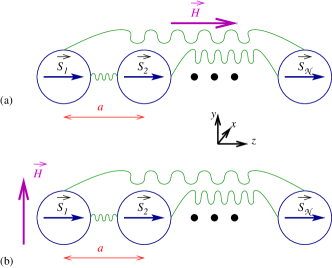
Figure 1: 1D chain of $\mathcal{N}$ magnetic nanoparticles. All magnetic nanoparticles are interacting via long range dipolar interaction depicted in green, each nanoparticle has a uniaxial anisotropy axis along $z$. Two situations are considered: (a) a longitudinal field with respect to the chain and to the anisotropy axis, or (b) a transverse field.

The aim of this study is to investigate the variation of $T_{B}$ as a function of the interparticle distance $a$ and the applied external dc field $H$. A naive approach would be to take an Arrhenius law giving the relaxation time as

$$\tau=\tau_{D}e^{\frac{\Delta\mathcal{E}}{k_{B}T}},$$ (1)

where $\Delta\mathcal{E}$ represents the energy barrier between the two potential wells and $\tau_{D}$ the diffusion time. The maximum blocking temperature is then defined with respect to the measuring timescale through the expression:

$$\tau_{{\rm mes}}=\tau_{D}e^{\frac{\Delta\mathcal{E}}{k_{B}T_{B}}}\ \Rightarrow T_{B}\propto\frac{\Delta\mathcal{E}}{k_{B}}.$$ (2)

We thus see that we first need to compute the variation of the energy barrier $\Delta\mathcal{E}\left(a,H\right)$ in the presence of a weak dipolar field. However, this simple approach suffers a major drawback: by focusing only on the barrier, one neglects the dynamics in the wells whilst Jönsson and García-Palacios showed that the latter plays an essential role in the determination of the blocking temperature (Jönsson and García-Palacios, 2001, 2001). In order to take this dynamics into account, we compute the relaxation rate $\Gamma$ in the presence of weak dipolar interactions, in the limit of intermediate to high damping using Langer’s theory (Langer, 1968; J.S. Langer, Statistical theory of the decay of metastable states, 1969). A similar approach was used by Braun for chains with exchange couplings (Braun, 1994) and is generalized here to take account of the specificity of the long range nature of the dipolar interaction (Vernay et al., 2014).

The paper is organized as follows: our model is introduced in Section II and we summarize the procedure to compute the relaxation rate by following Langer’s approach. The relaxation rate in the longitudinal field case is presented in details in Section III, while the computation for the transverse field case is done more briefly in Section IV. Our results are disclosed in Section V; we show in particular the behavior of the relaxation rate as a function of the field or the reduced energy barrier for different strengths of the DDI. We also provide a detailed discussion of the behavior of the blocking temperature in 1D MNP chains and interpret our results with the help of a simple analytical formula. The paper closes with a conclusion and outlook.

II Presentation of the model

The total energy of the chain is given by the addition of the anisotropy energy, the Zeeman energy and the dipole-dipole interaction (DDI) energy :

$$E=E_{{\rm anis}}+E_{{\rm Zeeman}}+E_{{\rm ddi}}$$ (3)

where

$$E_{{\rm anis}}=-\sum_{i=1}^{\mathcal{N}}KV\left(S_{i}^{z}\right)^{2}$$

$$E_{{\rm Zeeman}}=-\sum_{i=1}^{\mathcal{N}}{\bf H}\cdot\bm{m}_{i}$$

$$E_{{\rm ddi}} =-\frac{\mu_{0}}{4\pi}\frac{m^{2}}{a^{3}}\sum_{i=1}^{\mathcal{N}}\sum_{i<j}{\bf S}_{i}\mathcal{\bm{D}}_{ij}{\bf S}_{j}$$

with

$$\mathcal{\bm{D}}_{ij}=\frac{3\cdot{\bf e}_{ij}\ {\bf e}_{ij}\cdot-1}{r_{ij}^{3}},\quad r_{ij}=\left\|{\bf r}_{i}-{\bf r}_{j}\right\|,{\bf e}_{ij}=\frac{{\bf r}_{ij}}{r_{ij}}.$$

The total energy can be measured in units of $2KV$ (anisotropy energy), i.e. $\mathcal{E}=E/\left(2KV\right)$. Accordingly, we define the dimensionless physical parameters

$$h\equiv\frac{H}{H_{a}};\quad\xi\equiv\frac{\mu_{0}}{4\pi}\frac{m^{2}/a^{3}}{2KV}$$ (4)

but keep the anisotropy parameter $k=1$ so as to be able to track the anisotropy contribution in the subsequent developments. Consequently, we write

$$\mathcal{E}=\sum_{i}^{\mathcal{N}}\mathcal{E}_{i}=-\frac{k}{2}\sum_{i=1}^{\mathcal{N}}S_{i,z}^{2}-\sum_{i=1}^{\mathcal{N}}\bm{h}\cdot{\bf S}_{i}-\xi\sum_{i=1}^{\mathcal{N}}\sum_{i<j}{\bf S}_{i}\mathcal{\bm{D}}_{ij}{\bf S}_{j}.$$ (5)

The estimation of the relaxation rate for an interacting chain of nanoparticles may be relatively complicated to compute analytically because of the discrete sums. However, in the case of a chain, the lattice sum is straightforward to compute. We introduce the local coordinates for each spin $\left(\theta_{i},\varphi_{i}\right)$, such that $S_{i,z}\equiv\cos\theta_{i}$. We also define the compact notation $V_{ij}\equiv V\left(\bm{r}_{i}-\bm{r}_{j}\right)=1/\left\|\bm{r}_{i}-\bm{r}_{j}\right\|^{3}$ such that, owing to the symmetry with respect to rotations about the chain’s axis ($z$), we write the local energy as follows

$$\begin{array}[]{lll}\mathcal{E}_{i}&=&-\bm{h}\cdot\bm{S}_{i}-\frac{k}{2}S_{i,z}^{2}\\ \\ &-&\xi{\displaystyle\sum_{j\neq i}}V_{ij}\left[2S_{i,z}S_{j,z}-{\displaystyle\sum_{\alpha=x,y}}S_{i,\alpha}S_{j,\alpha}\right]\end{array}$$ (6)

and the total energy then reads

$$\begin{array}[]{lll}\mathcal{E}&=&-{\displaystyle\sum_{\alpha,i}}h^{\alpha}\;S_{i,\alpha}-\frac{k}{2}{\displaystyle\sum_{i}}S_{i,z}^{2}\\ \\ &-&\xi{\displaystyle\sum_{i,j\neq i}}\left[2S_{i,z}S_{jz}-{\displaystyle\sum_{\alpha=x,y}}S_{i,\alpha}S_{j,\alpha}\right].\end{array}$$ (10)

In the intermediate-to-high damping limit, the relaxation rate $\Gamma$ for an elementary process, i.e. an escape from a metastable state (m) to a state of lower energy, through a saddle point (s), can be calculated with the help of Langer’s theory (Langer, 1968; J.S. Langer, Statistical theory of the decay of metastable states, 1969). $\Gamma$ can be put into the following compact form (Kachkachi, H., 2003)

$$\Gamma=\frac{\left|\kappa\right|}{2\pi}\frac{\mathcal{Z}_{s}}{\mathcal{Z}_{m}},$$ (11)

where $\kappa$ represents the attempt frequency to cross the barrier, $\mathcal{Z}_{s}$ and $\mathcal{Z}_{m}$ are the partition functions at, respectively, the saddle point (s) and the metastable state (m). The explicit evaluation of Eq. (11) thus requires the analytical expression of the energy in the vicinity of the stable state and the saddle point.

III Longitudinal case $\boldsymbol{h}=h\boldsymbol{e}_{z}$

III.1 Energy barrier in the continuous limit in the longitudinal case

In order to compute the energy barrier we need to determine the saddle point. For this we compute the functional derivative $\delta\mathcal{E}_{i}/\delta S_{i,\alpha},\ \alpha=x,y,z$. The two transverse components (i.e. $\alpha=x,y$) yield the constraints:

$$\sum_{j}V_{ij}S_{j}^{\alpha=x,y}=0.$$

This is consistent with the fact that the problem is symmetric with respect to the $z$-axis. The longitudinal component $S_{z}$ contains the most relevant information about the energy barrier:

$$S_{i,z}=-\frac{h}{k}-4\frac{\xi}{k}\sum_{j}V_{ij}S_{j,z}$$ (12)

which can be self-consistently solved leading to the following result (to first order in $\xi$)

$$S_{i,z}^{\left(s\right)}=\cos\theta_{i}^{\left(s\right)}=-\frac{h}{k}\left[1-4\frac{\xi I_{i}}{k}\right],$$ (13)

with $I_{i}=\sum_{j}V_{ij}$ and where $\left(s\right)$ refers to the saddle point. We have checked that for chains of more than 20 particles, the sum $I_{i}$ is nearly constant along the chain with a maximum deviation at the edges of less than 5%. This implies that the lattice sum $I$ can be considered as independent of the site at which it is computed. Its limit is given by the Riemann zeta function $\zeta\left(3\right)\approx 1.202$. Henceforth, in a first approximation we consider chains that are sufficiently long to neglect edge effects, such that $I_{i}=I$ and consequently $\theta_{i}^{\left(s\right)}=\theta_{s}$. Substituting $S_{i,z}^{\left(s\right)}$ from Eq. (13) back into Eq. (6) yields

$$\mathcal{E}_{s\parallel}^{\left(0\right)}\left(r\right)=\frac{h^{2}}{2k}\left(1-4\frac{\xi I}{k}\right).$$ (14)

The energy at the (meta)stable state is gained by inserting $S_{i,z}^{\left(\pm\right)}=\pm 1$ into Eq. (6), such that the energy barrier $\Delta\mathcal{E}_{\pm}$ with respect to the (meta)stable state, $\mathcal{E}_{\pm}^{\left(0\right)}=\pm h-\frac{k}{2}-2\xi I$ is given by

$$\Delta\mathcal{E}_{\pm}^{\parallel}=\frac{k}{2}\left(1\pm\frac{h}{k}\right)^{2}+2\xi I\left(1-\frac{h^{2}}{k^{2}}\right)$$ (15)

where the $\pm$ sign refers to the relative orientation of the field with respect to the magnetic moments.

III.2 Evaluation of the partition functions

As is inherent to Langer’s approach, the expression of the partition functions in the vicinity of the saddle point and metastable state are obtained by performing a second-order expansion of the energy. For this purpose, it is easier to rewrite the equation of the energy in Eq. (6) in spherical coordinates $(\theta,\varphi)$. By definition of the extrema the first order derivative will not contribute to the expansion once evaluated thereat.

The second-order expansion around the saddle point then reads

$$\mathcal{E}_{s}^{\parallel}\simeq\mathcal{E}_{s\parallel}^{(0)}+\frac{1}{2}\left.\frac{\partial^{2}\mathcal{E}}{\partial\theta^{2}}\right|_{\theta_{s}}\left(\theta-\theta_{s}\right)^{2}.$$

Inserting the value of $\cos\theta_{s}$ obtained in Eq. (13) in the expression of the second derivative and keeping only the linear terms in $\xi$, leads to

$$\mathcal{E}_{s}^{\parallel}\simeq\mathcal{E}_{s\parallel}^{\left(0\right)}+\frac{1}{2}\underbrace{k\left(\frac{h^{2}}{k^{2}}-1\right)\left[1+\frac{8\frac{h^{2}}{k^{2}}\frac{\xi I}{k}}{1-\frac{h^{2}}{k^{2}}}\right]}_{=-\lambda_{t}<0}\left(\theta-\theta_{s}\right)^{2}.$$ (16)

If the chain is sufficiently long we may neglect the edge effects and assume that the deviation induced by the dipolar field is nearly constant over the whole chain. Hence, the partition function at the saddle point can be factorized and the partition function per spin then reads

$$\mathcal{Z}_{s,\parallel}=2\pi e^{-\beta\mathcal{E}_{s\parallel}^{\left(0\right)}}\sin\theta_{s}{\displaystyle\int}_{-\infty}^{+\infty}e^{-\beta\frac{\lambda_{t}}{2}\delta^{2}}d\delta$$

which can be computed and then expanded in terms of $\xi$

$$\mathcal{Z}_{s,\parallel}=\left(2\pi\right)^{3/2}\sqrt{\frac{k_{B}T}{k}}\ e^{-\beta\mathcal{E}_{s\parallel}^{\left(0\right)}}.$$ (17)

To first order, the dipolar field is only present because it shifts the energy of the saddle point by hardening the anisotropy. In the absence of $\xi$ in Eq. (17), one recovers the standard expression for a single spin with a uniaxial anisotropy.

Let us now compute $\mathcal{Z}_{-}$, the partition function near the metastable state. Since there is a rotational invariance around the $(Oz)$ axis, this part is easier to compute by using the Cartesian coordinates

$$\left\{\begin{array}[]{ccc}S_{z}^{2}&=&1-S_{x}^{2}-S_{y}^{2}\\ \\ S_{z}&\simeq&-1+\frac{1}{2}S_{x}^{2}+\frac{1}{2}S_{y}^{2}\end{array}\right.$$

hence, the energy around the metastable point may be written as

$$\begin{array}[]{lll}\mathcal{E}_{-}&\simeq&\underbrace{\left[-\frac{k}{2}+h-2\xi I\right]}_{=\mathcal{E}_{-}^{(0)}}\\ \\ &+&\underbrace{k\frac{1-h/k}{2}\left[1+\frac{4\xi I/k}{1-h/k}\right]}_{=\mu}\left(S_{x}^{2}+S_{y}^{2}\right).\end{array}$$

Therefore the partition function is given by

$$\begin{array}[]{lll}\mathcal{Z}_{-}&=&e^{-\beta\mathcal{E}_{-}^{\left(0\right)}}\left({\displaystyle\int_{-\infty}^{+\infty}}e^{-\beta\mu x^{2}}dx\right)^{2}\\ \\ &=&e^{-\beta\mathcal{E}_{-}^{\left(0\right)}}\frac{2\pi k_{B}T}{k\left(1-\frac{h}{k}\right)\left[1+\frac{4\xi I/k}{1-h/k}\right]}.\end{array}$$ (18)

From Eqs. (17) and (18), we obtain the ratio $\mathcal{Z}_{s,\parallel}/\mathcal{Z}_{-}$

$$\frac{\mathcal{Z}_{s,\parallel}}{\mathcal{Z}_{-}}=\sqrt{\frac{2\pi k}{k_{B}T}}\ e^{-\beta\Delta\mathcal{E}_{-}^{\parallel}}\ \left(1-\frac{h}{k}\right)\left[1+\frac{4\xi I/k}{1-\frac{h}{k}}\right]$$ (19)

where the energy barrier $\Delta\mathcal{E}_{-}$ is given by Eq. (15).

III.3 Attempt frequency

In order to complete the calculation of the relaxation rate of Eq. (11), we still have to compute the attempt frequency $\kappa$. This is given by the first nonzero negative eigenvalue of the transfer matrix. For computing it we proceed by writing the Landau-Lifshitz equation in spherical coordinates

$$\left\{\begin{array}[]{lcl}\dot{\theta}&=&-\frac{1}{\sin\theta}\partial_{\varphi}\mathcal{E}-\alpha\partial_{\theta}\mathcal{E},\\ \\ \dot{\varphi}&=&-\frac{\alpha}{\sin\theta}\partial_{\varphi}\mathcal{E}+\partial_{\theta}\mathcal{E}\end{array}\right.$$ (20)

where $\alpha$ is the damping parameter. We then make the expansion of the coordinates $\left(\theta,\varphi\right)$ around the saddle point $\left(\theta_{s},\varphi_{s}\right)$, i.e. $\theta\simeq\theta_{s}+t,\varphi\simeq\varphi_{s}+p$ and next expand the energy to second order (call the result $\mathcal{E}_{s}^{\left(2\right)}$) in $t,p$ upon which the Landau-Lifshitz equation becomes

$$\left\{\begin{array}[]{lcl}\overset{\cdot}{t}&=&-\partial_{p}\mathcal{E}_{s}^{\left(2\right)}-\alpha\partial_{t}\mathcal{E}_{s}^{\left(2\right)},\\ \\ \dot{p}&=&-\alpha\partial_{p}\mathcal{E}_{s}^{\left(2\right)}+\partial_{t}\mathcal{E}_{s}^{\left(2\right)}.\end{array}\right.$$

The two equations above can be recast into the following matrix form (using the notation $\eta_{i}=\left(t,p\right)$)

$$\partial_{t}\eta_{i}=\sum_{j}M_{ij}\partial_{\eta_{j}}\mathcal{E}_{s}^{\left(2\right)}.$$

Close to the saddle point, the energy may be expressed as $\mathcal{E}_{s}=\mathcal{E}_{s}^{\left(0\right)}+\frac{1}{2}\lambda_{t}t^{2}+\frac{1}{2}\lambda_{f}f^{2}$. In the present case, we have $\lambda_{f}=0$ and $\lambda{}_{t}$ is defined in Eq. (16). Hence, the eigenvalue of the resulting matrix leads to

$$\left|\kappa\right|=\alpha k\left(1-\frac{h^{2}}{k^{2}}\right)\left[1+\frac{8\frac{h^{2}}{k^{2}}\frac{\xi I}{k}}{1-\frac{h^{2}}{k^{2}}}\right].$$ (21)

III.4 Relaxation rate in the longitudinal case

The result in Eq. (21) and the ratio in Eq. (19) are used in Eq. (11) to compute the relaxation rate in longitudinal field, that is

$$\begin{array}[]{lll}\Gamma_{-\to s}&=&\alpha k^{3/2}\sqrt{\frac{\beta}{2\pi}}\left(1-\frac{h^{2}}{k^{2}}\right)\left(1-\frac{h}{k}\right)\\ \\ &\times&\left[1+\frac{8\frac{h^{2}}{k^{2}}\frac{\xi I}{k}}{1-\frac{h^{2}}{k^{2}}}\right]\left[1+\frac{4\xi I/k}{1-\frac{h}{k}}\right]e^{-\beta\Delta\mathcal{E}_{-}^{\parallel}}.\end{array}$$ (22)

By simply performing the change $h\to-h$, one can deduce the rate $\Gamma_{+\to s}$

$$\begin{array}[]{lll}\Gamma_{+\to s}&=&\alpha k^{3/2}\sqrt{\frac{\beta}{2\pi}}\left(1-\frac{h^{2}}{k^{2}}\right)\left(1+\frac{h}{k}\right)\\ \\ &\times&\left[1+\frac{8\frac{h^{2}}{k^{2}}\frac{\xi I}{k}}{1-\frac{h^{2}}{k^{2}}}\right]\left[1+\frac{4\xi I/k}{1+\frac{h}{k}}\right]e^{-\beta\Delta\mathcal{E}_{+}^{\parallel}}.\end{array}$$ (23)

Adding up these two equations renders the total relaxation rate of the chain’s magnetic moment

$$\begin{array}[]{lll}\Gamma_{\parallel}&=&\alpha k^{3/2}\sqrt{\frac{\beta}{2\pi}}\left(1-\frac{h^{2}}{k^{2}}\right)\\ \\ &\times&\left\{\left(1+\frac{h}{k}\right)\left[1+\frac{4\left(1-\frac{h}{k}+2\frac{h^{2}}{k^{2}}\right)\frac{\xi I}{k}}{1-\frac{h^{2}}{k^{2}}}\right]\ e^{-\beta\Delta\mathcal{E}_{+}^{\parallel}}\right.\\ \\ &+&\left.\left(1-\frac{h}{k}\right)\left[1+\frac{4\left(1+\frac{h}{k}+2\frac{h^{2}}{k^{2}}\right)\frac{\xi I}{k}}{1-\frac{h^{2}}{k^{2}}}\right]\ e^{-\beta\Delta\mathcal{E}_{-}^{\parallel}}\right\}.\end{array}$$ (24)

It can readily be checked that setting $\xi\to 0$ in this expression recovers the Néel-Brown result (Aharoni, 1969).

Eq. (24) shows that the energy at the saddle point changes due to the dipolar interaction as well as the external magnetic field. The concomitant presence of the two contributions leads to the additional cross term $\propto h^{2}\xi I$. In contrast, even in the absence of the DC field, the energies of the two minima are lowered by the same amount $2\xi I$ due to the dipolar interaction. This variation can be absorbed in the definition of the anisotropy constant $k$ by introducing the renormalized anisotropy constant $k^{\prime}=k\left(1+\frac{4\xi I}{k}\right).$ This means that the chain of interacting MNP would behave as a macrospin with effective uniaxial anisotropy of constant $k^{\prime}$ with easy axis along the chain.

IV Transverse field

The external magnetic field is now normal to the chain axis and the uniaxial anisotropy; we choose $\bm{h}=h\bm{e}_{x}$. The relaxation rate for the transverse field is then obtained by following the same procedure as described in detail in the previous section.

The energy in the continuum limit now reads

$$\begin{array}[]{lll}\mathcal{E}_{i}&=&-hS_{i,x}-\frac{k}{2}S_{i,z}^{2}\\ \\ &-&\xi{\displaystyle\sum_{j\neq i}}V_{ij}\left[2S_{i,z}S_{j,z}-{\displaystyle\sum_{\alpha=x,y}}S_{i,\alpha}S_{j,\alpha}\right],\end{array}$$ (25)

and can be re-expressed in spherical coordinates as it is more convenient for finding the extrema. The derivative with respect to $\varphi_{i}$ yields the following equation

$$h\sin\varphi_{i}-2\xi\sum_{j\neq i}V_{ij}\sin\theta_{j}\sin\left(\varphi_{i}-\varphi_{j}\right)=0.$$

Since the magnetic field is applied along the $x$ axis and the anisotropy is along the $z$ axis, the effective field is necessarily in the $xz$ plane and thereby we may simply set the azimuthal angle to zero, i.e. $\varphi_{i}=0$. Therefore, we derive the following simplified equation for the polar angle $\theta_{i}$

$$\begin{array}[]{lll}0&=&\cos\theta_{i}\left[-h+k\sin\theta_{i}\right]\\ \\ &+&2\xi{\displaystyle\sum_{j\neq i}}V_{ij}\left\{2\cos\theta_{j}\sin\theta_{i}+\sin\theta_{j}\cos\theta_{i}\right\}\end{array}$$ . (29)

This equation may be solved perturbatively and to first order in $\xi$ it yields the position of the saddle point $\theta_{s}$ and the minimum $\theta_{m}$

$$\left\{\begin{array}[]{lll}\theta_{s}&=&\frac{\pi}{2},\\ \\ \theta_{m}&=&\frac{h}{k}\left[1-\frac{6\xi I}{k}\right].\end{array}\right.$$ (30)

Next, we can evaluate the energy at these two points leading to $\mathcal{E}_{s\perp}^{\left(0\right)}=-h+\xi I$ and $\mathcal{E}_{m}^{\left(0\right)}=-\frac{k}{2}-\frac{h^{2}}{2k}-2\xi I\left[1-\frac{3}{2}\frac{h^{2}}{k^{2}}\right]$, and infer from the latter the energy barrier

$$\Delta\mathcal{E}^{\perp}=\mathcal{E}_{s\perp}^{\left(0\right)}-\mathcal{E}_{m}^{\left(0\right)}=\frac{k}{2}\left(1-\frac{h}{k}\right)^{2}+3\xi I\left(1-\frac{h^{2}}{k^{2}}\right).$$ (31)

Since the addition of the external magnetic field now explicitly breaks the rotational symmetry around the $z$-axis, the expansion of the energy in the vicinity of the saddle point and the metastable state contains a term in $\varphi$,

$$\begin{array}[]{lll}\mathcal{E}_{s}^{\perp}&\simeq&\mathcal{E}_{s\perp}^{\left(0\right)}+\frac{1}{2}\left[h-2\xi I\right]\left(\varphi-\varphi_{s}\right)^{2}\\ &+&\frac{1}{2}\left[-k+h-2\xi I\right]\left(\theta-\theta_{s}\right)^{2},\\ \\ \mathcal{E}_{m}&\simeq&\mathcal{E}_{m}^{\left(0\right)}+\frac{1}{2}\frac{h^{2}}{k}\left[1-\frac{8\xi I}{k}\right]\left(\varphi-\varphi_{s}\right)^{2}\\ &+&\frac{k}{2}\left[\left(1-\frac{h^{2}}{k^{2}}\right)+\frac{4\xi I}{k}\left(1+3\frac{h^{2}}{k^{2}}\right)\right]\left(\theta-\theta_{s}\right)^{2}.\end{array}$$ (32)

From this the partition function is obtained at the saddle point

$$\mathcal{Z}_{s,\perp}=\frac{2\pi k_{B}T}{k\sqrt{\frac{h}{k}\left(1-\frac{h}{k}\right)}}e^{-\beta\mathcal{E}_{s\perp}^{\left(0\right)}}\left(1+\frac{\xi I}{h}\frac{k-2h}{k-h}\right)$$ (33)

and at the minimum (metastable state)

$$\mathcal{Z}_{m}=\frac{2\pi k_{B}T}{k\sqrt{1-\frac{h^{2}}{k^{2}}}}e^{-\beta\mathcal{E}_{m}^{\left(0\right)}}\left(1-\frac{4\xi I}{k}\frac{k^{2}+h^{2}}{k^{2}-h^{2}}\right).$$ (34)

Hence, to first order in the dipolar interaction ($\xi$), their ratio reads

$$\begin{array}[]{lll}\frac{\mathcal{Z}_{s,\perp}}{\mathcal{Z}_{m}}&=&\sqrt{\frac{1-\frac{h^{2}}{k^{2}}}{\frac{h}{k}\left(1-\frac{h}{k}\right)}}e^{-\beta\Delta\mathcal{E}^{\perp}}\\ \\ &\times&\left[1+\xi I\frac{1+3\frac{h}{k}-2\left(\frac{h}{k}\right)^{2}+4\left(\frac{h}{k}\right)^{3}}{\frac{h}{k}\left(1-\frac{h^{2}}{k^{2}}\right)}\right].\end{array}$$ (35)

Similarly to what was done in subsection III.3, the expression of the energy in the vicinity of the saddle point given in Eq. (32), leads to the transition matrix and the attempt frequency is obtained upon diagonalizing the latter. This yields

$$\begin{array}[]{lll}\kappa&=&\frac{k}{2}\left[\alpha\left(1-\frac{2h}{k}\right)+2\sqrt{\frac{h}{k}\left(1-\frac{h}{k}\right)+\frac{\alpha^{2}}{4}}\right]\\ \\ &+&\xi I\left[2\alpha-\frac{1-\frac{2h}{k}}{\sqrt{\frac{h}{k}\left(1-\frac{h}{k}\right)+\frac{\alpha^{2}}{4}}}\right];\end{array}$$ (36)

which can symbolically written as $\kappa=\kappa^{\left(0\right)}+\xi I\kappa^{\left(1\right)}=\kappa^{\left(0\right)}\left(1+\xi I\frac{\kappa^{\left(1\right)}}{\kappa^{\left(0\right)}}\right)$, where $\kappa^{\left(0\right)}$ is the result for the single spin problem in a transverse field (D.A. Garanin, E.C. Kennedy, D.S.F. Crothers, and W.T. Coffey, 1999). By collecting the results of Eqs. (35) and (36) and inserting them into Eq. (11) we obtain the expression of the relaxation rate in a transverse field

$$\begin{array}[]{lll}\Gamma_{\perp}&=&\frac{\kappa^{\left(0\right)}}{2\pi}\sqrt{\frac{1-\frac{h^{2}}{k^{2}}}{\frac{h}{k}\left(1-\frac{h}{k}\right)}}e^{-\beta\Delta\mathcal{E}^{\perp}}\\ \\ &\times&\left[1+\xi I\left(\frac{1+3\frac{h}{k}-2\left(\frac{h}{k}\right)^{2}+4\left(\frac{h}{k}\right)^{3}}{\frac{h}{k}\left(1-\frac{h^{2}}{k^{2}}\right)}+\frac{\kappa^{\left(1\right)}}{\kappa^{\left(0\right)}}\right)\right].\end{array}$$ (37)

It can be readily checked that upon setting $\xi=0$, one recovers the relaxation rate of an isolated spin (D.A. Garanin, E.C. Kennedy, D.S.F. Crothers, and W.T. Coffey, 1999).

V Discussion of the results

Let us now consider a chain of monodisperse iron-cobalt particles with a radius $R=4\ {\rm nm}$, an effective uniaxial anisotropy $K=4.5\times 10^{4}\ {\rm J/m^{3}}$, and $M_{s}=1.162\times 10^{6}{\rm A/m}$. The reduced anisotropy barrier with respect to thermal energy is given by

$$\sigma=\frac{KV}{k_{B}T},$$ (38)

and is relatively large $\sigma\left(300{\rm K}\right)\simeq 3$ at room temperature. The free diffusion time $\tau_{D}$, defined by

$$\tau_{D}=\frac{M_{s}}{2\alpha\gamma_{g}K},$$ (39)

where $\gamma_{g}$ is the gyromagnetic ratio. With these specific parameters and for intermediate-to-high damping (namely $1\lesssim\alpha\lesssim 10$) $\tau_{D}$ varies between $7\times 10^{-11}{\rm s}$ and $7\times 10^{-12}{\rm s}$. As already mentioned earlier, the chain is assumed to be long enough so as to neglect the edge effects. We have checked that this assumption becomes valid when the chain consists of more than 20 nanoparticles.

V.1 Relaxation rate $\Gamma$

In the expressions of the longitudinal and transverse relaxation rates given in Eqs. (24) and (37), using the respective energy barriers in (15) and (31), we see that the arguments of the exponential functions are primarily governed by the zero field energy barrier $\sigma=KV/k_{B}T$. Besides, if we inspect more closely these two arguments for $h\to 0$, we realize that taking the interparticle dipolar interaction into account is equivalent to doing a renormalization of the anisotropy. For a 1D chain, the dipolar field can indeed only be along the chain and thus it merely brings an additional rigidity to the magnetic system. This implies that the relaxation rate decreases as the dipolar interaction increases. This can be checked in Figs. 2-(a) and (b) where the logarithm of the relaxation rate is plotted against the field for different dipolar strengths $\xi$.

(a)

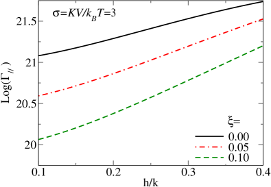
(b)

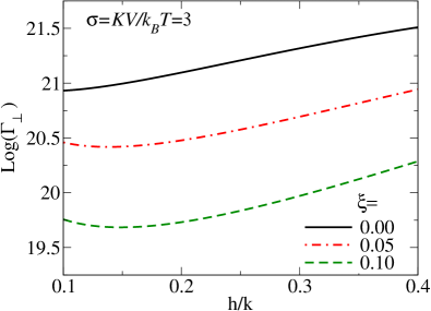
Figure 2: Relaxation rate as a function of the external dc field for different values of the dipolar interaction $\xi$. The damping parameter is $\alpha=1$ for both sets.

The relaxation rate $\Gamma_{\parallel}$ is mostly given by $\exp\left(-\beta\Delta\mathcal{E}_{-}^{\parallel}\right)$ and its prefactor as $h$ increases. In the prefactor, $\xi$ is coupled to $h$ only via positive terms. This implies a monotonic behavior of $\log\left(\Gamma_{\parallel}\right)$ as a function of $h$.

In contrast, the prefactor of the relaxation rate $\Gamma_{\perp}$ in transverse field has a more involved expression which is a non monotonic function of $h$. As a consequence, and as it can be seen in Fig. 2-(b), we observe a competition between the external and the dipolar fields. For finite $\xi$, the relaxation rate first decreases at low fields and then increases when $h$ overcomes the additional rigidity brought in by $\xi$.

(a)

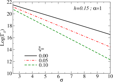
(b)

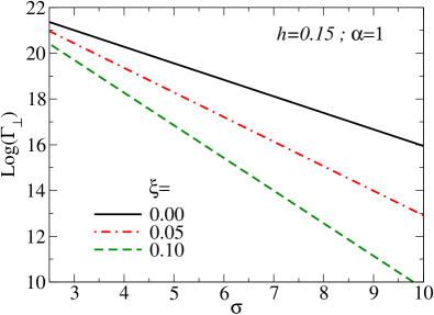
Figure 3: Relaxation rate as a function of $\sigma=KV/k_{B}T$ for different values of the dipolar interaction $\xi$ and for a finite external field $\frac{h}{k}=0.15$.

When the anisotropy barrier $\sigma$ becomes large enough, say $\sigma\gtrsim 2.5$, the behavior of $\log\left(\Gamma_{\parallel}\right)$ and $\log\left(\Gamma_{\perp}\right)$ as a function of $\sigma$ is nearly linear as seen in Figs. 3–(a) and (b). The effect of the dipolar field is mainly to increase the (anisotropy) rigidity as explained earlier and is more pronounced in the transverse field case. This can be understood by inspecting the expressions of the energy barriers given by Eqs. (15) and (31): the numerical prefactor in front of $\xi$ is larger in $\Delta\mathcal{E}_{\perp}$.

V.2 Blocking temperature $T_{B}$

The blocking temperature is obtained by solving Eq. (2) for an experiment specific time $\tau_{{\rm mes}}$. In the case of magnetic nanoparticles, the characterization of magnetic properties can be achieved through SQUID experiments with a typical measuring time $\tau_{{\rm SQUID}}=10^{-2}{\rm s}$.

(a)

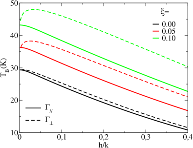
(b)

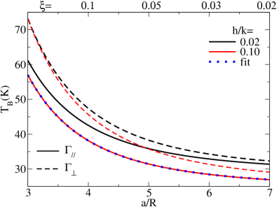
Figure 4: (a) $T_{B}$ as a function of the reduced external field $h$ for different values of $\xi$. (b) $T_{B}$ as a function of the interparticle distance $a$ (in units of the particle radius $R$) for different values of the applied field $h$. For both panels $\alpha=1$, the dashed lines represent the transverse field case, the continuous line shows the longitudinal field case. The measuring time is typical of SQUID experiment $\tau_{{\rm SQUID}}=10^{-2}{\rm s}$.

The blocking temperature $T_{B}$ is plotted in Fig. 4-(a) as a function of the external field for various dipolar strengths. When $h\to 0$, one sees that $T_{B}^{\perp}$ and $T_{B}^{\parallel}$ nearly coincide as expected. In the longitudinal case, the blocking temperature is a decreasing function of $h$. Indeed, in this case, as already stated earlier, the prefactor of the relaxation rate does not play much of a role as it is a monotonic function of $h$ (for low field and low $\xi$). Hence, the addition of the external field for a finite $\xi$ is seen in the energy barrier and facilitates the magnetization reversal by making more pronounced saddle points. All in all, this results in a reduced $T_{B}$ as $h$ increases.

The situation in transverse field is more subtle: it involves both the energy barrier and the prefactor of the relaxation rate. At a relatively high field, the physics is governed by the energy barrier which is strongly reduced, and hence $T_{B}$ decreases by increasing $h$. In the low-field regime $h/k<0.05$, $h$ couples to $\xi$ and the competition that occurs between the dipolar (longitudinal) field and the external (transverse) field leads to a nonmonotonic behavior of $T_{B}$: as $h$ increases, $T_{B}^{\perp}$ first increases, and then decreases when a critical value of the transverse field is reached.

Fig. 4-(b) shows the blocking temperature against the interparticle distance $a$ for two different values of the external field. The interparticle distance range has been chosen so that we remain in the limit $\xi\ll 1$, indeed even for $a/R=3$, we have $\xi\approx 0.232$. The behavior of $T_{B}^{\perp}$ and $T_{B}^{\parallel}$ is in line with the previous observations. Indeed, knowing that $\xi\propto a^{-3}$, we see that if $a$ is increased the effective magnetic anisotropy of the chain is reduced and the blocking temperature is lowered since the energy barrier can be more easily overcome by the magnetic moments.

Indeed, for both Figs 4-(a) and (b) the overall behavior of $T_{B}$ can be understood if one simply uses the Arrhenius law since then Eq. (2) can be easily solved to obtain (to the leading order in $h/k$)

$$T_{B}=\frac{1}{\log\left(\frac{\tau_{{\rm mes}}}{\tau_{D}}\right)}\left\{\begin{array}[]{lll}\frac{k}{2}\left(1-2\frac{h}{k}\right)+2\xi I(\bm{r})&,&\ \parallel\\ \\ \frac{k}{2}\left(1-2\frac{h}{k}\right)+3\xi I(\bm{r})&,&\ \perp\end{array}\right.$$ (40)

Eq. (40) correctly accounts for the behavior of $T_{B}\left(a\right)$. For example, in Fig. 4-(b) we plot in blue points the result of fitting one of the curves using Eq. (40). This yields an excellent agreement with $T_{B}=T_{B}^{\infty}+\frac{C}{(a/R)^{3}}$, and $T_{B}^{\infty}=24.4{\rm K}$, $C=879.5{\rm K}$.

Concerning the interpretation of Fig. 4-(a), we see by inspecting Eq. (40) that, if one neglects the effect of the dynamics within the wells, one should expect a linearly decreasing behavior for $T_{B}\left(h\right)$ with the same coefficient for both $T_{B}^{\perp}$ and $T_{B}^{\parallel}$. This corresponds exactly to what is shown in Fig. 4-(a).

VI conclusion and outlook

On the basis of our analytical developments, we have shown in the present work that for one-dimensional chains of nanoparticles, the dipolar interaction mainly acts as an additional effective uniaxial anisotropy. In essence, this renormalized rigidity implies an increase of the relaxation rate. To be more specific, two situations can be further analyzed: i) at relatively high fields and high barrier the physics is largely dominated by the energy barrier physics and thus by the argument of the exponential; ii) at lower fields, we have observed a subtle role of the prefactor that can, for instance, lead to a non-monotonic behavior of $\log\Gamma_{\perp}$. This is a prototypical example that highlights the fact that the magnetization dynamics within the well cannot be neglected and simply analyze the physics using the Arrhenius law. This issue is particularly important in the context of realistic experimental situations where one as to investigate the dynamics of samples with (weakly) interacting chains. In these cases, the inter-chain coupling can indeed be viewed as an effective field with a transverse component (Toulemon et al., 2016) that will affect the dynamics and can lead to non-monotonic behavior of the relaxation rate.

References

- Z. Sabsabi, F. Vernay, O. Iglesias, H. Kachkachi (2013) Z. Sabsabi, F. Vernay, O. Iglesias, H. Kachkachi, Phys. Rev. B 88, 104424 (2013), URL http://link.aps.org/doi/10.1103/PhysRevB.88.104424.
- Vernay et al. (2014) F. Vernay, Z. Sabsabi, and H. Kachkachi, Phys. Rev. B 90, 094416 (2014), URL http://link.aps.org/doi/10.1103/PhysRevB.90.094416.
- Toulemon et al. (2011) D. Toulemon, B. P. Pichon, X. Cattoën, M. W. C. Man, and S. Bégin-Colin, Chem. Commun. 47, 11954 (2011), URL http://dx.doi.org/10.1039/C1CC14661K.
- Pauly et al. (2011) M. Pauly, B. P. Pichon, P.-A. Albouy, S. Fleutot, C. Leuvrey, M. Trassin, J.-L. Gallani, and S. Begin-Colin, J. Mater. Chem. 21, 16018 (2011), URL http://dx.doi.org/10.1039/C1JM12012C.
- Pauly et al. (2012) M. Pauly, B. P. Pichon, P. Panissod, S. Fleutot, P. Rodriguez, M. Drillon, and S. Begin-Colin, J. Mater. Chem. 22, 6343 (2012), URL http://dx.doi.org/10.1039/C2JM15797G.
- Mann (1985) S. Mann, in Magnetite biomineralization and magnetoreception in organisms (Springer, 1985), pp. 311–332.
- Bazylinski and Frankel (2004) D. A. Bazylinski and R. B. Frankel, Nature Reviews Microbiology 2, 217 (2004), URL https://doi.org/10.1038/nrmicro842.
- Charilaou et al. (2011) M. Charilaou, M. Winklhofer, and A. U. Gehring, Journal of Applied Physics 109, 093903 (2011), eprint https://doi.org/10.1063/1.3581103, URL https://doi.org/10.1063/1.3581103.
- Myrovali et al. (2016) E. Myrovali, N. Maniotis, A. Makridis, A. Terzopoulou, V. Ntomprougkidis, K. Simeonidis, D. Sakellari, O. Kalogirou, T. Samaras, R. Salikhov, et al., Scientific reports 6, 37934 (2016), URL https://doi.org/10.1038/srep37934.
- Néel (1950) L. Néel, J. Phys. Radium 11, 49 (1950), URL https://hal.archives-ouvertes.fr/jpa-00234217.
- Brown (1963) W. F. Brown, Phys. Rev. 130, 1677 (1963), URL https://link.aps.org/doi/10.1103/PhysRev.130.1677.
- Aharoni (1969) A. Aharoni, Phys. Rev. 177, 793 (1969), URL http://link.aps.org/doi/10.1103/PhysRev.177.793.
- Jönsson and García-Palacios (2001) P. E. Jönsson and J. L. García-Palacios, Phys. Rev. B 64, 174416 (2001), URL https://link.aps.org/doi/10.1103/PhysRevB.64.174416.
- Jönsson and García-Palacios (2001) P. E. Jönsson and J. L. García-Palacios, Europhysics Letters (EPL) 55, 418 (2001), URL https://doi.org/10.1209%2Fepl%2Fi2001-00430-0.
- Langer (1968) J. S. Langer, Phys. Rev. Lett. 21, 973 (1968), URL http://link.aps.org/doi/10.1103/PhysRevLett.21.973.
- J.S. Langer, Statistical theory of the decay of metastable states (1969) J.S. Langer, Statistical theory of the decay of metastable states, Ann. Phys. (N.Y.) 54, 258 (1969).
- Braun (1994) H.-B. Braun, Phys. Rev. B 50, 16501 (1994), URL https://link.aps.org/doi/10.1103/PhysRevB.50.16501.
- Kachkachi, H. (2003) Kachkachi, H., Europhys. Lett. 62, 650 (2003), URL https://doi.org/10.1209/epl/i2003-00423-y.
- D.A. Garanin, E.C. Kennedy, D.S.F. Crothers, and W.T. Coffey (1999) D.A. Garanin, E.C. Kennedy, D.S.F. Crothers, and W.T. Coffey, Phys. Rev. E 60, 6499 (1999), URL http://link.aps.org/doi/10.1103/PhysRevE.60.6499.
- Toulemon et al. (2016) D. Toulemon, M. V. Rastei, D. Schmool, J. S. Garitaonandia, L. Lezama, X. Cattoën, S. Bégin-Colin, and B. P. Pichon, Advanced Functional Materials 26, 2454 (2016), URL https://onlinelibrary.wiley.com/doi/abs/10.1002/adfm.201505086.