No Word is an Island — a Transformation Weighting Model
for Semantic Composition

Abstract

Composition models of distributional semantics are used to construct phrase representations from the representations of their words. Composition models are typically situated on two ends of a spectrum. They either have a small number of parameters but compose all phrases in the same way, or they perform word-specific compositions at the cost of a far larger number of parameters. In this paper we propose transformation weighting (TransWeight), a composition model that consistently outperforms existing models on nominal compounds, adjective-noun phrases and adverb-adjective phrases in English, German and Dutch. TransWeight drastically reduces the number of parameters needed compared to the best model in the literature by composing similar words in the same way.

1 Introduction

The phrases black car and purple car are very similar — except for their frequency. In a large corpus, described in more detail in Section 4.1, the phrase black car occurs 131 times — making it possible to model the whole phrase distributionally. But purple car is far less frequent, with only 5 occurrences, and therefore out of reach for distributional models based on co-occurrence counts.

Distributional word representations derived from large, unannotated corpora Collobert et al. (2011); Mikolov et al. (2013); Pennington et al. (2014) capture information about individual words like purple and car and are able to express, in vector space, different types of word similarity (e.g. the similarity between color adjectives like black and purple, between car and truck, etc.).

Creating phrasal representations, and in particular representing low-frequency phrases like purple car is a task for composition models of distributional semantics. A composition model is a function $f$ that combines the vectors of individual words, e.g. $\mathbf{u}$ for black and $\mathbf{v}$ for car into a phrase representation $\mathbf{p}$. $\mathbf{p}$ is the result of applying the composition function $f$ to the word vectors $\mathbf{u},\mathbf{v}$: $\mathbf{p}=f(\mathbf{u},\mathbf{v})$.

Our goal is to find the function $f$ that learns how to compose phrase representations by training on a set of phrases. The target representation of the whole phrase, $\mathbf{\tilde{p}}$, is learned directly from the corpus, if needed by concatenating first the word pairs of interest, e.g. black_car. The function $f$ seeks to maximize the cosine similarity of the composed representation $\mathbf{p}$ and the target representation $\mathbf{\tilde{p}}$, $\operatorname*{arg\,max}\frac{\mathbf{p}\cdot\mathbf{\tilde{p}}}{\lVert\mathbf{p}\rVert_{2}\lVert\mathbf{\tilde{p}}\rVert_{2}}$.

The contributions of this paper are as follows:

• We provide an extensive review and evaluation of existing composition models. The evaluation is carried out in parallel on three syntactic constructions using English, German, and Dutch treebanks: adjective-noun phrases (black car, schwarz Auto, zwart auto), nominal compounds (apple tree,  Apfelbaum, appelboom), and adverb-adjective phrases (very large, sehr groß, zeer groot). These constructions serve as case studies in analyzing the generalization potential of composition models.

  The evaluation of existing approaches shows that state-of-the-art composition models lie at opposite ends of the spectrum. On one end, they use the same matrix transformation Socher et al. (2010) for all words, leading to a very general composition. On the other end, there are composition models that use individual vectors Dima (2015) or matrices Socher et al. (2012) for each dictionary word, leading to word-specific compositions with a multitude of parameters. Although the latter perform better, they require training data for each word. These lexicalized composition models suffer from the curse of dimensionality Bengio et al. (2003): the individual word transformations are learned exclusively from examples containing those words, and do not benefit from the information provided by training examples involving different, but semantically related words. In the example above, the vectors/matrices for black and purple would be trained independently, despite the similarity of the words and their corresponding vector representations.

• We propose transformation weighting — a new composition model where ‘no word is an island’ Donne (1624). The model draws on the similarity of the word vectors to induce similar transformations. Its formulation, presented in Section 3, makes it possible to tailor the composition function even for examples that were not seen during training: e.g. even if purple car is infrequent, the composition can still produce a suitable representation based on other phrases containing color adjectives that occur in training.

• We correct an error in the rank evaluation methodology proposed by Baroni and Zamparelli (2010) and subsequently used as an evaluation standard in other publications Dinu et al. (2013); Dima (2015). The corrected methodology, described in Section 4.4, uses the original phrase representations as a reference point instead of the composed representations. It makes a fair comparison between the results of different composition models possible.

• We provide reference TensorFlow Abadi et al. (2015) implementations of all the composition models investigated in this paper and composition datasets for English and German compounds, adjective-noun and adverb-adjective phrases and for Dutch adjective-noun and adverb-adjective phrases.

2 Previous work in composition models

Word representations are widely used in modern-day natural language processing. They improve the lexical coverage of NLP systems by extrapolating information about words seen in training to semantically similar words that were not part of the training data. Another advantage is that word representations can be trained on large, unannotated corpora using unsupervised techniques based on word co-occurrences. However, the same modeling paradigm cannot be readily used to model phrases. Due to the productivity of phrase construction, only a small fraction of all grammatically-correct phrases will actually occur in corpora.

Composition models attempt to solve this problem through a bottom-up approach, where a phrase representation is constructed from its parts. Composition models have succeeded in building representations for English adjective-noun phrases like red car Baroni and Zamparelli (2010), nominal compounds in English — telephone number Mitchell and Lapata (2010) and German — Apfelbaum ‘apple tree’ Dima (2015), determiner phrases like no memory Dinu et al. (2013) and for modeling derivational morphology in English, e.g. re-+build$\rightarrow$rebuild Lazaridou et al. (2013) and German, e.g. taub ‘deaf’+-heit $\rightarrow$ Taubheit ‘deafness’ Padó et al. (2016).

Name	Composition function $f$
Addition Mitchell and Lapata (2010)	$\mathbf{u}+\mathbf{v}$
SAddition Mitchell and Lapata (2010)	$\alpha\mathbf{u}+\beta\mathbf{v}$
VAddition	$\mathbf{a}\odot\mathbf{u}+\mathbf{b}\odot\mathbf{v}$
Matrix Socher et al. (2010)	$g(\mathbf{W}[\mathbf{u};\mathbf{v}]+\mathbf{b})$
FullLex Socher et al. (2012)	$g(\mathbf{W}[\mathbf{A}^{v}\mathbf{u};\mathbf{A}^{u}\mathbf{v}]+\mathbf{b})$
BiLinear Socher et al. (2013a, b)	$g(\mathbf{u}^{\intercal}\mathbf{E}\mathbf{v}+\mathbf{W}[\mathbf{u};\mathbf{v}]+\mathbf{b})$
WMask Dima (2015)	$g(\mathbf{W}[\mathbf{u}\odot\mathbf{u^{m}};\mathbf{v}\odot\mathbf{v^{h}}]+\mathbf{b})$

Table 1: Composition functions from the literature. $\mathbf{u}$ and $\mathbf{v}$ are the word representations of the inputs. The results reported in Section 5 use the identity function $g(x)=x$ instead of a nonlinearity because no improvements were observed for these models using $g=\tanh$ or $g=\operatorname*{\texttt{ReLU}}$.

In this section, we discuss several composition models from the literature, summarized in Table 1. They range from simple additive models to multi-layered word-specific models. In our descriptions, the inputs to the composition functions are two vectors, $\mathbf{u},\mathbf{v}\in\mathbb{R}^{n}$, where $n$ is the dimensionality of the word representation. $\mathbf{u}$ and $\mathbf{v}$ are the representations of the first and second element of the phrase and are fixed during the training process. In this work, the composed representation has the same dimensionality as the inputs, $\mathbf{p}\in\mathbb{R}^{n}$. This allows us to train the composition functions such that the composed representations are in the same vector space as the word representations.

Additive

Some of the earliest proposed models were additive models of the form $\mathbf{u}+\mathbf{v}$ Mitchell and Lapata (2010). The intuition behind the additive models is that $\mathbf{p}$ lies between $\mathbf{u}$ and $\mathbf{v}$. The downside of this simple approach is that it is not sensitive to word order: it would produce the same representation for car factory and factory car. This suggests that $\mathbf{u}$ and $\mathbf{v}$ should be weighted differently, for example using scaling: $\alpha\mathbf{u}+\beta\mathbf{v}$ Mitchell and Lapata (2010) or component-wise scaling: $\mathbf{a}\odot\mathbf{u}+\mathbf{b}\odot\mathbf{v}$.

Matrix

The Matrix model proposed by Socher et al. (2010) performs an affine transformation of the concatenated input vectors, $[\mathbf{u};\mathbf{v}]\in\mathbb{R}^{2n}$, using a matrix $\mathbf{W}\in\mathbb{R}^{n\times 2n}$ and bias $\mathbf{b}\in\mathbb{R}^{n}$.

While the Matrix model is more powerful than the additive models, it transforms all possible $\mathbf{u},\mathbf{v}$ pairs in the same manner. This ‘one size fits all’ approach is counterintuitive: one would expect, for example, that color adjectives modify nouns in a different way than adjectives describing a physical quality (black car versus fast car). A single transformation is bound to model a general composition that works reasonably well for most training examples, but cannot capture more specific word interactions.

FullLex

The FullLex model proposed by Socher et al. (2012) is a combination of the Matrix model with Baroni and Zamparelli (2010)’s adjective-specific linear map model. FullLex captures word-specific interactions using a trainable tensor $\mathbf{A}\in\mathbb{R}^{|V|\times n\times n}$, where $|V|$ is the vocabulary size. $\mathbf{u}$ and $\mathbf{v}$ are transformed crosswise using the transformation matrices $\mathbf{A}^{u},\mathbf{A}^{v}\in\mathbb{R}^{n\times n}$. The transformed representations $\mathbf{A}^{v}\mathbf{u}$ and $\mathbf{A}^{u}\mathbf{v}$ are then the input of the Matrix model. Every matrix $\mathbf{A}^{w}$ in the FullLex model is initialized using the identity matrix $\mathbf{I}$ with some small perturbations. Since $\mathbf{I}\mathbf{u}=\mathbf{u}$, the FullLex model starts as an approximation of the Matrix model. The matrices of the words that occur in the training data are updated during parameter estimation to better predict phrase representations.

The FullLex model suffers from two deficiencies, caused by treating each word as an island: (1) The FullLex model only learns specialized matrices for words that were seen in the training data. Words not in the training data are transformed using the identity matrix, thereby effectively reducing the FullLex model to the Matrix model for unknown words. (2) Since the model stores word-specific matrices, the FullLex model has an excessively large number of parameters, even for modest vocabularies. For example, in our experiments with English adjective-noun phrases the FullLex model used $\sim$740M parameters for a vocabulary of 18,481 words. The large number of parameters makes the model sensitive to overfitting.

The size of the FullLex model can be reduced by using low-rank matrix approximations for $\mathbf{A}^{w}$ Socher et al. (2012). However, this variation only addresses the model size problem, it does not improve the handling of unknown words.

BiLinear

The BiLinear model was proposed by Socher et al. (2013a, b) as an alternative to the FullLex model. This model allows for stronger interactions between word representations than the Matrix model. At the same time, BiLinear has fewer parameters when compared to FullLex, because it avoids per-word matrices. Socher et al. (2013a, b)’s goal is to build a model that is better able to generalize over different inputs. The core of the bilinear composition model is a tensor $\mathbf{E}\in\mathbb{R}^{n\times d\times n}$ that stores $d$ bilinear forms. Each of the bilinear forms is multiplied by $\mathbf{u}$ and $\mathbf{v}$ ($\mathbf{u}^{\intercal}\mathbf{E}\mathbf{v}$) to form a composed vector of dimensionality $d$. Since the size of the phrase representation is $n$, in this paper we assume $d=n$. Each bilinear form can be seen as capturing a different interaction between $\mathbf{u}$ and $\mathbf{v}$. The model then adds the vector representation computed using the bilinear forms to the output of a Matrix model.

The BiLinear model solves both problems of the FullLex model. It does not apply a fallback transformation for every unseen word, while at the same time drastically reducing the number of parameters. Unfortunately, in our composition experiments the BiLinear model fares generally worse than the FullLex model. Consequently, a strong argument can be made in favor of a model that learns information about specific words or groups of words.

WMask

Another alternative that trains word-specific transformations but uses fewer parameters than FullLex is the WMask model proposed by Dima (2015). The reduction in the number of parameters is achieved by training, for each word, only two mask vectors, $\mathbf{u}^{m}$, $\mathbf{u}^{h}\in\mathbb{R}^{n}$, instead of an $n\times n$ matrix. The mask vectors are positional: if $\mathbf{u}$ is the vector for leaf, the first mask $\mathbf{u}^{m}$ is used to represent leaf in phrases where leaf is the first word, i.e. leaf blower, while in autumn leaf, where leaf is the second word, the second mask, $\mathbf{u}^{h}$, is used. The trainable parameters are stored in two matrices $\mathbf{W}^{m}$, $\mathbf{W}^{h}$ $\in\mathbb{R}^{|V|\times n}$, where $|V|$ is the size of the vocabulary.

The mask vectors $\mathbf{u}^{m}$ and $\mathbf{u}^{h}$ are initialized using vectors of ones, $\mathbf{1}$ and allow the initial word representations to be fine-tuned for each individual composition. For words not in the training data WMask is reduced, like FullLex, to the Matrix model. In contrast to the FullLex model, which uses crosswise transformations of the input vectors, $\mathbf{A}^{v}\mathbf{u}$ and $\mathbf{A}^{u}\mathbf{v}$, Dima (2015) uses direct transformations: $\mathbf{u}$, the vector of the first word, is transformed via element-wise multiplication with it’s first position mask, $\mathbf{u}^{m}$, $\mathbf{u}\odot\mathbf{u}^{m}$. The vector of the second word, $\mathbf{v}$, is similarly transformed, this time using the second position mask, $\mathbf{v}\odot\mathbf{v}^{h}$. The transformed vectors are then composed using the Matrix model. We have experimented with both direct and crosswise application of masks. The direct application of masks, as proposed by Dima (2015), provided consistently better results than the crosswise application.

Although WMask uses fewer parameters, it still has a linear dependence to the number of words in the vocabulary, $|V|$. As in FullLex’s case, the masks only improve the composition of words seen during training and provide no benefit for similar words that were not in training.

Non-linearities

Most of the models described in this section can be used with a non-linear activation function such as the hyperbolic tangent or $\operatorname*{\texttt{ReLU}}$ Hahnloser et al. (2000).

We have experimented with these non-linearities: models performed far worse with $g=\operatorname*{\texttt{ReLU}}$, and there was no tangible improvement in model performance using $g=\tanh$.

We conjecture that a non-linearity is unnecessary because in our experiments the source and the target representations come from a vector space that was trained to capture linear substructures Mikolov et al. (2013). The $\operatorname*{\texttt{ReLU}}$ has the additional disadvantage that it cannot produce negative vector components in the target representation. The results reported in Section 5 use the identity function, $g(x)=x$, for all the composition models in Table 1.

Summary of the state of the art

Even though the BiLinear and WMask models attempt to address the shortcomings of the FullLex model, we will show in Section 5 that FullLex is the best performer among the models summarized in this section. However, two crucial shortcomings of the FullLex still need to be addressed: (1) The FullLex model only learns specialized matrices for words that were seen in the training data; (2) the FullLex model has an excessively large number of parameters. In the next section, we will propose a new composition model that effectively addresses both shortcomings and outperforms the FullLex model.

3 The transformation weighting model

The premise of our model is that words with similar meanings compose with other words in a similar fashion. In theoretical linguistics, this insight has been captured by the notion of selectional restrictions. E.g. color adjectives, such as black, green and purple combine with concrete objects, such as apple, bike, and car. A FullLex model composes black, green, and purple with the nominal head car with three different composition functions, treating each word as an island:

$$\mathbf{p}^{black\_car} =\mathbf{W}[\mathbf{A}^{car}\mathbf{u};\mathbf{A}^{black}\mathbf{v}]+\mathbf{b}$$ (1)

$$\mathbf{p}^{green\_car} =\mathbf{W}[\mathbf{A}^{car}\mathbf{u};\mathbf{A}^{green}\mathbf{v}]+\mathbf{b}$$

$$\mathbf{p}^{purple\_car} =\mathbf{W}[\mathbf{A}^{car}\mathbf{u};\mathbf{A}^{purple}\mathbf{v}]+\mathbf{b}$$

Because each adjective is transformed via a separate matrix – $\mathbf{A}^{black},\mathbf{A}^{green}$ and $\mathbf{A}^{purple}$ in Eq. 1 – such a model fails to account for the similarity of the lexical meaning of color adjectives. The same lack of generalization holds for the lexical meaning of concrete objects since their composition matrices are also completely independent of each other. A more appropriate model should be able to generalize over the lexical meanings of the words that enter phrasal composition.

Our proposed model, transformation weighting, addresses this issue by performing phrasal composition in two stages — a transformation stage and a weighting stage. In the transformation stage the model diversifies its treatment of the inputs by applying multiple different transformation matrices to the same input vectors. Because the number of transformations is much smaller than the number of words in the vocabulary, the model is encouraged to reuse transformations for similar inputs. The result of the transformation step is $\mathbf{H}\in\mathbb{R}^{t\times n}$, a set of $t$ $n$-dimensional combined representations. Each row of $\mathbf{H}$, $\mathbf{H}_{i}$, is a combination the input vectors $\mathbf{u}$ and $\mathbf{v}$ parametrized by the $i$-th transformation matrix.

In the second stage of the composition process $\mathbf{H}_{1},\mathbf{H}_{2},...,\mathbf{H}_{t}$ are combined into a final composed representation $\mathbf{p}$. We have experimented with several variants for combining the $t$ transformations into a single vector.

3.1 Applying transformations

Our proposal takes a middle ground between applying the same transformation to each $\mathbf{u},\mathbf{v}$ — as in the Matrix case, and applying word-specific transformations from a set of $|V|$ transformations — as in the FullLex case. $t$, the number of transformations, is a hyperparameter of the model. Setting $t=100$ transformations was empirically found to provide the best balance between model size and accuracy. We experimented with using between 20 to 500 transformations. Using fewer than 80 transformations resulted in suboptimal performance on all datasets. However, increasing the number of transformations above 100 only provided diminishing returns at the cost of a larger number of parameters.

The transformations are specified via a set of matrices $\mathbf{T}=[\mathbf{T}^{u}$; $\mathbf{T}^{v}]\in\mathbb{R}^{t\times n\times 2n}$, and the corresponding biases $\mathbf{B}\in\mathbb{R}^{t\times n}$, where $n$ is the length of the word representation. We use Eq. 2 to obtain $\mathbf{H}\in\mathbb{R}^{t\times n}$, where $g=\operatorname*{\texttt{ReLU}}$ Hahnloser et al. (2000).

$$\mathbf{H}=~{}g(\mathbf{T}[\mathbf{u};\mathbf{v}]+\mathbf{B})$$ (2)

The next step is to combine the information in $\mathbf{H}$ into a single output representation $\mathbf{p}$, by weighting in the individual contribution of each of the transformations.

3.2 Weighting

We experimented with four different ways of combining the $t$ rows of $\mathbf{H}$ into $\mathbf{p}$. A first variation, TransWeight-feat, uses a weight vector $\mathbf{w}^{feat}\in\mathbb{R}^{n}$ and a bias vector $\mathbf{b}^{feat}\in\mathbb{R}^{n}$ to weight the individual features of each of the $t$ transformed vectors. The weighted vectors are then summed. Each component of $\mathbf{p}$ is obtained via $\mathbf{p}_{c}=\mathbf{w}^{feat}_{c}\bigg{[}\sum\limits_{i=1}^{t}\mathbf{H}_{i,c}\bigg{]}+\mathbf{b}^{feat}_{c}$.

Another weighting variation, TransWeight-trans, uses a weight vector $\mathbf{w}^{trans}\in\mathbb{R}^{t}$ and a bias $\mathbf{b}^{trans}\in\mathbb{R}^{n}$ to weight the $t$ transformed vectors. Each $\mathbf{p}_{c}$ is a weighted sum of the corresponding column of $\mathbf{H}$, $\mathbf{p}_{c}=\bigg{[}\sum\limits_{i=1}^{t}\mathbf{H}_{i,c}\mathbf{w}^{trans}_{i}\bigg{]}+\mathbf{b}^{trans}_{c}$.

A third variation, TransWeight-mat, weights the elements of $\mathbf{H}$ using a matrix $\mathbf{W}^{mat}\in\mathbb{R}^{t\times n}$ and the bias $\mathbf{b}^{mat}\in\mathbb{R}^{n}$. The result of the Hadamard product $\mathbf{W}^{mat}\odot\mathbf{H}$ is summed column-wise, resulting in a vector whose components are given by $\mathbf{p}_{c}=\bigg{[}\sum\limits_{i=1}^{t}(\mathbf{W}^{mat}\odot\mathbf{H})_{i,c}\bigg{]}+\mathbf{b}^{mat}_{c}$.

Although distinct, the three weighting procedures have a common bias: they perform a local weighting of the $t$ rows of $\mathbf{H}$. The local weighting means that the $c$-th component of the final composed representation, $\mathbf{p}_{c}$, is based only on the values in the $c$-th column of $\mathbf{H}$, and does not integrate information from the other $n-1$ columns. As the results in Table 3 will show, local weightings are unable to tap into the additional information in $\mathbf{H}$.

In transformation weighting, TransWeight, we use a global weighting tensor $\mathbf{W}\in\mathbb{R}^{t\times n\times n}$ and a bias $\mathbf{b}\in\mathbb{R}^{n}$ to combine the elements of $\mathbf{H}$. The weighting is performed using a tensor double contraction ($:$), as shown in Eq. 3.

$$\mathbf{p}=\mathbf{W}:\mathbf{H}+\mathbf{b}$$ (3)

In this formulation the $c$-th component of the final representation is obtained as $\mathbf{p}_{c}=\sum\limits_{i=1}^{n}\sum\limits_{j=1}^{t}\mathbf{W}_{c,i,j}\mathbf{H}_{j,i}$. The double dot product operation results in a global weighting because the entire matrix of transformations $\mathbf{H}$ is taken into account for each component of $\mathbf{p}$, albeit using a component-specific weighting.

TransWeight addresses the shortcomings of existing composition models identified in Section 2. Because the transformation matrices are not word-specific, the number of necessary parameters is drastically reduced. Moreover, learning to reuse transformations for words with similar vector representations is an integral part of training the model. This makes TransWeight particularly adept for creating composed representations of phrases that contain new words. As long as the new words are similar to some of the words seen during training, the model can reuse the learned transformations for building new phrasal representations.

3.3 Why is the non-linearity necessary for transformation weighting?

As mentioned earlier, the models described in Section 2 do not benefit from the addition of non-linear activations. This poses the question why a non-linearity is necessary in the transformation weighting model. When the non-linearity and biases are omitted, the transformation weighting model is:

$$\mathbf{p}=~{} \mathbf{W}:(\mathbf{T}[\mathbf{u};\mathbf{v}])$$

$$\mathbf{p}_{c}=~{} \sum_{i=1}^{n}\sum_{j=1}^{t}\left[\mathbf{W}_{c,i,j}\left(\mathbf{T}[\mathbf{u};\mathbf{v}]\right)_{j,i}\right]$$

$$\sum_{i=1}^{n}\sum_{j=1}^{t}\left[\mathbf{W}_{c,i,j}\left(\sum_{k=1}^{2n}\mathbf{T}_{j,i,k}[\mathbf{u};\mathbf{v}]_{k}\right)\right]$$ (4)

$\mathbf{W}_{c,*,*}$ is a matrix of component-specific weightings of the transformed representations $\mathbf{T}[\mathbf{u};\mathbf{v}]$. We replace $\mathbf{T}$ by a component-specific transformation tensor $\mathbf{T}^{c}=\mathbf{W}_{c,*,*}\odot\mathbf{T}$:

$$\mathbf{p}_{c}=~{} \sum_{i=1}^{n}\sum_{j=1}^{t}\sum_{k=1}^{2n}\mathbf{T}^{c}_{j,i,k}[\mathbf{u};\mathbf{v}]_{k}$$

$$=~{} \sum_{i=1}^{n}\sum_{j=1}^{t}\mathbf{T}^{c}_{j,i}\cdot[\mathbf{u};\mathbf{v}]$$ (5)

If $\mathbf{t}^{c}=\sum_{i}\sum_{j}\mathbf{T}^{c}_{j,i}$, then it follows from the distributive property of the dot product that $\mathbf{p}_{c}=\mathbf{t}^{c}\cdot[\mathbf{u};\mathbf{v}]$. Without a non-linearity, the transformation weighting model thus reduces to the Matrix model. This does not hold for the transformation with the non-linearity — since $\alpha g(a)\neq g(\alpha a)$ for a non-linearity $g$, we cannot precompute a component-specific transformation matrix $\mathbf{T}^{c}$.

4 Training and evaluating composition models

We evaluated the composition models described in this paper on three phrase types: compounds; adjective-noun phrases; and adverb-adjective phrases for three languages: English; German; and Dutch. As discussed in Section 1, our goal is to train and evaluate composition functions of the form $\mathbf{p}=f(\mathbf{u},\mathbf{v})$, such that the cosine similarity between the predicted representation $\mathbf{p}$ and the target representation $\tilde{\mathbf{p}}$ is maximized. In order to do so, we need a target representation $\tilde{\mathbf{p}}$ for each phrase as well as the representations of their constituent words, $\mathbf{u}$ and $\mathbf{v}$.

In Section 4.1, we describe the treebanks that were used to train the word and phrase representations $\mathbf{u}$, $\mathbf{v}$, and $\tilde{\mathbf{p}}$. Section 4.2 describes how the phrase sets were obtained for each language. In Section 4.3, we describe how the word/phrase representations and composition models were trained. Finally, in Section 4.4, we describe our evaluation methodology.

4.1 Treebank

English

The distributional representations for words and phrases for English were trained on the encow16ax treebank Schäfer and Bildhauer (2012); Schäfer (2015). encow16ax contains crawled web data from a wide variety of sources. We extract sentences from documents with a document quality estimation of a or b to obtain a large number of relatively clean sentences. The extracted subset contains 89.0M sentences and 2.2B tokens. In contrast to Dutch and German, we train the word representations on word forms, due to the large number of words that were assigned an unknown lemma.

German

We use three sections of the TüBa-D/DP treebank de Kok and Pütz (2019) to train lemma and phrase representations for German: (1) articles from the German newspaper taz from 1986 to 2009; (2) the German Wikipedia dump of January 20, 2018; and (3) the German proceedings from the EuroParl corpus Koehn (2005); Tiedemann (2012). Together, these sections contain 64.9M sentences and 1.3B tokens.

Dutch

Lemma and phrase representations for Dutch were trained on the Lassy Large treebank Van Noord et al. (2013). The Lassy Large treebank consists of various genres of written text, such as newspapers, Wikipedia, and text from the medical domain. The Lassy Large treebank consists of 47.6M sentences and 700M tokens.

4.2 Phrase sets

We extracted the compound sets from existing lexical resources that are available for English, German, and Dutch. The adjective-noun and adverb-adjective phrases were automatically extracted from the treebanks using part-of-speech and dependency annotations. Each phrase set consists of phrases and their constituents. For example, the German compound set contains the compound Apfelbaum ‘apple tree’ together with its constituent words Apfel ‘apple‘ and Baum ‘tree’. We filter out phrases where either the words or the phrase do not make the frequency threshold of word2vec training (Section 4.3). The phrase set sizes are shown in Table 2. Each phrase set was was divided into train, test and dev splits with the ratio 7:2:1.

Language	Phrase Type	Phrases	w1	w2	w1 & w2
German	Adj-Noun	119,434	7,494	16,557	24,031
	Compounds	32,246	5,661	4,899	8,079
	Adv-Adj	23,488	1,785	5,123	5,905
English	Adj-Noun	238,975	8,210	13,045	20,644
	Compounds	16,978	3,689	3,476	5,408
	Adv-Adj	23,148	820	3,086	3,817
Dutch	Adj-Noun	83,392	4,999	10,936	15,744
	Compounds	17,773	3,604	3,495	5,317
	Adv-Adj	4,540	476	1,050	1,335

Table 2: Overview of the composition datasets evaluated in this paper. Reports the total number of phrases (Phrases), the number of unique words in the first (w1) and second (w2) position, as well as the number of unique words in either position (w1 & w2) for each language, phrase type pair.

Compounds

For German, we use the data set introduced by Dima (2015), which was extracted from the German wordnet GermaNet Hamp and Feldweg (1997); Henrich and Hinrichs (2011). Dutch noun-noun compounds were extracted from the Celex lexicon Baayen et al. (1993). The English compounds come from the Tratz (2011) dataset and from the English WordNet Fellbaum (1998) (the data.noun entries with two constituents separated by dash or underscore).

Adjective-noun phrases

The adjective-noun phrases were extracted automatically from the treebanks based on the provided part-of-speech annotations. We treat every occurrence of an attributive adjective followed by a noun as a single unit. The adjectives and nouns that are part of such phrases are therefore absorbed by this unit. The representations of adjectives and nouns are as a consequence based only on the remaining occurrences (e.g. adjectives in predicative positions and nouns not preceded by adjectives).

Adverb-adjective phrases

For the adverb-adjective data sets, we extracted every head-dependent pair where: (1) head is an attributive or predicative adjective; and (2) head governs dependent with the adverb relation. We did not impose any requirements with regards to the part of speech of dependent in order to extract both real adverbs (eg. Dutch: zeer giftig ‘very poisonous’) and adjectives which function as an adverb (eg. Dutch: buitensporig groot ‘exceptionally large’).

To be able to learn phrase representations in word2vec’s training regime (Section 4.3), we additionally require that the dependent immediately precedes the head. Similarly to adjective-noun phrases, the representations of adverbs and adjectives are consequently based on the remaining occurrences.

4.3 Training

For each phrase type, each target representation $\tilde{\mathbf{p}}$ was trained jointly with the representations of the constituent words $\mathbf{u}$ and $\mathbf{v}$ using word2vec Mikolov et al. (2013) and the hyperparameters in Appendix A. For phrases where words are separated by a space (adjective-noun phrases, adverb-adjective phrases, and English compounds), we first merged the phrase into a single unit. This accommodates training using word2vec, which uses tokens as its basic unit.

Each composition model $\mathbf{p}=f(\mathbf{u},\mathbf{v})$ (with exception of the unscaled additive model) was trained using backpropagation with the Adagrad algorithm Duchi et al. (2011). Since our goal is to maximize the cosine similarity between the predicted phrase representation $\mathbf{p}$ and the target representation $\tilde{\mathbf{p}}$, we used the cosine distance, $1-\frac{\mathbf{p}\cdot\mathbf{\tilde{p}}}{\lVert\mathbf{p}\rVert_{2}\lVert\mathbf{\tilde{p}}\rVert_{2}}$, as the loss function. The training hyperparameters are summarized in Appendix B.

4.4 Evaluation methodology

Baroni and Zamparelli (2010) introduced the idea of using a rank evaluation to assess the performance of different composition models. Fig. 1 illustrates the process of evaluating two composed representations, $\mathbf{p_{1}}$ and $\mathbf{p_{2}}$, of the compound apple tree, produced by two distinct composition functions, $f_{1}$ and $f_{2}$. In the simplified setup of Fig. 1, the original vectors, depicted using solid blue arrows, are $\mathbf{v}$, the vector of tree and $\mathbf{\tilde{p}}$, the vector of apple tree. $\mathbf{p_{1}}$ and $\mathbf{p_{2}}$, the representations composed using $f_{1}$ and $f_{2}$, are depicted using dashed orange arrows.

$\mathbf{p_{1}}$’s evaluation proceeds as follows: first, $\mathbf{p_{1}}$ is compared, in terms of cosine similarity, to the original representations of all words and compounds in the dictionary. The original vectors are then sorted such that the most similar vectors are first. In Fig. 1, $\mathbf{v}$, the vector of tree, is closer to $\mathbf{p_{1}}$ than $\mathbf{\tilde{p}}$, the original vector of apple tree. The rank assigned to a composed representation is the position of the corresponding original vector in the similarity-sorted list. In $\mathbf{p_{1}}$’s case, the rank is 2 because the original representation of apple tree, $\mathbf{\tilde{p}}$, was second in the ordering.

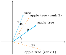
Figure 1: Corrected evaluation: the original representation $\mathbf{\tilde{p}}$ of the compound apple tree is the vector of reference; both original ($\mathbf{v}$) and composed ($\mathbf{p_{1}},\mathbf{p_{2}}$) representations are compared to $\mathbf{\tilde{p}}$ in terms of cosine similarity.

The same procedure is then performed for $\mathbf{p_{2}}$. $\mathbf{p_{2}}$ is compared to the original vectors $\mathbf{\tilde{p}}$ and $\mathbf{v}$ and assigned the rank 1, because $\mathbf{\tilde{p}}$, the original vector for apple tree, is its nearest neighbor.

Herein lies the problem: although $\mathbf{p_{1}}$ is closer to the original representation $\mathbf{\tilde{p}}$ than $\mathbf{p_{2}}$, $\mathbf{p_{1}}$’s rank is worse. This is because the vector of reference is the composed representation, which changes from one composition function to the other. Baroni and Zamparelli (2010)’s formulation of the rank assignment procedure can lead to situations where composed representations rank better even as the distance between the composed and the original vector increases, as illustrated in Fig. 1.

We propose a simple fix for this issue: we compute all the cosine similarities with respect to $\mathbf{\tilde{p}}$, the original representation of each compound or phrase. Having a fixed reference point makes it possible to correctly assess and compare the performance of different composition models. In the new formulation $\mathbf{p_{1}}$ is correctly judged to be the better composed representation, assigned rank 1, whereas $\mathbf{p_{2}}$ is assigned rank 2.

Composition models are evaluated on the test split of each dataset. First, the rank of each composed representation is determined using the procedure described above. Then the ranks of all the test set entries are sorted. We report the first (Q₁), second (Q₂) and third (Q₃) quartile, where Q₂ is the median of the sorted rank list, Q₁ is the median of the first half and Q₃ is the median of the second half of the list. We report two additional performance metrics: the average cosine distance (cos-d) between the composed and the original representations of each test set entry and the percentage of test compounds with rank $\leq$5. Typically, a composed representation can have close neighbors that are different but semantically similar to the composed phrase. A rank $\leq$5 indicates a well-build representation, compatible with the neighborhood of the original phrase.

Another particularity of our evaluation is that the ranks are computed against the full vocabulary of each embedding set. This is in contrast to previous evaluations Baroni and Zamparelli (2010); Dima (2015) where the rank was computed against a restricted dictionary containing only the words and phrases in the dataset. A restricted dictionary makes the evaluation easier since many similar words are excluded. In our case similar words from the entire original vector space can become foils for the composition model, even if they are not part of the dataset. For example the English compounds dataset has a restricted vocabulary of 25,807 words, whereas the full vocabulary contains 270,941 words.

5 Results

Section 5.1 reports on the performance of the different weighting variants proposed for the TransWeight model on the most challenging of the nine datasets, the German compounds dataset. TransWeight with the best weighting is then compared to existing composition models in Section 5.2.

5.1 Performance of different weighting variants

Table 3 compares the performance of the four weighting variants introduced in Section 3.2.

TransWeight-feat, which sums the transformed representations and then weights each component of the summed representation, has the weakest performance, with only 50.82% of the test compounds receiving a rank that is lower than 5.

A better performance – 52.90% – is obtained by applying the same weighting for each column of the transformations matrix $\mathbf{H}$. The results of TransWeight-trans are interesting in two respects: first, it outperforms the feature variation, TransWeight-feat, despite training a smaller number of parameters (300 vs. 400 in our setup). Second, it performs on par with the TransWeight-mat variation, although the latter has a larger number of parameters (20,200 in our setup). This suggests that an effective combination method needs to take into account full transformations, i.e. entire rows of $\mathbf{H}$ and combine them in a systematic way.

TransWeight builds on this insight by making each element of the final composed representation $\mathbf{p}$ dependent on each component of the transformed representation $\mathbf{H}$. The result is a noteworthy increase in the quality of the predictions, with $\sim$12% more of the test representations having a rank $\leq$5.

Although this weighting does use significantly more parameters than the previous weightings (4,000,200 parameters), the number of parameters is relative to the number of transformations $t$ and does not grow with the size of the vocabulary. As the results in the next subsection show, a relatively small number of transformations is sufficient even for larger training vocabularies.

Model	W param	Cos-d	Q1	Q2	Q3	$\leq$5
TransWeight-feat	$n+n$	0.344	2	5	28	50.82%
TransWeight-trans	$t+n$	0.338	2	5	24	52.90%
TransWeight-mat	$tn+n$	0.338	2	5	25	53.24%
TransWeight	$tn^{2}+n$	0.310	1	3	11	65.21%

Table 3: Different weighting variations evaluated on the compounds dataset (32,246 nominal compounds). All variations use $t=100$ transformations, word representations with $n=200$ dimensions and the dropout rate that was observed to work best on the dev dataset (see Appendix B for details). Results on the 6442 compounds in the test set of the German compounds dataset.

5.2 Comparison to existing composition models

	Nominal Compounds					Adjective-Noun Phrases					Adverb-Adjective Phrases
Model	Cos-d	Q1	Q2	Q3	$\leq$5	Cos-d	Q1	Q2	Q3	$\leq$5	Cos-d	Q1	Q2	Q3	$\leq$5
	English
Addition	0.408	2	7	38	46.14%	0.431	2	7	32	44.25%	0.447	2	5	15	53.01%
SAddition	0.408	2	7	38	46.14%	0.421	2	5	26	50.95%	0.420	1	3	8	67.76%
VAddition	0.403	2	6	33	47.95%	0.415	2	5	22	53.30%	0.410	1	2	6	71.94%
Matrix	0.354	1	2	9	67.37%	0.365	1	2	6	74.38%	0.343	1	1	2	91.17%
WMask+	0.344	1	2	7	71.53%	0.342	1	1	3	82.67%	0.335	1	1	2	93.27%
BiLinear	0.335	1	2	6	73.63%	0.332	1	1	3	85.32%	0.331	1	1	1	93.59%
FullLex+	0.338	1	2	7	72.82%	0.309	1	1	2	90.74%	0.327	1	1	1	94.28%
TransWeight	0.323	1	1	4.5	77.31%	0.307	1	1	2	91.39%	0.311	1	1	1	95.78%
	German
Addition	0.439	9	48	363	17.49%	0.428	4	13	71	32.95%	0.500	4	19	215.5	29.87%
SAddition	0.438	9	46	347	18.02%	0.414	2	8	53	42.80%	0.473	2	7	99.5	45.44%
VAddition	0.430	8	39	273	19.02%	0.408	2	7	43	45.14%	0.461	2	5	52	51.12%
Matrix	0.363	3	8	45	41.88%	0.355	1	2	8	68.67%	0.398	1	1	5	76.41%
WMask+	0.340	2	5	25	52.05%	0.332	1	2	5	77.68%	0.387	1	1	3	80.94%
BiLinear	0.339	2	5	26	53.46%	0.322	1	1	3	81.84%	0.383	1	1	3	83.02%
FullLex+	0.329	2	4	20	56.83%	0.306	1	1	2	86.29%	0.383	1	1	3	83.13%
TransWeight	0.310	1	3	11	65.21%	0.297	1	1	2	89.28%	0.367	1	1	2	87.17%
	Dutch
Addition	0.477	5	27	223.5	27.74%	0.476	3	13	87	35.63%	0.532	3	9	75	38.04%
SAddition	0.477	5	27	221	27.71%	0.462	2	7	65	44.95%	0.503	2	4	34	55.57%
VAddition	0.470	4	22	177	29.09%	0.454	2	6	47	48.13%	0.486	1	3	14	63.18%
Matrix	0.411	2	5	26	52.19%	0.394	1	2	6	74.92%	0.445	1	1	4	78.39%
WMask+	0.378	1	3	15	60.14%	0.378	1	1	4	80.78%	0.429	1	1	2	83.02%
BiLinear	0.375	1	3	19	59.23%	0.375	1	1	3	81.50%	0.426	1	1	2	83.57%
FullLex+	0.388	1	3	14	60.84%	0.362	1	1	2	85.24%	0.433	1	1	3	82.36%
TransWeight	0.376	1	2	11	66.61%	0.349	1	1	2	88.55%	0.423	1	1	2	84.01%

Table 4: Results for English, German and Dutch on the composition of nominal compounds, adjective-noun phrases and adverb-adjective phrases.

The composition models discussed so far were evaluated on the nine datasets introduced in Section 4.1. The results using the corrected rank evaluation procedure described in Section 4.4 are presented in Table 4.

TransWeight, the composition model proposed in this paper, delivers consistent results, being the best performing model across all languages and phrase types. The difference in performance to the runner-up model, FullLex+, translates into more of the test phrases being close to the original representations, i.e. achieving a rank $\leq 5$. This difference ranges from 8% of the test phrases in the German compounds dataset to less than 1% for English adjective-noun phrases. However, it is important to note the substantial difference in the number of parameters used by the two models: all TransWeight models use 100 transformations and have, therefore, a constant number of 12,020,200 parameters. In contrast the number of parameters used by FullLex+ increases with the size of the training vocabulary, reaching 739,320,200 parameters in the case of the English adjective-noun dataset.

The most difficult task for all the composition models in any of the three languages is compound composition. We believe this difficulty can be mainly attributed to the complexity introduced by the position. For example in adjective-noun composition, the adjective always takes the first position, and the noun the second. However, in compounds the same noun can occur in both positions throughout different training examples. Consider for example the compounds boat house and house boat. In boat house – a house to store boats – the meaning of house is shifted towards shelter for an inanimate object, whereas house boat selects from house aspects related to human beings and their daily lives happening on the boat. These position-related differences can make it more challenging to create composed representations.

Another aspect that makes the adverb-adjective and adjective-noun datasets easier is the high dataset frequency of some of the adverbs/adjectives. For example, in the English adjective-noun dataset a small subset of 52 adjectives like new, good, small, public, etc. are extremely frequent, occurring more than 500 times in the training portion of the adjective-noun sample dataset. Because the adjective is always the first element of the composition, the phrases that include these frequent adjectives amount to around 24.8% of the test dataset. Frequent constituents are more likely to be modeled correctly by composition – thus leading to better results.

The additive models (Addition, SAddition, VAddition) are the least competitive models in our evaluation, on all datasets. The results strongly argue for the point that additive models are too limited for composition. An adequate composed representation cannot be obtained simply as an (weighted) average of the input components.

The Matrix model clearly outperforms the additive models. However, its results are modest in comparison to models like WMask+, BiLinear, FullLex+ and TransWeight. This is to be expected: having a single affine transformation limits the model’s capacity to adapt to all the possible input vectors $\mathbf{u}$ and $\mathbf{v}$. Because of its small number of parameters, the Matrix model can only capture the general trends in the data.

More interaction between $\mathbf{u}$ and $\mathbf{v}$ is promoted by the BiLinear model through the $d$ bilinear forms in the tensor $\mathbf{E}\in\mathbb{R}^{n\times d\times n}$. This capacity to absorb more information from the training data translates into better results — the BiLinear model outperforms the Matrix model on all datasets.

In evaluating FullLex we tried to mitigate its treatment of unknown words. Instead of using unknown matrices to model composition of phrases not in the training data, we take a nearest neighbor approach to composition. Take for example the phrase sky-blue dress, where sky-blue does not occur in train. Our implementation, FullLex+, looks for the nearest neighbor of sky-blue that appears in train, blue and uses the matrix associated with it for building the composed representation. The same approach is also used for the WMask model, which is referred to as WMask+.

The use of datasets with a range of different sizes revealed that datasets with a smaller number of phrases per unique word can be successfully modelled using only transformation vectors. However, datasets with a larger number of phrases per word require the use of transformation matrices in order to generalize. For example, the Dutch compounds dataset has 5,317 unique words and 17,773 phrases, resulting in 3.3 phrases per word. On this dataset WMask+ fares only slightly worse than FullLex+ (0.70%), an indication that FullLex+ suffers from data sparsity in such scenarios and cannot produce good results without an adequate amount of training data. By contrast, the gap between the two models increases considerably on datasets with more phrases per word — e.g. FullLex+ outperforms WMask+ with 8.07% on the English adjective-noun phrase dataset, which has 11.6 phrases per word.

We compared FullLex+ and TransWeight in terms of their ability to model phrases where at least one of the constituents is not part of the training data. For example 16.2% of the test portion of the English compounds dataset, 563 compounds, have at least one constituent that is not seen during training. We evaluated FullLex+ and TransWeight on this subset of data: 59.15% of the representations composed using FullLex+ obtain a rank $\leq 5$. When using TransWeight, a rank $\leq 5$ is obtained for 67.50% of the representations. The difference between the two results is an indicator of the superior generalization capabilities of TransWeight.

TransWeight is the top performing composition model on small and large datasets alike. This shows that treating similar words similarly — and not each word as a semantic island — has a two-fold benefit: (i) it leads to good generalization capabilities when the training data is scarce and (ii) gives the model the possibility to accommodate a large number of training examples without increasing the number of parameters.

5.3 Understanding TransWeight

The results in Section 5.2 have shown that the transformations-based generalization strategy employed by TransWeight works well across different languages and phrase types. However, understanding what the transformations encode requires taking a step back and contemplating again the architecture of the model.

Each transformation used by the model can be seen as a separate application of an affine transformation of the concatenated input vectors $[\mathbf{u};\mathbf{v}]\in\mathbb{R}^{2n}$ – essentially, one Matrix model – resulting in a vector in $\mathbb{R}^{n}$. 100 transformations provide 100 ways of combining the same pair of input vectors.

Two competing hypotheses can be put forth about the way each transformation contributes to the final representation. The specialization hypothesis assumes that each transformation specializes on particular input types e.g. bigrams made of color adjectives and artifact-like nouns like black car. In contrast, the distribution hypothesis assumes that the parameters responsible for particular bigrams are distributed across the transformations space instead of being confined to any single transformation.

If the specialization hypothesis holds, removing the transformations that are tailored to a particular input type will drastically reduce the performance on instances of that input type. In order to test this hypothesis, we evaluated TransWeight while randomly dropping full transformations at dropout rates between 0% and 90% during prediction. This procedure also removes between 0% and 90% of the specialized transformations — assuming that they exist.

The performance of the model with transformation dropout is hard to interpret in isolation, since it is to be expected that the performance of a model decreases as side-effect of removing parameters. Thus, any loss of performance can be attributed to the removal of specific transformations or to the reduction of the number of parameters in general. In order to make the results interpretable, we have created a reference model that drops individual parameters of the transformed representations, rather than dropping full transformations. The reference model removes the same number of parameters as the model with transformation dropout, but keeps specific transformations partially intact. This allows us to verify whether the loss of performance of dropping out transformations is larger than the expected loss of removing (any) parameters. If this is indeed the case, removing certain transformations is more harmful than removing random parameters and the specialization hypothesis should be accepted. On the other hand, if there is no tangible difference between the two models, then the specialization hypothesis should be rejected in favor of the distribution hypothesis.

The results of this experiment on the English adjective-noun set are shown in Figure 2, which plots the percentage of ranks $\leq 5$ against the dropout rate. Since there is virtually no difference in losses between the model that uses transformation dropout and the reference model, we reject the specialization hypothesis. However, rejecting the specialization hypothesis does not exclude the possibility that semantic properties of specific classes of words are captured by parameters distributed across the transformations.

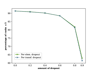
Figure 2: The percentage of ranks $\leq 5$ of the model that drops transformations randomly and the refence model that drops individual parameters of transformed representations randomly.

6 Conclusion

In this paper we have introduced TransWeight, a new composition model which uses a set of weighted transformations, as a middle ground between a fully lexicalized model and models based on a single transformation. TransWeight outperforms all other models in our experiments.

In this work, we have trained TransWeight for specific phrase types. In the future, we would like to investigate whether a single TransWeight model can be used to perform composition of different phrase types, possibly while integrating information about the structure of the phrases and their context as in Hermann and Blunsom (2013); Yu et al. (2014); Yu and Dredze (2015).

Another extension that we are interested in is to use TransWeight to compose more than two words. We plan to follow the lead of Socher et al. (2012) here, which uses the FullLex composition function in a recursive neural network to compose an arbitrary number of words. Similarly, we could use TransWeight in a recursive neural network in order to compose more than two words.

In our experiments, 100 transformations yielded optimal results for all phrase sets. However, further investigation is needed to determine if this number is optimal for any combination of word classes, or whether it is dependent on the word class type (i.e. open or closed), the diversity of the word classes in a dataset, or properties of the embedding space that are inherent to the method used to construct the vector space.

	Nominal Compounds					Adjective-Noun Phrases					Adverb-Adjective Phrases
Model	Cos-d	Q1	Q2	Q3	$\leq$5	Cos-d	Q1	Q2	Q3	$\leq$5	Cos-d	Q1	Q2	Q3	$\leq$5
	English
WMask+	0.344	3	9	43	39.84%	0.342	4	11	41	33.23%	0.335	3	8	33	40.86%
BiLinear	0.335	3	7	33	43.81%	0.332	3	9	33	39.14%	0.331	2	7	25	45.84%
FullLex+	0.338	3	9	41.5	40.53%	0.309	2	6	20	48.41%	0.327	2	7	25	45.45%
TransWeight	0.30	2	7	34	44.44%	0.307	3	9	33	39.36%	0.31	2	6	19	49.05%
	German
WMask+	0.34	3	12	89	37.01%	0.35	5	19	92	25.52%	0.387	8	40	219.5	18.32%
BiLinear	0.334	3	11	97	38.73%	0.34	5	15	74	29.51%	0.383	7	29	163	21.83%
FullLex+	0.328	3	10	72	39.89%	0.343	4	12	58	32.49%	0.383	7	35	189	20.55%
TransWeight	0.31	2	10	76	40.10%	0.324	4	14	68	30.24%	0.367	6	24	130	23.21%
	Dutch
WMask+	0.393	7	39	307	21.09%	0.378	6	20	132	24.87%	0.429	9	44	315	17.42%
BiLinear	0.396	6	34	284	24.37%	0.375	5	19	140	27.40%	0.426	8	34	239	19.18%
FullLex+	0.388	6	37	313.5	22.93%	0.362	4	13	80	31.57%	0.433	10	50	381	16.65%
TransWeight	0.376	5	28	235.5	25.25%	0.349	5	18	16	26.92%	0.423	8	29	238	18.96%

Table 5: Results using the Baroni and Zamparelli (2010) evaluation method for the best performing models for English, German and Dutch on the composition of nominal compounds, adjective-noun phrases and adverb-adjective phrases.

Appendix A Hyperparameters word embeddings

The word embeddings were trained using the skip-gram model with negative sampling Mikolov et al. (2013) from the word2vec package. Arguments: embedding size of 200; symmetric window of size 10; 25 negative samples per positive training instance; and a sample probability threshold of $10^{-4}$. As a default, we use a minimum frequency cut-off of 50. However, for German adverb-adjective phrases and all Dutch phrases we used a cut-off to 30 to be able to extract enough phrases for training and evaluation.

Appendix B Hyperparameters composition models

Dropout Srivastava et al. (2014) rates between 0 and 0.8 in 0.2 increments were tested on the dev set for the four weighting variations presented in Table 3, while keeping constant the number of transformations (100). TransWeight-r performed best with a dropout of 0.4, TransWeight-c and TransWeight-v with 0.6 dropout and TransWeight with 0.8 dropout. For TransWeight the dropout is applied to $\mathbf{H}$, the matrix containing the transformed representations.

References

- Abadi et al. (2015) Martín Abadi, Ashish Agarwal, Paul Barham, Eugene Brevdo, Zhifeng Chen, Craig Citro, Greg S. Corrado, Andy Davis, Jeffrey Dean, Matthieu Devin, Sanjay Ghemawat, Ian Goodfellow, Andrew Harp, Geoffrey Irving, Michael Isard, Yangqing Jia, Rafal Jozefowicz, Lukasz Kaiser, Manjunath Kudlur, Josh Levenberg, Dan Mané, Rajat Monga, Sherry Moore, Derek Murray, Chris Olah, Mike Schuster, Jonathon Shlens, Benoit Steiner, Ilya Sutskever, Kunal Talwar, Paul Tucker, Vincent Vanhoucke, Vijay Vasudevan, Fernanda Viégas, Oriol Vinyals, Pete Warden, Martin Wattenberg, Martin Wicke, Yuan Yu, and Xiaoqiang Zheng. 2015. TensorFlow: Large-Scale Machine Learning on Heterogeneous Systems. Software available from tensorflow.org.
- Baayen et al. (1993) Harald Baayen, Richard Piepenbrock, and Hedderik van Rijn. 1993. The CELEX lexical data base on CD-ROM.