Evidential positive opinion influence measures for Viral Marketing

Abstract

The Viral Marketing is a relatively new form of marketing that exploits social networks to promote a brand, a product, etc. The idea behind it is to find a set of influencers on the network that can trigger a large cascade of propagation and adoptions. In this paper, we will introduce an evidential opinion-based influence maximization model for viral marketing. Besides, our approach tackles three opinions based scenarios for viral marketing in the real world. The first scenario concerns influencers who have a positive opinion about the product. The second scenario deals with influencers who have a positive opinion about the product and produce effects on users who also have a positive opinion. The third scenario involves influence users who have a positive opinion about the product and produce effects on the negative opinion of other users concerning the product in question. Next, we proposed six influence measures, two for each scenario. We also use an influence maximization model that the set of detected influencers for each scenario. Finally, we show the performance of the proposed model with each influence measure through some experiments conducted on a generated dataset and a real world dataset collected from Twitter.

1 Introduction

The unprecedented growth of social networks made the marketers revalue their strategies in viral marketing. Viral marketing exploits existing social networks and sends viral marketing messages related to a company, brand or product by influencing friends who will recommend intentionally or unintentionally the product to other friends and many individuals will probably adopt it. Hotmail rapidly adopted a viral marketing strategy and reported a significant rise of their business from influence propagation in social networks. Hotmail gained 18 million users in 12 months, spending only $50,000 on traditional marketing [18], while Gmail rapidly gained users although referrals are the only way to sign up.

The phenomenon of influence propagation through social networks has been attracting a great body of research works [19, 11, 2, 25]. However, existing influence maximization approaches assume that all network users and influencers have a positive opinion and the works [33, 5] that consider the user’s positive opinion assume the availability of positive influence probabilities. Whereas, a key function of social networks is sharing, by enabling users to express their opinions about a product or trend of news by means of posts, shared posts, likes/dislikes, or comments on friends’ posts. Such opinions are propagated to other users and might exert an either positive or negative influence on them. For example, if some friends have shown any positive (or negative) comments against a product or news, one will have a similar feeling regardless of their own opinion. Then, the influencer opinion is beneficial for the product if it is positive. However, such an opinion is harmful if it is negative. In fact, according to the social psychology literature [29, 3] the information negativity (negative events, ideas, news, etc.) is always stronger than positivity (positive events, ideas, news, etc.). Consequently, the consideration of the user’s opinion in the influence maximization process is crucial for a given marketing campaign.

The influence maximization (IM) in an online social network (OSN) presents two main challenges: the first challenge is about data imprecision and uncertainty. In fact, social interactions are not always precise and certain. Besides, the OSN API (Application Programming Interface) allows only a limited access to their data which generates more imprecision and uncertainty for the social network analysis fields. Then, if we ignore this imperfection of the data, we may be confronted with erroneous analysis results. The second challenge is about the diversity of influence markers and parameters, e.g. the opinion, the user’s activity, the position in the network, etc. Indeed, it is important to combine all of them to obtain a global influence measure that considers all these parameters, the data imperfection and the conflict that may exist between influence markers. Consequently, it is necessary to resolve these challenges in order to obtain better influence maximization results. For these purposes, we propose the theory of belief functions [7, 27] as a solution. In fact, it was widely applied in many similar situations and it was efficient. Furthermore, this theory was used for analyzing social networks [30, 9, 16, 17, 14, 15, 13].

In this paper, we consider the user’s opinion about the product and we contribute with three opinion-based scenarios of viral marketing. To the best of our knowledge, this is the first work that refines the influencers detection process to be up to the expectations of marketers. In fact, we introduce technical solutions that fit more with purposes of their campaigns. In the first scenario, we investigate influencers who have a positive opinion about the product. The second scenario looks for influencers who have a positive opinion about the product and exert more influence on users with a positive opinion. Finally, the third scenario searches to detect influence users who have a positive opinion about the product and exert more influence on influence users having a negative opinion about the product. For each scenario, we define two evidential influence measures. We use the theory of belief functions to estimate the influence considering data imperfection.

To the best of our knowledge, the work conducted in this paper is the first to achieve the following contributions: 1) we consider the real user’s opinion that is estimated from the posted messages, 2) we introduce three opinion-based scenarios of viral marketing which gives flexible solutions that go with marketers expectations, 3) we propose two evidential opinion-based influence measures for each scenario, 4) we use the theory of belief functions to remedy the data imperfection problems, to fuse influence markers and user opinion efficiently, 5) we maximize the influence in an OSN using the proposed measures, 6) we conduct many experiments on generated data and real-world data collected from Twitter to show the performance of the proposed measures with the used influence maximization model.

This paper is organized as follows: Section 2 reviews some relevant existing works, Section 3 deals with backgrounds of the theory of belief functions that are used in this paper. A few lines later, Section 4 focuses our attention on the introduction of the proposed three opinion-based scenarios of viral marketing. A set of experiments is presented and discussed in Section 5.

2 Related work

The influence maximization (IM) is a very common problem that has been widely studied since its introduction [8, 19, 22]. It searches to select a set of $k$ users in the social network that could adopt the product and trigger a large cascade of adoptions and propagation through the “word of mouth” effect. The selected users are commonly called influencers. In the literature, we find many solutions for the IM problem. In this section, we present an overview of the state of the art.

2.1 Influence maximization: an overview

The influence maximization (IM) is the problem of finding a set $S$ of $k$ influence users that can trigger a large cascade of propagation and adoption. The set $S$ is called seed set. A very common application of this problem is the viral marketing [22]. Indeed, in a viral marketing campaign, the marketer wishes to propagate propaganda and to make it go viral. Then, he needs a set of influencers to be the triggers of the campaign. Those influencers will start the propagation process. Kempe et al. [19] were the first to define the problem of detecting influencers as a maximization problem. Besides, they proved the NP-Hardness of this problem. Given a social network $G=\left(V,E\right)$, where $V$ is the set of nodes and $E$ is the set of links, they defined $\sigma_{M}\left(S\right)$ as the expected number of influenced nodes in the network. Next, Kempe et al. [19] showed that $\sigma_{M}\left(S\right)$ is monotone, i.e. $\sigma_{M}\left(S\right)\leq\sigma_{M}\left(T\right)$ whenever $S\subseteq T\subseteq V$, and sub-modular, i.e. $\sigma_{M}\left(S\cup\left\{x\right\}\right)-\sigma_{M}\left(S\right)\geq\sigma_{M}\left(T\cup\left\{x\right\}\right)-\sigma_{M}\left(T\right)$ whenever $S\subseteq T\subseteq V$ and $x\in V$. In the influence maximization step, i.e. maximizing $\sigma_{M}\left(S\right)$, the authors proposed the greedy algorithm with the Monte Carlo simulation.

To calculate $\sigma_{M}\left(S\right)$, [19] used two existing propagation models: the Linear Threshold Model (LTM) [12] and the Independent Cascade Model (ICM) [10]. A node $v$ is active if it receives the propagated information and accepts it, elsewhere, it is inactive. An inactive vertex can change its status to active. The ICM model considers that each active vertex $u$ has only one chance to activate its neighbors. Indeed, when a given node $u$ becomes active at $t$, it will try to activate its inactive neighbor $v$ at $t+1$ with a success probability $p\left(u,v\right)$ (parameter of the system). The Weighted Cascade (WC) is a special case of ICM where

$$p\left(u,v\right)=\frac{1}{D_{u}}$$ (1)

such that $D_{u}$ is the degree of the node $u$. The LTM model has another activation condition based on a node threshold $\theta_{u}$. It associates a weight $\omega\left(u,v\right)$ to each link $\left(u,v\right)$ and a threshold $\theta_{u}$ to each node $u$. A given inactive node $u$ changes its status to active if the following condition is true:

$$\sum_{v}\omega\left(u,v\right)\geq\theta_{u}$$ (2)

where $\theta_{u}\in\left[0,1\right]$ is a random uniform variable and it is defined as the tendency of a given node $u$ to adopt the information when its neighbors do.

The work of [31, 23] studied the influence propagation using the Page Rank algorithm. In fact, they studied the connection between the social influence and Page Rank and they found that Page Rank information can be helpful to find influencers. Xiang et al. [31] introduced a linear social influence model that approximates ICM. Next, they showed that the Page Rank algorithm is a special case of their algorithm. The work of Liu et al. [23] is an extension of [31] in which they consider nodes’ prior knowledge to better identify influencers. We find also, the work of [32] that introduced a marketing campaign recommender system udapted for Business to Business (B2B). Their work is interesting as it considers “the temporal behavior patterns in the B2B buying processes” [32]. We notice that these solutions do not consider the user opinion which implicates a hidden assumption that considers all influencers as positive.

Another interesting influence maximization model was introduced by Goyal et al. [11]. It is a data-based model called credit distribution (CD). It takes two main inputs which are the network structure and propagation log. It uses these inputs to estimate the influence. In fact, the influence spread function is defined as the total influence credit given to a set of users $S$ from the whole network. The idea behind this algorithm is when an action $a$ propagates from a user $v$ to a user $u$, a direct influence credit $\gamma_{v,u}\left(a\right)$ is given to $v$. Furthermore, a credit amount is given to the predecessors of $v$. The credit distribution algorithm starts by scanning the action log $L$ (the set of tuples $\left(User,\,Action,\,Time\right)$ where $\left(v,a,t\right)\in L$ when $v$ performed the action $a$ at time $t$) and estimates the total influence credit given to $v$ for influencing $u$ on the action $a$, $\Gamma_{v,u}\left(a\right)$. Initially, we have $S=\emptyset$. Next, CD runs up the CELF algorithm to detect the vertex having the maximum marginal gain and so on until having $k$ nodes in $S$. More details can be found in [11].

As the work of [11], we consider past propagation for influence maximization. However, the proposed approach differs from their solution. In fact, we consider the user’s opinion about the product and the opinions of the influencer neighbors.

2.2 Opinion-based influence maximization

In this section, we are mainly interested in works that incorporate the user’s opinion in the influence maximization process which is a relatively new idea. In fact, the user’s opinion is a critical factor in marketing and social science. In the social psychology literature, the concept of positive-negative opinion asymmetry was largely studied [29, 3]. These works agreed on the fact that negativity (negative events, ideas, news, etc.) is always stronger than positivity (positive events, ideas, news, etc.). This fact was, also, shown in marketing science like the work of Cheung and lee [6] that studied the impact of the negative electronic word of mouth (eWoM) on online shops and they found that “negative eWoM has a significantly larger impact on consumer trust and intention to the online shop”. These works prove the importance of the opinion in the influence maximization process and especially the importance of selected seed’s opinion.

Chen et al. [5] extended the influence propagation model of Kempe et al. [19] and incorporated the negative opinions and their propagation into the influence maximization process. On an interesting work, Zhang et al. [33] proposed the Opinion-based Cascading (OC) model that takes positive opinions of users into consideration. They used the OC model to maximize the positive influence by considering the user’s opinion and the change of the opinion. They showed that the objective function of the OC model is no longer submodular. Besides, they proved the NP-Hardness of their model. Then, they proposed an approximation of the maximization results in a polynomial time. In a first step, OC ignores all users that have a small potential marginal gain that is defined as:

$$PMG\left(v\right) = Op\left(v\right)+\sum_{u\in N_{out}^{a}\left(v\right)}\left(Op\left(u\right)+Op\left(v\right).w\left(v,u\right)\right)$$ (3)

$$+ \sum_{u\in N_{out}^{ia}\left(v\right)}\frac{w\left(v,u\right)}{\theta_{u}}\left(Op\left(u\right)+Op\left(v\right).w\left(v,u\right)\right)$$

where $Op\left(v\right)$ defines the opinion indicator of $v$ such that $Op\left(v\right)=0$ means that $v$ has a neutral opinion, $Op\left(v\right)>0$ indicates that the opinion is positive, $Op\left(v\right)<0$ the opinion of $v$ is negative. The sets $N_{out}^{a}\left(v\right)$ and $N_{out}^{ia}\left(v\right)$ are respectively, the sets of $v$’s active and inactive out-neighbors, i.e. the set of destinations of directed links having $v$ as source. The parameter $\theta_{u}$ defines the activation probability of $u$. Finally, $w\left(v,u\right)$ is the weight associated to the edge $\left(v,u\right)$. In the next step, OC iterates until getting $k$ seed nodes. In each iteration, the algorithm updates the activation status according to the condition $\sum_{u\in N_{in}^{a}\left(v\right)}w\left(u,v\right)\geq\theta_{v}$ where $N_{in}^{a}\left(v\right)$ is the set of active in-neighbors of $v$. Also, it updates the opinion value of each user according to his previously activated neighbors as:

$$Op\left(v\right)=Op\left(v\right)+\sum_{u\in N_{in}^{a}\left(v\right)}\left(Op\left(u\right).w\left(u,v\right)\right)$$ (4)

Then, OC chooses the user that still in the top of the potential list. Li et al. [21] considered not only the friendship relations but also foe relations in the influence maximization problem. They used a signed network, i.e. positive relations $\left(+\right)$ to model friendship or trust and negative relations $\left(-\right)$ to model foes or distrust.

These recent works assumed that positive and negative influence probabilities are known and given to the influence maximization algorithm as input. This is obviously not the case in real-world propagation. Indeed, some preprocessing is needed to close the gap between the model and the real data [11]. Furthermore, we tested the opinion-based cascading model on real world data and with estimated opinion values. According to these experiments, the opinion-based cascading model detected several inactive and isolated users, even, the mean positive opinion of the selected influencers is less than 50% which is not a satisfying result. The reader can refer to Section 5 for more details. These tests confirmed the need for efficient solutions that deals with these drawbacks.

2.3 Influence and evidence theory

In the literature, there are some recent works that use the theory of belief functions to model the uncertainty while measuring user influence in online social networks. In this section, we will present a brief review of the works that we find close to our work.

Authors in [30] presented an evidential centrality (EVC) measure. EVC is the result of the combination of two BBAs distributions on the frame $\left\{high,\,low\right\}$. The first BBA is used to measure the degree centrality and the second one is used to measure the strength centrality of the node. The work of [9] proposed a centrality measure with a same spirit as EVC. In fact, they modified the EVC measure according to the actual degree of the node instead of following the uniform distribution, also, they extended the semi-local centrality measure [4] to be used with weighted networks. Their centrality measure is the result of the combination of the modified EVC and the modified semi-local centrality measure. The work of [9] is similar to the work of [30] in that, they used the same frame of discernment, their approaches are structure based and they choose the influential nodes to be top-1 ranked nodes according to the proposed centrality measure.

Our work is like the work of [30] and [9] in that we used the same BBA estimation mechanism of the influence BBA. More details about the influence estimation process we use can be found in [15]. Nevertheless, our work is different from their work in that we consider the user’s opinion and we maximized the influence. In fact, the importance of the opinion parameter in the viral marketing campaign encouraged us to consider it in the influence maximization process.

3 Background

In this section, we will introduce some concepts of the theory of belief functions that are used in this paper. This theory is also called Dempster-Shafer theory or evidence theory. Dempster [7] was the first to introduce it through what he called Upper and Lower probabilities. Later, Shafer published his book "A mathematical theory of evidence" [27] in which he defined the basics of the evidence theory. This theory is recommended to process the imprecise and uncertain data. Furthermore, it allows to achieve more precise, reliable and coherent information.

Let $\Omega=\left\{d_{1},d_{2},...,d_{n}\right\}$ be a frame of discernment. The basic belief assignment (BBA), $m^{\Omega}$, is a function that defines the belief on $\Omega$, it is defined as:

$$2^{\Omega} \rightarrow \left[0,1\right]$$

$$A \mapsto m^{\Omega}\left(A\right)$$ (5)

where $2^{\Omega}=\left\{\emptyset,\left\{d_{1}\right\},\left\{d_{2}\right\},\left\{d_{1},d_{2}\right\},...,\left\{d_{1},d_{2},...,d_{n}\right\}\right\}$ is the set of all subsets of $\Omega$ called power set. The mass $m^{\Omega}\left(A\right)$ is the value assigned to the subset $A\subseteq\Omega$ and it must respect:

$$\sum_{A\subseteq\Omega}m^{\Omega}\left(A\right)=1$$ (6)

In the case where we have $m^{\Omega}(A)>0$, $A$ is called focal element of $m^{\Omega}$. A simple mass function or simple BBA has at most two focal elements among them $\Omega$. Let $\alpha\in\left[0,1\right]$, the simple BBA $m^{\Omega}$ is defined as:

$$\begin{cases}m^{\Omega}\left(A\right)&=1-\alpha,\,A\subseteq\Omega\\ m^{\Omega}\left(\Omega\right)&=\alpha\end{cases}$$ (7)

Example.

Let’s consider the well-known example of the murder of Mr. Jones introduced by [28]. Big Boss has a team of assassins composed of three members who are Peter, Paul and Mary. We need to define a frame of discernment that contains all possible assassins: $\Omega$ is formed by: Peter (Pe), Paul (Pa) and Mary (Ma), $\Omega=\left\{Pe,\,Pa,\,Ma\right\}$, and its corresponding power set is:

$$2^{\Omega}=\left\{\emptyset,\left\{Pe\right\},\left\{Pa\right\},\left\{Pe,Pa\right\},\left\{Ma\right\},\left\{Pe,Ma\right\},\left\{Pa,Ma\right\},\left\{Pe,Pa,Ma\right\}\right\}$$ (8)

Big Boss selected a killer from his team using a dice, if he obtains an even number, then the killer is a female, else, the killer is a male. Let’s help the Judge to find the murder. We know that Mr. Jones was murdered and the sex of the murder was selected through a dice. However, there is no information about the choice between Peter and Paul in the case of an odd number.

Knowing this information, we can define the following BBA on $\Omega$:
$m_{1}^{\Omega}\left(\left\{Pe,Pa\right\}\right)=0.5$ and $m_{1}^{\Omega}\left(\left\{Ma\right\}\right)=0.5$. $\square$

The theory of belief functions presents many combination rules that are used to fuse pieces of information. The first combination rule was introduced by Dempster [7] and it is called Dempster’s rule of combination. It fuses two distinct mass distributions into a normalized one, i.e. a BBA $m^{\Omega}$ is said to be normal if $m^{\Omega}\left(\emptyset\right)=0$. Let $m_{1}^{\Omega}$ and $m_{2}^{\Omega}$ be two mass distributions defined on $\Omega$, Dempster’s rule is defined as:

$$m_{1\oplus 2}^{\Omega}\left(A\right)=\begin{cases}\frac{\sum_{B\cap C=A}m_{1}^{\Omega}\left(B\right)m_{2}^{\Omega}\left(C\right)}{1-\sum_{B\cap C=\emptyset}m_{1}^{\Omega}\left(B\right)m_{2}^{\Omega}\left(C\right)},&A\subseteq\Omega\setminus\left\{\emptyset\right\}\\ 0&if\,A=\emptyset\end{cases}$$ (9)

Example.

Table (1) is an example of the Dempster’s rule of combination. $\square$

Table 1: Dempster’s rule example

	$m_{1}^{\Omega}$	$m_{2}^{\Omega}$	Dempster’s rule
$\emptyset$	0	0	0
$\left\{Pe\right\}$	0	0	0
$\left\{Pa\right\}$	0	0	0.1765
$\left\{Pe,Pa\right\}$	0.5	0.3	0.4118
$\left\{Ma\right\}$	0.5	0	0.4118
$\left\{Ma,Pe\right\}$	0	0	0
$\left\{Ma,Pa\right\}$	0	0.3	0
$\Omega$	0	0.4	0

4 Proposed opinion-based influence measures

The user’s opinion plays a main role in the viral marketing. In fact, if a user $A$ shares his negative opinion about a product $x$, then all users that will receive $A$ opinion will have, at least, some doubt about $x$ and that in the case in which $A$ is not an influencer for them. In the case where $A$ is an influence user, then his negative opinion will be harmful for the product $x$. This fact encouraged us to propose new influence measures for online social networks that consider the user’s opinion. Besides, we introduce three opinion-based scenarios of viral marketing that will be helpful for the marketer. In fact, this work offers more flexibility to the marketer to build his viral marketing campaign according to his purposes as we explain:

1. First scenario, Positive influencers: in this scenario we look for influencers who have a positive opinion about the product. It is useful for marketers who are looking for positive influencer spreaders. In this case, the marketer may want to avoid influencers that have a negative opinion, and to target only influence users having a positive opinion. A solution for this scenario was published in Jendoubi et al. [14].

2. Second scenario, Positive influencers influencing positive users: the purpose in this scenario is to find positive influencers that exert more influence on users having a positive opinion about the product. It is destined to marketers who are interested in influence users that have a positive opinion about the product and that exert more influence on users having a positive opinion too. In such a case, the marketer may want to boost the probability of success of his viral marketing campaign.

3. Third scenario, Positive influencers influencing negative users: the main goal of this scenario is to detect positive influencers that exert more influence on users having a negative opinion about the product. It is useful for marketers who are looking for influence users that have a positive opinion about the product and that exert more influence on users having a negative opinion. The marketing strategy here may be, for example, to try to gain more customers by changing the opinion of users that have a negative opinion.

The set of positive influencers may include positive influencers influencing positive users and positive influencers influencing negative users. However, the second and the third scenarios have a more specific selection criteria as they have a condition on the neighbor’s opinions of the positive influencer.

In this section, we introduce the opinion polarity estimation process. Next, we present two influence measures for each scenario. Finally, we introduce the influence spread function.

4.1 Opinion polarity estimation

In this paper, we consider the user’s opinion about the product in the maximization process. For this purpose, we need to estimate this opinion. First, we start by estimating the opinion polarity of each message, then, we take the user’s opinion as the mean opinion of his posted messages. We remark that the message may depend on the considered online social network (OSN). For example, it can be a tweet, a retweet or a reply if the OSN is Twitter, it can be a wall post or a comment if the OSN is Facebook, it is a post activity or a comment in GooglePlus. Next, we explain the process we used to estimate the opinion expressed in a given message.

To estimate the opinion polarity of each given message, we used existing tools that are dedicated for this purpose. We followed the following process:

1. We deleted URLs and special characters to simplify the estimation task.

2. The second step is called part of speech tagging its goal is to attribute a label (noun, adjective, verb, adverb) to each word in the message. For such a purpose, we used the java library “Stanford part-of-speech Tagger”. We note that the Stanford tagger allows to train a part-of-speech tagger model using an annotated data corpus. However, it is also possible to use an available part-of-speech tagger model like the “GATE Twitter part-of-speech tagger” that was designed for Twitter and that is able to achieve about 91% of accuracy.

3. We use the SentiWordNet 3.0 [1] dictionary to get the polarity of each word (positive, negative and objective polarity) in the message according to its tag (result of the step 2). The result of this step is a probability distribution defined on $\Theta=\left\{Pos,\,Neg,\,Neut\right\}$ for each word in the message.

4. To compute the global polarity of the tweet we take the mean probability distribution of words probability distributions that compose the message.

Example.

Let us consider the message that says: “Smartphones are good but complicated”. We want to estimate its opinion polarity using the explained process. The given message did not contain a URL or a special character, then the first step is not needed. Table 2 presents the second and the third steps. Finally, the polarity of the given message is:

$$\textrm{Pr}^{\Theta}\left(Pos\right) = 0.152$$ (10)

$$\textrm{Pr}^{\Theta}\left(Neg\right) = 0.125$$ (11)

$$\textrm{Pr}^{\Theta}\left(Neut\right) = 0.723$$ (12)

Table 2: Computing the opinion polarity of a message

	Smartphones	are	good	but	complicated
Part of speech	noun	verb	adj	conjunction	adj
Positive opinion	0	0	0.635	0	0.125
Negative opinion	0	0	0.001	0	0.625
Neutral opinion	1	1	0.364	1	0.25

$\square$

4.2 User opinion-based influence estimation

Given a social network $G=\left(V,E\right)$, where $V$ is the set of nodes and $E$ is the set of links, a frame of discernment expressing opinion $\Theta=\left\{Pos,\,Neg,\,Neut\right\}$, $Pos$ for positive, $Neg$ for negative and $Neut$ for neutral and a probability distribution $\Pr_{u}^{\Theta}$ defined on $\Theta$ that expresses the opinion of the user $u\in V$ about the product. We transform the opinion probability distribution $\Pr_{u}^{\Theta}$ to a mass distribution $m_{u}^{\Theta}$ to consider the uncertainty that may exist in the user’s opinion. We create two simple mass distributions for $\Pr_{u}^{\Theta}\left(Pos\right)$ and $\Pr_{u}^{\Theta}\left(Neg\right)$. In fact, we take $\alpha$, in formula 7 of Section 3, equals to $\Pr_{u}^{\Theta}\left(Pos\right)$ for the first BBA and $\Pr_{u}^{\Theta}\left(Neg\right)$ for the second one. After this step, we obtain two BBAs expressing the user’s positive and negative opinion respectively.

Let us define a frame of discernment expressing influence and passivity $\Omega=\left\{I,P\right\}$, $I$ for influencers and $P$ for passive users, and a basic belief assignment (BBA) function [27], $m_{\left(u,v\right)}^{\Omega}$, defined on $\Omega$ that expresses the influence that exerts the user $u$ on the user $v$. An estimation process for $m_{\left(u,v\right)}^{\Omega}$ was introduced in [15]. The influence measure introduced in [15] does not consider the user’s opinion. In fact, it has an implicit assumption that all network users have a positive opinion about the product which is an unrealistic assumption. In the following, an estimation example of $m_{\left(u,v\right)}^{\Omega}$, this example summarizes the process described in [15].

Example.

Let us consider two users $u$ and $v$ in the network. To estimate the influence that exerts $u$ on $v$, we need to define a set of measurable influence indicators and/or behaviors. For example, the strength of the relationship between $u$ and $v$, the number of times $v$ shares $u$’s messages, etc. In the next step, we estimate a BBA on $\Omega$ for each defined indicator. For this purpose, the estimation process defined in the work of Wei et al. [30] can be used. Let us consider that we have two influence indicators and let $m_{1}^{\Omega}$ and $m_{2}^{\Omega}$ be their respective BBAs: $m_{1}^{\Omega}\left(I\right)=0.5$, $m_{1}^{\Omega}\left(P\right)=0.3$, $m_{1}^{\Omega}\left(\left\{I,P\right\}\right)=0.2$, $m_{2}^{\Omega}\left(I\right)=0.4$, $m_{2}^{\Omega}\left(P\right)=0.5$ and $m_{2}^{\Omega}\left(\left\{I,P\right\}\right)=0.1$. To estimate $m_{\left(u,v\right)}^{\Omega}$ we combine the BBAs of all indicators using the Dempster’s rule (equation 9 of Section 3). Then $m_{\left(u,v\right)}^{\Omega}=m_{1}^{\Omega}\oplus m_{2}^{\Omega}$. $\square$

In the next step, we define two influence measures for each opinion based scenario. Besides, we use the Dempster’s rule of combination for BBAs fusion (equation 9 of Section 3) to obtain $m_{u}^{\Theta}$ that expresses the opinion of $u$.

4.2.1 Positive opinion influencer

The goal in the first scenario is to detect social influencers who have a positive opinion about the product. In fact, we search to avoid negative influencers, because targeting these users may have a harmful effect on the Viral Marketing campaign. For example, the marketer wants to promote his product in an online social network. First, he starts by identifying a set of influencers in the network that maximizes the total influence. Second, he contacts them and tries to convince them to do some advertising for his product. He may give the influencers a free product or a discounting in order to encourage them more to do the advertising. If by chance he falls on some influencers that do not like his product, what would be their reaction in such a case? Then we propose to avoid negative influencers by detecting and targeting positive influencers. As defined above, the mass value $m_{\left(u,v\right)}^{\Omega}\left(I\right)$ measures the influence of $u$ on $v$ but without considering the opinion of $u$ about the product. We define the positive opinion influence of $u$ on $v$ as the positive proportion of $m_{\left(u,v\right)}^{\Omega}\left(I\right)$ and we propose two measures to estimate this proportion as:

$$Inf_{1}^{+}\left(u,v\right) = \textrm{Pr}_{u}^{\Theta}\left(Pos\right).m_{\left(u,v\right)}^{\Omega}\left(I\right)$$ (13)

$$Inf_{2}^{+}\left(u,v\right) = m_{u}^{\Theta}\left(Pos\right).m_{\left(u,v\right)}^{\Omega}\left(I\right)$$ (14)

In formula (13), we weight $m_{\left(u,v\right)}^{\Omega}\left(I\right)$ using $\textrm{Pr}_{u}^{\Theta}\left(Pos\right)$ to estimate the proportion $Inf_{1}^{+}\left(u,v\right)$ [14], while in formula (14) we use $m_{u}^{\Theta}\left(Pos\right)$ to weight $m_{\left(u,v\right)}^{\Omega}\left(I\right)$ to estimate $Inf_{2}^{+}\left(u,v\right)$. Indeed, formula (14) considers the uncertainty of the user’s opinion.

4.2.2 Positive opinion influencers influencing positive users

In the second scenario, we emphasize influence users who have a positive opinion about the product and that are not connected to negative influencers. In the first scenario, we defined two measures that estimate the positive opinion influence of social users. In the second scenario, the goal is to select among positive opinion influencers those that exert more influence on positive users. For this purpose, we defined two measures by weighting $Inf_{1}^{+}\left(u,v\right)$ and $Inf_{2}^{+}\left(u,v\right)$ using $\left(1-\textrm{Pr}_{v}^{\Theta}\left(Neg\right)\right)$ and $\left(1-m_{v}^{\Theta}\left(Neg\right)\right)$ respectively as follows:

$$Inf_{1}^{++}\left(u,v\right) = \textrm{Pr}_{u}^{\Theta}\left(Pos\right).m_{\left(u,v\right)}^{\Omega}\left(I\right).\left(1-\textrm{Pr}_{v}^{\Theta}\left(Neg\right)\right)$$ (15)

$$= Inf_{1}^{+}\left(u,v\right).\left(1-\textrm{Pr}_{v}^{\Theta}\left(Neg\right)\right)$$ (16)

$$Inf_{2}^{++}\left(u,v\right) = m_{u}^{\Theta}\left(Pos\right).m_{\left(u,v\right)}^{\Omega}\left(I\right).\left(1-m_{v}^{\Theta}\left(Neg\right)\right)$$ (17)

$$= Inf_{2}^{+}\left(u,v\right).\left(1-m_{v}^{\Theta}\left(Neg\right)\right)$$ (18)

The proposed measures, $Inf_{1}^{++}$ and $Inf_{2}^{++}$, give more importance to the positive connection. Indeed, the values of $\left(1-\textrm{Pr}_{v}^{\Theta}\left(Neg\right)\right)$ and $\left(1-m_{v}^{\Theta}\left(Neg\right)\right)$ emphasize the positive opinion of $u$’s neighbor. Consequently, multiplying the positive influence that exerts $u$ on $v$ by the positive opinion of $v$ ($\left(1-\textrm{Pr}_{v}^{\Theta}\left(Neg\right)\right)$ and $\left(1-m_{v}^{\Theta}\left(Neg\right)\right)$ respectively) will result an influence measure that considers the positive opinion of the influencer’s neighbor.

4.2.3 Positive opinion influencers influencing negative opinion users

In the third scenario, we give more importance to influence users who have a positive opinion about the product and that exert more influence on negative influencers. Then, we define two influence measures for this scenario by multiplying $Inf_{1}^{+}$ and $Inf_{2}^{+}$ with the non-positive proportion of $v$ opinion using respectively $\left(1-\textrm{Pr}_{v}^{\Theta}\left(Pos\right)\right)$ and $\left(1-m_{v}^{\Theta}\left(Pos\right)\right)$ as:

$$Inf_{1}^{+-}\left(u,v\right) = \textrm{Pr}_{u}^{\Theta}\left(Pos\right).m_{\left(u,v\right)}^{\Omega}\left(I\right).\left(1-\textrm{Pr}_{v}^{\Theta}\left(Pos\right)\right)$$ (19)

$$= Inf_{1}^{+}\left(u,v\right).\left(1-\textrm{Pr}_{v}^{\Theta}\left(Pos\right)\right)$$ (20)

$$Inf_{2}^{+-}\left(u,v\right) = m_{u}^{\Theta}\left(Pos\right).m_{\left(u,v\right)}^{\Omega}\left(I\right).\left(1-m_{v}^{\Theta}\left(Pos\right)\right)$$ (21)

$$= Inf_{2}^{+}\left(u,v\right).\left(1-m_{v}^{\Theta}\left(Pos\right)\right)$$ (22)

The proposed measures, $Inf_{1}^{+-}$ and $Inf_{2}^{+-}$, emphasize negative connections. In fact, the values of $\left(1-\textrm{Pr}_{v}^{\Theta}\left(Pos\right)\right)$ and $\left(1-m_{v}^{\Theta}\left(Pos\right)\right)$ give more importance to neighbors having a negative opinion about the product. Therefore, multiplying the positive influence that exerts $u$ on $v$ by the negative opinion of $v$ ($\left(1-\textrm{Pr}_{v}^{\Theta}\left(Pos\right)\right)$ and $\left(1-m_{v}^{\Theta}\left(Pos\right)\right)$ respectively) will result an influence measure that considers the negative opinion of the influencer’s neighbor.

4.3 Evidential influence maximization

The influence spread function, $\sigma\left(S\right)$, is the function to be maximized in the influence maximization process. It is the global influence of a set of nodes, $S$, on all nodes in the social network. To define $\sigma\left(S\right)$, first, we introduce the amount of influence given to a set of nodes $S\subseteq V$ for influencing a user, $v\in V$, in the network as follows:

$$\Phi\left(S,v\right)=\begin{cases}1&\textrm{if}\,v\in S\\ {\displaystyle\sum_{u\in S}{\displaystyle}\sum_{x\in D_{in}\left(v\right)\cup\left\{v\right\}}Inf\left(u,x\right).Inf\left(x,v\right)}&\textrm{Otherwise}\end{cases}$$ (23)

such that $Inf\left(u,x\right)$ and $Inf\left(x,v\right)$ can be estimated according to the marketing scenario prefixed by the marketer using its corresponding measure as defined in (Section (4.2)), $Inf\left(v,v\right)=1$ and $D_{in}\left(v\right)$ is the set of in-neighbors of $v$, i.e. the set sources of directed links having $v$ as a destination.

Finally, we define the influence spread function $\sigma\left(S\right)$ under the evidential model as the total influence given to $S\subseteq V$ from all nodes in the social network as:

$$\sigma\left(S\right)=\sum_{v\in V}\Phi\left(S,v\right)$$ (24)

In the spirit of the IM problem, as defined by [19], $\sigma\left(S\right)$ is the objective function to be maximized. Let us consider a social network $G=\left(V,E\right)$, where $V$ is the set of nodes and $E$ is the set of links and an objective function $\sigma\left(S\right)$ defined as explained above, then, find the set of nodes $S^{*}$ that maximizes $\sigma\left(S\right)$ as follows:

$$S^{*}=\underset{S}{\textrm{argmax }}\sigma\left(S\right)$$ (25)

To find out $S^{*}$, we used the influence maximization model that was introduced in [15]. This model is the most adapted for characteristic of the opinion based influence measures introduced in this paper. The main goal of the influence maximization model is to select a set of seed nodes $S^{*}$ that maximizes the objective function $\sigma\left(S\right)$. Let $G=\left(V,\,E\right)$ be a directed social network where $V$ is the set of nodes and $E$ is the set of links and $k$ an integer where $k\leq|V|$. We note that the maximization of $\sigma\left(S\right)$ was demonstrated to be a NP-Hard problem [15]. Moreover, the influence spread function was shown to be monotone and sub-modular in [15]. All proof details can be found in [15]. To maximize $\sigma\left(S\right)$, we use the cost effective lazy-forward algorithm (CELF) [20]. It is an extension of the greedy algorithm that is proved to be about 700 times faster than the basic algorithm. Next, we use the second influence maximization model that was introduced in [15].

5 Experiments

This section is mainly dedicated for experiments and results. In fact, we evaluate the proposed influence measures on real world data and generated data. Furthermore, we compare them to existing solutions which are the credit distribution model and the opinion-based cascading model (more details can be found in Section 2). We consider the credit distribution model as base line model. This solution was the first in the literature that considers the past propagation to estimate the influence. The opinion-based cascading model is also considered as a baseline model as it is the first model that considers the user’s opinion.

The real word data is used in this paper to evaluate the proposed opinion-based influence measures. Then, we first study the quality of the selected seeds using each measure. Besides, this dataset is used to study the real opinion of the selected influencers. Next, the generated data is used to study the ability of the influence maximization model to detect the opinion based influencers for each scenario.

5.1 Data gathering and processing

In this section, we present the datasets we used in our experiments. We also detail the process we followed and used tools to obtain our data. Next, we propose two datasets, the first one was collected from Twitter and the second one was randomly generated.

5.1.1 Twitter dataset

In our experiments, we define a Viral Marketing task which is about the promotion of smartphones on Twitter. For this purpose, we crawled Twitter data for the period between September, 8, 2014 and November, 3, 2014. We used the Twitter API through the Twitter4j java library. It is an open-sourced java implementation of the Twitter API, created by Yusuke Yamamoto. Twitter API provides many kinds of data with some limitations, i.e. a limited number of queries per hour or limited response size. In our case, we are interested in collecting tweets written in English, users, who mentions whom and who retweets from whom. Next, we filtered the obtained data by keeping only tweets that talk about smartphones and users having at least one tweet in the data base. In a last step, we used the process explained in the Section 4.1 to estimate the opinion of each user in the dataset about smartphones. This dataset was also used in the experiments of [14, 15]. In this dataset, we have no information about neither the influence users nor the set of users that maximizes the influence. The influence maximization using this dataset allows to evaluate the proposed opinion-based influence measures in a real world case, i.e. the influence users are not known beforehand like in real world cases. Then, we use the proposed solutions to estimate the influence, the passivity of each user and to detect the influencers. Next, we evaluate the quality of the selected influencers and their opinion which allows to evaluate the relevance of the proposed scenarios and measures.

Table 3 presents some statistics about the content of the collected data. Besides, Figure 5.1.1 displays data distributions over users based on the number of followers, mentions, retweets and tweets across our data. The follow relationship is an explicit relation between Twitter user. In fact, when a user $u$ follows another user $v$, $u$ will receive all the activity of $v$. The mention and the retweet are implicit relations in Twitter. Besides, these relations permit the information propagation on the network. Finally, a tweet is 140 characters message.

Table 3: Statistics of the dataset [15]

#User	#Tweet	#Follow	#Retweet	#Mention
36,274	251,329	71,027	9,789	20,300

Data distributions [15]

5.1.2 Generated dataset

The generated data is used in this paper to study the performance of the proposed influence measures. In fact, we generated data in such a way one can know the influencers, the positive influencers, the positive influencers influencing positive users and the positive influencers influencing negative users. Indeed, to the best of our knowledge, there is no available annotated dataset for the influence maximization problem. Besides, annotating the real word dataset is not given. Then comes the solution of the generated dataset to obtain an annotated data that allows the evaluation of the proposed solution. Next, we obtained a useful dataset to study the accuracy of the used influence maximization solutions. Indeed, this dataset is useful to study the adaptability of the used influence maximization model for the problem of the opinion-based influence maximization and for the defined measures. Next, we detail the process we used to obtain this data. The proposed process is parameterizable and allows to study the accuracy variation in terms of each parameter.

Social networks have special characteristics making them different when compared to ordinary graphs. Among these characteristics, we find the small world assumption [26]. For this reason, we selected a random sampling from Twitter dataset (Section 5.1.1). The resulting network contains 1,010 vertices and 6,906 directed links. Next, we defined a set of influence users. These users are chosen according to their number of outlinks. Besides, this number is fixed according to the assumption that the number of influencers is about 10% of the total number of users in the network. Then, we defined an influencer in this dataset to be a user having at least 15 outlinks. As a result, 108 users are selected. In fact, taking a number of outlinks less than 15 will lead to more selected users, and taking a number greater than 15 will lead to a small number of influencers in this experiment. Then, we consider this value the most adapted for the network we have.

In the next step, we defined randomly, the influence of each user in the network by keeping the selected 108 users as top influencers. Then, we assigned an influence value to each link in the network. We fixed “the minimum value of influence” as a parameter of the random process. In a third step, we selected positive influencers among the fixed set of influencers and we assigned to them a positive opinion. The “minimum value of positive opinion” is a parameter to the random process. In a last step, we defined among positive influencers those that influences positive and negative users. For this purpose, we divided the set of positive influencers into two random subsets. The first subset is for positive influencers influencing positive users, then, we set the opinion of the influencers neighbors to positive. The second subset is for positive influencers influencing negative users and we set the opinion of their neighbors to negative. We notice that there are two more parameters of the random process which are the “minimum positive and negative opinion of positive influencers’ neighbors”.

Using the defined random process, we assign to each link in the network three random values which are the influence, the positive opinion and the negative opinion. The random opinions are used to define influencers for each scenario. We note that we consider a user more influencer when his influence value is near 1. Then, we fix the “minimum value of influence” to study the behavior of the maximization model when the influence increases which gives an idea about realistic cases. However, fixing the maximum value of influence is not realistic. Indeed, when the maximum is near 0, then there is no influencer in the network. Besides, when the maximum is near to 1, then the system will consider all the users in the network as influencers.

5.2 Impact of the opinion incorporation

In this section, we perform some experiments to study the impact of the user’s opinion about the product on the detected seeds. The task we propose is about the influence maximization to promote smartphones on Twitter. The main purpose of this task is to find a set of $k$ influencer users that are able to maximize the global positive influence through the network and to promote the adoption of smartphones. We use the dataset collected from Twitter, the reader can refer to Section 5.1.1 for more details. Let us define $Inf\left(u,v\right)=m_{\left(u,v\right)}^{\Omega}\left(I\right)$ to be the evidential influence measure that does not consider the user’s opinion. An estimation process of this measure was introduced in [15]. Furthermore, we use the second evidential model introduced in [15] with the proposed influence measures as follows:

• The evidential influence measure, $Inf$, ($Inf\left(u,v\right)=m_{\left(u,v\right)}^{\Omega}\left(I\right)$), called “Evidential model”. This model and evidential measure were presented in detail in [15].

• The first measure of the first scenario, $Inf_{1}^{+}$, (equation (13)), called “First scenario with probability opinion”.

• The second measure of the first scenario, $Inf_{2}^{+}$, (equation (14)), called “First scenario with belief opinion”.

• The first measure of the second scenario, $Inf_{1}^{++}$, (equation (15)), called “Second scenario with probability opinion”.

• The second measure of the second scenario, $Inf_{2}^{++}$, (equation (17)), called “Second scenario with belief opinion”.

• The first measure of the third scenario, $Inf_{1}^{+-}$, (equation (19)), called “Third scenario with probability opinion”.

• The second measure of the third scenario, $Inf_{2}^{+-}$, (equation (21)), called “Third scenario with belief opinion”.

In the following experiments, we fixed $k$ to $50$ and we compared the proposed solutions to the Credit Distribution model (CD) [11] and to the Opinion-based Cascading (OC) model [33]. We note that we adapted the CD model to Twitter data by defining two actions which are the mention and the retweet. Then, we estimated the credit of each user in the network using these two actions as defined in the algorithm (see Section 2.1). Furthermore, we used the estimated opinion values (used in the proposed measures) to define the function $Op\left(v\right)$ of the OC model (see Section 2.2 for more details about OC). Each of these two models has some common properties with the proposed influence maximization solutions. In fact, the credit distribution influence measure uses past propagation to estimate the influence as the proposed measures, but it does not consider the opinion. Besides, OC considers the user’s opinion in its influence maximization process. However, it does not use past propagation to estimate the influence.

In a first experiment, we compare the number of common selected seeds on Twitter dataset as shown in Table 5.2. Then, we examine the amount of common selected seeds between each two couples of models. Indeed, the number of common selected seeds can be seen as a similarity indicator between influence maximization models. Then, it shows if there are some similarities between the experimented models. Furthermore, this experiment is important as it allows to understand the extent to which the user’s opinion has an impact on the set of selected seeds. We notice that the Opinion-based Cascading model (OC) has no common seeds with any experienced model. Besides, CD model has no more than nine common seeds with “Evidential model” that uses an influence measure on the set $\left\{Inf_{1}^{+},\,Inf_{2}^{+},\,Inf_{1}^{++},\,Inf_{2}^{++}\right\}$. However, CD has only one common seed with “Evidential model” with $\left\{Inf_{1}^{+-},\,Inf_{2}^{+-},\,Inf\right\}$. Furthermore, “Evidential model” has a little number of common seeds with other experienced models. However, we have at least 34 common seeds between any couple of models using any influence measure from the set $\left\{Inf_{1}^{+},\,Inf_{2}^{+},\,Inf_{1}^{++},\,Inf_{2}^{++}\right\}$. Besides, the “third scenario with belief opinion” and “third scenario with probability opinion” have 47 common seeds. We explain these observations by the fact that the used opinion-based influence measures are similar because all of them are based on the evidential influence measure, $Inf$.

Seed sets intersection OC CD Evidential model Third scenario with belief opinion Third scenario with probability opinion Second scenario with belief opinion Second scenario with probability opinion First scenario with belief opinion First scenario with probability opinion First scenario with probability opinion 0 9 9 17 17 40 35 38 50 First scenario with belief opinion 0 7 7 15 15 34 42 50 Second scenario with probability opinion 0 9 9 18 18 40 50 Second scenario with belief opinion 0 8 8 18 18 50 Third scenario with probability opinion 0 1 16 47 50 Third scenario with belief opinion 0 1 13 50 Evidential model 0 1 50 CD 0 50 OC 50

In a second experiment, we compare the mean positive and negative opinions of the selected seeds and their neighbors using each maximization model on Twitter dataset as shown in Table 4. This experiment allows to evaluate each experimented model in terms of the opinion of selected seeds and their neighbors. Indeed, we seek influencers according to their positive opinions and to the opinion of their neighbors, then it is interesting to verify if this condition was satisfied in the selected seed set. In Table 4, “Evidential model” that uses the evidential influence measure, $Inf$, selects influencer spreaders that have a moderate positive and negative opinion, about $0.3$. This fact is expected, because $Inf$ does not consider the user’s opinion. Besides, the CD model chooses influencers that have a small value of positive and negative opinion, about $0.01$, which proves that it is not adaptable for this purpose. In fact, CD does not consider the user’s opinion [14]. However, the OC model selects seeds with about $0.41$ of mean positive opinion which still an unsatisfactory result for a model that considers the user’s opinion about the product.

In another hand, when we consider the user’s opinion, we notice better results in the “mean positive opinion” and “mean negative opinion” of selected seeds. Indeed, models that use an influence measure from the set
$\left\{Inf_{1}^{+},\,Inf_{2}^{+},\,Inf_{1}^{++},\,Inf_{2}^{++}\right\}$, select seeds having at least about $0.82$ of “mean positive opinion” and at most about $0.08$ “mean negative opinion” which is an impressive result compared to the results of existing models (CD and OC). In Table 4, we notice that the best maximization model in terms of mean positive and negative opinion is the “First scenario with belief opinion”. In fact, it gives a maximum value of “mean positive opinion”, which equals to $0.85\pm 0.06$ ($0.95$ confidence interval), and a minimum value of “mean negative opinion”, which equals to $0.06\pm 0.03$. Furthermore, we observe that all results of “Evidential model” with any influence measure from the set $\left\{Inf_{1}^{+},\,Inf_{2}^{+},\,Inf_{1}^{++},\,Inf_{2}^{++}\right\}$ are very near to each other’s, this observation is explained in Table 5.2 where we find that they have many common seeds.

The neighbors positive and negative opinion are now considered. We find that the best “mean positive opinion” value of seeds neighbors is given by “Evidential model” with $Inf_{1}^{++}$ and $Inf_{2}^{++}$. Indeed, we have got $0.42\pm 0.07$ which is the highest value compared to those given by the other proposed influence measures, CD and OC models. This observation can be explained by the fact that $Inf_{1}^{++}$ and $Inf_{2}^{++}$ consider the positive opinion of the user’s neighbors while estimating the influence. In the same way, we notice that $Inf_{1}^{+-}$ and $Inf_{2}^{+-}$ detect seeds with highest “mean negative opinion” of seed’s neighbors. In fact, they give a value of $0.22\pm 0.06$ which is the maximum value in the last column of the Table 4. This fact is explained by the consideration of the negative opinion of the user’s neighbors while estimating the influence.

Table 4: Mean opinions of selected seeds and their neighbors

Model	Mean positive opinion	Mean negative opinion	Mean positive neighbors opinion	Mean negative neighbors opinion
First scenario with probability opinion	$0.83\pm 0.07$	$0.07\pm 0.03$	$0.39\pm 0.06$	$0.21\pm 0.06$
First scenario with belief opinion	$0.85\pm 0.06$	$0.06\pm 0.03$	$0.40\pm 0.06$	$0.21\pm 0.06$
Second scenario with probability opinion	$0.80\pm 0.07$	$0.08\pm 0.03$	$0.42\pm 0.07$	$0.20\pm 0.07$
Second scenario with belief opinion	$0.82\pm 0.07$	$0.07\pm 0.03$	$0.42\pm 0.07$	$0.20\pm 0.07$
Third scenario with probability opinion	$0.59\pm 0.06$	$0.18\pm 0.03$	$0.39\pm 0.06$	$0.22\pm 0.06$
Third scenario with belief opinion	$0.62\pm 0.06$	$0.17\pm 0.03$	$0.39\pm 0.06$	$0.22\pm 0.06$
Evidential model	$0.30\pm 0.04$	$0.30\pm 0.02$	$0.39\pm 0.06$	$0.21\pm 0.06$
CD
	$0.01\pm 0.02$	$0.01\pm 0.01$	$0.24\pm 0.05$	$0.13\pm 0.05$
OC
	$0.41\pm 0.08$	$0.20\pm 0.04$	$0.35\pm 0.08$	$0.21\pm 0$

In a last experiment, the purpose is to examine the quality of the selected influencers for smartphones on Twitter. Then, we fix a set of comparison criteria. Indeed, we choose the accumulated number of followers, #Follow, the accumulated number of times the user was mentioned, #Mention, the accumulated number of times the user was retweeted, #Retweet and the accumulated number of tweets, #Tweet. In fact, if a given user is an influencer on Twitter, he is necessarily: very active then he has a lot of tweets, he is followed by many users in the network that are interested in his news, he is frequently mentioned in other tweets and his tweets are retweeted several times. These assumptions justify the chosen comparison criteria.

We compare all experimented models in terms of #Follow, #Mention, #Retweet and #Tweet. This experiment is useful to study and compare the quality of selected seeds on Twitter dataset using each experimented model. As a result, we have got curves presented in Figure 5.2.

In Figure 5.2, we have four sub-figures in which we present the accumulated #Follow, #Mention, #Retweet and #Tweet respectively. In the accumulated #Follow figure, we notice that all experimented models selected seeds that are followed by many other users except CD and OC models that their seeds do not exceed ten followers in all. Besides, the “Evidential model”, the “Third scenario with probability opinion” and the “Third scenario with belief opinion” give almost the same results that are up to 12,000 accumulated #Follow. Furthermore, the results of the first and the second scenarios are very similar and are up to about 9,000 accumulated #Follow.

In a second sub-Figure of Figure 5.2, we have the accumulated #Mention curves. We observe that OC and CD models do not select mentioned seeds and their accumulated #Mention values do not exceed twenty in all. Furthermore, the “Evidential model” that uses an opinion-based measure (the three scenarios) has better results in terms of accumulated #Mention than “Evidential model” that uses the evidential influence measure $Inf$. Besides, the “second scenario with probability opinion” and the “second scenario with belief opinion” have the best results between all the experimented models in terms of accumulated #Mention. Indeed, they reach over 1100 #Mention from about the twentieth selected seed. From the results of this sub-Figure, we can conclude that the incorporation of the user’s opinion in the process of the influence maximization ameliorates the quality of selected seeds in terms of accumulated #Mention.

In a third sub-Figure of Figure 5.2, we study the quality of selected seeds by each experimented model in terms of accumulated #Retweet. We observe that selected seeds using OC or CD models are not retweeted a lot. In fact, their curves do not exceed fifty accumulated #Retweet. In addition, we notice a similar behavior of the proposed influence measures to the accumulated #Mention curves. In fact, we see that the three proposed scenarios have succeeded in selecting seeds having a high accumulated #Retweet. Also, the “second scenario with probability opinion” and the ”second scenario with belief opinion” give the best results in terms of accumulated #Retweets.

Comparison between the opinion based scenarios, the second influence model and the OC model

In the last sub-Figure, we study the quality of the selected seeds in terms of accumulated #Tweet on Twitter dataset. In this sub-Figure we observe a different behavior of OC model. In fact, it succeeds in selecting some active users in terms of accumulated #Tweet. However, it does not reach the activity level of seeds detected by the proposed influence maximization solutions. Besides, we notice that CD model does not exceed twenty accumulated #Tweet in all. In another hand, we notice that the proposed influence maximization solutions have the same shape. Also, the “second scenario with probability opinion” and the “second scenario with belief opinion” detect the best seeds in terms of accumulated #Tweet. Besides, we observe that curves of “Evidential model” with an opinion-based influence measure exceeds the curve of “Evidential model” without considering the opinion.

In Table 5, we have the running time in seconds of the “Evidential model”, “First scenario with probabilistic opinion”, CD and OC. This running time corresponds to the previous experiments on the Twitter dataset. We notice that OC has the best running time. Furthermore, the “Evidential model” and “First scenario with probabilistic opinion” have almost the same running time which is less than 5 seconds. Finally, CD model is the laziest algorithm as it gives its results after 269.8 seconds.

Table 5: Running time in seconds

Model	Evidential model	First scenario with probabilistic opinion	CD	OC
Time	4.7	4.3	269.8	1

In this section, we presented some interesting experiments using the Twitter dataset to study and evaluate the proposed influence maximization solutions. Furthermore, we defined the task of detecting influencers for smartphones on Twitter. Our experiments show the performance of the proposed opinion based influence measures in detecting good seeds for smartphones. In fact, we notice a good improvement in the quality of selected seeds not only in terms of the opinion about the product but also in terms of #Follow, #Mention, #Retweet and #Tweet compared to the “Evidential model”. In the next section, we present a set of experiments to study the accuracy of the proposed approach.

5.3 Adaptability of the used influence maximization model

In this section, we use the generated dataset introduced in Section 5.1.2 in order to study the behavior of the proposed influence maximization solution while varying influence and user opinion. The main purpose of these experiments is to study the adaptability of the used influence maximization model and to justify its choice. In these experiments, we fix the size of the seed set $k$ to 50 and we repeat the random process twenty times. As we said above in Section 5.1.2, the process used to generate the data is parameterizable. Then, in our experiments, we vary each parameter and we fix the others to study the accuracy of the proposed influence maximization solutions. Finally, we experience the following influence measures with the “Evidential model”:

• The evidential influence measure, $Inf$, ($Inf\left(u,v\right)=m_{\left(u,v\right)}^{\Omega}\left(I\right)$), called “Evidential model”,

• The first measure of the first scenario, $Inf_{1}^{+}$, (equation (13)), called “First scenario with probability opinion”,

• The first measure of the second scenario, $Inf_{1}^{++}$, (equation (15)), called “Second scenario with probability opinion”,

• The first measure of the third scenario, $Inf_{1}^{+-}$, (equation (19)), called “Third scenario with probability opinion”.

The main goal behind this section is to study the adaptability of the used influence maximization model through a standard metric which is the accuracy, defined as follows:

$$Accuracy=\frac{NbrGoodPredicted}{NbrClassified}$$ (26)

where $NbrGoodPredicted$ is the number of detected good influencers according to the used influence measure, $Inf$, $Inf_{1}^{+}$, $Inf_{1}^{++}$ and $Inf_{1}^{+-}$ respectively. $NbrClassified$ is the total number of the influencers defined for each category respectively. Besides, in these experiments we did not consider the CD and OC models. Indeed, these two models do not use a similar influence estimation process as the proposed solutions. Then, the random generated influence values can not be used with these two models.

In a first experiment, we use the generated dataset and we vary the minimum influence parameter and we study its impact on detecting influencers and positive influencers as shown in Figure 1. We fix the minimum positive opinion of positive influencers to 0.8, the minimum positive and negative opinion of positive influencers neighbors to 0.3 and 0.8 respectively. Figure 1a shows the accuracy of detecting influencers by the experimented models while varying the minimum influence value. This figure shows the performance of the proposed models. In fact, even with a small influence value, 0.1, the experimented models succeed in detecting influencers with a good accuracy that is no less than 80%. In fact, when the influence value is small, there is more confusion between network users and influencers. In this case, we notice that our system is able to manage this confusion. Besides, we notice that the “Evidential model” starts having the highest accuracy from the influence value 0.15 until the value 0.6 from where all other models start having accuracy equal to 1.

In Figure 1b, we study the accuracy of detecting positive influencers while varying the “minimum influence” value. In this figure, we observe that the first, the second and the third scenarios give good accuracy of detecting seeds having a positive opinion. Besides, we notice a natural behavior of the “Evidential model” that does not consider the opinion in its principle, but it keeps giving acceptable accuracy.

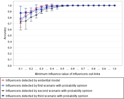
(a) Accuracy of detected influencers while varying the minimum influence value

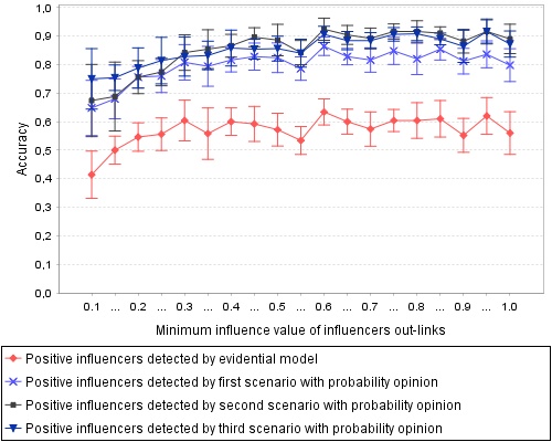
(b) Accuracy of detected positive influencers while varying the minimum influence value

Figure 1: Accuracy variation while varying the minimum influence value

In a second experiment, we vary the “minimum positive opinion” value of influence users in the generated data. In this experiment, we fixed the minimum influence value to 0.5, the minimum positive and negative opinion of positive influencers neighbors to 0.3 and 0.8 respectively. Figure 2 presents the accuracy of detecting influencers having a positive opinion by the mean of each experimented model. In this figure, we notice a similar results to those of the Figure 1b. In fact, all curves are almost steady. Besides, the best accuracy is given by the second, the third and the first scenarios respectively.

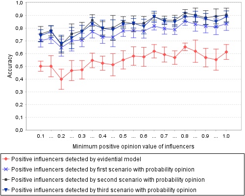
Figure 2: Accuracy of detected positive influencers while varying the minimum positive opinion value

In a third experiment, we vary the “minimum positive opinion of positive influencers neighbors” in the generated data. In this experiment, we fixed the minimum influence value to 0.4, the minimum positive opinion of influencers to 0.5 and the minimum negative opinion of positive influencers neighbors to 0.8. Figure 3 shows the accuracy of detecting positive influencers that exert more influence on positive users. In this figure, we notice a different behavior from the previous figures. In fact, all curves increase gradually when the minimum positive opinion value of positive influencers neighbors increases until getting high accuracy.

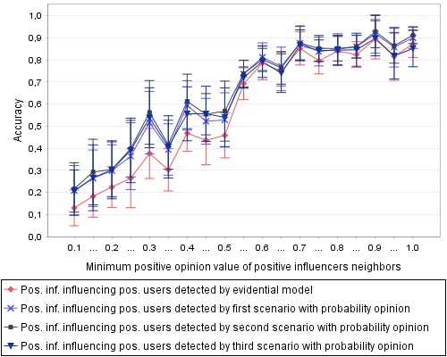
Figure 3: Accuracy of detected positive influencers influencing positive users while varying the minimum positive opinion value of positive influencers neighbors

In a last experiment, we vary the “minimum negative opinion of positive influencers neighbors” in the generated data. Besides, we fix the minimum influence value to 0.4, the minimum positive opinion of influencers to 0.5 and the minimum positive opinion of positive influencers neighbors to 0.2. Figure 4 shows the accuracy of detecting positive influencers that exert more influence on positive and negative users while varying the minimum negative opinion value of positive influencers neighbors. In the first sub-figure 4a, we have the accuracy of detected positive influencers influencing negative users. All curves increase when the varied value increases. Besides, the best accuracy values are given by the third scenario which is dedicated to positive influencers that exert more influence on negative users. In the second sub-figure 4b, we have the accuracy of detected positive influencers influencing positive users. In this figure, we observe a reverse behavior of curves in Figure 4a. In fact, the accuracy decreases when the varied value increases. This behavior is explained by the fact that, when the number of positive influencers influencing negative users increases, the number of those influencing positive users decreases.

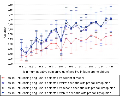
(a) Accuracy of detected positive influencers influencing negative users while varying the minimum negative opinion value of positive influencers neighbors

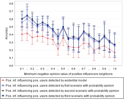
(b) Accuracy of detected positive influencers influencing positive users while varying the minimum negative opinion value of positive influencers neighbors

Figure 4: Accuracy of detected positive influencers influencing positive and negative users while varying the minimum negative opinion value of positive influencers neighbors

To sum up, in this section, we presented some results made on generated data. These results show the adaptability of the used influence maximization model to detect opinion based influencers. Besides, we notice that the results of the first, the second and the third scenarios are similar. This behavior is justified by the similarity between their influence measures.

6 Conclusion

In this paper, we mainly focus on the importance of the user’s opinion when it comes to measuring and maximizing the social influence. In fact, the opinion is a crucial parameter that can determine whether the success or the failure of a viral marketing campaign. To make such a campaign more successful, we introduce three opinion-based viral marketing scenarios. The first scenario is called “positive influencers”, its main aim is to find social influencers having a positive opinion about the product. The second scenario is “positive opinion influencers influencing positive users”, this scenario is about positive influencers that exert more influence on users having a positive opinion. The third scenario is “positive opinion influencers influencing negative opinion users”, it looks for positive influencers that exert more influence on users having a negative opinion. For each scenario, we introduced two appropriate influence measures. Furthermore, we used these measures to maximize the influence. For this purpose, we used an adapted maximization model which is the evidential influence model [15]. Next, we run a set of experiments to show the performance of the proposed solutions. Then, we studied the quality of the detected influencers and their positive and negative opinions using a real world dataset from Twitter network. Besides, we studied the adaptability of the used maximization model to detect the adapted influencers for each scenario and we showed that through a set of experiments on a generated dataset.

An interesting perspective for future works is about maximizing the influence within communities. A community is defined as a set of users or vertices that are connected more densely to each other than to other users from other communities [25, 34, 24]. People in the same community generally have some common properties. For example, they may be friends that attended the same school or they are from the same town. The idea here is to minimize the number of selected influencers and the time spent to find them. In fact, we will search to find influencers at the scale of the community instead of the social network and it is obvious that the community is smaller than the social network.

Siwar Jendoubi is a researcher at LARODEC Laboratory. She received a PhD degree (2016) in computer science and a Master degree (2012) in business intelligence. Dr. Siwar Jendoubi joined the LISTIC Laboratory for 18 months as postdoctoral researcher. Her research interests are mainly related to information fusion, uncertainty management, machine learning, social network analysis and tree species recognition. She is author of many papers.

Arnaud Martin is full professor at University of Rennes 1 in the team DRUID of IRISA laboratory. He received a HDR (French ability to supervised research) in computer sciences (2009), a PhD degree in Signal Processing (2001), and Master in Probability (1998). Pr. Arnaud Martin joined the laboratory IRISA at the university of Rennes 1 as full professor in 2010 and co-create the team DRUID in 2012. He teaches data fusion, data mining, and computer sciences. His research interests are mainly related to the belief functions with applications on social networks and crowdsourcing. He is author of numerous papers and invited talks. He supervised numerous Phd students. Pr. Arnaud Martin is the founder in 2010 of the Belief Functions and Applications Society (BFAS) (www.bfasociety.org). From 2010 until 2012 he was the president of BFAS, and since 2012 he is the treasurer.

References

- [1] Baccianella, S., Esuli, A., Sebatiani, F.: Sentiwordnet 3.0: An enhanced lexical resource for sentiment analysis and opinion mining. In: Proceedings of the Seventh conference on International Language Resources and Evaluation. pp. 2200–2204 (May 2010)
- [2] Barbieri, N., Bonchi, F., Manco, G.: Topic-aware social influence propagation models. Knowledge and Information Systems 37(3), 555–584 (December 2013)
- [3] Baumeister, R., Bratslavsky, E., Finkenauer, C., Vohs, K.: Bad is stronger than good. Review of General Psychology 5(4), 323–270 (2001)
- [4] Chen, D., Lü, L., Shang, M.S., Zhang, Y.C., Zhou, T.: Identifying influential nodes in complex networks. Physica A: Statistical mechanics and its applications 391(4), 1777–1787 (2012)
- [5] Chen, W., Collins, A., Cummings, R., Ke, T., Liu, Z., Rincon, D., Sun, X., Wang, Y., Wei, W., Yuan, Y.: Influence maximization in social networks when negative opinions may emerge and propagate. In: Procedings of SIAM SDM. pp. 379–390 (April 2011)
- [6] Cheung, C.M., Lee, M.K.: Online consumer reviews: Does negative electronic word-of-mouth hurt more? In: Proceeding of the fourteenth americas conference on information systems. p. 143 (August 2008)
- [7] Dempster, A.P.: Upper and Lower probabilities induced by a multivalued mapping. Annals of Mathematical Statistics 38, 325–339 (1967)
- [8] Domingos, P., Richardson, M.: Mining the network value of customers. In: Proceedings of KDD’01. pp. 57–66 (2001)
- [9] Gao, C., Wei, D., Hu, Y., Mahadevan, S., Deng, Y.: A modified evidential methodology of identifying influential nodes in weighted networks. Physica A 392(21), 5490–5500 (November 2013)
- [10] Goldenberg, J., Libai, B., Muller, E.: Talk of the network: A complex systems look at the underlying process of word-of-mouth. Marketing Letters 12(3), 211–223 (August 2001)
- [11] Goyal, A., Bonchi, F., Lakshmanan, L.V.S.: A data-based approach to social influence maximization. In: Proceedings of VLDB Endowment. pp. 73–84 (August 2012)
- [12] Granovetter, M.: Threshold models of collective behavior. American journal of sociology pp. 1420–1443 (1978)
- [13] Jendoubi, S., Chebbah, M., Martin, A.: Evidential independence maximization on twitter network. In: Belief Functions: Theory and Applications, pp. 121–128. Springer International Publishing (2018)
- [14] Jendoubi, S., Martin, A., Liétard, L., Ben Hadj, H., Ben Yaghlane, B.: Maximizing positive opinion influence using an evidential approach. In: Poceeding of the 12th international FLINS conference (August 2016)
- [15] Jendoubi, S., Martin, A., Liétard, L., Ben Hadj, H., Ben Yaghlane, B.: Two evidential data based models for influence maximization in twitter. Knowledge-Based Systems 121, 58–70 (2017)
- [16] Jendoubi, S., Martin, A., Liétard, L., Ben Yaghlane, B.: Classification of message spreading in a heterogeneous social network. In: Proceeding of IPMU. pp. 66–75 (July 2014)
- [17] Jendoubi, S., Martin, A., Liétard, L., Ben Yaghlane, B., Ben Hadj, H.: Dynamic time warping distance for message propagation classification in twitter. In: Proceeding of ECSQARU. pp. 419–428 (July 2015)
- [18] Jurvetson, S.: What exactly is viral marketing? Red Herring 78, 110–112 (2000)
- [19] Kempe, D., Kleinberg, J., Tardos, E.: Maximizing the spread of influence through a social network. In: Proceedings of KDD’03. pp. 137–146 (August 2003)
- [20] Leskovec, J., Krause, A., Guestrin, C., Faloutsos, C., VanBriesen, J., Glance, N.: Cost-effective outbreak detection in networks. In: Proceedings of KDD’07. pp. 420–429 (August 2007)
- [21] Li, D., Xu, Z.M., Chakraborty, N., Gupta, A., Sycara, K., Li, S.: Polarity related influence maximization in signed social networks. PLoS ONE 9(7), e102199 (July 2014)
- [22] Li, Y.M., Lai, C.Y., Chen, C.W.: Discovering influencers for marketing in the blogosphere. Information Sciences 181(23), 5143–5157 (December 2011)
- [23] Liu, Q., Xiang, B., Yuan, N.J., Chen, E., Xiong, H., Zheng, Y., Yang, Y.: An influence propagation view of PageRank. ACM Transactions on Knowledge Discovery from Data 11(3), 1–30 (mar 2017)
- [24] Moosavi, S.A., Jalali, M., Misaghian, N., Shamshirband, S., Anisi, M.H.: Community detection in social networks using user frequent pattern mining. Knowledge and Information Systems 51(1), 159–186 (April 2017)
- [25] Narayanam, R., Nanavati, A.A.: Design of viral marketing strategies for product cross-sell through social networks. Knowledge and Information Systems 39(3), 609–641 (June 2014)
- [26] Newman, M.E.J.: Networks: An introduction. Oxford University Press (2010)
- [27] Shafer, G.: A mathematical theory of evidence. Princeton University Press (1976)
- [28] Smets, P., Kennes, R.: The Transferable Belief Model. Artificial Intelligent 66, 191–234 (1994)
- [29] Taylor, S.E.: Asymmetrical effects of positive and negative events: the mobilization-minimization hypothesis. Psychological bulletin 1(110), 67–85 (1991)
- [30] Wei, D., Deng, X., Zhang, X., Deng, Y., Mahadeven, S.: Identifying influential nodes in weighted networks based on evidence theory. Physica A 392(10), 2564–2575 (Mai 2013)
- [31] Xiang, B., Liu, Q., Chen, E., Xiong, H., Zheng, Y., Yang, Y.: Pagerank with priors: An influence propagation perspective. In: Proceedings of the Twenty-Third International Joint Conference on Artificial Intelligence. pp. 2740–2746 (2013)
- [32] Yang, J., Liu, C., Teng, M., Chen, J., Xiong, H.: A unified view of social and temporal modeling for b2b marketing campaign recommendation. IEEE Transactions on Knowledge and Data Engineering 30(5), 810–823 (may 2018)
- [33] Zhang, H., Dinh, T.N., Thai, M.T.: Maximizing the spread of positive influence in online social networks. In: Proceedings of ICDCS. pp. 317–326 (July 2013)
- [34] Zhou, K., Martin, A., Pan, Q., Liu, Z.g.: Median evidential c-means algorithm and its application to community detection. Knowledge-Based Systems 74, 69–88 (2015)