First search for long-duration transient gravitational waves after glitches in the Vela and Crab pulsars

Abstract

Gravitational waves (GWs) can offer a novel window into the structure and dynamics of neutron stars. Here we present the first search for long-duration quasi-monochromatic GW transients triggered by pulsar glitches. We focus on two glitches observed in radio timing of the Vela pulsar (PSR J0835–4510) on 12 December 2016 and the Crab pulsar (PSR J0534+2200) on 27 March 2017, during the Advanced LIGO second observing run (O2). We assume the GW frequency lies within a narrow band around twice the spin frequency as known from radio observations. Using the fully-coherent transient-enabled $\mathcal{F}$-statistic method, we search for transients of up to four months in length. We find no credible GW candidates for either target, and through simulated signal injections we set 90% upper limits on (constant) GW strain as a function of transient duration. For the larger Vela glitch, we come close to beating an indirect upper limit for when the total energy liberated in the glitch would be emitted as GWs, thus demonstrating that similar post-glitch searches at improved detector sensitivity can soon yield physical constraints on glitch models.

I Introduction

Neutron stars (NSs) provide a rich astrophysical laboratory for nuclear physics at extreme densities. Gravitational waves (GWs) can contribute to probing NS structure and dynamics through observations of binary mergers like GW170817 [1], but also by searching for signals from individual, rapidly spinning objects [2]. One of the most prominent dynamic features of individual NSs is the presence of timing glitches (sudden spin-up events) in pulsars [3]. Glitches are considered promising probes of the NS interior [4, 5, 6] and possible emitters of detectable GW signals [7, 8, 9, 10, 11].

Despite 50 years of glitch observations and a lot of productive model development [12], the mechanism (or mechanisms) behind glitches are not well understood. This is where detecting transient GW signals during or following a glitch could yield valuable insights, as they would directly measure changes in the quadrupole moment of the NS.

So far, the only dedicated analysis of LIGO-Virgo [13, 14] data that touched on this topic was a search for short ($\sim\mathcal{O}$(s)) signals from a 2006 glitch of the Vela pulsar in initial LIGO data [15]. Targeted searches for continuous wave (CW) signals from known pulsars (most recently [16, 17, 18, 19]) have also taken observed glitches into account as breaks in the pulsar ephemerides, but these always focus on persistent signals lasting for the full observation times before/after the glitch. Intermediate-duration transient searches have also been performed on magnetar bursts (most recently in [20] and to look for a post-merger remnant of GW170817 [21, 22], but for those targets the emission mechanisms and parameter space are very different than for pulsar glitches.

Here we perform a dedicated transient analysis of GW data from the Advanced LIGO (aLIGO) second observing run (O2, December 2016 to August 2017), searching for transient GW signals lasting hours to months after two glitches observed from the Vela pulsar (PSR J0835–4510) on 12 December 2016 (MJD $57734.484991\pm 0.000029$ [23, 24, 25]) and the Crab pulsar (PSR J0534+2200) on 27 March 2017 (MJD $57839.92\pm 0.06$, [26, 27]). Due to their relatively young ages and close distances, these were the first two pulsars for which the indirect spin-down upper limit on CW emission (see e.g. Sec. 2.3 of [28]) was beaten [29, 30]. They are not the only known pulsars to have glitched during O2, and targeting a larger sample will be interesting in the future. Sec. 2.2 of [18] gives an overview of known pulsars accessible to LIGO-Virgo searches, though not all are known to glitch; and many known glitching pulsars listed in the standard public catalogues [27, 31] are unfortunately not within the aLIGO sensitivity band. The search presented in this paper is intended as a pilot instance of this new type of transient analysis, and the Crab and Vela pulsars were natural choices as the highest-priority targets.

To this end, we for the first time apply the transient $\mathcal{F}$-statistic method introduced by Prix, Giampanis & Messenger [9] to actual LIGO data. It focuses on long-duration (hours to months) transient GW signals that are quasi-monochromatic, i.e. narrowly localized in frequency (near twice the pulsar’s rotation frequency) at each point during the observation time and slowly evolving in both frequency and amplitude. The data is split into Short Fourier Transforms (SFTs) and then, for a bank of templates from a simple frequency-evolution and transient-window model, a maximum-likelihood matched-filter statistic is computed. The method does not assume a particular glitch model, but only that the GW emission resembles these simple phenomenological templates.

We present the data set used for this study in Sec. II, general aspects of the signal model and $\mathcal{F}$-statistic method in Sec. III and the specific search setup used in Sec. IV. Sec. V summarizes the search results and provides upper limits (ULs) on GW strain under the targeted signal model. In Sec. VI we discuss their implications and an outlook for future applications and refinements of this approach.

II Data used

We use data from the O2 run of the two aLIGO detectors [13] in Hanford (H1) and Livingston (L1). We start from the standard set [32] of 1800 s long Tukey-windowed non-overlapping SFTs used in previous CW searches, e.g. [33]. (See Sec. IV.C.1 of [34] for the general construction of SFTs.) These were produced from the C02 version of calibrated strain data [35, 36, 37] with some subtraction of known noise sources [38, 39]. As detailed in the next section, we use about four months of data for each glitch search (using YYYYMMDD notation for dates in the following): 20161211–20170411 for Vela and 20170327–20170726 for the Crab, covering (3597, 3156) and (2793, 3091) SFTs from (H1,L1) respectively. This corresponds to effective duty factors of (62%, 54%) and (48%, 53%). Coincidence on a per-SFT level is not required for this analysis.

Two periods of O2, of about one month each, of interest to this search have been marked as spectrally contaminated in a single detector [32] and are not included in the standard SFTs: L1 data before 20170104 and H1 data from 20170315–20170418. We have investigated these data ranges in more detail and for the two narrow frequency bands we consider here (around twice the Vela and Crab rotation frequencies), we have found that there are not prohibitively many strong additional contaminations in these months which are not also present in adjacent data. Hence, we have generated additional SFTs for these ranges from frame data publicly available on GWOSC [40], using the script lalapps_MakeSFTDAG [41] with exactly the same settings as for the standard set.

Some additional cleaning of narrow disturbances (‘lines’) was necessary. A detailed list of aLIGO O2 lines of relevance to CW searches, with known instrumental causes, has been provided by [42]; but since we are interested only in two narrow frequency bands and in particular in transient disturbances, we have also performed a separate, simpler but more targeted line identification exercise. Details are given in appendix A.

III Signal model and search method

Following [9], our signal model is a slowly-varying quasi-monochromatic transient

$$h(t,\lambda,\mathcal{A},\mathcal{T})=\varpi(t,t_{0},\tau)\,h(t,\lambda,\mathcal{A})\,,$$ (1)

corresponding to a classic CW signal $h(t,\lambda,\mathcal{A})$ [43] with an additional window function $\varpi(t;t_{0},\tau)$ where the transient parameters $\mathcal{T}$ consist of the window shape, signal start time $t_{0}$ and a duration parameter $\tau$. The CW part depends on a set of phase evolution parameters $\lambda=\{\alpha,\delta,f,{\dot{f}},\ddot{f},\dots\}$ (sky position, frequency, and frequency derivatives or ‘spindowns’) and on four amplitude parameters $\mathcal{A}=\{h_{0},\cos\iota,\psi,\phi_{0}\}$, which our detection statistic (the $\mathcal{F}$-statistic first introduced in [43]) analytically maximizes over. ($h_{0}$: dimensionless amplitude, $\iota$ and $\psi$: orientation and polarization of the source, $\phi_{0}$: GW phase at reference time $T_{\mathrm{ref}}$.) The signal amplitude for a deformed NS at distance $d$, emitting GWs at $f=2f_{\mathrm{spin}}$ in the dominant $l=m=2$ mode from a quadrupolar ellipticity $\epsilon$, with principal moment of inertia $\mathcal{I}$, is given by

$$h_{0}=\frac{4\pi^{2}G}{c^{4}}\frac{\epsilon\,\mathcal{I}}{d}f^{2}\,.$$ (2)

Hence, the simplest interpretation of our transient signal model would be a temporary increase in the quadrupolar deformation after the glitch, with the product $\epsilon\,I$ falling off again as determined by the transient window function with timescale $\tau$. This would be an intuitive behaviour within the ‘starquake’ model of pulsar glitches [44, 45, 46], where the crust is violently deformed. In the more popular class of glitch models based on a rotation lag between the bulk of the NS and an interior superfluid component, the interpretation becomes more complicated, and could involve processes such as crustal heating [47], non-axisymmetric oscillations [8] or post-glitch excitation of Ekman flows [7, 8, 11]. These options are reviewed in more detail in  [9, 12]. For our search, the mechanism does not initially matter as long as a bank of templates from the simple signal model provides a sufficient fit to the real signal. The connection to physical models can be made later, based on the signal durations and amplitudes observed, or from the obtained ULs.

Table 1: Search targets and their key parameters. Much higher-precision sky location $(\alpha,\delta)$ and frequency evolution ($f,{\dot{f}},\ddot{f}$) from the radio ephemerides are used in the search, with a factor 2 to convert from rotation to GW emission rates, and ranges of 0.1 Hz in $f$ and $\approx 10^{-13}$ Hz s^-1 in ${\dot{f}}$ are explored around the nominal values. For the Vela pulsar, all parameters are referenced to MJD 58000, while for the Crab pulsar the position epoch is MJD $\approx 53254$ and the frequency epoch is MJD $\approx 57185.127$. The glitch times $T_{\mathrm{glitch}}$ (in GPS seconds) and glitch sizes $\Delta f/f$ are taken from [27]

target	$d$ [pc]	$\alpha$ [rad]	$\delta$ [rad]	$f$ [Hz]	${\dot{f}}$ [Hz s-1]	$\ddot{f}$ [Hz s-2]	$T_{\mathrm{glitch}}$ [s]	$\Delta f/f$
Vela (J0835–4510)	287 [48]	2.2486	-0.7885	22.3722	$-3.12\cdot 10^{-11}$	$1.16\cdot 10^{-19}$	1165577920	$1.43\cdot 10^{-6}$
Crab (J0534+2200)	2000 [49, 50]	1.4597	-0.3842	59.3295	$-7.39\cdot 10^{-10}$	$1.72\cdot 10^{-20}$	1174687506	$2.14\cdot 10^{-9}$

For each target pulsar, $\alpha$ and $\delta$ are fixed. We place a grid in $(f,{\dot{f}})$ space with fixed spacings. The search method, implemented in the program lalapps_ComputeFstatistic_v2 [41], then loops over this grid, and for each $\lambda=(f,{\dot{f}})$ pair it computes the transient $\mathcal{F}$-statistic map

$$\mathcal{F}_{mn}(\lambda)=\mathcal{F}(\lambda,t_{0\,m},\tau_{n})$$ (3)

by computing partial sums, corresponding to all $\{t_{0\,m},\tau_{n}\}$ combinations, of the per-SFT ‘atomic’ ingredients [9, 51] of the $\mathcal{F}$-statistic. This corresponds to demodulating [52] the detector data over the whole observation time once for each $\lambda$ template, taking into account the time-varying detector response, and then simple arithmetic operations for the transient aspect.

In this search, we use a simple ‘rectangular window’, i.e. $h_{0}=\mathrm{const.}$ for $t\in[t_{0},t_{0}+\tau]$ and $h_{0}=0$ outside. The maximum loss compared to more realistic exponential-decay windows has already been estimated as acceptable in [9]. A search with exponential windows would also be computationally much more costly; see [53] for a detailed discussion. Also see Sec. VI and appendix C for more details on this point.

To obtain detection candidates, we are interested in peaks over the full $(\lambda,\mathcal{T})=(f,{\dot{f}},t_{0},\tau)$ space. To reduce the number of strong $\mathcal{F}$-statistic outliers due to single-detector noise disturbances, we also apply the line-robust statistic $B_{\mathrm{SGL}}$ from [54] at every point, and for each $\lambda$ we only store the values of $\max\limits_{t_{0},\tau}\mathcal{F}_{mn}(\lambda)$ over the subset where $B_{\mathrm{SGL}}(\lambda,t_{0},\tau)$ is above some threshold. In the end, candidates are identified from the $\mathcal{F}$-ordered results, as the $\mathcal{F}$-statistic is directly related to the signal-to-noise ratio (SNR) and its analytically known distribution will allow us to set a detection threshold without additional pure-noise Monte Carlos. $B_{\mathrm{SGL}}$ is thus used here simply as an intermediate veto step, not as a full replacement detection statistic.

IV Search setup and parameter space covered

The key parameters of the two target pulsars and their glitches during O2 are summarized in Table 1. For each glitch, we search for transients starting in a $\Delta t_{0}=1$ day window centred around the nominal glitch epoch and with durations $\tau$ up to 121 days. Hence we search a data set of $T_{\mathrm{obs}}\approx 4$ months, chosen for two reasons:

(i) With the whole of O2 lasting about 9 months, for much longer $\tau$ we would no longer get sufficient benefits from the transient $\mathcal{F}$-statistic over the results of full-O2 CW analyses [18, 19]. From Eq. (62) in [9], the mismatch (relative loss in squared SNR) for observing a signal of true length $\tau_{s}$ with a rectangular template window of length $\tau$ is $m\approx 1-(\tau-\tau_{s})^{2}/(\tau\tau_{s})$. So for a maximum $\tau_{s}=4$ months and a full-O2 CW search’s $\tau=9$ months, we expect $m\approx 30$% corresponding to still about a factor of 2 gain in SNR for a transient with our maximum $\tau$ compared to the full-O2 CW search. For longer $\tau_{s}$, the gain would be correspondingly smaller.

(ii) $T_{\mathrm{obs}}\approx 4$ months also matches the duration of the first aLIGO observing run (O1), so that, at the longest $\tau$, our search becomes comparable in setup to the O1 narrow-band search [17] and we can draw some direct comparisons in the following.

Similar to [17, 19], we allow for some mismatch between the true GW frequency $f$ and its nominal value (twice the radio-observed $f_{\mathrm{spin}}$), constructing a rectangular search grid in $(f,{\dot{f}})$ space. We choose resolutions in GW frequency and spin-down of $df=1/T_{\mathrm{obs}}\approx 9.57\times 10^{-8}$ Hz and $d{\dot{f}}=1/T_{\mathrm{obs}}^{2}\approx 9.15\times 10^{-15}$ Hz s^-1, and cover a frequency range of 0.1 Hz and a spindown range of $11d{\dot{f}}\approx 1.01\times 10^{-13}$ Hz s^-1 both centred on a point $(f,{\dot{f}})$ corresponding to twice the values from the pulsar’s radio ephemerides.

The ephemerides were obtained from observations at the University of Tasmania’s Mount Pleasant Radio Observatory for Vela and at Jodrell Bank (UK) for the Crab, using the TEMPO2 software [55]. Both were originally fitted with the goal of minimal residuals over the whole respective data ranges of the CW searches in [18]. Vela, in addition to glitch recovery, has a lot of timing noise [56, 57] and micro-glitches [58]; hence, to minimize overall residuals, the post-glitch ephemeris for O2 was fitted down to the twelfth derivative (without an exponential recovery term). Thus, and due to the intrinsic rapid evolution of the frequency and its derivatives after a glitch, the $\ddot{f}$ in Table 1 should not be compared directly with the long-time value reported by [59]. Similarly, the Crab pulsar also has significant timing noise and glitch recovery complicating its spin-down [60]. For its O2 ephemeris, no explicit glitch model was used, but again twelve spin-down derivatives were included to minimize overall residuals.

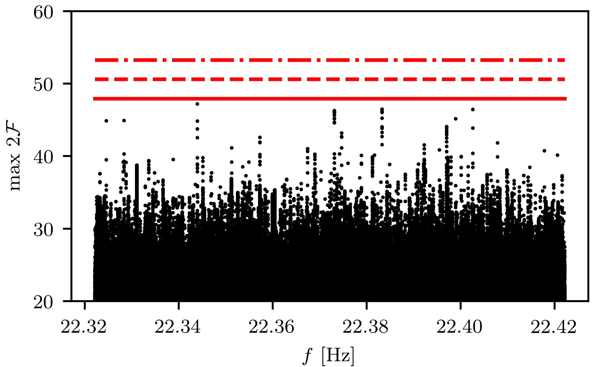
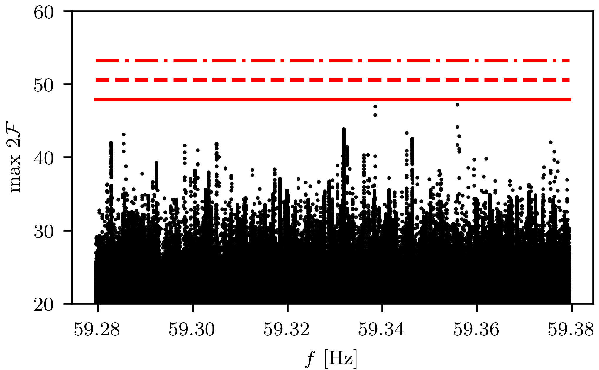
Figure 1: Search results for transients following the 20161212 Vela glitch (left panel) and 20170327 Crab glitch (right panel) with the detection statistic $\max 2\mathcal{F}(f,{\dot{f}})$ maximized over transient parameters $\{t_{0},\tau\}$ and projected onto the $f$ axis. Horizontal lines correspond to expected maximum outliers (and also +1 and +2 standard deviations) for an estimated effective template count (per target) of $5.75\cdot 10^{8}$.

For both targets, we use the $(f,{\dot{f}}$) grid as described above, a single fixed value for $\ddot{f}$, and set higher-order terms to zero, which is valid in the sense that we are accumulating less than a bin of mismatch in $f$ over our $T_{\mathrm{obs}}$ from the second derivative and higher. In addition, while both ephemerides have reference times far from the glitches, the ranges covered in $f$ and ${\dot{f}}$ mean that either we resolve the glitch step with multiple templates (Vela), or the glitch step is itself smaller than our search resolution (Crab), so that extrapolation to around the glitch epoch is safe for the purpose of this search.

The overall frequency evolution template count is $N_{\lambda}=N_{f}N_{\dot{f}}\approx 1.15\times 10^{7}$. Comparing with [17], these choices mean we cover slightly wider ranges in $f$ and ${\dot{f}}$ for Vela while for the Crab we cover the same $f$ and a narrower ${\dot{f}}$ range by a factor 15.

For each $\{f,{\dot{f}}\}$ parameter space point, transient parameters of $t_{0}\in[T_{\mathrm{glitch}}-0.5\,\mathrm{days},T_{\mathrm{glitch}}+0.5\,\mathrm{days}]$ and $\tau\in[0.5\,\mathrm{days},T_{\mathrm{obs}}]$ are analyzed with a resolution $dt_{0}=d\tau=T_{\mathrm{SFT}}=1800$ s, yielding $N_{\mathcal{T}}=N_{t_{0}}N_{\tau}=48\times 5784\approx 2.8\times 10^{5}$ grid points.

The lower limit of $\tau\geq 0.5\,\mathrm{days}$ is chosen empirically to avoid spurious outliers when statistics fluctuate too much over a small number of SFTs. In principle, the transient-$\mathcal{F}$-statistic method can be extended to much shorter $\tau$ but this would require additional copies of the data set with shorter $T_{\mathrm{SFT}}$. This could be done in the future, or a more adaptive multi-timescale approach could be pursued; but for this pilot search we limit ourselves to the standard data set with $T_{\mathrm{SFT}}=1800$ s and correspondingly do not explore very short transients.

The line-robust $B_{\mathrm{SGL}}$ statistic we use as a veto has a free tuning parameter $\mathcal{F}_{*}^{(0)}$ determining how strongly it is allowed to deviate from the standard $\mathcal{F}$-statistic [54]. Since in this search we are dealing with narrow frequency bands which are already known to contain some disturbances, we choose a relatively low value $\mathcal{F}_{*}^{(0)}=10$ corresponding to a statistic that would be slightly suboptimal in purely Gaussian noise but is stricter in suppressing lines. We then set a rather lenient threshold of $B_{\mathrm{SGL}}>-10$ to only cut out very strong single-detector artifacts that might have passed our line cleaning procedure (see appendix A), without severely affecting the distribution of $\mathcal{F}$-statistic values.

V Results

V.1 Search results: no significant candidates

Full results for the $\max 2\mathcal{F}(f,{\dot{f}})$ statistic (maximized over $t_{0}$ and $\tau$), projected onto the frequency axis, are shown in Fig. 1 for both the 20161212 Vela glitch and the 20170327 Crab glitch.

To determine whether the loudest of these per-template results constitute promising detection candidates, we can consider the well-known [e.g. 61] statistical properties of the $\mathcal{F}$-statistic: as $2\mathcal{F}$ in pure Gaussian noise follows a $\chi^{2}_{4}$ distribution (with 4 degrees of freedom), the loudest value $2\mathcal{F}^{*}$ from $N$ independent trials is distributed as

$$p(2\mathcal{F}^{*};N)=N\,\chi^{2}_{4}(2\mathcal{F}^{*})\,\chi^{2}_{4}(2F<2\mathcal{F}^{*})^{N-1}\,,$$ (4)

where $\chi^{2}_{4}(2\mathcal{F}^{*})$ is the probability distribution function evaluated at $2\mathcal{F}^{*}$ and $\chi^{2}_{4}(2F<2\mathcal{F}^{*})$ is the cumulative distribution function integrated up to $2\mathcal{F}^{*}$.

For this search, we need to consider the loudest overall outlier $2\mathcal{F}^{*}=\max_{f,{\dot{f}}}(\max_{t_{0},\tau}2\mathcal{F})$ for each target. Since the $(t_{0},\tau$) templates at each $(f,{\dot{f}})$ point re-use the same data atoms many times, the total effective number of templates is much lower than $N_{\lambda}\cdot N_{\mathcal{T}}$. We find acceptable fits to the $\max 2F$ distribution (over all $(f,{\dot{f}})$) for $N_{\mathcal{T}}^{\mathrm{eff}}\approx 50$, and then use a total $N^{\mathrm{eff}}\approx 50\cdot N_{\lambda}$ to obtain (numerically from Eq. 4) an expectation value $E[2\mathcal{F}^{*}]\approx 48$ with standard deviation $\sigma[2\mathcal{F}^{*}]\approx 2.7$.

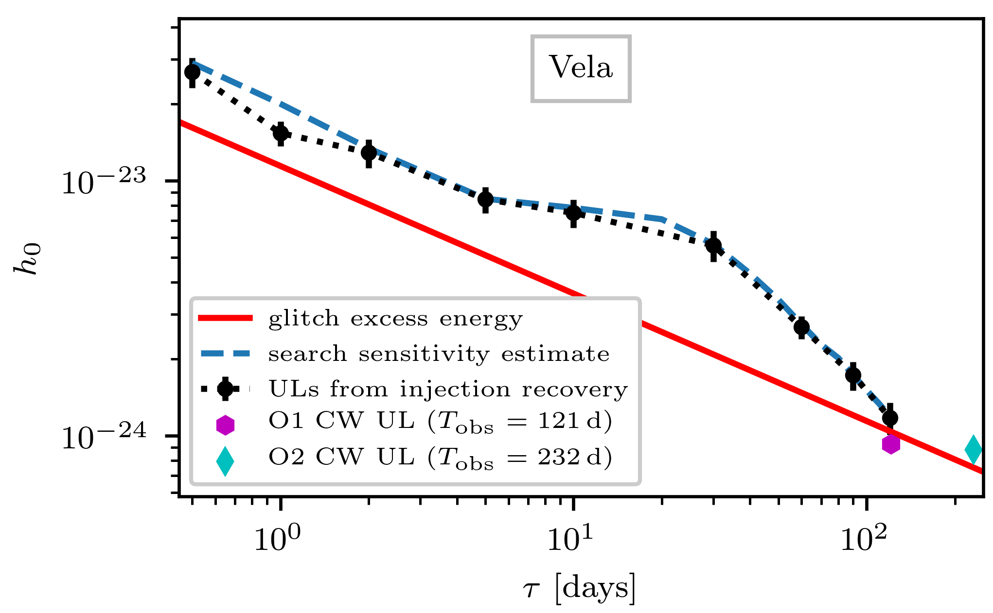
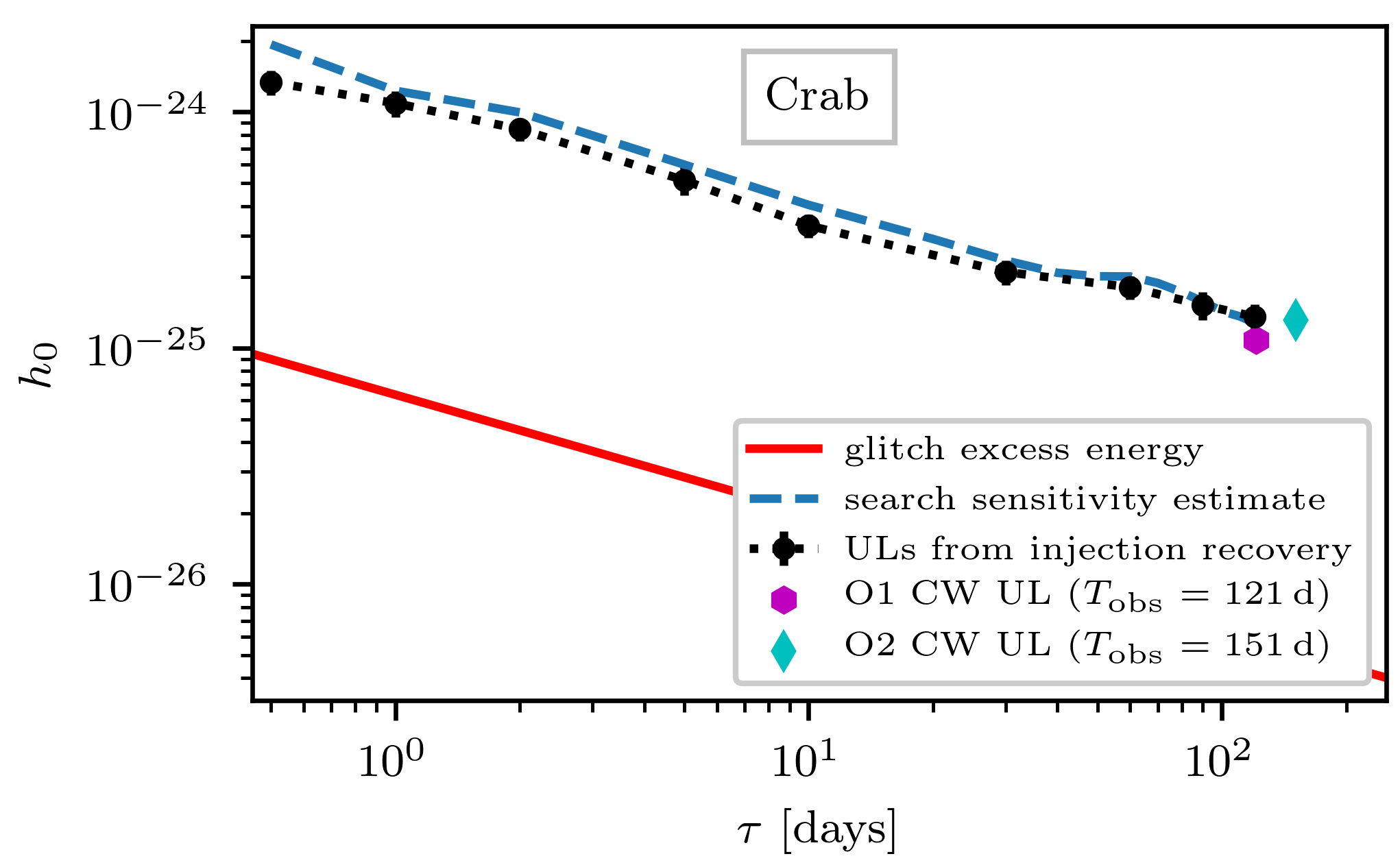
Figure 2: ULs on GW strain for transients following the 20161212 Vela glitch (left panel) and 20170327 Crab glitch (right panel) as a function of the duration $\tau$ of rectangular-windowed signals. The black points and dotted lines represent our ULs at 90% confidence from simulated signal injections randomized over all other parameters. Error bars are estimated from a sigmoid fit to $p_{\mathrm{det}}(h_{0})$ curves, with a small contribution from calibration uncertainty (see appendix B). For comparison, we also show the glitch excess energy indirect ULs from Eq. 5 (solid red lines), a semi-analytic sensitivity estimate for the search (dashed blue lines) and the ULs for persistent CWs previously obtained in [17] (magenta hexagons, full O1 data) and [19] (cyan diamonds, O2 data starting 20170104 for Vela and after 20170327 for the Crab).

The loudest candidate from the Vela search has $2\mathcal{F}^{*}\approx 47.19$, and from the Crab search the loudest outlier is at $2\mathcal{F}^{*}\approx 47.18$. These do not even cross a nominal $E[2\mathcal{F}^{*}]\approx 48$ threshold, which might be considered a low-level criterion for further follow-up study. And even though the precise threshold to put could be shifted somewhat when revisiting the assumptions in effective template counting, any truly promising candidate would need to lie a few standard deviations above expectation. For comparison, levels of $E$, $E+\sigma$ and $E+2\sigma$ are indicated by horizontal lines in Fig. 1.

Hence, while there is some evident substructure in the search results that could be further investigated by follow-ups with different $T_{\mathrm{SFT}}$, gridless MCMC [62] or through more detailed data quality studies, we conclude that the loudest candidates from both targets are so weak that no such effort is warranted at this point. We proceed next to set ULs on GW strain from our targets based on the absence of a detection.

V.2 Upper Limits

To obtain ULs on the emitted strain from/after the two targeted glitches, still under the simplified assumption of a ‘rectangular’ transient, we perform software injections of simulated signals into the same data sets as used for the original searches, and determine the required scale of $h_{0}$ at which 90% of signals are recovered above the nominal $E[2\mathcal{F}^{*}]\approx 48$ threshold. Physically, for a fixed overall energy budget of the glitch we would expect lower $h_{0}$ for longer $\tau$. At the same time, our search sensitivity also improves roughly with $\sqrt{\tau}$. Hence, we present ULs on $h_{0}$ as a function of $\tau$, randomizing over all other parameters. Details on the procedure are given in appendix B, and the results are shown in Fig. 2.

In the same figures, we also compare the measured ULs against a sensitivity estimate for our search based on the octapps [63] CW sensitivity calculator (see [64] for a detailed description). To obtain this curve, we consider CW-like searches over a grid in $T_{\mathrm{obs}}=\tau$ and feed the estimation code with cumulative duty factors and harmonic-mean averages of the detector power spectral density (PSD) over each of these durations, as well as an estimated average mismatch of 0.2 for our $(f,{\dot{f}})$ grid and a $2\mathcal{F}$ threshold of 48 as above. The agreement is remarkably close.

We also find that at the longest signal duration probed ($\tau=120$ d) our ULs approach those from the LIGO-Virgo narrow-band searches for CWs from the same targets (see Table VI of [17] and Table IV of  [19]).

VI Discussion

In the absence of significant GW detection candidates after the two glitches in the Vela and Crab pulsars during the aLIGO O2 run, we have set ULs on the emitted GW strain as a function of signal duration $\tau$. To check how physically constraining these ULs are, we consider an indirect transient energy UL in analogy to the well-known spin-down limit from the CW case (see e.g. Sec. 2.3 of [28]). Here we briefly summarize the derivation of this indirect UL from Sec. II.C of [9].

According to the basic two-fluid model of NS glitches (see e.g. [65]), in an intra-glitch period the bulk of the NS gradually spins down, while an interior superfluid component retains most of its initial angular momentum. Then assuming (i) a glitch transfers the whole angular momentum difference previously built up between the two components, (ii) the moments of inertia $\mathcal{I}_{\mathrm{s}}$ (superfluid) and $\mathcal{I}_{\mathrm{c}}$ (bulk) do not change during the glitch, and (iii) $\mathcal{I}_{\mathrm{s}}\ll\mathcal{I}_{\mathrm{c}}$, then the excess superfluid energy liberated in this transfer is $E_{\mathrm{glitch}}\approx 4\pi^{2}\,\mathcal{I}_{\mathrm{s}}\,f\Delta_{\mathrm{s-c}}$, where $\Delta_{\mathrm{s-c}}$ is the lag (built-up difference in $f$) between the two components right before the glitch ($\Delta\nu$ in the notation of [9]).

If we further assume that (iv) all of $E_{\mathrm{glitch}}$ is emitted in GWs, and rewrite in terms of the observed relative frequency change $\Delta f/f$ at the glitch and total moment of inertia $\mathcal{I}\approx\mathcal{I}_{\mathrm{c}}$, then the total emitted GW energy is independent of the signal duration $\tau$, while the corresponding GW strain as a function of $\tau$ is

$$h_{0}=\frac{1}{d}\sqrt{\frac{5G}{2c^{3}}\frac{\mathcal{I}}{\tau}\frac{\Delta f}{f}}\,.$$ (5)

As per [9], qualitatively similar ULs still hold for alternative glitch models such as crust-cracking starquakes [46], where instead the moment of inertia of the crust would change at the glitch.

This indirect UL is shown for comparison with our empirical ULs in Fig. 2. For this, we assume a fiducial value of $\mathcal{I}=10^{38}$ kg m² and distances of 287 pc for the Vela pulsar [48] and 2 kpc for the Crab pulsar [49, 50].

With a frequency change of $\Delta f/f=1.431\cdot 10^{-6}$, the Vela glitch was much larger than the Crab glitch with $\Delta f/f=2.14\cdot 10^{-9}$ (both values from [27]; [66] recently suggested a larger initial frequency overshoot in the Vela glitch, which however has already decayed at the timescales probed in this search). Hence, though aLIGO sensitivity is better at the higher of the two target frequencies, for the Crab glitch our O2 search was still far away from the indirect energy UL; while for Vela we got very close to beating it at the shortest and longest $\tau$. Overall, the search sensitivity was mostly limited by the significant time variation of detector sensitivities and duty factors. For example, the slow improvement in Vela ULs at intermediate durations (10–30 days) is largely due to the winter holiday break in O2 observing which made cumulative duty factors drop over this period.

Since the search presented in this paper is the first practical application of the transient-$\mathcal{F}$-statistic method from [9] to GW detector data, we have made several choices to simplify the search setup and post-processing, but which can be improved over in future applications. Notably, the simple rectangular transient window allows for efficient computation, but while it does also recover most of the SNR for different signal shapes (see [9] and appendix C), a more general and sensitive analysis will be possible when including e.g. exponentially decaying window functions. (A natural choice considering the observed exponential recoveries in pulsar frequency after most glitches, see e.g. [67].) Since exponential templates are much more costly, using graphics processing units (GPUs) for the search would be highly beneficial [53].

The search setup can be improved in several other ways, including multi-timescale approaches: i.e. the use of input data at several different SFT durations to cover shorter transients; and varying the metric-based [68] frequency and spin-down resolutions as a function of $\tau$.

To deal with outliers from either detector noise features or actual GW signals, MCMC-based follow-up [62] is a promising technique. If necessary, the detector noise can also be studied in much more detail than was required for this pilot search, e.g. using correlations with auxilliary channels to veto instrumental lines [42]. We also used only an ad-hoc veto version of the line-robust statistic from [54], while a semi-coherent transient-aware version [69] or a customized coherent version would offer the potential for more robust suppression of single-detector instrumental artifacts.

In addition to these improvements in the analysis method, the improved sensitivity and increased number of detectors in O3 (which has started in April 2019) and beyond [70] will be the strongest driver in bringing search results for future pulsar glitches into the physically constraining regime. Since the search method is computationally cheap (already on regular CPUs for rectangular windows, and when using GPUs [53] this stays true also for exponential windows), with some more automation of the analysis pipeline it should be possible to target not only the highest-value objects such as the Vela and the Crab, but more of the large population of glitching pulsars [3].

Appendix A Data cleaning

To identify single-detector noise artifacts in the form of narrow disturbances (spectral lines) within the analysis bands for each pulsar, we have considered a standard quantity for such data quality studies, the normalized SFT power [34]:

$$\mathcal{P}^{X}(f_{k})=\frac{2}{N_{\mathrm{SFT}}\,T_{\mathrm{SFT}}}\frac{\left|\widetilde{x}_{\alpha}^{X}(f_{k})\right|^{2}}{S_{\mathrm{n}}^{X\alpha}(f_{k})}\,.$$ (6)

Here, $\widetilde{x}_{\alpha}^{X}(f)$ is the data in bin $f_{k}$ of the $\alpha^{\mathrm{th}}$ SFT for detector $X$ and $S_{\mathrm{n}}^{X\alpha}(f_{k})$ is a running-median noise PSD estimate. This is computed for the bands in question using the lalapps_ComputePSD tool [41]. We then identified as (possibly transient) single-detector line features those frequency bins (or small number of adjacent bins) where at least 5 SFTs (not necessarily consecutive) crossed a threshold $\mathcal{P}^{X}(f_{k})>10$. These are listed in Table 2. For safety, we would not have vetoed any features common to both detectors – as could be produced by an (extremely loud) astrophysical signal – through this procedure. No such coincident features were found in the two bands.

Comparing with the detailed detector characterization approach of line hunting in [42], we find that the three easily identified H1 artifacts match up with harmonics of known instrumental frequency combs. On the other hand, the three L1 artifacts are all very short and limited to the first month of O2 when an improperly connected ethernet cable induced electronic crosstalk in the interferometer controls system, a period which has not been used in the LIGO-Virgo flagship CW searches [18, 19, 33]. These artifacts do not match any lines or combs listed in [42]. We have not investigated in any more detail whether these additional narrow and transient disturbances are clearly correlated with auxilliary channels, but since they are clearly limited to a single detector, they can still be considered safe for removal from the input data.

Using this list, we have cleaned the input SFTs of the affected detector by replacing the listed bins with samples drawn from a Gaussian distribution with variance matching the surrounding PSD estimate, using lalapps_SFTclean.

After this removal, no outliers with multi-detector $\max 2\mathcal{F}\geq 48$ or single-detector $\max 2\mathcal{F}\geq 52$ are found by the search. So while some of the remaining substructures visible in Fig. 1 are likely due to unidentified narrow instrumental disturbances, possibly including the December 2016 L1 and March–April 2017 H1 issues, none of these are strong enough to lead to significant outliers.

Table 2: Single-detector lines identified through outliers in the normalized SFT power and subsequently removed from the input SFTs for the $\mathcal{F}$-statistic analyses. The more common cases where single bins in a single SFT exceed the threshold are not used for any cleaning. The width is given in terms of the number of bins $N_{\mathrm{bins}}$ at resolution $1/T_{\mathrm{SFT}}=1/1800$ s. The duration is quoted as between the first and last SFT with $\mathcal{P}^{X}(f_{k})\geq 10$, not necessarily meaning that the line is persistently visible during this range, and not excluding that it is still present at a weaker level before and after. For simplicity and safety, the full set of SFTs is cleaned at these frequencies, not just the listed duration. Where the frequency matches up with a harmonic of a known comb of disturbances, the corresponding comb spacing is listed.

detector	$f_{\mathrm{start}}$	$N_{\mathrm{bins}}$	duration	comb [Hz]
H1	22.2222	3	20161202–20170508	11.1111 [42]
H1	22.2500	1	20170204–20170418	0.9999862 [42]
L1	22.3600	3	20161214	unidentified
L1	22.4156	3	20161210–20170104	2.24154 [71, 72]
L1	22.4706	1	20161213	unidentified
H1	59.2733	3	on/off through O2	0.9878881 [42]

Appendix B Details on UL procedure

To obtain the GW strain ULs as a function of signal length $\tau$ as presented in Sec. V.2, we perform software injections of simulated signals into the same input SFTs as used for the main search. At each sample value of $\tau$, we use the lalapps_MakeFakeData_v5 program [41] to simulate a set of signals with varying $h_{0}$, uniformly distributed over the whole search range in $\{f,{\dot{f}},t_{0}\}$ and also randomized over the remaining amplitude parameters $\{\cos\iota,\psi,\phi_{0}\}$. For each injection, a reduced parameter space covering $10^{-4}$ Hz in frequency (with the same $df$ as before) and only 1 spin-down bin is re-analyzed. We count an injection as recovered if it produces $\max 2\mathcal{F}\geq 48$, as a candidate above this nominal threshold would have been considered for further follow-up if found in the main search.

For each $\tau$, the result is then an efficiency curve of detection probability $p_{\mathrm{det}}$ against injected $h_{0}$. This can be fit with a sigmoid

$$p_{\mathrm{det}}(h_{0})=\frac{1}{1+\exp[-a(h_{0}-b)]}$$ (7)

(using scipy.curve_fit) and evaluated at $p_{\mathrm{det}}=0.9$ to estimate a $h_{0}^{90\%}$ UL at 90% confidence. The error on $h_{0}^{90\%}$ is obtained from error propagation of the uncertainties in the fit coefficients $(a,b)$. We have run a relatively small set of UL simulations: 50 injections each at 10–20 $h_{0}$ steps per $\tau$ value, leading to $\sim 10$% uncertainty in $h_{0}^{90\%}$ as evaluated from the fit. An additional contribution comes from calibration uncertainty in the measured strain at the detector [35, 36]. According to [37], for the 20–100 Hz band during O2 the amplitude uncertainties are 1.6% for H1 and 3.9% for L1.

Appendix C Sensitivity compared with exponentially decaying transients

In this search we have only considered the simplest model for quasi-monochromatic transients, i.e. CW-like signals turning on at some time $t_{0}$ and off again at $t_{0}+\tau$ with fixed amplitude, hence referred to as rectangular-windowed signals. The detection method as introduced by [9] however can also deal with more general transient window functions, and as an explicit example the implementations in LALSuite [41] and pyFstat [53] also include transients with exponentially decaying amplitude. Since pulsar rotation frequencies after glitches often show an exponential recovery profile [67], exponential transient windows could be a more realistic option. Here we briefly investigate the effect of trying to recover exponentially-decaying signals with rectangular search windows.

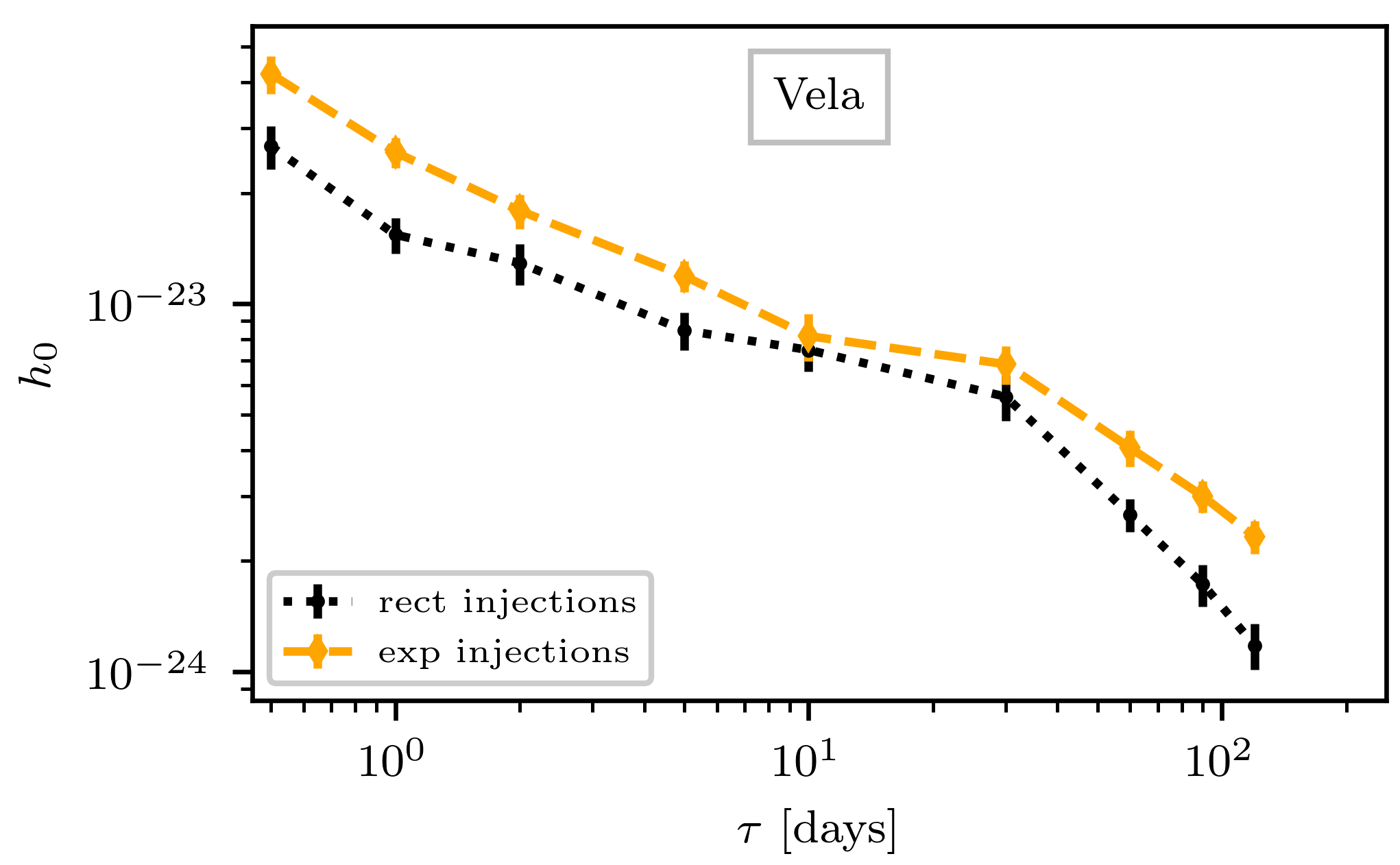
Figure 3: Injection recovery results for the Vela search, comparing transient injections with rectangular window function (black dotted line, same as in Fig. 2) and exponential window function (orange dashed line), both recovered with rectangular search windows.

This question was previously addressed in Sec. V.B of [9] through looking at detection probability $p_{\mathrm{det}}$ against false-alarm probability $p_{\mathrm{fa}}$ for synthetic noise and signal draws. They found moderate losses with a worst case of $\lesssim 10\%$ at relatively high $p_{\mathrm{fa}}$.

As a specific test with more direct relation to the analysis in this paper, let us revisit the UL injection-and-recovery procedure with exponential-window injections. Direct comparison of recovering these injections with both rectangular and exponential search windows is too expensive for the present purpose; instead, we have simply tested the recovery of exponential injections with rectangular search windows – though only for the 20161212 Vela glitch as an example target. Results are shown in Fig. 3, showing that there is indeed some loss in sensitivity from transient window mismatch, and that a dedicated exponential-window search (likely on GPUs [53]) can be valuable in the future. But for the moment, this test also demonstrates that our simplified pilot search also had sensitivity to exponentially decaying signals, with slightly higher ULs as per Fig. 3.

It is worth noting that, following the conventions of [9], the length of an exponential signal with $h_{0}(t)\propto\exp[-(t-t_{0})/\tau]$ is longer than that of a rectangular window with fixed length $\tau$: the initial amplitude falls to 37% after $1\tau$, 14% after $2\tau$ and 5% after $3\tau$, at which point the LALSuite implementation cuts off the window. Hence, one cannot directly compare $p_{\mathrm{det}}$ at a fixed $\tau$ for injections of both window types and purely attribute the difference to window mismatch.

References

- Abbott et al. [2017a] B. P. Abbott et al. (LIGO Scientific Collaboration and Virgo Collaboration), GW170817: Observation of Gravitational Waves from a Binary Neutron Star Inspiral, Phys. Rev. Lett. 119, 161101 (2017a), arXiv:1710.05832 [gr-qc] .
- Glampedakis and Gualtieri [2019] K. Glampedakis and L. Gualtieri, Gravitational waves from single neutron stars: an advanced detector era survey, in The Physics and Astrophysics of Neutron Stars, Astrophys. Space Sci. Libr., Vol. 457, edited by L. Rezzolla, P. Pizzochero, D. I. Jones, N. Rea, and I. Vidaña (Springer, Cham, 2019) pp. 673–736, arXiv:1709.07049 [astro-ph.HE] .
- Fuentes et al. [2017] J. R. Fuentes, C. M. Espinoza, A. Reisenegger, B. W. Stappers, B. Shaw, and A. G. Lyne, The glitch activity of neutron stars, Astron. Astrophys. 608, A131 (2017), arXiv:1710.00952 [astro-ph.HE] .
- Link et al. [1992] B. Link, R. I. Epstein, and K. A. Van Riper, Pulsar glitches as probes of neutron star interiors, Nature 359, 616 (1992).
- Link et al. [2000] B. Link, R. I. Epstein, and J. M. Lattimer, Probing the neutron star interior with glitches, in Stellar Astrophysics - Proc. Pacific Rim Conf., Hong Kong, 1999, Astrophys. Space Sci. Lib., Vol. 254, edited by Cheng, K. S. and Chau, H. F. and Chan, K. L. and Leung, K. C. (Springer, Dordrecht, 2000) pp. 117–126, arXiv:astro-ph/0001245 [astro-ph] .
- Haskell [2017] B. Haskell, Probing neutron star interiors with pulsar glitches, in Symposium 337, Pulsar Astrophysics - The Next 50 Years, Proc. IAU, Vol. 13 (Cambridge University Press, 2017) arXiv:1712.01547 [astro-ph.HE] .
- van Eysden and Melatos [2008] C. A. van Eysden and A. Melatos, Gravitational radiation from pulsar glitches, Class. Quant. Grav. 25, 225020 (2008), arXiv:0809.4352 [gr-qc] .
- Bennett et al. [2010] M. F. Bennett, C. A. van Eysden, and A. Melatos, Continuous-wave gravitational radiation from pulsar glitch recovery, Mon. Not. R. Astron. Soc. 409, 1705 (2010), arXiv:1008.0236 [astro-ph.SR] .
- Prix et al. [2011] R. Prix, S. Giampanis, and C. Messenger, Search method for long-duration gravitational-wave transients from neutron stars, Phys. Rev. D 84, 023007 (2011), arXiv:1104.1704 [gr-qc] .
- Melatos et al. [2015] A. Melatos, J. A. Douglass, and T. P. Simula, Persistent Gravitational Radiation From Glitching Pulsars, Astrophys. J. 807, 132 (2015).
- Singh [2017] A. Singh, Gravitational Wave transient signal emission via Ekman Pumping in Neutron Stars during post-glitch relaxation phase, Phys. Rev. D 95, 024022 (2017), LIGO-P1600091, arXiv:1605.08420 [gr-qc] .
- Haskell and Melatos [2015] B. Haskell and A. Melatos, Models of Pulsar Glitches, Int. J. Mod. Phys. D24, 1530008 (2015), arXiv:1502.07062 [astro-ph.SR] .
- Aasi et al. [2015] J. Aasi et al. (LIGO Scientific Collaboration), Advanced LIGO, Class. Quant. Grav. 32, 074001 (2015), arXiv:1411.4547 [gr-qc] .
- Acernese et al. [2015] F. Acernese et al. (Virgo Collaboration), Advanced Virgo: a second-generation interferometric gravitational wave detector, Class. Quant. Grav. 32, 024001 (2015), arXiv:1408.3978 [gr-qc] .
- Abadie et al. [2011a] J. Abadie et al. (LIGO Scientific Collaboration), A search for gravitational waves associated with the August 2006 timing glitch of the Vela pulsar, Phys. Rev. D 83, 042001 (2011a), arXiv:1011.1357 [gr-qc] .
- Abbott et al. [2017b] B. P. Abbott et al. (LIGO Scientific, Virgo), First search for gravitational waves from known pulsars with Advanced LIGO, Astrophys. J. 839, 12 (2017b), [Erratum: Astrophys. J.851,no.1,71(2017)], arXiv:1701.07709 [astro-ph.HE] .
- Abbott et al. [2017c] B. P. Abbott et al. (Virgo, LIGO Scientific), First narrow-band search for continuous gravitational waves from known pulsars in advanced detector data, Phys. Rev. D 96, 122006 (2017c), arXiv:1710.02327 [gr-qc] .
- Abbott et al. [2019a] B. P. Abbott et al. (LIGO Scientific Collaboration and Virgo Collaboration), Searches for Gravitational Waves from Known Pulsars at Two Harmonics in 2015-2017 LIGO Data, Astrophys. J. 879, 10 (2019a), arXiv:1902.08507 [astro-ph.HE] .
- Abbott et al. [2019b] B. P. Abbott et al. (LIGO Scientific Collaboration and Virgo Collaboration), Narrow-band search for gravitational waves from known pulsars using the second LIGO observing run, Phys. Rev. D 99, 122002 (2019b), arXiv:1902.08442 [gr-qc] .
- Abbott et al. [2019c] B. P. Abbott et al. (LIGO Scientific Collaboration and Virgo Collaboration), Search for Transient Gravitational-wave Signals Associated with Magnetar Bursts during Advanced LIGO’s Second Observing Run, Astrophys. J. 874, 163 (2019c), arXiv:1902.01557 [astro-ph.HE] .
- Abbott et al. [2017d] B. P. Abbott et al. (LIGO Scientific Collaboration and Virgo Collaboration), Search for Post-merger Gravitational Waves from the Remnant of the Binary Neutron Star Merger GW170817, Astrophys. J. Lett. 851, L16 (2017d), arXiv:1710.09320 [astro-ph.HE] .
- Abbott et al. [2019d] B. P. Abbott et al. (LIGO Scientific Collaboration and Virgo Collaboration), Search for gravitational waves from a long-lived remnant of the binary neutron star merger GW170817, Astrophys. J. 875, 160 (2019d), arXiv:1810.02581 [gr-qc] .
- Palfreyman [2016] J. Palfreyman, Glitch observed in the Vela Pulsar (PSR J0835-4510), Astron. Telegram 9847 (2016).
- Sarkissian et al. [2017] J. M. Sarkissian, J. E. Reynolds, G. Hobbs, and L. Harvey-Smith, One year of monitoring the Vela pulsar using a Phased Array Feed, Publ. Astron. Soc. Austral. 34, e027 (2017), arXiv:1705.08355 [astro-ph.HE] .
- Palfreyman et al. [2018] J. Palfreyman, J. M. Dickey, A. Hotan, S. Ellingsen, and W. van Straten, Alteration of the magnetosphere of the Vela pulsar during a glitch, Nature 556, 219 (2018).
- Lyne, A. G. and Roberts, M. E. and Jordan, C. A. [2018] Lyne, A. G. and Roberts, M. E. and Jordan, C. A., Jodrell Bank Crab Pulsar Timing Results – Monthly Ephemeris February 23, 2018, Tech. Rep. (2018).
- Espinoza et al. [2019] C. M. Espinoza et al., Jodrell Bank Pulsar Glitch Catalogue, http://www.jb.man.ac.uk/pulsar/glitches.html (2019).
- Prix [2009a] R. Prix (for the LIGO Scientific Collaboration), Gravitational Waves from Spinning Neutron Stars, in Neutron Stars and Pulsars, Astrophys. Space Sci. Lib., Vol. 357, edited by W. Becker (Springer, Berlin Heidelberg, 2009) Chap. 24, pp. 651–685.
- Abbott et al. [2008] B. Abbott et al. (LIGO Scientific Collaboration), Beating the spin-down limit on gravitational wave emission from the Crab pulsar, Astrophys. J. Lett. 683, L45 (2008), [Erratum: Astrophys. J.706,L203(2009)], arXiv:0805.4758 [astro-ph] .
- Abadie et al. [2011b] J. Abadie et al. (LIGO Scientific Collaboration and Virgo Collaboration), Beating the spin-down limit on gravitational wave emission from the Vela pulsar, Astrophys. J. 737, 93 (2011b), arXiv:1104.2712 [astro-ph.HE] .
- [31] G. B. Hobbs, R. N. Manchester, and L. Toomey, The Australia Telescope National Facility Pulsar Catalogue: Glitch Parameters, https://www.atnf.csiro.au/people/pulsar/psrcat/glitchTbl.html.
- E. Goetz [2019] E. Goetz (for the LIGO Scientific Collaboration and the Virgo Collaboration), Segments used for creating standard SFTs in O2 data, Tech. Rep. LIGO-T1900085 (2019).
- Abbott et al. [2019e] B. P. Abbott et al. (LIGO Scientific Collaboration and Virgo Collaboration), All-sky search for continuous gravitational waves from isolated neutron stars using Advanced LIGO O2 data, Phys. Rev. D 100, 024004 (2019e), arXiv:1903.01901 [astro-ph.HE] .
- Abbott et al. [2004] B. Abbott et al. (LIGO Scientific Collaboration), Setting upper limits on the strength of periodic gravitational waves using the first science data from the GEO 600 and LIGO detectors, Phys. Rev. D 69, 082004 (2004), arXiv:gr-qc/0308050 [gr-qc] .
- Cahillane et al. [2017] C. Cahillane, J. Betzwieser, D. A. Brown, E. Goetz, E. D. Hall, K. Izumi, S. Kandhasamy, S. Karki, J. S. Kissel, G. Mendell, R. L. Savage, D. Tuyenbayev, A. Urban, A. Viets, M. Wade, and A. J. Weinstein, Calibration uncertainty for Advanced LIGO’s first and second observing runs, Phys. Rev. D 96, 102001 (2017), arXiv:1708.03023 [astro-ph.IM] .
- Viets et al. [2018] A. Viets et al., Reconstructing the calibrated strain signal in the Advanced LIGO detectors, Class. Quant. Grav. 35, 095015 (2018), arXiv:1710.09973 [astro-ph.IM] .
- Cahillane et al. [2018] C. Cahillane, M. Hulko, J. S. Kissel, et al., O2 C02 Calibration Uncertainty, Tech. Rep. LIGO-G1800319 (2018).
- Driggers et al. [2019] J. C. Driggers et al. (LIGO Scientific Collaboration), Improving astrophysical parameter estimation via offline noise subtraction for Advanced LIGO, Phys. Rev. D 99, 042001 (2019), arXiv:1806.00532 [astro-ph.IM] .
- Davis et al. [2019] D. Davis, T. J. Massinger, A. P. Lundgren, J. C. Driggers, A. L. Urban, and L. K. Nuttall, Improving the Sensitivity of Advanced LIGO Using Noise Subtraction, Class. Quant. Grav. 36, 055011 (2019), arXiv:1809.05348 [astro-ph.IM] .
- Gravitational Wave Open Science Center [2019] Gravitational Wave Open Science Center (LIGO Scientific Collaboration and Virgo Collaboration), Advanced LIGO O2 Data Release (2019).
- LIGO Scientific Collaboration [2019] LIGO Scientific Collaboration, LIGO Algorithm Library - LALSuite, free software (GPL) (2019).
- Covas et al. [2018] P. B. Covas et al. (LSC), Identification and mitigation of narrow spectral artifacts that degrade searches for persistent gravitational waves in the first two observing runs of Advanced LIGO, Phys. Rev. D 97, 082002 (2018), arXiv:1801.07204 [astro-ph.IM] .
- Jaranowski et al. [1998] P. Jaranowski, A. Królak, and B. F. Schutz, Data analysis of gravitational-wave signals from spinning neutron stars: The signal and its detection, Phys. Rev. D 58, 063001 (1998), arXiv:gr-qc/9804014 [gr-qc] .
- Ruderman [1969] M. Ruderman, Neutron Starquakes and Pulsar Periods, Nature 223, 597 (1969).
- Smoluchowski [1970] R. Smoluchowski, Frequency of Pulsar Starquakes, Phys. Rev. Lett. 24, 923 (1970).
- Middleditch et al. [2006] J. Middleditch, F. E. Marshall, Q. D. Wang, E. V. Gotthelf, and W. Zhang, Predicting the Starquakes in PSR J0537-6910, Astrophys. J. 652, 1531 (2006), arXiv:astro-ph/0605007 [astro-ph] .
- van Riper et al. [1991] K. A. van Riper, R. I. Epstein, and G. S. Miller, Soft X-ray pulses from neutron star glitches, Astrophys. J. Lett. 381, L47 (1991).
- Dodson et al. [2003] R. Dodson, D. Legge, J. E. Reynolds, and P. M. McCulloch, The Vela pulsar’s proper motion and parallax derived from VLBI observations, Astrophys. J. 596, 1137 (2003), arXiv:astro-ph/0302374 [astro-ph] .
- Trimble [1973] V. Trimble, The Distance to the Crab Nebula and NP 0532, Publ. Astron. Soc. Pac. 85, 579 (1973).
- Kaplan et al. [2008] D. L. Kaplan, S. Chatterjee, B. M. Gaensler, and J. Anderson, A Precise Proper Motion for the Crab Pulsar, and the Difficulty of Testing Spin-Kick Alignment for Young Neutron Stars, Astrophys. J. 677, 1201 (2008), arXiv:0801.1142 [astro-ph] .
- Prix [2009b] R. Prix, The F-statistic and its implementation in ComputeFStatistic_v2, Tech. Rep. LIGO-T0900149-v6 (2009) last updated 2018.
- Williams and Schutz [1999] P. R. Williams and B. F. Schutz, An Efficient matched filtering algorithm for the detection of continuous gravitational wave signals, Gravitational waves. Proceedings, 3rd Edoardo Amaldi Conference, Pasadena, USA, July 12-16, 1999, AIP Conf. Proc. 523, 473 (1999), arXiv:gr-qc/9912029 [gr-qc] .
- Keitel and Ashton [2018] D. Keitel and G. Ashton, Faster search for long gravitational-wave transients: GPU implementation of the transient -statistic, Class. Quant. Grav. 35, 205003 (2018), arXiv:1805.05652 [astro-ph.IM] .
- Keitel et al. [2014] D. Keitel, R. Prix, M. A. Papa, P. Leaci, and M. Siddiqi, Search for continuous gravitational waves: Improving robustness versus instrumental artifacts, Phys. Rev. D 89, 064023 (2014), arXiv:1311.5738 [gr-qc] .
- Hobbs et al. [2006] G. Hobbs, R. Edwards, and R. Manchester, Tempo2, a new pulsar timing package. 1. overview, Mon. Not. R. Astron. Soc. 369, 655 (2006), arXiv:astro-ph/0603381 [astro-ph] .
- Hobbs et al. [2006] G. Hobbs, A. Lyne, and M. Kramer, Pulsar Timing Noise, Chin. J. Astron. Astrophys. 6, 169 (2006).
- Ashton et al. [2015] G. Ashton, D. I. Jones, and R. Prix, Effect of timing noise on targeted and narrow-band coherent searches for continuous gravitational waves from pulsars, Phys. Rev. D 91, 062009 (2015), arXiv:1410.8044 [gr-qc] .
- Cordes et al. [1988] J. M. Cordes, G. S. Downs, and J. Krause-Polstorff, JPL Pulsar Timing Observations. V. Macro- and Microjumps in the Vela Pulsar 0833-45, Astrophys. J. 330, 847 (1988).
- Lyne et al. [1996] A. G. Lyne, R. S. Pritchard, F. Graham-Smith, and F. Camilo, Very low braking index for the Vela pulsar, Nature 381, 497 (1996).
- Lyne et al. [2015] A. Lyne, C. Jordan, F. Graham-Smith, C. Espinoza, B. Stappers, and P. Weltevrede, 45 years of rotation of the Crab pulsar, Mon. Not. R. Astron. Soc. 446, 857 (2015), arXiv:1410.0886 [astro-ph.HE] .
- Aasi et al. [2013] J. Aasi et al. (LIGO Scientific Collaboration and Virgo Collaboration), Directed search for continuous gravitational waves from the Galactic center, Phys. Rev. D 88, 102002 (2013), arXiv:1309.6221 [gr-qc] .
- Ashton and Prix [2018] G. Ashton and R. Prix, Hierarchical multistage MCMC follow-up of continuous gravitational wave candidates, Phys. Rev. D 97, 103020 (2018), arXiv:1802.05450 [astro-ph.IM] .
- Wette et al. [2018] K. Wette, R. Prix, D. Keitel, M. Pitkin, C. Dreissigacker, J. T. Whelan, and P. Leaci, OctApps: a library of Octave functions for continuous gravitational-wave data analysis, J. Open Source Softw. 3, 707 (2018), arXiv:1806.07442 [astro-ph.IM] .
- Dreissigacker et al. [2018] C. Dreissigacker, R. Prix, and K. Wette, Fast and Accurate Sensitivity Estimation for Continuous-Gravitational-Wave Searches, Phys. Rev. D 98, 084058 (2018), arXiv:1808.02459 [gr-qc] .
- Lyne et al. [2000] A. G. Lyne, S. L. Shemar, and F. G. Smith, Statistical studies of pulsar glitches, Mon. Not. R. Astron. Soc. 315, 534 (2000).
- Ashton et al. [2019] G. Ashton, P. D. Lasky, V. Graber, and J. Palfreyman, Rotational evolution of the Vela pulsar during the 2016 glitch, Nature Astronomy , 417 (2019), arXiv:1907.01124 [astro-ph.HE] .
- Haskell and Antonopoulou [2014] B. Haskell and D. Antonopoulou, Glitch recoveries in radio-pulsars and magnetars, Mon. Not. Roy. Astron. Soc. 438, L16 (2014), arXiv:1306.5214 [astro-ph.SR] .
- Prix [2007] R. Prix, Search for continuous gravitational waves: Metric of the multi-detector F-statistic, Phys. Rev. D 75, 023004 (2007), [Erratum: Phys. Rev.D75,069901(2007)], arXiv:gr-qc/0606088 [gr-qc] .
- Keitel [2016] D. Keitel, Robust semicoherent searches for continuous gravitational waves with noise and signal models including hours to days long transients, Phys. Rev. D 93, 084024 (2016), arXiv:1509.02398 [gr-qc] .
- Abbott et al. [2018] B. P. Abbott et al. (VIRGO, LIGO Scientific), Prospects for Observing and Localizing Gravitational-Wave Transients with Advanced LIGO, Advanced Virgo and KAGRA, Living Rev. Rel. 21:3, 10.1007/s41114-018-0012-9 (2018), arXiv:1304.0670 [gr-qc] .
- Riles [2016] K. Riles, aLIGO LLO Logbook entry 29853, https://alog.ligo-la.caltech.edu/aLOG/index.php?callRep=29853 (2016).
- Effler and Kandhasamy [2017] A. Effler and S. Kandhasamy, aLIGO LLO Logbook entry 30655, https://alog.ligo-la.caltech.edu/aLOG/index.php?callRep=30655 (2017).