Modular $S_{3}$ symmetric radiative seesaw model

Abstract

We propose a one-loop induced radiative seesaw model applying a modular $S_{3}$ flavor symmetry, which is known as the minimal non-Abelian discrete group. In this scenario, dark matter (DM) candidate is correlated with neutrinos and lepton flavor violations (LFVs). We show several predictions of mixings and phases satisfying LFVs, observed relic density, and neutrino oscillation data.

I Introduction

Radiative seesaw models are one of the attractive scenarios to describe tiny neutrino masses and dark matter (DM) candidate at the same time Ma:2006km . Subsequently, several phenomenologies such as lepton flavor violations (LFVs), muon anomalous magnetic moment, and collider physics can be taken in account, depending on models. In addition, modular flavor symmetries have been recently proposed Feruglio:2017spp ; deAdelhartToorop:2011re to provide more predictions to the quark and lepton sector due to Yukawa couplings with a representation of a group. Their typical groups are found in basis of the $A_{4}$ modular group Feruglio:2017spp ; Criado:2018thu ; Kobayashi:2018scp ; Okada:2018yrn ; Nomura:2019jxj ; Okada:2019uoy ; deAnda:2018ecu ; Novichkov:2018yse ; Nomura:2019yft ; Ding:2019xvi ; Okada:2019mjf ; Nomura:2019lnr ; Kobayashi:2019xvz ; Asaka:2019vev ; Gui-JunDing:2019wap ; Zhang:2019ngf , $S_{3}$ Kobayashi:2018vbk ; Kobayashi:2018wkl ; Kobayashi:2019rzp , $S_{4}$ Penedo:2018nmg ; Novichkov:2018ovf ; Kobayashi:2019mna ; King:2019vhv ; Okada:2019lzv ; Criado:2019tzk ; Kobayashi:2019xvz ; Gui-JunDing:2019wap ; Wang:2019ovr , $A_{5}$ Novichkov:2018nkm ; Ding:2019xna ; Criado:2019tzk , larger groups Baur:2019kwi , multiple modular symmetries deMedeirosVarzielas:2019cyj , and double covering of $A_{4}$ Liu:2019khw in which masses, mixings, and CP phases for quark and lepton are predicted.  Furthermore, thanks to the modular weight that is another degree of freedom originated from modular symmetry, this modular weight can be identified as a symmetry to stabilize DM candidate if DM is included in a model. Thus, radiative seesaw models with modular flavor symmetries are well motivated in view of neutrino predictions and DM origin.

In this paper, we apply a $S_{3}$ modular symmetry to the lepton sector in a framework of Ma model Ma:2006km , where $S_{3}$ is known as the minimal symmetry in non-Abelian discrete flavor symmetry. Here, we introduce two right-handed neutrinos that correspond to two singlets under $S_{3}$ and an isospin doublet inert boson in standard model (SM), both of which have nonzero charge of modular weight. In order to get a radiative seesaw model, we introduce additional $Z_{2}$ symmetry since the modular invariance is not sufficient to retain the radiative seesaw model. Therefore, $Z_{2}$ plays an role in assuring stability of DM. However, we realize a neutrino predictive model under one of the active neutrino masses is vanishing due to the two right-handed Majorana fermions, where the two kinds of fields originate from the fact that there are only two singlets under $S_{3}$.  This is the first achievement in several series of modular flavor symmetry projects.

In our analysis, we show several predictions to the lepton sector, satisfying constraints of LFVs as well as neutrino oscillation data. Also, bosonic DM is favored compared to the fermionic one, since the interacting coupling between DM and the SM particles are too tiny to explain the observed relic density. 

This paper is organized as follows. In Sec. II, we give our model set up under modular $S_{3}$ symmetry. Then, we discuss right-handed neutrino mass spectrum, lepton flavor violation (LFV), relic density of DM and generation of the active neutrino mass at one loop level. Finally we conclude and discuss in Sec. IV.

II Model

The modular group $\bar{\Gamma}$ is the group of linear fractional transformation $\gamma$ acting on the modulus $\tau$, belonging to the upper-half complex plane as:

$$\tau\longrightarrow\gamma\tau=\frac{a\tau+b}{c\tau+d}\ ,~{}~{}{\rm where}~{}~{}a,b,c,d\in\mathbb{Z}~{}~{}{\rm and}~{}~{}ad-bc=1,~{}~{}{\rm Im}[\tau]>0~{},$$ (II.1)

which is isomorphic to $PSL(2,\mathbb{Z})=SL(2,\mathbb{Z})/\{I,-I\}$ transformation. This modular transformation is generated by $S$ and $T$,

$$S:\tau\longrightarrow-\frac{1}{\tau}\ ,\qquad\qquad T:\tau\longrightarrow\tau+1\ ,$$ (II.2)

which satisfy the following algebraic relations,

$$S^{2}=\mathbb{I}\ ,\qquad(ST)^{3}=\mathbb{I}\ .$$ (II.3)

We introduce the series of groups $\Gamma(N)~{}(N=1,2,3,\dots)$ defined by

$$\begin{aligned} \Gamma(N)=\left\{\begin{pmatrix}a&b\\ c&d\end{pmatrix}\in SL(2,\mathbb{Z})~{},~{}~{}\begin{pmatrix}a&b\\ c&d\end{pmatrix}=\begin{pmatrix}1&0\\ 0&1\end{pmatrix}~{}~{}({\rm mod}N)\right\}\end{aligned}.$$ (II.4)

For $N=2$, we define $\bar{\Gamma}(2)\equiv\Gamma(2)/\{I,-I\}$. Since the element $-I$ does not belong to $\Gamma(N)$ for $N>2$, we have $\bar{\Gamma}(N)=\Gamma(N)$, which are infinite normal subgroup of $\bar{\Gamma}$, called principal congruence subgroups. The quotient groups defined as $\Gamma_{N}\equiv\bar{\Gamma}/\bar{\Gamma}(N)$ are finite modular groups. In this finite groups $\Gamma_{N}$, $T^{N}=\mathbb{I}$ is imposed. The groups $\Gamma_{N}$ with $N=2,3,4,5$ are isomorphic to $S_{3}$, $A_{4}$, $S_{4}$ and $A_{5}$, respectively deAdelhartToorop:2011re .

Modular forms of level $N$ are holomorphic functions $f(\tau)$ transforming under the action of $\Gamma(N)$ as:

$$f(\gamma\tau)=(c\tau+d)^{k}f(\tau)~{},~{}~{}\gamma\in\Gamma(N)~{},$$ (II.5)

where $k$ is the so-called as the modular weight.

We discuss the modular symmetric theory without supersymmetry. In this paper, we fix the $S_{3}$ ($N=2$) modular group. Under the modular transformation of Eq.(II.1), fields $\phi^{(I)}$ transform as

$$\phi^{(I)}\to(c\tau+d)^{-k_{I}}\rho^{(I)}(\gamma)\phi^{(I)},$$ (II.6)

where $-k_{I}$ is the modular weight and $\rho^{(I)}(\gamma)$ denotes an unitary representation matrix of $\gamma\in\Gamma(2)$.

The kinetic terms of their scalar fields are written by

$$\sum_{I}\frac{|\partial_{\mu}\phi^{(I)}|^{2}}{(-i\tau+i\bar{\tau})^{k_{I}}}~{},$$ (II.7)

which is invariant under the modular transformation. Also, the Lagrangian should be invariant under the modular symmetry.

	Fermions						Bosons
	$\bar{L}_{L_{e}}$	$\bar{L}_{L_{2}}\equiv(\bar{L}_{L_{\mu}},\bar{L}_{L_{\tau}})^{T}$	$e_{R_{e}}$	$e_{R_{2}}\equiv(e_{R_{\mu}},e_{R_{\tau}})^{T}$	$N_{R_{1}}$	$N_{R_{2}}$	$H$	$\eta^{*}$
$SU(2)_{L}$	$\bm{2}$	$\bm{2}$	$\bm{1}$	$\bm{1}$	$\bm{1}$	$\bm{1}$	$\bm{2}$	$\bm{2}$
$U(1)_{Y}$	$\frac{1}{2}$	$\frac{1}{2}$	$-1$	$-1$	$0$	$0$	$\frac{1}{2}$	-$\frac{1}{2}$
$S_{3}$	$1$	$2$	$1$	$2$	$1$	$1^{\prime}$	$1$	$1$
$-k$	$-2$	$-2$	$-2$	$0$	$-2$	$-2$	$0$	$-2$
$Z_{2}$	$+$	$+$	$+$	$+$	$-$	$-$	$+$	$-$

Table 1: Field contents of fermions and bosons and their charge assignments under $SU(2)_{L}\times U(1)_{Y}\times S_{3}\times Z_{2}$ in the lepton and boson sector, where $-k$ is the number of modular weight and the quark sector is the same as the SM.

	Couplings
	$Y^{(4)}_{\bf 1}$	$Y^{(6)}_{\bf 1}$	$Y^{(6)}_{\bf 1^{\prime}}$	$Y^{(2)}_{\bf 2}$	$Y^{(4)}_{\bf 2}$	$Y^{(6)}_{\bf 2}$
$S_{3}$	${\bf 1}$	${\bf 1}$	${\bf 1}$	${\bf 2}$	${\bf 2}$	${\bf 2}$
$-k$	$4$	$6$	$6$	$2$	$4$	$6$

Table 2: Modular weight assignments for Yukawa interaction.

Here, we describe our scenario based on the Ma model, where field contents are exactly the same as the Ma model Ma:2006km . The $S_{3}$ representation and modular weight are given by Table 1, while the ones of Yukawa couplings are given by Table 2. Under these symmetries, one writes renormalizable Lagrangian as follows:

$$-{\cal L}_{Lepton} =\alpha_{\ell}(Y^{(2)}_{\bf 2}\otimes\bar{L}_{L_{2}}\otimes e_{R_{2}})_{\bf 1}H+\beta_{\ell}(Y^{(4)}_{\bf 2}\otimes\bar{L}_{L_{2}}\otimes e_{R_{e}})_{\bf 1}H$$

$$+\gamma_{\ell}(Y^{(2)}_{\bf 2}\otimes\bar{L}_{L_{e}}\otimes e_{R_{2}})_{\bf 1}H+\sigma_{\ell}(Y^{(4)}_{\bf 1}\otimes\bar{L}_{L_{e}}\otimes e_{R_{e}})_{\bf 1}H$$

$$+\alpha_{\nu}(Y^{(6)}_{\bf 2}\otimes\bar{L}_{L_{2}}\otimes N_{R_{2}})_{\bf 1}\tilde{\eta}+\beta_{\nu}(Y^{(6)}_{\bf 1^{\prime}}\otimes\bar{L}_{L_{e}}\otimes N_{R_{2}})_{\bf 1}\tilde{\eta}$$

$$+\rho_{\nu}(Y^{(6)}_{\bf 1}\otimes\bar{L}_{L_{e}}\otimes N_{R_{1}})_{\bf 1}\tilde{\eta}+\sigma_{\nu}(Y^{(6)}_{\bf 2}\otimes\bar{L}_{L_{2}}\otimes N_{R_{1}})_{\bf 1}\tilde{\eta}$$

$$+M_{0}(Y^{(4)}_{\bf 1}\otimes\bar{N}^{C}_{R_{1}}\otimes N_{R_{1}})_{\bf 1}+M_{1}(Y^{(4)}_{\bf 1}\otimes\bar{N}^{C}_{R_{2}}\otimes N_{R_{2}})_{\bf 1}+{\rm h.c.},$$ (II.8)

where $\tilde{\eta}\equiv i\sigma_{2}\eta^{*}$, $\sigma_{2}$ being second Pauli matrix.

The modular forms with the lowest weight 2; $Y^{(2)}_{\bf 2}\equiv(y_{1},y_{2})$, transforming as a doublet of $S_{3}$ is written in terms of Dedekind eta-function $\eta(\tau)$ and its derivative Novichkov:2019sqv :

$$y_{1}(\tau) = \frac{i}{4\pi}\left(\frac{\eta^{\prime}(\tau/2)}{\eta(\tau/2)}+\frac{\eta^{\prime}((\tau+1)/2)}{\eta((\tau+1)/2)}-\frac{8\eta^{\prime}(2\tau)}{\eta(2\tau)}\right),$$

$$y_{2}(\tau) = \frac{\sqrt{3}i}{4\pi}\left(\frac{\eta^{\prime}(\tau/2)}{\eta(\tau/2)}-\frac{\eta^{\prime}((\tau+1)/2)}{\eta((\tau+1)/2)}\right).$$ (II.9)

Then, any couplings of higher weight are constructed by multiplication rules of $S_{3}$, and one finds the following couplings:

$$Y^{(4)}_{\bf 1}=y^{2}_{1}+y^{2}_{2},\quad Y^{(6)}_{\bf 1}=3y^{2}_{1}y_{2}-y^{3}_{2},\quad Y^{(6)}_{\bf 1^{\prime}}=y_{1}^{3}-3y_{1}y_{2}^{2},$$

$$Y^{(4)}_{\bf 2}=\left[\begin{array}[]{c}2y_{1}y_{2}\\ y^{2}_{1}-y_{2}^{2}\\ \end{array}\right],\quad Y^{(6)}_{\bf 2}=\left[\begin{array}[]{c}y^{3}_{1}+y_{1}y_{2}^{2}\\ y^{3}_{2}+y_{1}^{2}y_{2}\\ \end{array}\right].$$ (II.14)

Higgs potential is given by

$${\cal V} =-\mu_{H}^{2}|H|^{2}+\mu^{2}_{\eta}|Y^{(4)}_{\bf 1}||\eta|^{2}$$ (II.15)

$$+\frac{1}{4}\lambda_{H}|H|^{4}+\frac{1}{4}\lambda_{\eta}|Y^{(8)}_{\bf 1}||\eta|^{4}+\lambda_{H\eta}|Y^{(4)}_{\bf 1}||H|^{2}|\eta|^{2}+\lambda_{H\eta}^{\prime}|Y^{(4)}_{\bf 1}||H^{\dagger}\eta|^{2}+\frac{1}{4}\lambda_{H\eta}^{\prime\prime}[Y^{(4)}_{\bf 1}(H^{\dagger}\eta)^{2}+{\rm h.c.}],$$

which can be the same as the original potential of Ma model without loss of generality, because of additional free parameters. The point is that one does not have a term $H^{\dagger}\eta$ due to absence of $S_{3}$ singlet with modular weight $2$ that arises from the feature of modular symmetry.

The structure of Yukawa couplings are determined by the modular symmetry. Therefore, our model is more predictive than the standard Ma model. After the electroweak spontaneous symmetry breaking, the charged-lepton mass matrix is given by

$$m_{\ell} =\frac{v_{H}}{\sqrt{2}}\left[\begin{array}[]{ccc}\sigma_{\ell}Y_{\rm 1}^{(4)}&\gamma_{\ell}y_{1}&\gamma_{\ell}y_{2}\\ \beta_{\ell}(2y_{1}y_{2})&\alpha_{\ell}y_{2}&\alpha_{\ell}y_{1}\\ \beta_{\ell}(y_{1}^{2}-y_{2}^{2})&\alpha_{\ell}y_{1}&-\alpha_{\ell}y_{2}\\ \end{array}\right],$$ (II.19)

where $\langle H\rangle\equiv[0,v_{H}/\sqrt{2}]^{T}$. Then the charged-lepton mass eigenstate can be found by $|D_{\ell}|^{2}\equiv V_{e_{L}}m_{\ell}m^{\dagger}_{\ell}V_{e_{L}}^{\dagger}$. In our numerical analysis below, one can numerically fix the free parameters $\alpha_{\ell},\beta_{\ell},\gamma_{\ell}$ to fit the three charged-lepton masses after giving all the numerical values. Therefore, $\sigma_{\ell}$ is an input parameter that is free.

The right-handed neutrino mass matrix is given by

$${\cal M_{N}} =\left[\begin{array}[]{cc}M_{0}Y^{(4)}_{\bf 1}&0\\ 0&M_{1}Y^{(4)}_{\bf 1}\\ \end{array}\right].$$ (II.22)

It suggests that right-handed neutrinos are diagonal with two degenerate masses for the second and third fields, and we define ${M_{N}}_{1}\equiv M_{0}Y^{(4)}_{\bf 1}$, ${M_{N}}_{2}\equiv M_{1}Y^{(4)}_{\bf 1}$.

The Dirac Yukawa matrix is given by

$$y_{D} =\left[\begin{array}[]{cc}\rho_{\nu}Y^{(6)}_{\bf 1}&\beta_{\nu}Y^{(6)}_{\bf 1^{\prime}}\\ \sigma_{\nu}Y^{(6)}_{\bf 2,1}&-\alpha_{\nu}Y^{(6)}_{\bf 2,2}\\ \sigma_{\nu}Y^{(6)}_{\bf 2,2}&\alpha_{\nu}Y^{(6)}_{\bf 2,1}\\ \end{array}\right],$$ (II.26)

where $Y^{(6)}_{\bf 2}\equiv[Y^{(6)}_{\bf 2,1},Y^{(6)}_{\bf 2,2}]^{T}$.

Lepton flavor violations also arises from $y_{D}$ as Baek:2016kud ; Lindner:2016bgg

$${\rm BR}(\ell_{i}\to\ell_{j}\gamma)\approx\frac{48\pi^{3}\alpha_{em}C_{ij}}{G_{F}^{2}(4\pi)^{4}}\left|\sum_{\alpha=1-3}y_{D_{j\alpha}}y^{\dagger}_{D_{\alpha i}}F(M_{\alpha},m_{\eta^{\pm}})\right|^{2},$$ (II.27)

$$F(m_{a},m_{b})\approx\frac{2m^{6}_{a}+3m^{4}_{a}m^{2}_{b}-6m^{2}_{a}m^{4}_{b}+m^{6}_{b}+12m^{4}_{a}m^{2}_{b}\ln\left(\frac{m_{b}}{m_{a}}\right)}{12(m^{2}_{a}-m^{2}_{b})^{4}},$$ (II.28)

where $C_{21}=1$, $C_{31}=0.1784$, $C_{32}=0.1736$, $\alpha_{em}(m_{Z})=1/128.9$, and $G_{F}=1.166\times 10^{-5}$ GeV^-2. The experimental upper bounds are given by TheMEG:2016wtm ; Aubert:2009ag ; Renga:2018fpd

$${\rm BR}(\mu\to e\gamma)\lesssim 4.2\times 10^{-13},\quad{\rm BR}(\tau\to e\gamma)\lesssim 3.3\times 10^{-8},\quad{\rm BR}(\tau\to\mu\gamma)\lesssim 4.4\times 10^{-8},$$ (II.29)

which will be imposed in our numerical calculation.

Neutrino mass matrix is given at one-loop level by

$$m_{\nu_{ij}}\approx\sum_{\alpha=1,2}\frac{y_{D_{i\alpha}}{M_{N}}_{\alpha}y^{T}_{D_{\alpha j}}}{(4\pi)^{2}}\left(\frac{m_{R}^{2}}{m_{R}^{2}-{M^{2}_{N}}_{\alpha}}\ln\left[\frac{m_{R}^{2}}{{M^{2}_{N}}_{\alpha}}\right]-\frac{m_{I}^{2}}{m_{I}^{2}-{M^{2}_{N}}_{\alpha}}\ln\left[\frac{m_{I}^{2}}{{M^{2}_{N}}_{\alpha}}\right]\right),$$ (II.30)

where $m_{R(I)}$ is a mass of the real (imaginary) component of $\eta^{0}$. Then the neutrino mass matrix is diagonalized by an unitary matrix $U_{\nu}$ as $U_{\nu}m_{\nu}U^{T}_{\nu}=$diag($m_{\nu_{1}},m_{\nu_{2}},m_{\nu_{3}}$)$\equiv D_{\nu}$, where Tr$[D_{\nu}]\lesssim$ 0.12 eV is given by the recent cosmological data Aghanim:2018eyx . Then, one finds $U_{PMNS}=V^{\dagger}_{eL}U_{\nu}$. Each of mixing is given in terms of the component of $U_{MNS}$ as follows:

$$\sin^{2}\theta_{13}=|(U_{PMNS})_{13}|^{2},\quad\sin^{2}\theta_{23}=\frac{|(U_{PMNS})_{23}|^{2}}{1-|(U_{PMNS})_{13}|^{2}},\quad\sin^{2}\theta_{12}=\frac{|(U_{PMNS})_{12}|^{2}}{1-|(U_{PMNS})_{13}|^{2}}.$$ (II.31)

We provide the experimentally allowed ranges for neutrino mixings and mass difference squares at 3$\sigma$ range Esteban:2018azc as follows:

$$\Delta m^{2}_{\rm atm}=[2.431-2.622]\times 10^{-3}\ {\rm eV}^{2},\ \Delta m^{2}_{\rm sol}=[6.79-8.01]\times 10^{-5}\ {\rm eV}^{2},$$ (II.32)

$$\sin^{2}\theta_{13}=[0.02044-0.02437],\ \sin^{2}\theta_{23}=[0.428-0.624],\ \sin^{2}\theta_{12}=[0.275-0.350].$$

Also, the effective mass for the neutrinoless double beta decay is given by

$$m_{ee}=|D_{\nu_{1}}\cos^{2}\theta_{12}\cos^{2}\theta_{13}+D_{\nu_{2}}\sin^{2}\theta_{12}\cos^{2}\theta_{13}e^{i\alpha_{21}}+D_{\nu_{3}}\sin^{2}\theta_{13}e^{i(\alpha_{31}-2\delta_{CP})}|,$$ (II.33)

where its observed value could be measured by KamLAND-Zen in future KamLAND-Zen:2016pfg .

To achieve numerical analysis, we derive several relations of the normalized neutrino mass matrix as follows:

$$\tilde{m}_{\nu_{ij}}\equiv\frac{m_{\nu_{ij}}}{k_{3}}\approx\frac{1}{(4\pi)^{2}}\sum_{\alpha=1-3}y_{D_{i\alpha}}\tilde{k}_{\alpha}y^{T}_{D_{\alpha j}},\quad\tilde{k}_{\alpha}\equiv\frac{k_{\alpha}}{k_{3}},$$

$$k_{\alpha} \equiv{M_{N}}_{\alpha}\left(\frac{m_{R}^{2}}{m_{R}^{2}-{M^{2}_{N}}_{\alpha}}\ln\left[\frac{m_{R}^{2}}{{M^{2}_{N}}_{\alpha}}\right]-\frac{m_{I}^{2}}{m_{I}^{2}-{M^{2}_{N}}_{\alpha}}\ln\left[\frac{m_{I}^{2}}{{M^{2}_{N}}_{\alpha}}\right]\right)$$

$$\approx{M_{N}}_{\alpha}\Delta m^{2}\left(\frac{{{M^{2}_{N}}_{\alpha}-m_{R}^{2}+{M^{2}_{N}}_{\alpha}\ln\left(\frac{m_{R}^{2}}{{M^{2}_{N}}_{\alpha}}\right)}}{({M^{2}_{N}}_{\alpha}-m_{R}^{2})^{2}}\right),$$ (II.34)

where the last line is the first order approximation of the small mass difference between $m_{R}^{2}$ and $m_{I}^{2}$; $m_{R}^{2}-m_{I}^{2}=\Delta m^{2}$.  Then the normalized neutrino mass eigenvalues are given in terms of neutrino mass eigenvalues; diag$(\tilde{m}_{\nu_{1}}^{2},\tilde{m}_{\nu_{2}}^{2},\tilde{m}_{\nu_{3}}^{2})={\rm diag}(m_{\nu_{1}}^{2},m_{\nu_{2}}^{2},m_{\nu_{3}}^{2})/k_{3}^{2}$. It is found that $k_{3}^{2}$ is given by

$$k_{3}^{2}=\frac{\Delta m^{2}_{\rm atm}}{\tilde{m}_{\nu_{3}}^{2}-\tilde{m}_{\nu_{1}}^{2}},$$ (II.35)

where normal hierarchy is assumed and $\Delta m^{2}_{\rm atm}$ is the atmospheric neutrino mass difference square. Comparing Eq.(II.34) and Eq.(II.37), we find $\Delta m^{2}$ is rewritten by the other parameters as follows:

$$\Delta m^{2}\approx k_{3}\left(\frac{{M_{N}}_{2}\left[{{M^{2}_{N}}_{2}-m_{R}^{2}+{M^{2}_{N}}_{2}\ln\left(\frac{m_{R}^{2}}{{M^{2}_{N}}_{2}}\right)}\right]}{({M^{2}_{N}}_{2}-m_{R}^{2})^{2}}\right)^{-1}.$$ (II.36)

The solar neutrino mass difference square is also found as

$$\Delta m^{2}_{\rm sol}=\Delta m^{2}_{\rm atm}\frac{\tilde{m}_{\nu_{2}}^{2}-\tilde{m}_{\nu_{1}}^{2}}{\tilde{m}_{\nu_{3}}^{2}-\tilde{m}_{\nu_{1}}^{2}},$$ (II.37)

In numerical analysis, this value should be within the experimental result, while $\Delta m^{2}_{\rm atm}$ is expected to be input parameter.

DM is expected to be an imaginary component of inert scalar $\eta$; $\eta_{I}$. In order to avoid the oblique parameters, we assume to be $m_{\eta^{\pm}}\approx m_{I}$ for simplicity. In this case, the mass of DM is uniquely fixed by the observed relic density which suggests it is within $534\pm 8.5$ GeV Hambye:2009pw , if the Yukawa coupling is not so large. In fact, tiny Yukawa couplings are requested by satisfying the data. Thus, we just work on the mass of $\eta$ at this narrow range.

III Numerical analysis

Here, we show numerical analysis to satisfy all of the constraints that we discussed above, where we work on a basis that the neutrino mass ordering is normal hierarchy. The range of absolute value of the five complex dimensionless parameters $\alpha_{\nu},\beta_{\nu},\rho_{\nu},\sigma_{\nu},\sigma_{\ell}$ are taken to be $[0.01-1]$,while the mass parameters $M_{0},M_{1}$ are of the order [50,500] TeV. We have only two right handed neutrino, therefore $m_{1}$=0 eV and $\alpha_{21}$=0 [deg].

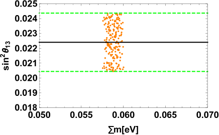
Figure 1: The sum of neutrino masses $\sum m(\equiv$ Tr$[D_{\nu}]$) versus $\sin^{2}\theta_{12}$(red color), $\sin^{2}\theta_{23}$(blue color) in the left figure, and $\sin^{2}\theta_{13}$(orange color) in the right figure. Here, the horizontal black solid lines are the best fit values, the green dotted lines show 3$\sigma$ range, and the vertical black line shows upper bound on the cosmological data as shown in the neutrino section.

Figure 1 shows the sum of neutrino masses $\sum m(\equiv$ Tr$[D_{\nu}])$ versus $\sin^{2}\theta_{12}$(red color), $\sin^{2}\theta_{23}$(blue color) in the left figure, and $\sin^{2}\theta_{13}$ in the right figure. Here, the horizontal black solid lines are the best fit values, the green dotted lines show 3$\sigma$ range, and the vertical black line shows upper bound on the cosmological data as shown in the neutrino section. It suggests that all the three mixings run over whole the range of experimental results at 3$\sigma$ interval, even though larger value of $\sin^{2}\theta_{23}$ is somewhat favored. While the sum of neutrino masses is restricted to be $\sum m\approx$0.06 eV that always satisfies the upper bound on the cosmological result.

Figure 2: Phase of $\delta^{\ell}_{CP}$ in terms of $\alpha_{31}$.

Figure 2 shows phase of $\delta^{\ell}_{CP}$ in terms of $\alpha_{31}$. This figure implies that Dirac CP is linearly proportional to $\alpha_{31}$ phase that runs over whole the ranges. Once the Dirac CP phase could be fixed to be $\sim 270$ [deg] in future experiments, $\alpha_{31}$ is predicted to be $\sim$ 200 [deg].

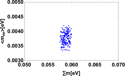
Figure 3: The sum of neutrino masses versus the effective mass for the neutrinoless double beta decay.

Figure 3 demonstrates the sum of neutrino masses versus the effective mass for the neutrinoless double beta decay. It suggests that 0.0035 eV $\lesssim\langle m_{ee}\rangle\lesssim$ 0.045 eV. Another remarks are in order:

1. The typical region of modulus $\tau$ is found in narrow space as -0.1 $\lesssim\$Re$[\tau]\lesssim$ 0.1 and 1.2 $\lesssim\$Im$[\tau]\lesssim$ 1.3.

2. Typical scale of LFVs are very small in our analyses, therefore following upper bounds are realized:

   $${\rm BR}(\mu\to e\gamma)\lesssim 3.0\times 10^{-19},\quad{\rm BR}(\tau\to e\gamma)\lesssim 2.5\times 10^{-19},\quad{\rm BR}(\tau\to\mu\gamma)\lesssim 1.5\times 10^{-20}.$$

3. The lightest Majorana mass eigenstate is given by [2$-$9] TeV.

IV Conclusion and discussion

We have constructed a predictive lepton model with modular $S_{3}$ symmetry in framework of one-loop induced radiative seesaw model. The DM stability is naturally assured by $Z_{2}$ symmetry, and DM is correlated with neutrinos in a specific manner, where their interactions are determined by the $S_{3}$ symmetry that is known as the minimal group in non-Abelian discrete flavor symmetries. In our numerical analyses, we have highlighted several remarks as follows:

1. The Dirac phase and the Majorana phase are strongly correlated.

2. The typical region of modulus $\tau$ is found in narrow space as -0.1 $\lesssim\$Re$[\tau]\lesssim$ 0.1 and 1.2 $\lesssim\$Im$[\tau]\lesssim$ 1.3.

3. Typical scale of LFVs are very small in our analyses, therefore following upper bounds are realized:

   $${\rm BR}(\mu\to e\gamma)\lesssim 3.0\times 10^{-19},\quad{\rm BR}(\tau\to e\gamma)\lesssim 2.5\times 10^{-19},\quad{\rm BR}(\tau\to\mu\gamma)\lesssim 1.5\times 10^{-20}.$$

4. The lightest Majorana mass eigenstate is given by [2$-$9] TeV.

References

• (1) E. Ma, Phys. Rev. D 73, 077301 (2006) doi:10.1103/PhysRevD.73.077301 [hep-ph/0601225].
• (2) R. de Adelhart Toorop, F. Feruglio and C. Hagedorn, Nucl. Phys. B 858, 437 (2012) [arXiv:1112.1340 [hep-ph]].
• (3) F. Feruglio, doi:10.1142/9789813238053_0012 arXiv:1706.08749 [hep-ph].
• (4) J. C. Criado and F. Feruglio, arXiv:1807.01125 [hep-ph].
• (5) T. Kobayashi, N. Omoto, Y. Shimizu, K. Takagi, M. Tanimoto and T. H. Tatsuishi, JHEP 1811, 196 (2018) doi:10.1007/JHEP11(2018)196 [arXiv:1808.03012 [hep-ph]].
• (6) H. Okada and M. Tanimoto, Phys. Lett. B 791, 54 (2019) doi:10.1016/j.physletb.2019.02.028 [arXiv:1812.09677 [hep-ph]].
• (7) T. Nomura and H. Okada, arXiv:1904.03937 [hep-ph].
• (8) H. Okada and M. Tanimoto, arXiv:1905.13421 [hep-ph].
• (9) F. J. de Anda, S. F. King and E. Perdomo, arXiv:1812.05620 [hep-ph].
• (10) P. P. Novichkov, S. T. Petcov and M. Tanimoto, arXiv:1812.11289 [hep-ph].
• (11) T. Nomura and H. Okada, arXiv:1906.03927 [hep-ph].
• (12) G. J. Ding, S. F. King and X. G. Liu, arXiv:1907.11714 [hep-ph].
• (13) H. Okada and Y. Orikasa, arXiv:1907.13520 [hep-ph].
• (14) T. Nomura, H. Okada and O. Popov, arXiv:1908.07457 [hep-ph].
• (15) T. Kobayashi, Y. Shimizu, K. Takagi, M. Tanimoto and T. H. Tatsuishi, arXiv:1909.05139 [hep-ph].
• (16) T. Asaka, Y. Heo, T. H. Tatsuishi and T. Yoshida, arXiv:1909.06520 [hep-ph].
• (17) G. J. Ding, S. F. King, X. G. Liu and J. N. Lu, arXiv:1910.03460 [hep-ph].
• (18) D. Zhang, arXiv:1910.07869 [hep-ph].
• (19) T. Kobayashi, K. Tanaka and T. H. Tatsuishi, Phys. Rev. D 98 (2018) no.1, 016004 [arXiv:1803.10391 [hep-ph]].
• (20) T. Kobayashi, Y. Shimizu, K. Takagi, M. Tanimoto, T. H. Tatsuishi and H. Uchida, Phys. Lett. B 794, 114 (2019) doi:10.1016/j.physletb.2019.05.034 [arXiv:1812.11072 [hep-ph]].
• (21) T. Kobayashi, Y. Shimizu, K. Takagi, M. Tanimoto and T. H. Tatsuishi, arXiv:1906.10341 [hep-ph].
• (22) J. T. Penedo and S. T. Petcov, Nucl. Phys. B 939, 292 (2019) doi:10.1016/j.nuclphysb.2018.12.016 [arXiv:1806.11040 [hep-ph]].
• (23) P. P. Novichkov, J. T. Penedo, S. T. Petcov and A. V. Titov, JHEP 1904, 005 (2019) doi:10.1007/JHEP04(2019)005 [arXiv:1811.04933 [hep-ph]].
• (24) T. Kobayashi, Y. Shimizu, K. Takagi, M. Tanimoto and T. H. Tatsuishi, arXiv:1907.09141 [hep-ph].
• (25) S. F. King and Y. L. Zhou, arXiv:1908.02770 [hep-ph].
• (26) H. Okada and Y. Orikasa, arXiv:1908.08409 [hep-ph].
• (27) J. C. Criado, F. Feruglio, F. Feruglio and S. J. D. King, arXiv:1908.11867 [hep-ph].
• (28) X. Wang and S. Zhou, arXiv:1910.09473 [hep-ph].
• (29) P. P. Novichkov, J. T. Penedo, S. T. Petcov and A. V. Titov, arXiv:1812.02158 [hep-ph].
• (30) G. J. Ding, S. F. King and X. G. Liu, arXiv:1903.12588 [hep-ph].
• (31) A. Baur, H. P. Nilles, A. Trautner and P. K. S. Vaudrevange, arXiv:1901.03251 [hep-th].
• (32) I. de Medeiros Varzielas, S. F. King and Y. L. Zhou, arXiv:1906.02208 [hep-ph]. citeLiu:2019khw
• (33) X. G. Liu and G. J. Ding, arXiv:1907.01488 [hep-ph].
• (34) G. Altarelli and F. Feruglio, Rev. Mod. Phys.  82 (2010) 2701 [arXiv:1002.0211 [hep-ph]].
• (35) H. Ishimori, T. Kobayashi, H. Ohki, Y. Shimizu, H. Okada and M. Tanimoto, Prog. Theor. Phys. Suppl.  183 (2010) 1 [arXiv:1003.3552 [hep-th]].
• (36) H. Ishimori, T. Kobayashi, H. Ohki, H. Okada, Y. Shimizu and M. Tanimoto, Lect. Notes Phys.  858 (2012) 1, Springer.
• (37) D. Hernandez and A. Y. Smirnov, Phys. Rev. D 86 (2012) 053014 [arXiv:1204.0445 [hep-ph]].
• (38) S. F. King and C. Luhn, Rept. Prog. Phys.  76 (2013) 056201 [arXiv:1301.1340 [hep-ph]].
• (39) S. F. King, A. Merle, S. Morisi, Y. Shimizu and M. Tanimoto, arXiv:1402.4271 [hep-ph].
• (40) S. F. King, Prog. Part. Nucl. Phys.  94 (2017) 217 doi:10.1016/j.ppnp.2017.01.003 [arXiv:1701.04413 [hep-ph]].
• (41) S. T. Petcov, Eur. Phys. J. C 78 (2018) no.9, 709 [arXiv:1711.10806 [hep-ph]].
• (42) Z. z. Xing, arXiv:1909.09610 [hep-ph].
• (43) A. Baur, H. P. Nilles, A. Trautner and P. K. S. Vaudrevange, Nucl. Phys. B 947, 114737 (2019) doi:10.1016/j.nuclphysb.2019.114737 [arXiv:1908.00805 [hep-th]].
• (44) T. Kobayashi, Y. Shimizu, K. Takagi, M. Tanimoto, T. H. Tatsuishi and H. Uchida, arXiv:1910.11553 [hep-ph].
• (45) M. Hirsch, S. Morisi, E. Peinado and J. W. F. Valle, Phys. Rev. D 82, 116003 (2010) doi:10.1103/PhysRevD.82.116003 [arXiv:1007.0871 [hep-ph]].
• (46) J. M. Lamprea and E. Peinado, Phys. Rev. D 94, no. 5, 055007 (2016) doi:10.1103/PhysRevD.94.055007 [arXiv:1603.02190 [hep-ph]].
• (47) L. M. G. De La Vega, R. Ferro-Hernandez and E. Peinado, Phys. Rev. D 99, no. 5, 055044 (2019) doi:10.1103/PhysRevD.99.055044 [arXiv:1811.10619 [hep-ph]].
• (48) P. P. Novichkov, J. T. Penedo, S. T. Petcov and A. V. Titov, arXiv:1905.11970 [hep-ph].
• (49) S. Baek, T. Nomura and H. Okada, Phys. Lett. B 759, 91 (2016) doi:10.1016/j.physletb.2016.05.055 [arXiv:1604.03738 [hep-ph]].
• (50) M. Lindner, M. Platscher and F. S. Queiroz, Phys. Rept.  731, 1 (2018) doi:10.1016/j.physrep.2017.12.001 [arXiv:1610.06587 [hep-ph]].
• (51) A. M. Baldini et al. [MEG Collaboration], Eur. Phys. J. C 76, no. 8, 434 (2016) [arXiv:1605.05081 [hep-ex]].
• (52) F. Renga [MEG Collaboration], Hyperfine Interact.  239, no. 1, 58 (2018) [arXiv:1811.05921 [hep-ex]].
• (53) B. Aubert et al. [BaBar Collaboration], Phys. Rev. Lett.  104 (2010) 021802 [arXiv:0908.2381 [hep-ex]].
• (54) N. Aghanim et al. [Planck Collaboration], arXiv:1807.06209 [astro-ph.CO].
• (55) A. Gando et al. [KamLAND-Zen Collaboration], Phys. Rev. Lett.  117, no. 8, 082503 (2016) Addendum: [Phys. Rev. Lett.  117, no. 10, 109903 (2016)] doi:10.1103/PhysRevLett.117.109903, 10.1103/PhysRevLett.117.082503 [arXiv:1605.02889 [hep-ex]].
• (56) T. Hambye, F.-S. Ling, L. Lopez Honorez and J. Rocher, JHEP 0907, 090 (2009) Erratum: [JHEP 1005, 066 (2010)] doi:10.1007/JHEP05(2010)066, 10.1088/1126-6708/2009/07/090 [arXiv:0903.4010 [hep-ph]].
• (57) I. Esteban, M. C. Gonzalez-Garcia, A. Hernandez-Cabezudo, M. Maltoni and T. Schwetz, JHEP 1901, 106 (2019) doi:10.1007/JHEP01(2019)106 [arXiv:1811.05487 [hep-ph]].