Supplement to Paper: Characterizing Inter-Layer Functional Mappings of Deep Learning Models

S.1 Statistical analysis using Euclidean distance as measure of proximity

This supplemental material presents more detailed results from the three experiments (CIFAR10 with random labels, CIFAR10 with true labels, and MNIST with true labels) using the Euclidean distance metric for the proximity measure of the HP statistics.

Figure S-1 shows the between-class HP statistics of the raw images, or class separability in the original measurement space. The comparisons were made using the analysis subset of the training data (1000 images per class) and the validation data (1000 images per class). As described in Section 3 of the paper, for the case using CIFAR10 with random labels there are five different versions of the randomly permuted labels; one per instance of the training network. The results for only one of these versions is tabulated and plotted in Figures S-1 (A) and (D), respectively.

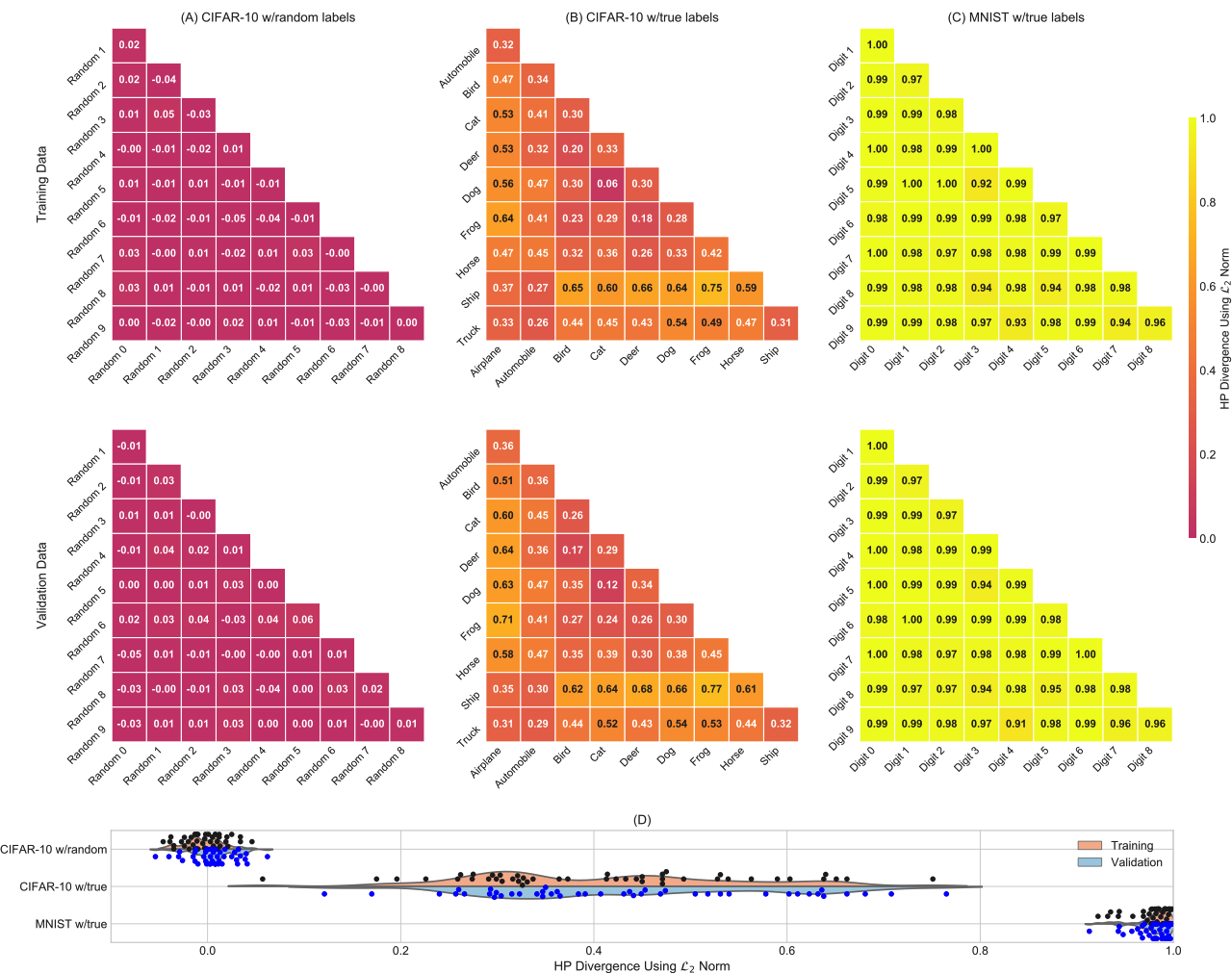
Figure S-1: Pairwise class HP statistics using Euclidean distance (training data above, validation data below) computed on (A) CIFAR10 with random labels, (B) CIFAR10 with true labels, and (C) MNIST with true labels. (D) The $\boldsymbol{\mathcal{H}}^{(t)}$ (black dots above) and $\boldsymbol{\mathcal{H}}^{(v)}$(blue dots, below) values and respective kernel-based density functions (orange = training, blue = validation) for each task which illustrate that the estimated class separation for each task in their respective ambient representations are quite distinct.

Figures S-2 through S-6 present the class-wise HP statistics of the training and validation samples of the CIFAR10 data with random labels as they pass through an associated model. Each figure plots the results for one of the five training instances discussed in Section 3 of the paper. The (a) subfigures show the data passing through the untrained models and the (b) subfigures show the data passing through the trained version of the models. Similarly, Figures S-7 through S-11 present plots for the 5 model instances trained on the CIFAR10 data with true labels, and Figures S-12 through S-16 show the plots for the 5 MNIST-trained models.

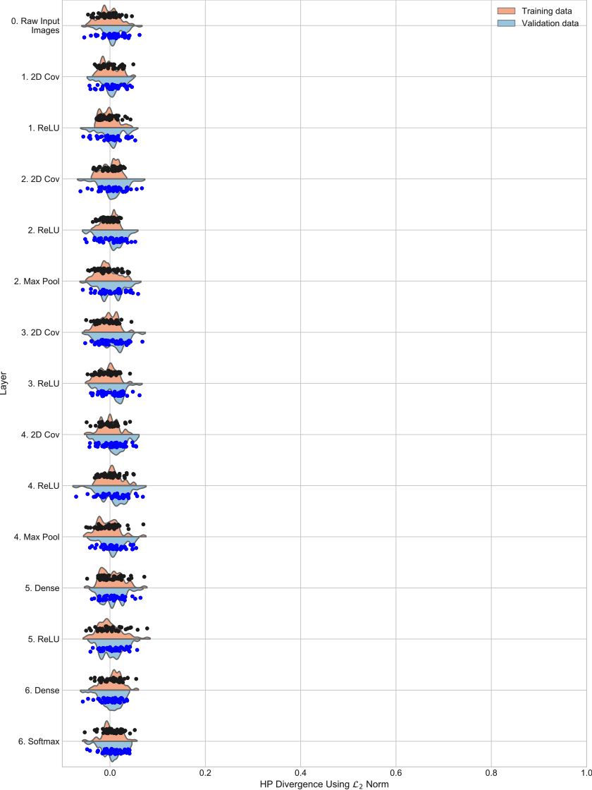
(a) Untrained model

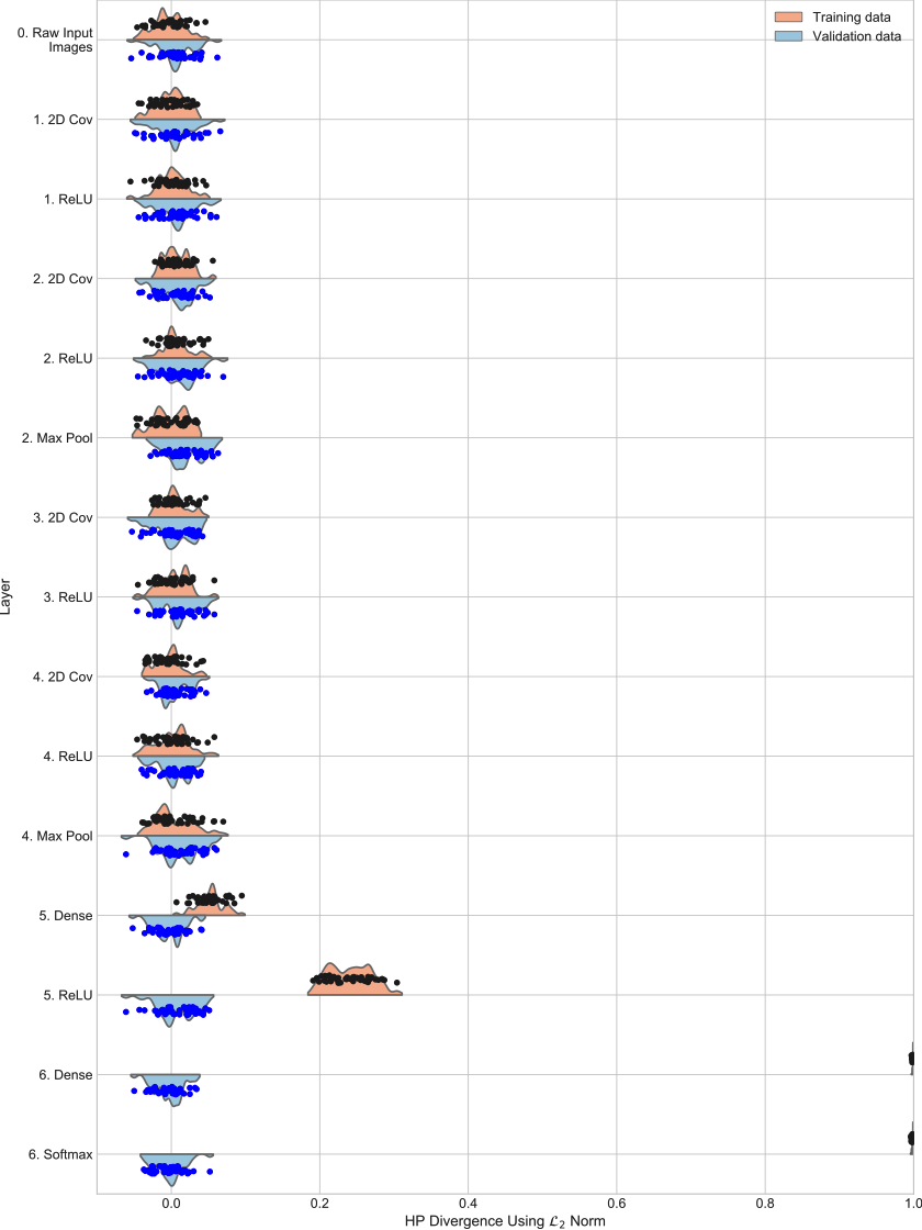
(b) Trained model

Figure S-2: $\mathcal{H}$ class-pair statistics at each layer for instance 1 of the model for CIFAR10 with random class labels. (a) shows results for the data for passing through the randomly initialized model (epoch 0 state). (b) shows the results for the data passing through the fully trained model (epoch 200 state). (Note: Euclidean distance is used as the proximity measure.)

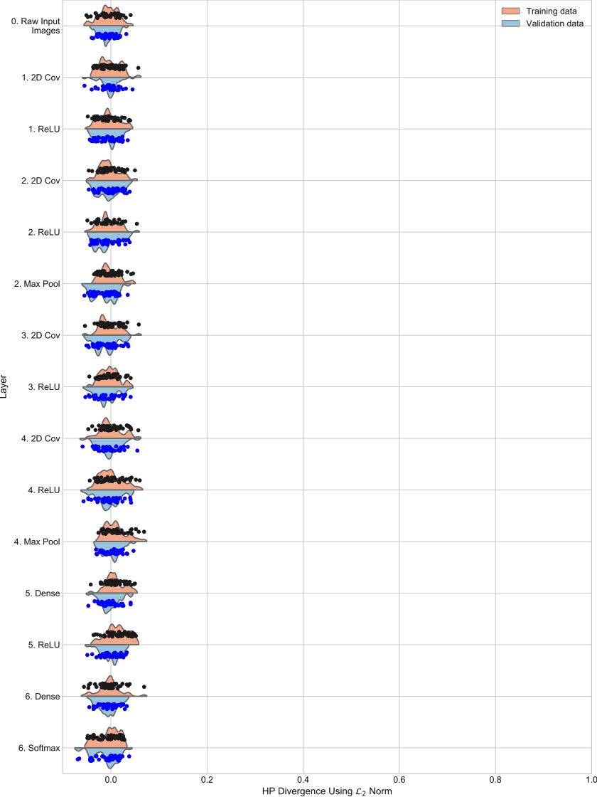
(a) Untrained model

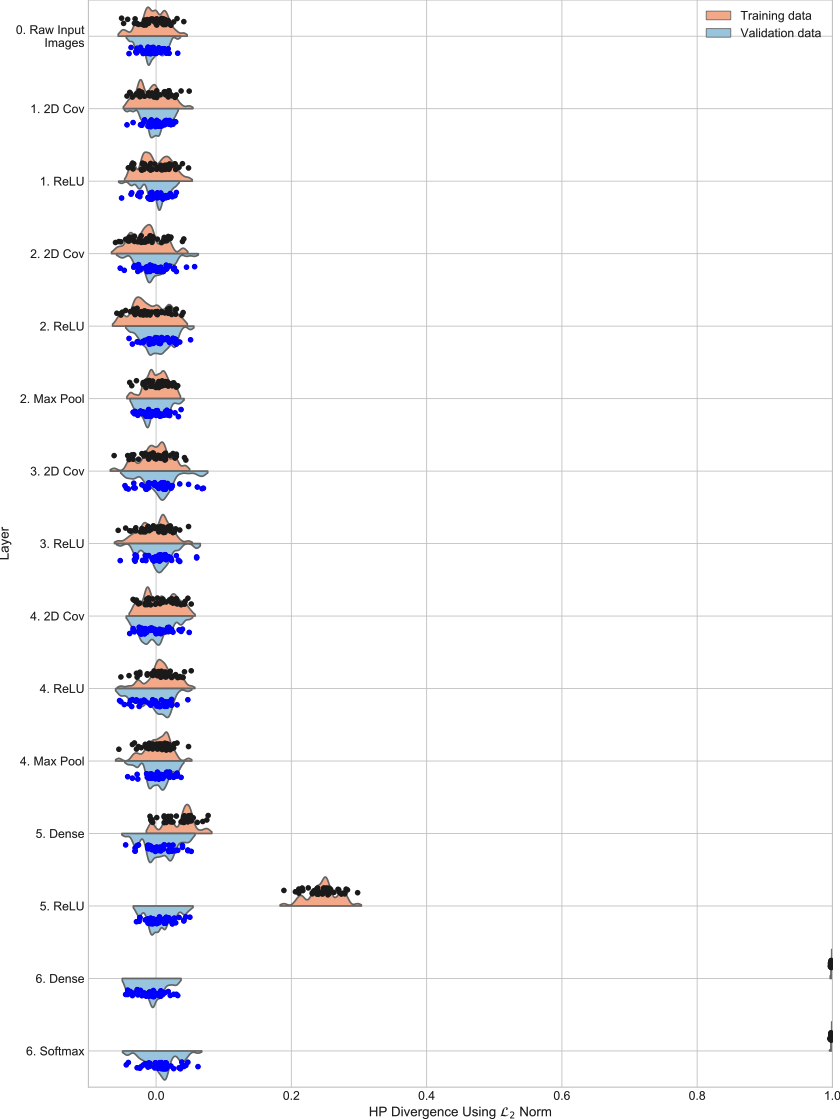
(b) Trained model

Figure S-3: $\mathcal{H}$ class-pair statistics at each layer for instance 2 of the model for CIFAR10 with random class labels. (a) shows results for the data for passing through the randomly initialized model (epoch 0 state). (b) shows the results for the data passing through the fully trained model (epoch 200 state). (Note: Euclidean distance is used as the proximity measure.)

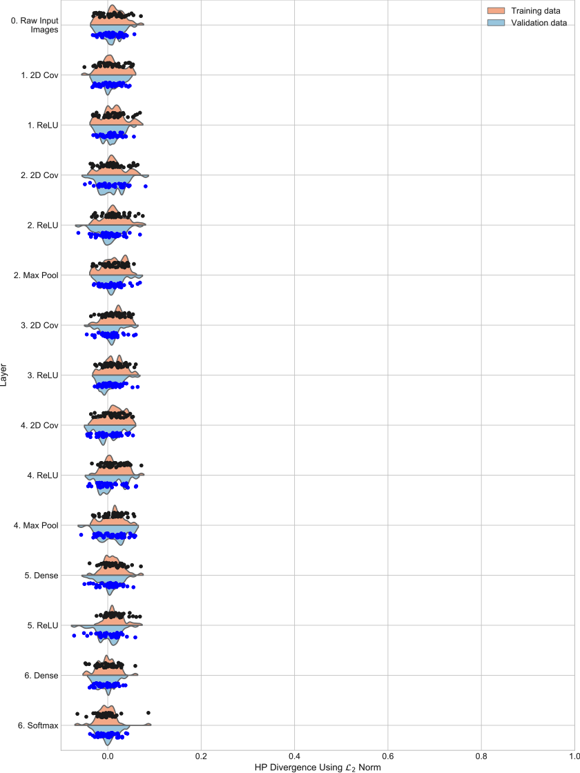
(a) Untrained model

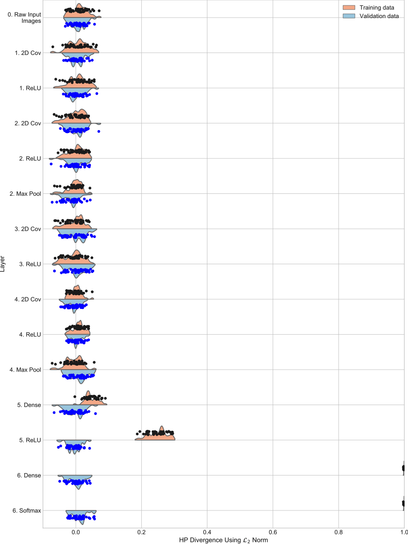
(b) Trained model

Figure S-4: $\mathcal{H}$ class-pair statistics at each layer for instance 3 of the model for CIFAR10 with random class labels. (a) shows results for the data for passing through the randomly initialized model (epoch 0 state). (b) shows the results for the data passing through the fully trained model (epoch 200 state). (Note: Euclidean distance is used as the proximity measure.)

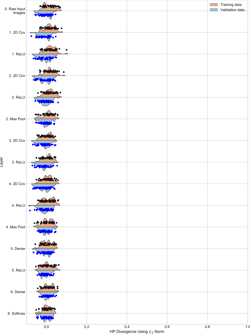
(a) Untrained model

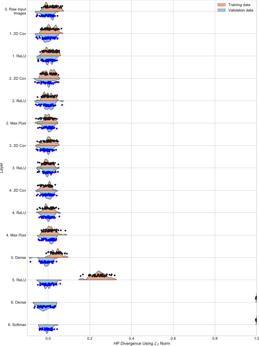
(b) Trained model

Figure S-5: $\mathcal{H}$ class-pair statistics at each layer for instance 4 of the model for CIFAR10 with random class labels. (a) shows results for the data for passing through the randomly initialized model (epoch 0 state). (b) shows the results for the data passing through the fully trained model (epoch 200 state). (Note: Euclidean distance is used as the proximity measure.)

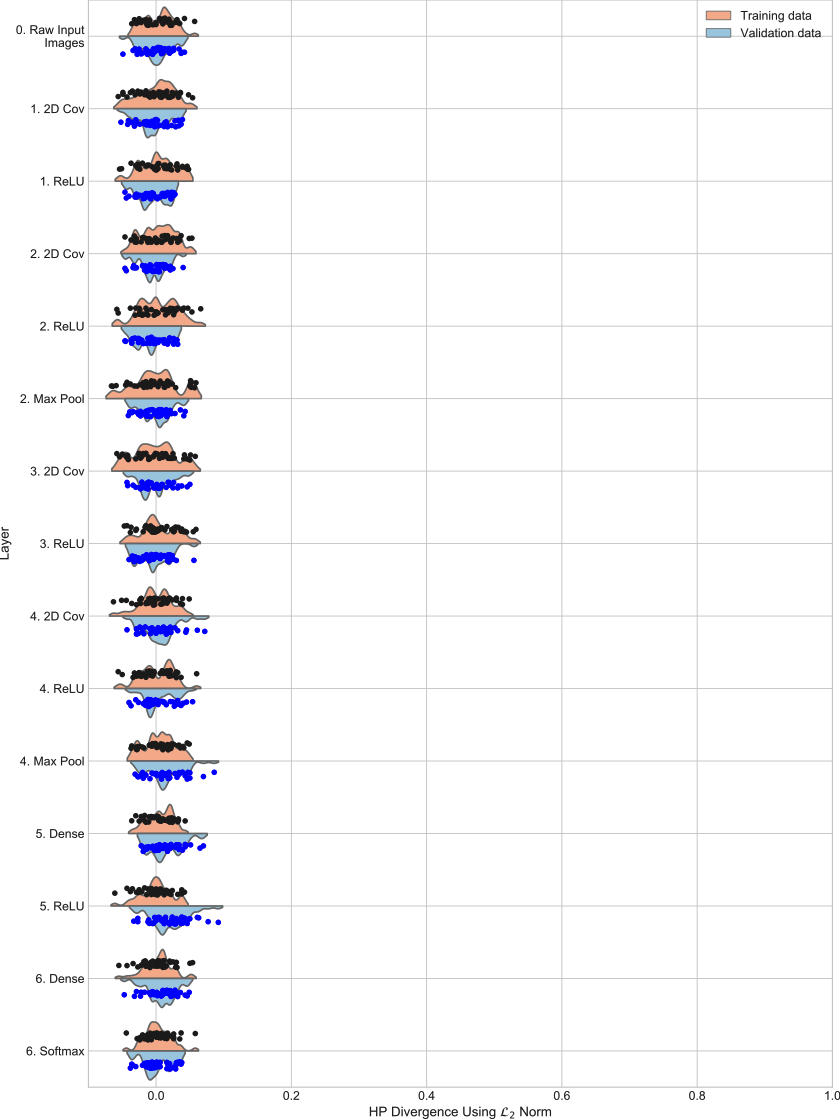
(a) Untrained model

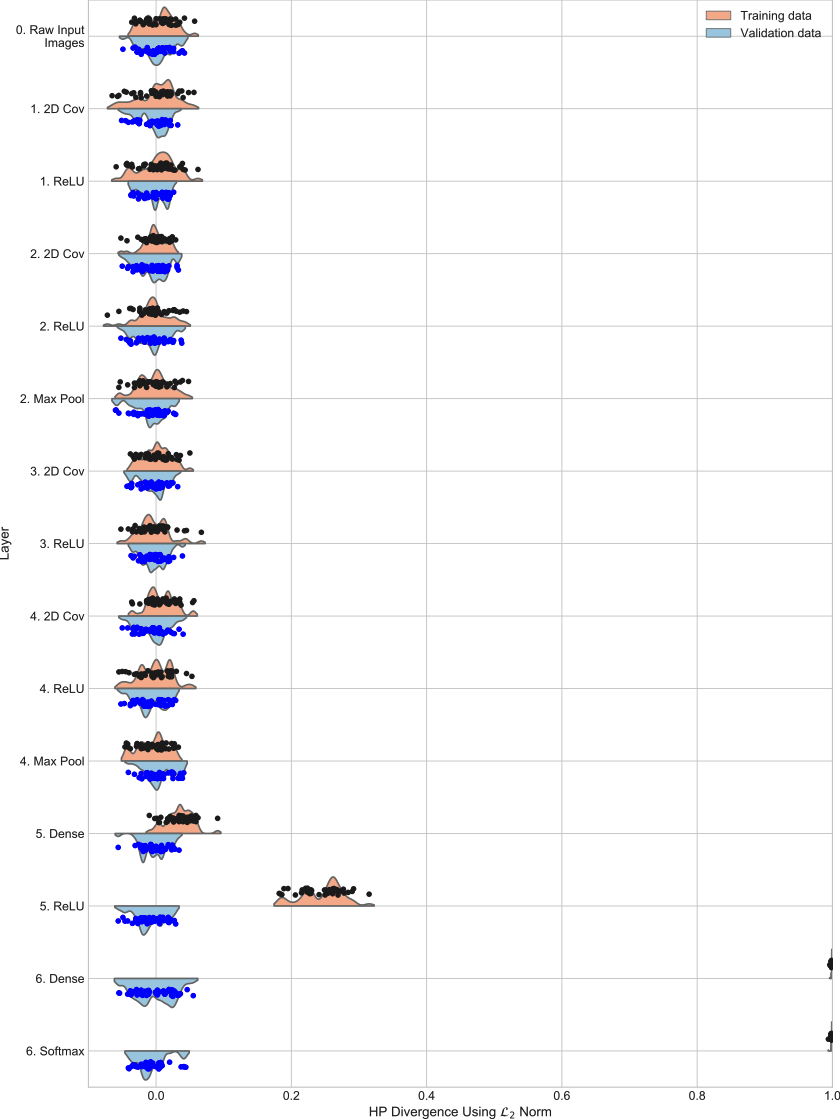
(b) Trained model

Figure S-6: $\mathcal{H}$ class-pair statistics at each layer for instance 5 of the model for CIFAR10 with random class labels. (a) shows results for the data for passing through the randomly initialized model (epoch 0 state). (b) shows the results for the data passing through the fully trained model (epoch 200 state). (Note: Euclidean distance is used as the proximity measure.)

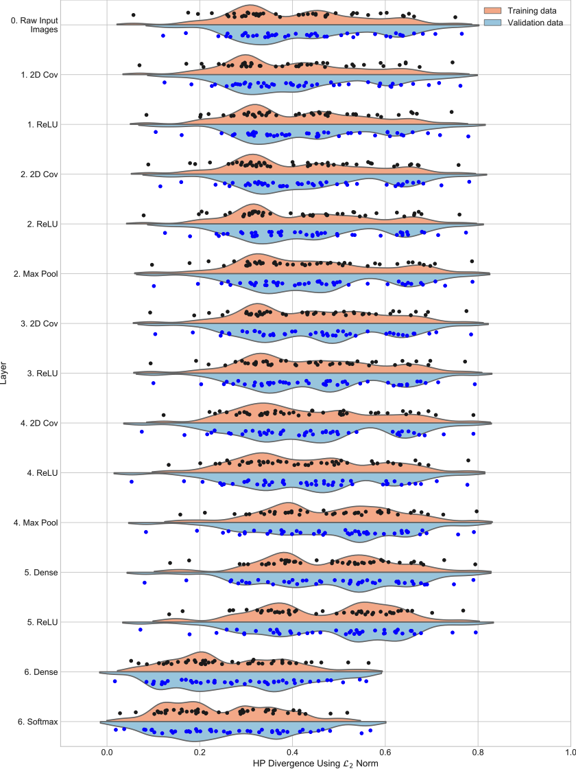
(a) Untrained model

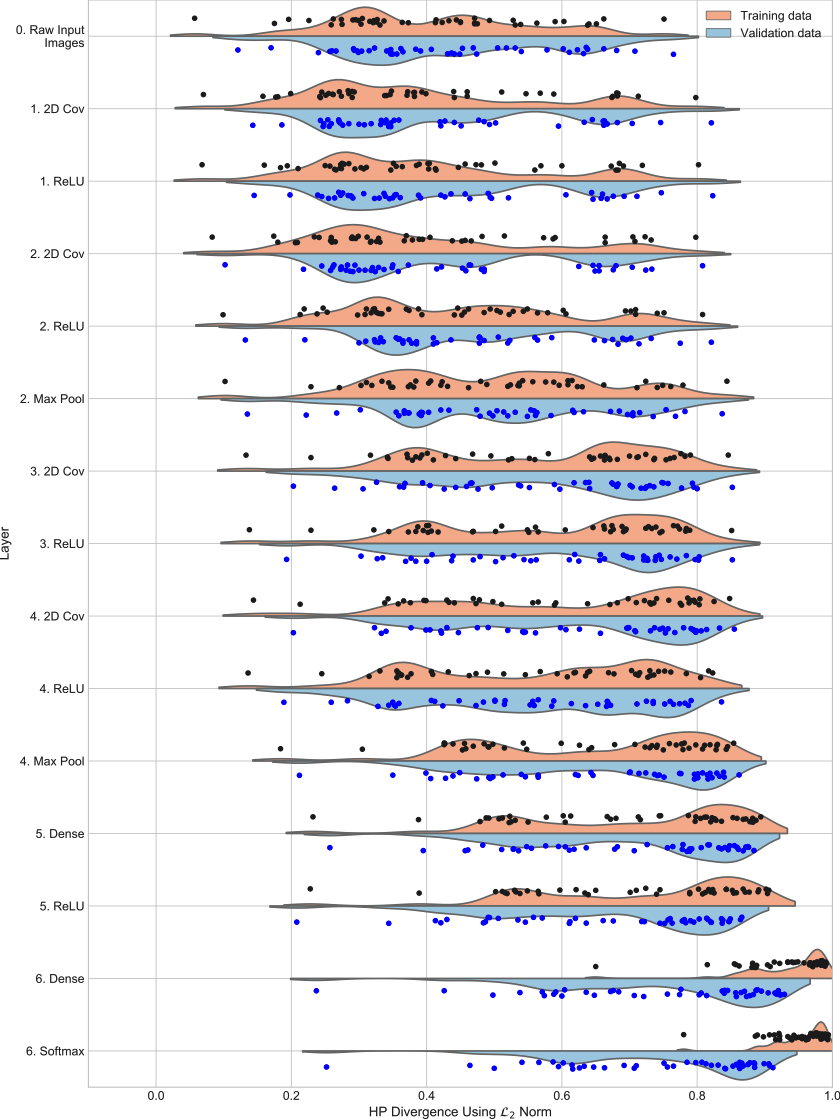
(b) Trained model

Figure S-7: $\mathcal{H}$ class-pair statistics at each layer for instance 1 of the model for CIFAR10 with true class labels. (a) shows results for the data for passing through the randomly initialized model (epoch 0 state). (b) shows the results for the data passing through the fully trained model (stopping at peak validation set accuracy). (Note: Euclidean distance is used as the proximity measure.)

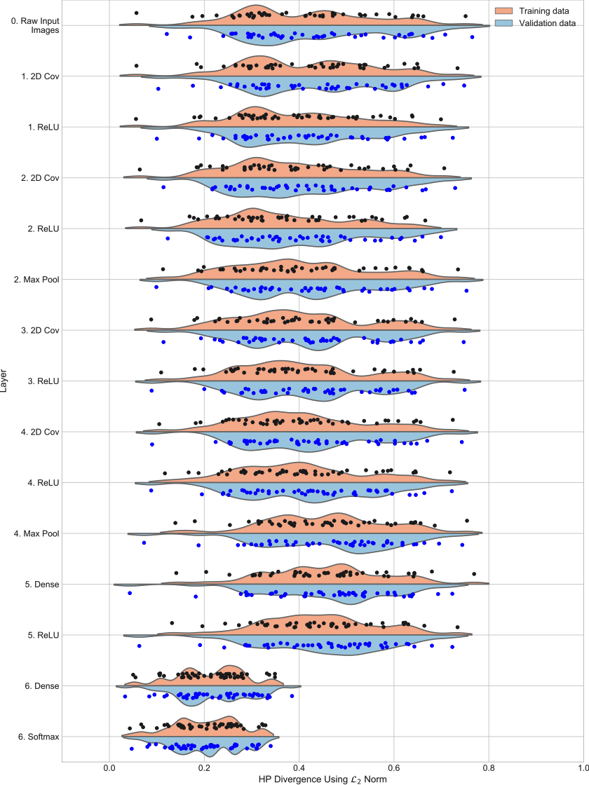
(a) Untrained model

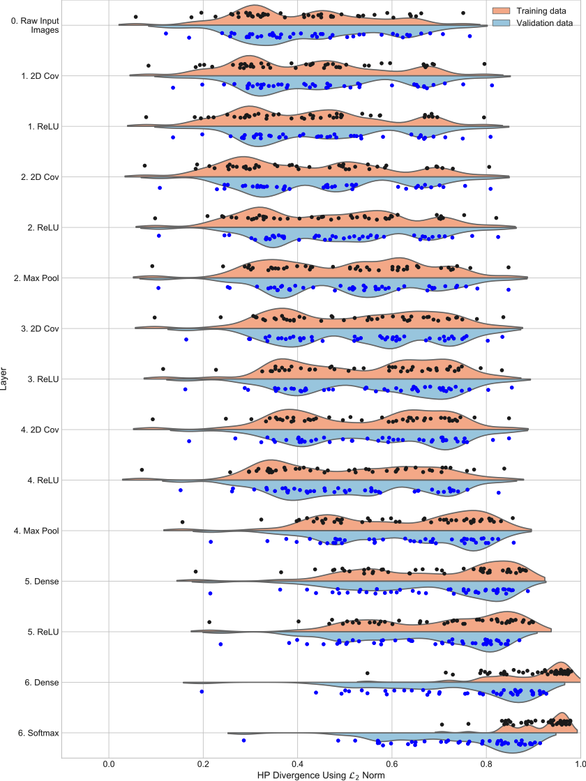
(b) Trained model

Figure S-8: $\mathcal{H}$ class-pair statistics at each layer for instance 2 of the model for CIFAR10 with true class labels. (a) shows results for the data for passing through the randomly initialized model (epoch 0 state). (b) shows the results for the data passing through the fully trained model (stopping at peak validation set accuracy). (Note: Euclidean distance is used as the proximity measure.)

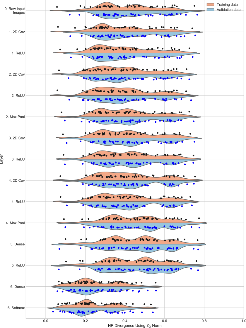
(a) Untrained model

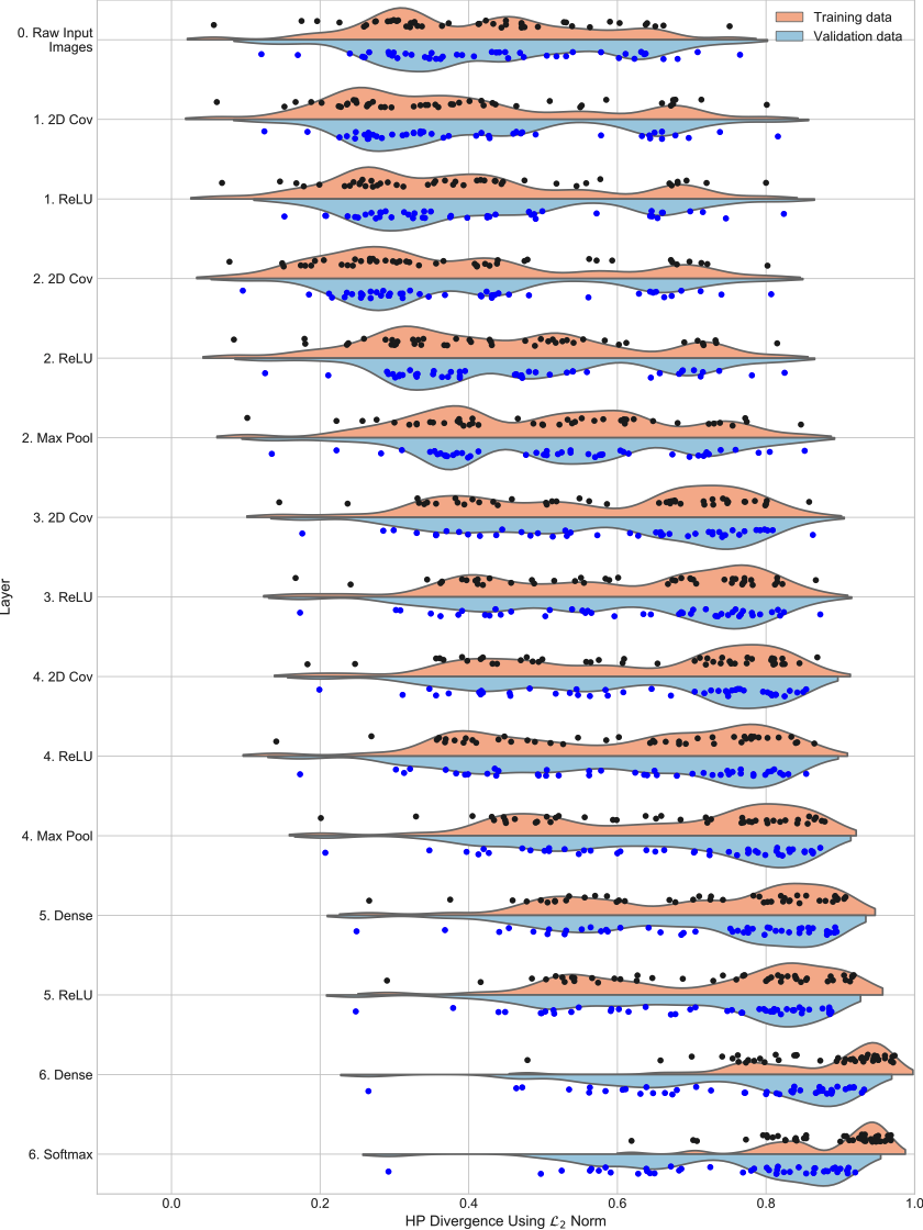
(b) Trained model

Figure S-9: $\mathcal{H}$ class-pair statistics at each layer for instance 3 of the model for CIFAR10 with true class labels. (a) shows results for the data for passing through the randomly initialized model (epoch 0 state). (b) shows the results for the data passing through the fully trained model (stopping at peak validation set accuracy). (Note: Euclidean distance is used as the proximity measure.)

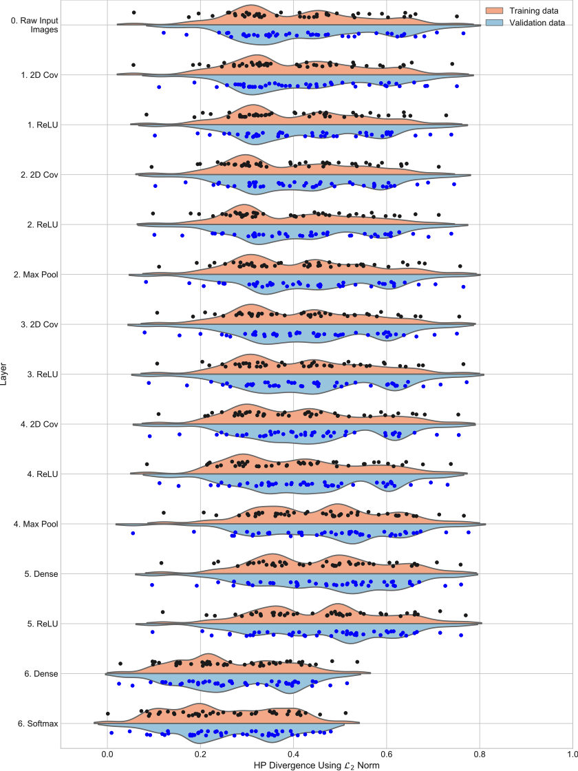
(a) Untrained model

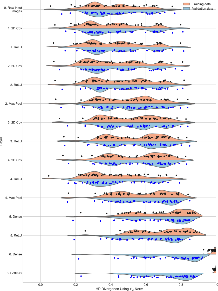
(b) Trained model

Figure S-10: $\mathcal{H}$ class-pair statistics at each layer for instance 4 of the model for CIFAR10 with true class labels. (a) shows results for the data for passing through the randomly initialized model (epoch 0 state). (b) shows the results for the data passing through the fully trained model (stopping at peak validation set accuracy). (Note: Euclidean distance is used as the proximity measure.)

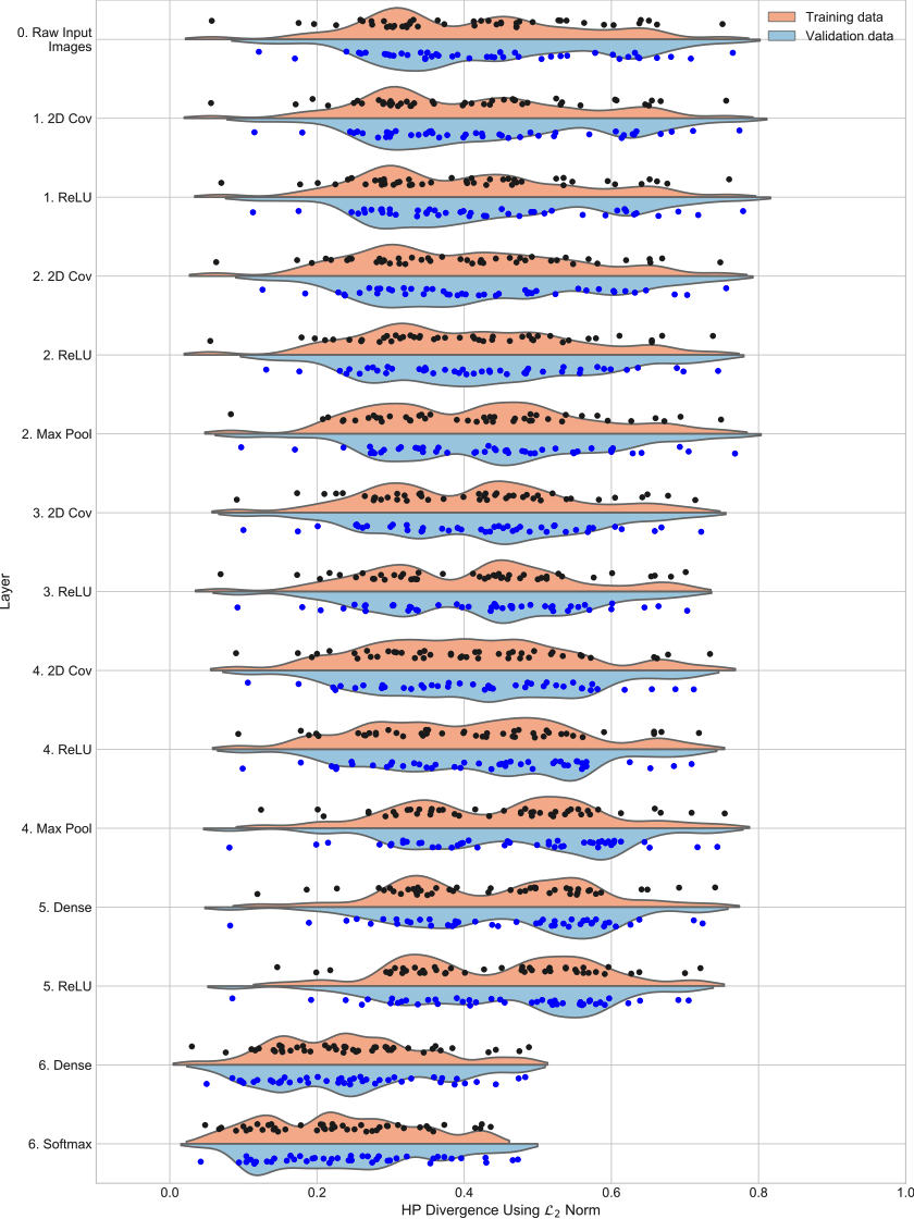
(a) Untrained model

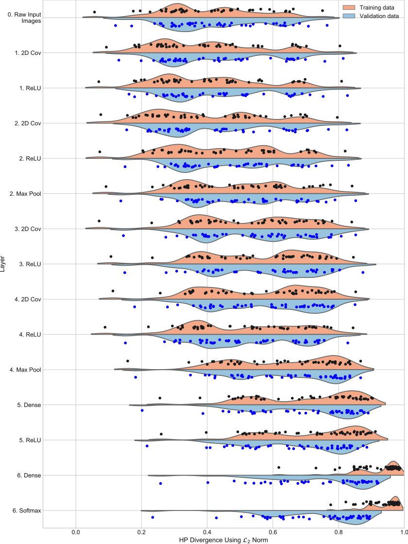
(b) Trained model

Figure S-11: $\mathcal{H}$ class-pair statistics at each layer for instance 5 of the model for CIFAR10 with true class labels. (a) shows results for the data for passing through the randomly initialized model (epoch 0 state). (b) shows the results for the data passing through the fully trained model (stopping at peak validation set accuracy). (Note: Euclidean distance is used as the proximity measure.)

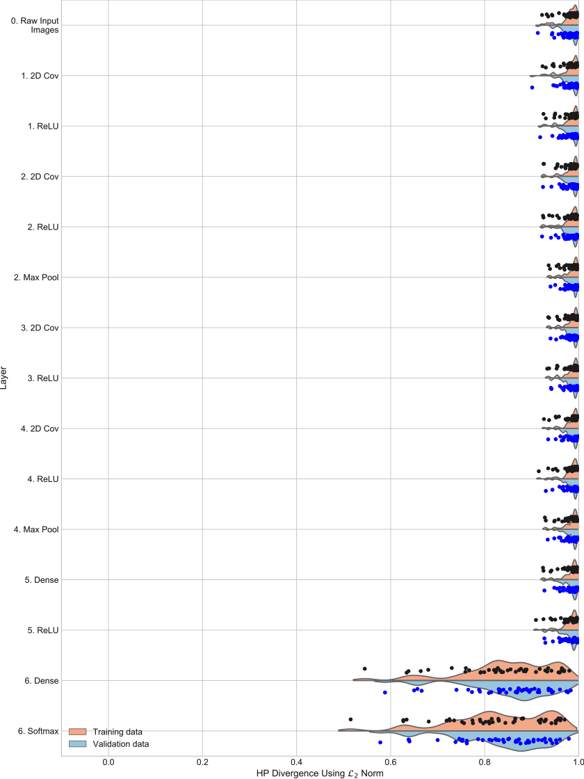
(a) Untrained model

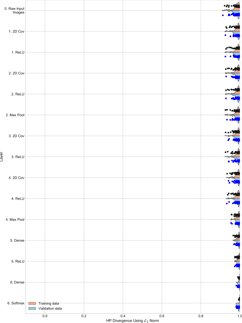
(b) Trained model

Figure S-12: $\mathcal{H}$ class-pair statistics at each layer for instance 1 of the model for MNIST with true class labels. (a) shows results for the data for passing through the randomly initialized model (epoch 0 state). (b) shows the results for the data passing through the fully trained model (stopping at peak validation set accuracy). (Note: Euclidean distance is used as the proximity measure.)

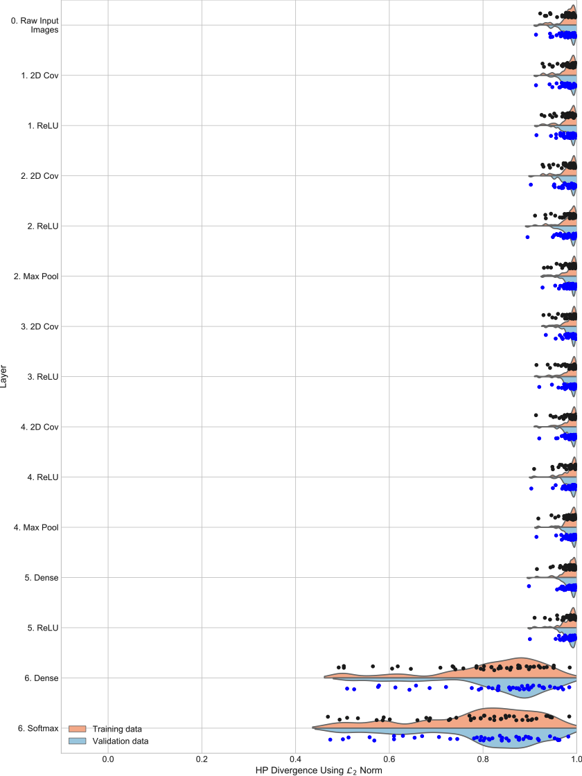
(a) Untrained model

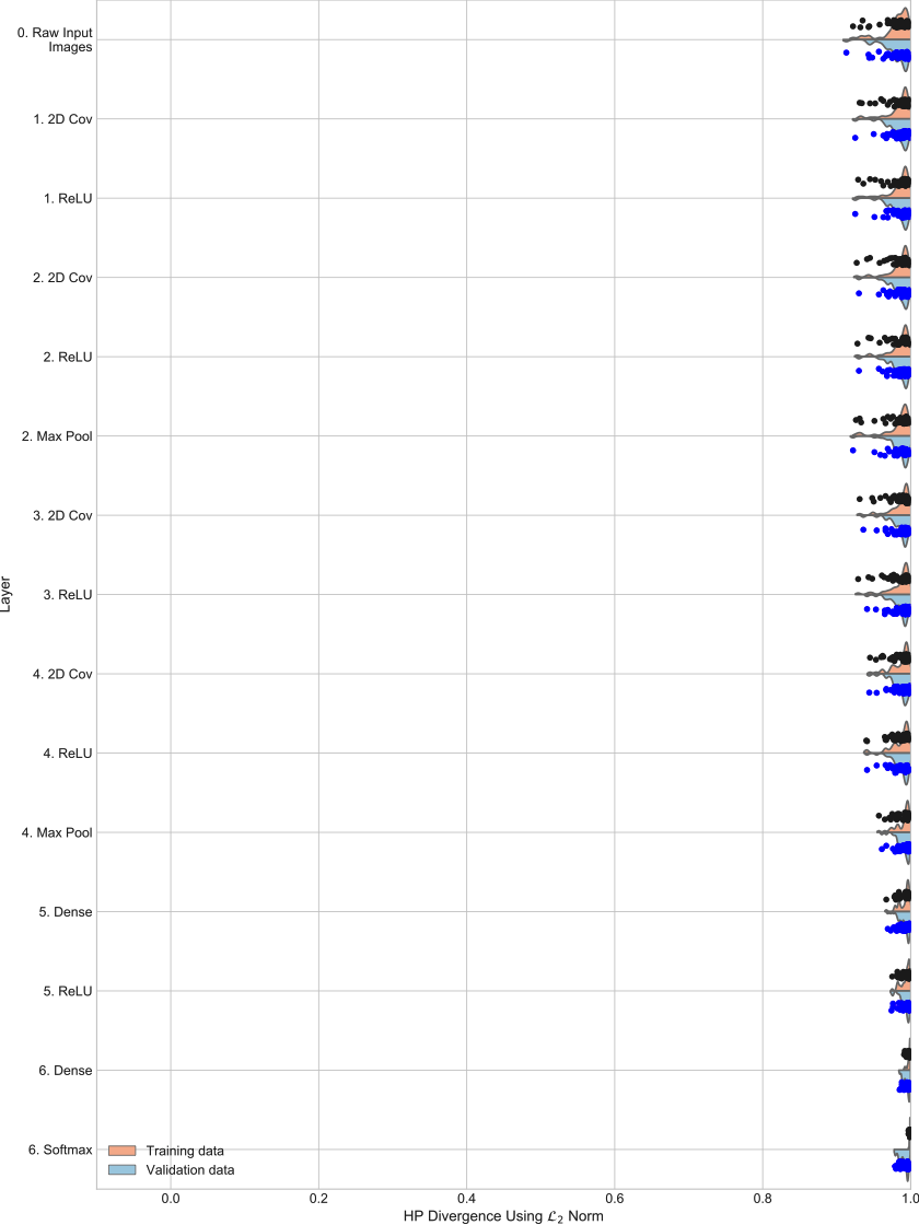
(b) Trained model

Figure S-13: $\mathcal{H}$ class-pair statistics at each layer for instance 2 of the model for MNIST with true class labels. (a) shows results for the data for passing through the randomly initialized model (epoch 0 state). (b) shows the results for the data passing through the fully trained model (stopping at peak validation set accuracy). (Note: Euclidean distance is used as the proximity measure.)

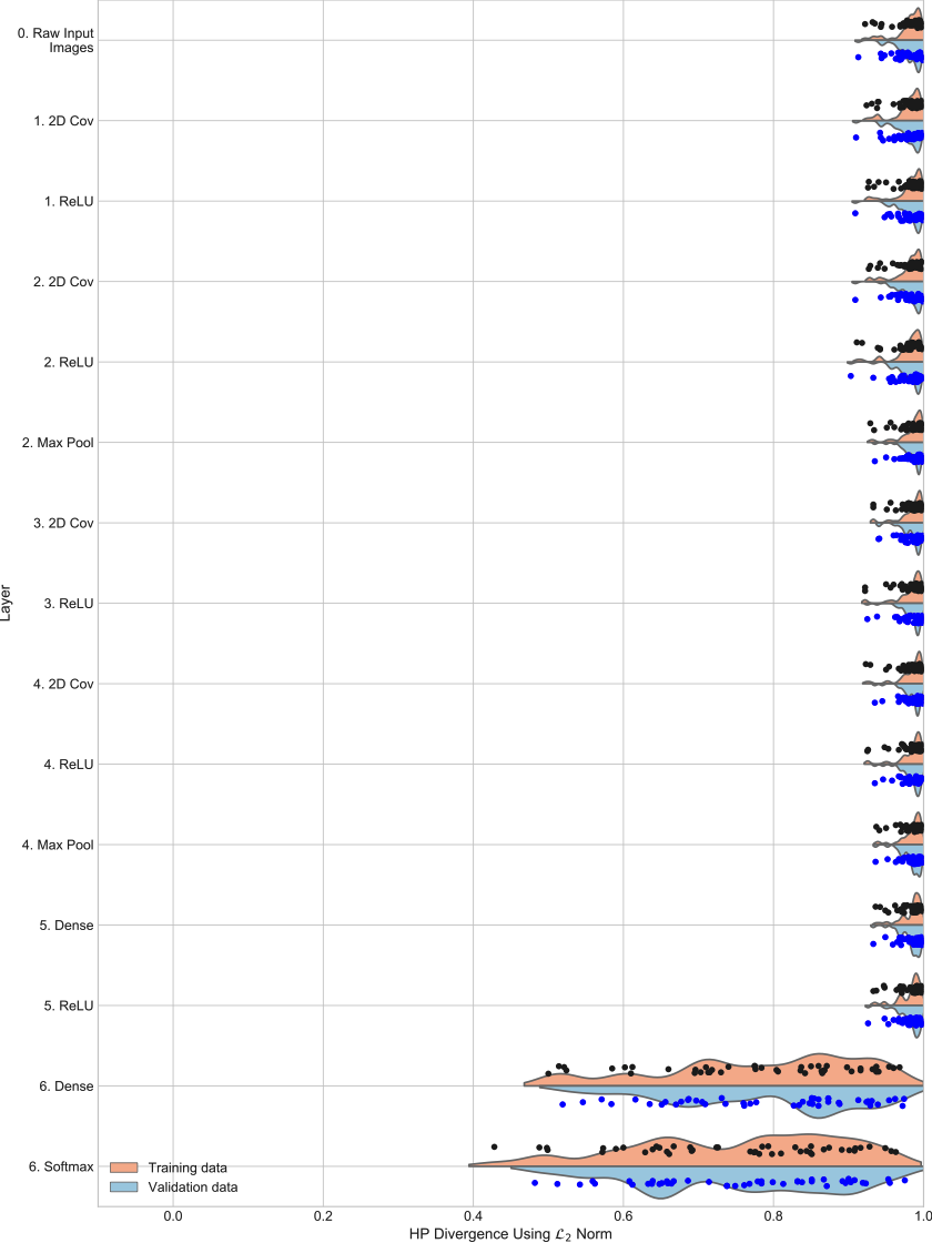
(a) Untrained model

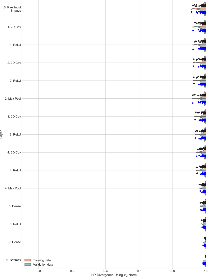
(b) Trained model

Figure S-14: $\mathcal{H}$ class-pair statistics at each layer for instance 3 of the model for MNIST with true class labels. (a) shows results for the data for passing through the randomly initialized model (epoch 0 state). (b) shows the results for the data passing through the fully trained model (stopping at peak validation set accuracy). (Note: Euclidean distance is used as the proximity measure.)

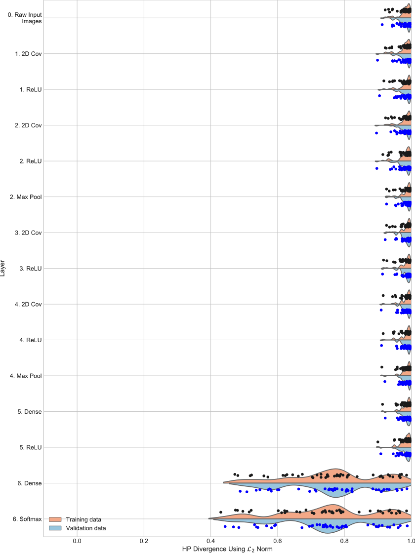
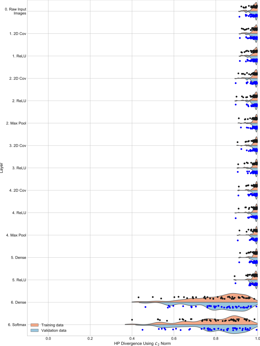
(a) Untrained model

(b) Trained model

Figure S-15: $\mathcal{H}$ class-pair statistics at each layer for instance 4 of the model for MNIST with true class labels. (a) shows results for the data for passing through the randomly initialized model (epoch 0 state). (b) shows the results for the data passing through the fully trained model (stopping at peak validation set accuracy). (Note: Euclidean distance is used as the proximity measure.)

(a) Untrained model

(b) Trained model

Figure S-16: $\mathcal{H}$ class-pair statistics at each layer for instance 5 of the model for MNIST with true class labels. (a) shows results for the data for passing through the randomly initialized model (epoch 0 state). (b) shows the results for the data passing through the fully trained model (stopping at peak validation set accuracy). (Note: Euclidean distance is used as the proximity measure.)

Tables S-1 through S-9 present a superset of the results of two-sample null hypothesis tests of means presented in the main body of the paper. In particular Tables S-4, S-5, S-7, and S-8 show the test performed between multi-layer components of the networks. The tables flag cases where the estimated $p$-values are $<0.025$. Note that the tests were performed using the random permutation algorithm with 50,000 Monte Carlo trials.

Table S-1: Two-sided permutation test of training data to detect change in $\bar{\mathcal{H}}$ between layers (before training) with critical value $\alpha=0.025$. Red font denote layer instances for which we reject $\mathbf{H_{0}}$, black font denotes layers for which we fail to reject $\mathbf{H_{0}}$. (Eq. 14 in paper) (Note: Euclidean distance is used as the proximity measure. 50,000 Monte Carlo trials were used to estimate the $p$-values. $\Delta{\bar{\mathcal{H}}}=\bar{\mathcal{H}}^{(t)}_{(k,0)}-\bar{\mathcal{H}}^{(t)}_{(k-1,0)}$))

Input Space	Output Space	CIFAR10 w Random		CIFAR10 w True		MNIST w True
		$\Delta{\bar{\mathcal{H}}}$	p-values	$\Delta{\bar{\mathcal{H}}}$	p-values	$\Delta{\bar{\mathcal{H}}}$	p-values
0.Input	1.Conv	.003; .002; -.004; .003; -.003	.460; .649; .445; .556; .515	-.012; .005; -.017; -.003; -.004	.714; .864; .593; .923; .912	.002; .001; -.001; .000; .000	.672; .792; .864; .934; .900
1.Conv	1.ReLU	-.002; -.003; .004; .002; .003	.531; .523; .434; .675; .641	.016; -.022; -.003; .001; -.000	.607; .463; .933; .969; .991	.001; .000; .001; .002; .000	.875; .906; .713; .648; .918
1.ReLU	2.Conv	.003; .001; -.001; -.002; -.001	.375; .801; .856; .650; .906	.003; -.006; -.001; -.009; -.005	.924; .842; .964; .771; .878	.000; -.000; -.001; -.001; -.000	.970; .981; .878; .826; .933
2.Conv	2.ReLU	-.001; -.002; .003; -.002; .001	.671; .626; .526; .667; .906	.002; -.017; .005; -.003; .003	.959; .562; .869; .929; .912	-.001; -.000; -.001; -.001; .001	.730; .962; .803; .748; .839
2.ReLU	2.MaxPool	-.005; .004; -.001; -.007; -.004	.202; .390; .832; .195; .576	.019; .035; .015; .020; .015	.563; .241; .623; .505; .624	.003; .003; .005; .004; .002	.365; .394; .202; .294; .565
2.MaxPool	3.Conv	.001; -.001; .004; -.006; -.003	.873; .876; .428; .286; .695	.003; -.001; .003; -.002; -.009	.936; .978; .931; .948; .755	.000; .000; -.000; -.000; .000	.998; 1.000; .998; .956; .973
3.Conv	3.ReLU	-.001; -.000; -.003; .002; .007	.747; .969; .574; .629; .246	.002; .003; .007; .004; -.002	.960; .914; .827; .895; .957	-.001; -.001; -.001; -.001; -.001	.872; .849; .721; .768; .895
3.ReLU	4.Conv	.005; .004; -.000; .000; -.005	.231; .345; .932; .954; .379	-.006; -.001; -.001; -.004; -.004	.861; .967; .975; .897; .904	.000; .001; .001; .001; .001	.998; .860; .823; .777; .842
4.Conv	4.ReLU	.005; -.000; .001; .003; .001	.220; .945; .842; .551; .821	-.003; -.003; -.006; -.008; .005	.936; .913; .851; .797; .878	-.001; .000; -.000; -.000; .000	.750; .945; .954; .893; .983
4.ReLU	4.MaxPool	-.009; .008; -.004; -.004; .004	.059; .092; .364; .425; .444	.049; .054; .040; .051; .038	.113; .061; .204; .096; .212	-.000; .000; .001; .001; .001	.962; .987; .840; .778; .777
4.MaxPool	5.Dense	.009; .000; .000; .000; .001	.061; .976; .925; .996; .838	-.005; -.001; .002; .003; -.003	.858; .976; .962; .920; .908	-.001; -.001; -.001; -.001; -.001	.758; .746; .633; .880; .682
5.Dense	5.ReLU	-.004; .004; .005; .001; -.006	.424; .385; .283; .925; .199	-.007; -.014; -.008; -.003; .003	.813; .596; .789; .908; .915	-.002; -.002; -.001; -.002; -.002	.696; .654; .723; .549; .666
5.ReLU	6.Dense	.005; -.017; -.017; .005; .003	.330; .001; .000; .305; .549	-.202; -.226; -.182; -.189; -.198	.000; .000; .000; .000; .000	-.135; -.173; -.202; -.219; -.177	.000; .000; .000; .000; .000
6.Dense	6.Softmax	-.001; -.002; -.002; -.007; -.000	.891; .665; .688; .145; .933	-.018; -.011; -.010; -.013; -.017	.473; .457; .690; .618; .446	-.018; -.030; -.030; -.014; -.016	.419; .280; .296; .652; .582

Table S-2: Differences between the trained and initialized $\boldsymbol{\mathcal{H}}$ class-pair statistics of a layer, and respective $p$-values for the corresponding one-sided permutation test (Eq. 15 in paper). Red font denotes layer instances for which we reject $\mathbf{H_{0}}$, and black font denotes layers for which we fail to reject $\mathbf{H_{0}}$. (Note:  Euclidean distance is used as the proximity measure. 50,000 Monte Carlo trials to estimate the $p$-values. $\Delta{\bar{\mathcal{H}}}=\bar{\mathcal{H}}^{(t)}_{(k,T)}-\bar{\mathcal{H}}^{(t)}_{(k,0)}$)

Output Space	CIFAR10 w Random		CIFAR10 w True		MNIST w True
	$\Delta{\bar{\mathcal{H}}}$	p-values	$\Delta{\bar{\mathcal{H}}}$	p-values	$\Delta{\bar{\mathcal{H}}}$	p-values
1.Conv	-.000; -.002; .000; -.007; .000	.507; .645; .472; .888; .482	-.007; .005; -.008; .004; -.004	.580; .435; .591; .453; .542	.001; .002; .004; .003; .003	.346; .277; .126; .209; .248
1.ReLU	.004; .004; -.004; -.009; -.001	.137; .225; .775; .955; .587	-.012; .029; .005; .015; .005	.646; .183; .440; .320; .448	.001; .002; .003; .001; .002	.417; .316; .208; .354; .274
2.Conv	.007; -.009; -.011; -.014; -.004	.032; .973; .976; .995; .812	-.017; .039; -.006; .028; .001	.690; .121; .570; .200; .491	.001; .002; .004; .003; .003	.422; .247; .161; .243; .202
2.ReLU	.008; -.003; -.012; -.015; -.008	.017; .706; .989; .998; .913	.032; .095; .051; .066; .051	.174; .002; .068; .024; .068	.002; .003; .005; .004; .002	.281; .233; .105; .161; .271
2.MaxPool	.005; .004; -.015; -.010; -.004	.126; .161; .999; .967; .725	.065; .100; .094; .081; .073	.030; .002; .003; .008; .016	-.002; -.002; -.001; -.001; -.001	.722; .669; .647; .655; .603
3.Conv	.009; .001; -.021; .000; .004	.011; .388; 1.000; .498; .233	.127; .117; .168; .097; .118	.000; .000; .000; .002; .000	-.000; .001; .001; .001; .001	.525; .433; .328; .355; .440
3.ReLU	.010; .001; -.020; -.006; -.008	.010; .365; 1.000; .896; .926	.140; .135; .184; .117; .149	.000; .000; .000; .000; .000	-.000; .001; .002; .002; .001	.500; .431; .264; .281; .390
4.Conv	-.002; .006; -.014; -.011; .008	.669; .111; .999; .989; .053	.168; .131; .205; .129; .148	.000; .000; .000; .000; .000	.000; .001; .002; .001; .001	.444; .381; .278; .330; .358
4.ReLU	-.001; .007; -.006; -.007; -.003	.610; .084; .919; .909; .704	.128; .098; .190; .011; .106	.000; .002; .000; .366; .001	.001; .001; .002; .003; .002	.336; .397; .228; .210; .314
4.MaxPool	.009; -.007; -.016; .006; -.011	.045; .928; .999; .127; .988	.161; .163; .207; .125; .181	.000; .000; .000; .000; .000	.006; .005; .006; .005; .004	.023; .049; .015; .038; .068
5.Dense	.049; .024; .036; .035; .029	.000; .000; .000; .000; .000	.227; .231; .257; .225; .258	.000; .000; .000; .000; .000	.009; .008; .009; .007; .007	.001; .001; .000; .001; .002
5.ReLU	.241; .234; .233; .238; .246	.000; .000; .000; .000; .000	.248; .256; .279; .237; .270	.000; .000; .000; .000; .000	.012; .011; .012; .010; .011	.000; .000; .000; .000; .000
6.Dense	.994; 1.002; 1.000; .989; .996	.000; .000; .000; .000; .000	.669; .681; .610; .718; .668	.000; .000; .000; .000; .000	.152; .188; .218; .234; .192	.000; .000; .000; .000; .000
6.Softmax	.995; 1.004; 1.002; .996; .996	.000; .000; .000; .000; .000	.706; .711; .634; .741; .706	.000; .000; .000; .000; .000	.171; .219; .250; .249; .209	.000; .000; .000; .000; .000

Table S-3: Training data difference between input and output of each layer’s $\boldsymbol{\mathcal{H}}$ class-pair statistics for the trained models, and respective $p$-values for the one sided permutation test (Eq. 17 in paper). Red font denotes layer instances for which we reject $\mathbf{H_{0}}$, and black font denotes layers for which we fail to reject $\mathbf{H_{0}}$. (Note:  Euclidean distance is used as the proximity measure. 50,000 Monte Carlo trials used to estimate the $p$-values. $\Delta{\bar{\mathcal{H}}}=\bar{\mathcal{H}}^{(t)}_{(k,T)}-\bar{\mathcal{H}}^{(t)}_{(k-1,T)}$)

Input Space	Output Space	CIFAR10 w Random		CIFAR10 w True		MNIST w True
		$\Delta{\bar{\mathcal{H}}}$	p-values	$\Delta{\bar{\mathcal{H}}}$	p-values	$\Delta{\bar{\mathcal{H}}}$	p-values
0.Input	1.Conv	.003; .000; -.004; -.003; -.003	.243; .474; .741; .729; .721	-.019; .011; -.025; .001; -.007	.708; .378; .767; .492; .582	.003; .003; .004; .003; .003	.200; .199; .169; .181; .208
1.Conv	1.ReLU	.002; .002; -.000; -.001; .001	.312; .303; .531; .542; .421	.010; .002; .010; .013; .008	.386; .481; .389; .356; .410	-.000; .000; .000; .000; .000	.506; .492; .481; .480; .493
1.ReLU	2.Conv	.006; -.012; -.008; -.007; -.003	.070; .990; .911; .896; .756	-.002; .004; -.013; .004; -.009	.525; .455; .635; .453; .591	.000; .001; .000; .000; .001	.494; .425; .502; .468; .433
2.Conv	2.ReLU	-.001; .004; .002; -.003; -.003	.573; .210; .330; .740; .752	.051; .039; .062; .035; .053	.080; .142; .052; .164; .076	.000; .000; .000; .000; .000	.481; .496; .482; .500; .494
2.ReLU	2.MaxPool	-.007; .010; -.005; -.002; .000	.955; .015; .827; .682; .471	.051; .040; .058; .035; .037	.071; .130; .055; .164; .152	-.001; -.001; -.001; -.001; -.001	.599; .609; .629; .632; .608
2.MaxPool	3.Conv	.005; -.003; -.001; .004; .005	.127; .775; .603; .193; .146	.065; .017; .077; .015; .036	.035; .318; .020; .334; .158	.002; .002; .003; .003; .002	.301; .274; .210; .235; .323
3.Conv	3.ReLU	-.001; -.000; -.002; -.004; -.005	.610; .503; .616; .776; .840	.014; .021; .023; .024; .029	.346; .285; .270; .251; .210	-.000; -.001; -.001; -.000; -.000	.534; .581; .568; .543; .513
3.ReLU	4.Conv	-.007; .009; .005; -.005; .011	.947; .039; .132; .865; .010	.023; -.005; .020; .008; -.004	.276; .550; .307; .412; .545	.000; .001; .001; .000; .001	.444; .371; .425; .440; .374
4.Conv	4.ReLU	.006; .000; .009; .007; -.009	.107; .462; .007; .058; .975	-.043; -.036; -.020; -.126; -.038	.866; .839; .701; 1.000; .845	-.000; .000; .000; .001; .001	.522; .476; .458; .404; .428
4.ReLU	4.MaxPool	.001; -.005; -.015; .009; -.004	.397; .869; .999; .041; .806	.081; .119; .057; .165; .113	.015; .001; .068; .000; .002	.004; .004; .004; .003; .004	.051; .068; .059; .089; .085
4.MaxPool	5.Dense	.049; .031; .053; .029; .040	.000; .000; .000; .000; .000	.061; .067; .051; .103; .074	.042; .028; .080; .002; .020	.002; .002; .002; .002; .002	.111; .136; .192; .165; .195
5.Dense	5.ReLU	.188; .214; .202; .203; .212	.000; .000; .000; .000; .000	.013; .010; .015; .009; .015	.351; .380; .338; .396; .332	.001; .001; .002; .001; .002	.176; .190; .126; .292; .091
5.ReLU	6.Dense	.758; .752; .750; .756; .753	.000; .000; .000; .000; .000	.220; .199; .148; .292; .201	.000; .000; .000; .000; .000	.005; .004; .004; .005; .004	.000; .000; .000; .000; .000
6.Dense	6.Softmax	-.000; -.000; .000; .000; -.000	.985; .581; .250; .145; .858	.019; .019; .015; .010; .020	.049; .124; .221; .000; .070	.001; .001; .001; .001; .001	.001; .000; .000; .028; .000

Table S-4: Training data difference between between multi-layer component input and output $\boldsymbol{\mathcal{H}}$ class-pair statistics for the trained models, and respective $p$-values for the one sided permutation test (Eq. 17 in paper). Red font denotes layer instances for which we reject $\mathbf{H_{0}}$, and black font denotes layers for which we fail to reject $\mathbf{H_{0}}$. (Note:  Euclidean distance is used as the proximity measure. 50,000 Monte Carlo trials used to estimate the $p$-values. $\Delta{\bar{\mathcal{H}}}=\bar{\mathcal{H}}^{(t)}_{(k_{2},T)}-\bar{\mathcal{H}}^{(t)}_{(k_{1},T)}$)

Input Space	Output Space	CIFAR10 w Random		CIFAR10 w True		MNIST w True
		$\Delta{\bar{\mathcal{H}}}$	p-values	$\Delta{\bar{\mathcal{H}}}$	p-values	$\Delta{\bar{\mathcal{H}}}$	p-values
0.Input	1.ReLU	.005; .003; -.004; -.004; -.002	.120; .283; .765; .757; .649	-.008; .013; -.015; .013; .001	.598; .353; .668; .341; .492	.003; .003; .004; .004; .003	.203; .195; .151; .171; .201
1.ReLU	2.ReLU	.005; -.007; -.005; -.010; -.006	.101; .920; .833; .973; .880	.049; .043; .049; .040; .045	.083; .114; .090; .132; .110	.000; .001; .000; .000; .001	.476; .424; .474; .467; .421
2.ReLU	2.MaxPool	-.007; .010; -.005; -.002; .000	.956; .014; .828; .688; .471	.051; .040; .058; .035; .037	.072; .131; .057; .167; .152	-.001; -.001; -.001; -.001; -.001	.606; .611; .631; .633; .608
2.MaxPool	3.ReLU	.004; -.003; -.003; .001; .000	.204; .781; .715; .443; .473	.079; .038; .100; .039; .065	.015; .142; .005; .133; .037	.002; .001; .002; .002; .002	.330; .344; .265; .262; .338
3.ReLU	4.ReLU	-.001; .009; .014; .002; .001	.585; .027; .002; .308; .389	-.020; -.041; -.001; -.118; -.042	.703; .871; .506; 1.000; .876	.000; .001; .001; .001; .002	.461; .358; .384; .347; .315
4.ReLU	4.MaxPool	.001; -.005; -.015; .009; -.004	.396; .872; .999; .041; .806	.081; .119; .057; .165; .113	.015; .001; .068; .000; .001	.004; .004; .004; .003; .004	.051; .067; .058; .089; .087
4.MaxPool	5.ReLU	.238; .245; .255; .232; .252	.000; .000; .000; .000; .000	.075; .078; .065; .112; .089	.018; .014; .035; .000; .005	.004; .003; .003; .003; .004	.020; .030; .024; .067; .017
5.ReLU	6.Softmax	.758; .752; .750; .757; .753	.000; .000; .000; .000; .000	.238; .218; .163; .303; .221	.000; .000; .000; .000; .000	.006; .006; .005; .006; .005	.000; .000; .000; .000; .000

Table S-5: Training data difference between between multi-layer component input and output $\boldsymbol{\mathcal{H}}$ class-pair statistics for the trained models, and respective $p$-values for the one sided permutation test (Eq. 17 in paper). Red font denotes layer instances for which we reject $\mathbf{H_{0}}$, and black font denotes layers for which we fail to reject $\mathbf{H_{0}}$. (Note:  Euclidean distance is used as the proximity measure. 50,000 Monte Carlo trials used to estimate the $p$-values. $\Delta{\bar{\mathcal{H}}}=\bar{\mathcal{H}}^{(t)}_{(k_{2},T)}-\bar{\mathcal{H}}^{(t)}_{(k_{1},T)}$)

Input Space	Output Space	CIFAR10 w Random		CIFAR10 w True		MNIST w True
		$\Delta{\bar{\mathcal{H}}}$	p-values	$\Delta{\bar{\mathcal{H}}}$	p-values	$\Delta{\bar{\mathcal{H}}}$	p-values
0.Input	2.MaxPool	.003; .006; -.014; -.016; -.008	.275; .078; .998; .998; .949	.093; .095; .093; .087; .083	.003; .003; .003; .006; .008	.002; .003; .003; .003; .003	.271; .227; .240; .252; .231
2.MaxPool	4.MaxPool	.004; .001; -.003; .012; -.002	.213; .402; .760; .011; .699	.141; .116; .157; .085; .136	.000; .000; .000; .007; .000	.006; .006; .007; .007; .007	.021; .016; .011; .014; .017
4.MaxPool	5.ReLU	.238; .245; .255; .232; .252	.000; .000; .000; .000; .000	.075; .078; .065; .112; .089	.018; .013; .037; .000; .005	.004; .003; .003; .003; .004	.020; .029; .025; .066; .018
5.ReLU	6.Softmax	.758; .752; .750; .757; .753	.000; .000; .000; .000; .000	.238; .218; .163; .303; .221	.000; .000; .000; .000; .000	.006; .006; .005; .006; .005	.000; .000; .000; .000; .000

Table S-6: Validation data differences in mean of $\boldsymbol{\mathcal{H}}$ class-pair statistics between the input and output representations of a layer, and respective one-sided permutation test $p$-values. Red font denotes layer instances for which we reject $\mathbf{H_{0}}$, and black font denotes layers for which we fail to reject $\mathbf{H_{0}}$  (Eq. 18 in paper). (Note: Note:  Euclidean distance is used as the proximity measure. 50,000 Monte Carlo trials used to estimate the $p$-values. $\Delta{\bar{\mathcal{H}}}=\bar{\mathcal{H}}^{(v)}_{(k,T)}-\bar{\mathcal{H}}^{(v)}_{(k-1,T)}$)

Input Space	Output Space	CIFAR10 w Random		CIFAR10 w True		MNIST w True
		$\Delta{\bar{\mathcal{H}}}$	p-values	$\Delta{\bar{\mathcal{H}}}$	p-values	$\Delta{\bar{\mathcal{H}}}$	p-values
0.Input	1.Conv	-.002; .006; -.003; -.001; -.004	.639; .035; .728; .543; .822	-.014; .017; -.021; .005; -.003	.662; .308; .729; .441; .533	.004; .004; .004; .004; .004	.094; .113; .137; .119; .103
1.Conv	1.ReLU	.002; .000; -.002; .001; .001	.348; .488; .676; .418; .412	.009; .001; .010; .012; .008	.402; .490; .395; .372; .415	.000; .000; .000; .000; -.000	.482; .488; .481; .466; .509
1.ReLU	2.Conv	.000; -.003; -.001; -.004; -.003	.499; .729; .583; .752; .789	-.006; -.003; -.019; -.004; -.006	.569; .531; .700; .544; .563	.000; .001; .001; .000; .001	.470; .429; .412; .449; .424
2.Conv	2.ReLU	.002; .005; .000; .004; -.001	.314; .138; .479; .251; .585	.054; .038; .064; .038; .046	.065; .136; .043; .138; .095	-.000; .000; .000; -.000; .000	.516; .498; .504; .510; .496
2.ReLU	2.MaxPool	.010; -.006; -.012; .002; -.001	.030; .919; .994; .323; .608	.041; .029; .053; .030; .031	.113; .198; .068; .195; .186	-.000; -.000; -.000; -.000; -.001	.517; .516; .536; .533; .568
2.MaxPool	3.Conv	-.014; .008; .012; -.007; .004	.996; .042; .016; .947; .150	.067; .027; .073; .019; .040	.028; .219; .024; .290; .122	.001; .001; .002; .001; .002	.332; .353; .284; .307; .281
3.Conv	3.ReLU	.005; -.002; .003; .006; .000	.157; .622; .301; .093; .495	.014; .021; .021; .022; .022	.346; .277; .286; .266; .260	-.000; -.000; -.001; -.000; -.001	.570; .542; .582; .551; .581
3.ReLU	4.Conv	-.005; -.005; -.009; -.002; -.002	.888; .858; .970; .689; .723	.022; -.006; .019; .002; -.002	.274; .570; .305; .476; .522	.001; .001; .001; .001; .001	.400; .409; .408; .374; .390
4.Conv	4.ReLU	.001; -.003; .008; .004; -.002	.405; .705; .023; .180; .640	-.057; -.045; -.026; -.120; -.053	.941; .906; .750; 1.000; .941	-.000; .000; .000; .000; .000	.523; .480; .455; .476; .434
4.ReLU	4.MaxPool	.007; .007; .005; .002; .013	.077; .050; .138; .348; .002	.089; .115; .061; .154; .119	.007; .000; .050; .000; .000	.003; .004; .004; .003; .003	.086; .042; .050; .077; .084
4.MaxPool	5.Dense	-.015; .003; -.009; -.010; -.008	.999; .237; .952; .973; .977	.049; .054; .035; .084; .058	.076; .056; .162; .008; .046	.002; .001; .001; .001; .002	.163; .225; .234; .217; .171
5.Dense	5.ReLU	.010; .000; -.002; .005; -.007	.018; .456; .693; .134; .944	-.027; -.016; .000; -.054; -.014	.782; .677; .500; .949; .662	.001; .001; .001; .001; .001	.288; .274; .168; .251; .147
5.ReLU	6.Dense	-.010; -.016; .006; -.011; .007	.987; 1.000; .071; .976; .089	.086; .084; .058; .118; .076	.006; .008; .043; .000; .012	.003; .002; .002; .002; .001	.008; .041; .081; .018; .103
6.Dense	6.Softmax	.001; .017; .010; .007; -.006	.407; .000; .011; .096; .880	-.009; .000; -.004; -.026; -.016	.611; .496; .557; .783; .692	-.003; -.003; -.004; -.005; -.005	.999; .999; 1.000; 1.000; 1.000

Table S-7: Validation data differences in mean of $\boldsymbol{\mathcal{H}}$ class-pair statistics between the input and output representations of multilayer layer compnents, and respective one-sided permutation test $p$-values. Red font denotes layer instances for which we reject $\mathbf{H_{0}}$, and black font denotes layers for which we fail to reject $\mathbf{H_{0}}$  (Eq. 18 in paper). (Note: Note:  Euclidean distance is used as the proximity measure. 50,000 Monte Carlo trials used to estimate the $p$-values. $\Delta{\bar{\mathcal{H}}}=\bar{\mathcal{H}}^{(v)}_{(k_{2},T)}-\bar{\mathcal{H}}^{(v)}_{(k_{1},T)}$)

Input Space	Output Space	CIFAR10 w Random		CIFAR10 w True		MNIST w True
		$\Delta{\bar{\mathcal{H}}}$	p-values	$\Delta{\bar{\mathcal{H}}}$	p-values	$\Delta{\bar{\mathcal{H}}}$	p-values
0.Input	1.ReLU	.000; .006; -.005; .000; -.003	.482; .041; .850; .466; .776	-.005; .017; -.011; .017; .005	.561; .297; .631; .307; .440	.005; .004; .004; .004; .004	.086; .108; .121; .098; .104
1.ReLU	2.ReLU	.002; .002; -.001; .000; -.004	.316; .274; .558; .501; .846	.048; .035; .044; .035; .040	.086; .150; .110; .159; .126	.000; .001; .001; .000; .001	.484; .426; .405; .458; .420
2.ReLU	2.MaxPool	.010; -.006; -.012; .002; -.001	.030; .917; .992; .325; .607	.041; .029; .053; .030; .031	.114; .200; .070; .193; .186	-.000; -.000; -.000; -.000; -.001	.515; .525; .533; .531; .567
2.MaxPool	3.ReLU	-.009; .007; .015; -.001; .005	.960; .063; .003; .583; .135	.081; .047; .094; .041; .062	.011; .087; .006; .118; .037	.001; .001; .001; .001; .001	.403; .386; .349; .346; .351
3.ReLU	4.ReLU	-.004; -.008; -.002; .002; -.004	.827; .938; .654; .345; .835	-.036; -.051; -.006; -.118; -.055	.840; .932; .567; 1.000; .946	.001; .001; .001; .001; .001	.422; .393; .365; .354; .335
4.ReLU	4.MaxPool	.007; .007; .005; .002; .013	.078; .051; .138; .350; .002	.089; .115; .061; .154; .119	.007; .001; .049; .000; .000	.003; .004; .004; .003; .003	.089; .044; .049; .076; .084
4.MaxPool	5.ReLU	-.005; .004; -.012; -.004; -.015	.831; .175; .992; .806; 1.000	.022; .038; .035; .029; .044	.261; .127; .163; .188; .094	.003; .002; .002; .002; .003	.066; .087; .050; .083; .028
5.ReLU	6.Softmax	-.009; .001; .017; -.004; .001	.979; .425; .000; .820; .415	.077; .084; .054; .093; .060	.011; .005; .048; .002; .029	-.000; -.001; -.002; -.003; -.003	.662; .860; .972; .987; .999

Table S-8: Validation data differences in mean of $\boldsymbol{\mathcal{H}}$ class-pair statistics between the input and output representations of multilayer layer compnents, and respective one-sided permutation test $p$-values. Red font denotes layer instances for which we reject $\mathbf{H_{0}}$, and black font denotes layers for which we fail to reject $\mathbf{H_{0}}$  (Eq. 18 in paper). (Note:  Euclidean distance is used as the proximity measure. 50,000 Monte Carlo trials used to estimate the $p$-values. $\Delta{\bar{\mathcal{H}}}=\bar{\mathcal{H}}^{(v)}_{(k_{2},T)}-\bar{\mathcal{H}}^{(v)}_{(k_{1},T)}$)

Input Space	Output Space	CIFAR10 w Random		CIFAR10 w True		MNIST w True
		$\Delta{\bar{\mathcal{H}}}$	p-values	$\Delta{\bar{\mathcal{H}}}$	p-values	$\Delta{\bar{\mathcal{H}}}$	p-values
0.Input	2.MaxPool	.012; .003; -.018; .003; -.009	.007; .203; 1.000; .284; .969	.084; .082; .086; .082; .076	.007; .009; .007; .009; .012	.005; .005; .004; .004; .004	.087; .085; .100; .098; .102
2.MaxPool	4.MaxPool	-.006; .006; .018; .003; .014	.879; .045; .000; .288; .001	.135; .111; .149; .077; .126	.000; .001; .000; .013; .000	.005; .005; .006; .005; .006	.032; .016; .011; .018; .014
4.MaxPool	5.ReLU	-.005; .004; -.012; -.004; -.015	.829; .172; .992; .806; 1.000	.022; .038; .035; .029; .044	.260; .122; .163; .187; .094	.003; .002; .002; .002; .003	.063; .087; .050; .081; .029
5.ReLU	6.Softmax	-.009; .001; .017; -.004; .001	.979; .426; .000; .823; .413	.077; .084; .054; .093; .060	.011; .004; .049; .002; .031	-.000; -.001; -.002; -.003; -.003	.667; .861; .972; .988; .999

Table S-9: Two-sided permutation test (Eq. 20 in paper) comparing the differences in the mean change induced on the training and validation statistics ( $\boldsymbol{\Delta{\mathcal{H}}}^{(t)}_{(k,k-1)}$ and $\boldsymbol{\Delta{\mathcal{H}}}^{(v)}_{(k,k-1)}$ ). Red font denotes layer instances for which we reject $\mathbf{H_{0}}$, and black font denotes layers for which we fail to reject $\mathbf{H_{0}}$. (Note:  Euclidean distance is used as the proximity measure. 50,000 Monte Carlo trials used to estimate the $p$-values. $\Delta\mu=\overline{\Delta{\mathcal{H}}}^{\>(t)}_{(k,k-1)}-\overline{\Delta{\mathcal{H}}}^{\>(v)}_{(k,k-1)}$)

Input Space	Output Space	CIFAR10 w Random		CIFAR10 w True		MNIST w True
		$\Delta\mu$	p-values	$\Delta\mu$	p-values	$\Delta\mu$	p-values
0.Input	1.Conv	.005; -.006; -.001; -.003; .001	.156; .052; .769; .332; .811	-.004; -.006; -.004; -.004; -.005	.682; .225; .691; .457; .547	-.001; -.001; -.000; -.001; -.001	.212; .307; .852; .497; .242
1.Conv	1.ReLU	-.000; .002; .002; -.002; .000	.966; .204; .406; .376; .891	.001; .001; .001; .001; .000	.549; .569; .780; .598; .963	-.000; .000; .000; -.000; .000	.308; 1.000; 1.000; .459; .347
1.ReLU	2.Conv	.006; -.009; -.007; -.003; -.000	.250; .020; .192; .467; .980	.004; .007; .006; .008; -.003	.390; .172; .184; .146; .541	-.000; .000; -.001; -.000; .000	.735; .825; .079; .923; .936
2.Conv	2.ReLU	-.003; -.001; .002; -.007; -.002	.362; .809; .509; .011; .592	-.003; .001; -.001; -.003; .007	.719; .892; .861; .575; .248	.000; .000; .000; .000; .000	.007; .832; .350; .672; .858
2.ReLU	2.MaxPool	-.017; .016; .008; -.004; .002	.000; .000; .088; .258; .701	.010; .011; .005; .004; .007	.130; .031; .434; .350; .154	-.001; -.001; -.001; -.001; -.001	.217; .188; .219; .227; .473
2.MaxPool	3.Conv	.018; -.012; -.013; .011; .000	.000; .027; .009; .014; .929	-.002; -.010; .004; -.004; -.004	.848; .049; .791; .321; .513	.001; .001; .001; .001; -.000	.421; .258; .332; .323; .974
3.Conv	3.ReLU	-.006; .002; -.005; -.010; -.005	.095; .616; .219; .011; .251	.000; .000; .002; .002; .007	.886; .970; .470; .614; .108	.000; -.000; -.000; .000; .000	.630; .335; 1.000; 1.000; .150
3.ReLU	4.Conv	-.001; .014; .015; -.003; .013	.805; .005; .005; .598; .007	.001; .001; .000; .006; -.002	.861; .772; .951; .281; .623	-.000; .000; -.000; -.000; .000	.672; .621; .948; .483; .717
4.Conv	4.ReLU	.005; .003; .001; .003; -.008	.406; .589; .783; .634; .177	.015; .009; .005; -.006; .016	.088; .267; .403; .695; .048	.000; .000; .000; .001; .000	1.000; .985; .969; .275; .890
4.ReLU	4.MaxPool	-.006; -.012; -.020; .007; -.017	.300; .012; .000; .247; .000	-.008; .004; -.004; .011; -.006	.332; .710; .516; .453; .581	.001; .000; .000; .000; .000	.348; .975; .789; .892; .731
4.MaxPool	5.Dense	.064; .028; .062; .039; .049	.000; .000; .000; .000; .000	.012; .013; .016; .020; .016	.013; .020; .001; .030; .006	.001; .001; .000; .001; .000	.431; .210; .387; .392; .938
5.Dense	5.ReLU	.179; .213; .204; .198; .218	.000; .000; .000; .000; .000	.040; .026; .015; .063; .029	.000; .000; .000; .000; .000	.001; .000; .000; -.000; .001	.217; .472; .511; .856; .239
5.ReLU	6.Dense	.768; .768; .744; .767; .746	.000; .000; .000; .000; .000	.134; .115; .090; .174; .124	.000; .000; .000; .000; .000	.002; .002; .003; .003; .003	.014; .015; .001; .003; .000
6.Dense	6.Softmax	-.001; -.017; -.010; -.007; .006	.750; .000; .025; .223; .266	.028; .019; .020; .036; .036	.000; .004; .000; .000; .000	.004; .005; .005; .006; .006	.000; .000; .000; .000; .000

S.2 Statistical analysis using cosine distance as measure of proximity

This supplemental material presents results for the three experiments (CIFAR10 with random labels, CIFAR10 with true labels, and MNIST with true labels) using the cosine distance for the proximity measure of the HP statistics. Note that the cosine distance between two vectors x and y is defined as

$$R_{cosine}(x,y)=1-\frac{x\cdot y}{\left\lVert x\right\rVert\left\lVert y\right\rVert}$$ (1)

Figure S-17 shows the between-class HP statistics of the raw images, or class separability in the original measurement space using the cosine distance. The comparisons were made using the analysis subset of the training data (1000 images per class) and the validation data (1000 images per class). As previously noted, there are five different versions of the randomly permuted labels; one per instance of the training network model. The results for only one of these versions is tabulated and plotted in Figures S-17 (A) and (D), respectively.

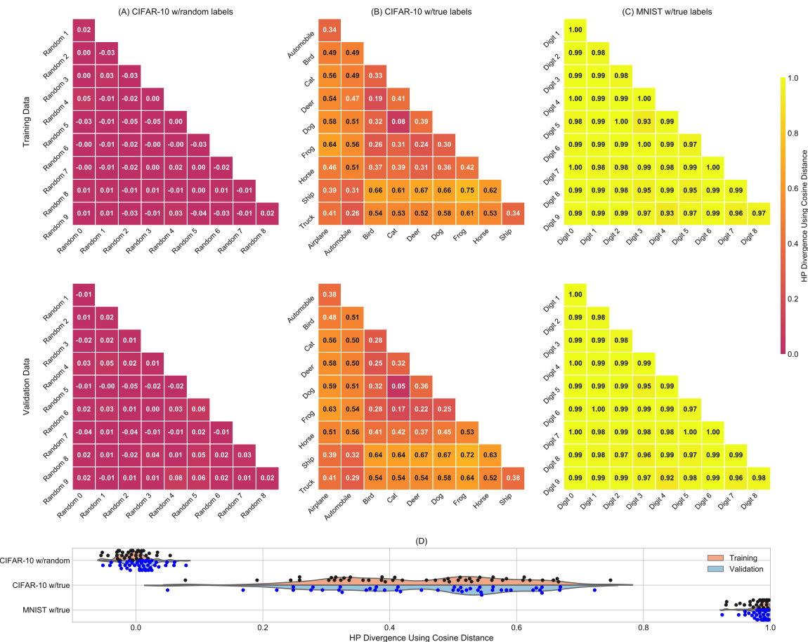
Figure S-17: Pairwise class HP statistics using cosine distance (training data above, validation data below) computed on (A) CIFAR10 with random labels, (B) CIFAR10 with true labels, and (C) MNIST with true labels. (D) The $\boldsymbol{\mathcal{H}}^{(t)}$ (black dots above) and $\boldsymbol{\mathcal{H}}^{(v)}$ (blue dots, below) values and respective kernel-based density functions (orange = training, blue = validation) for each task which illustrate that the estimated class separation for each task in their respective ambient representations are quite distinct.

Figures S-18 through S-22 present the class-wise HP statistics of the training and validation samples of the CIFAR10 data with random labels as they pass through an associated model. Each figure plots the results for one of the five training instances discussed in Section 3 of the paper. The (a) subfigures show the data passing through the untrained models and the (b) subfigures show the data passing through the trained version of the models. Similarly, Figures S-23 through S-27 present plots for the 5 model instances trained on the CIFAR10 data with true labels, and Figures S-28 through S-32 show the plots for the 5 MNIST-trained models. As mentioned above, the cosine distance is used for all of these cases.

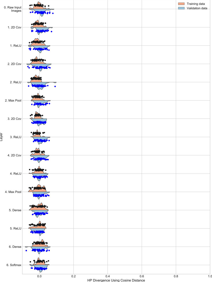
(a) Untrained model

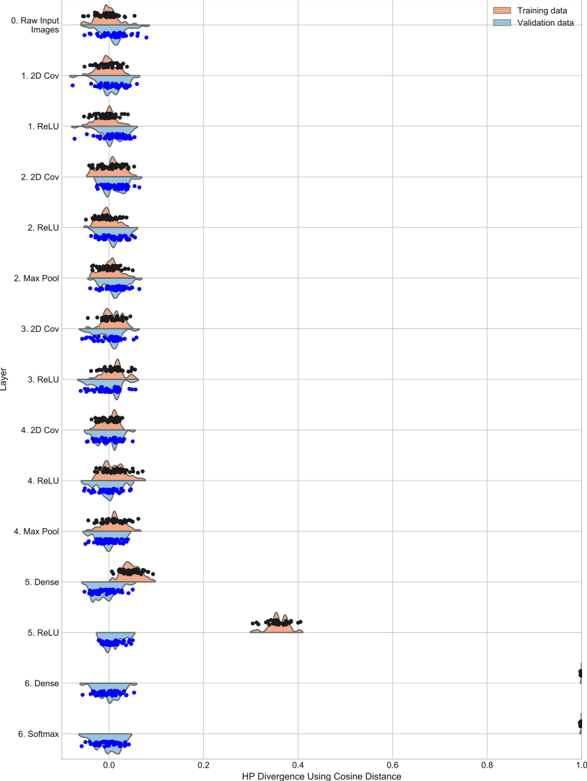
(b) Trained model

Figure S-18: $\mathcal{H}$ class-pair statistics at each layer for instance 1 of the model for CIFAR10 with random class labels. (a) shows results for the data for passing through the randomly initialized model (epoch 0 state). (b) shows the results for the data passing through the fully trained model (epoch 200 state). (Note: Cosine distance is used as the proximity measure.)

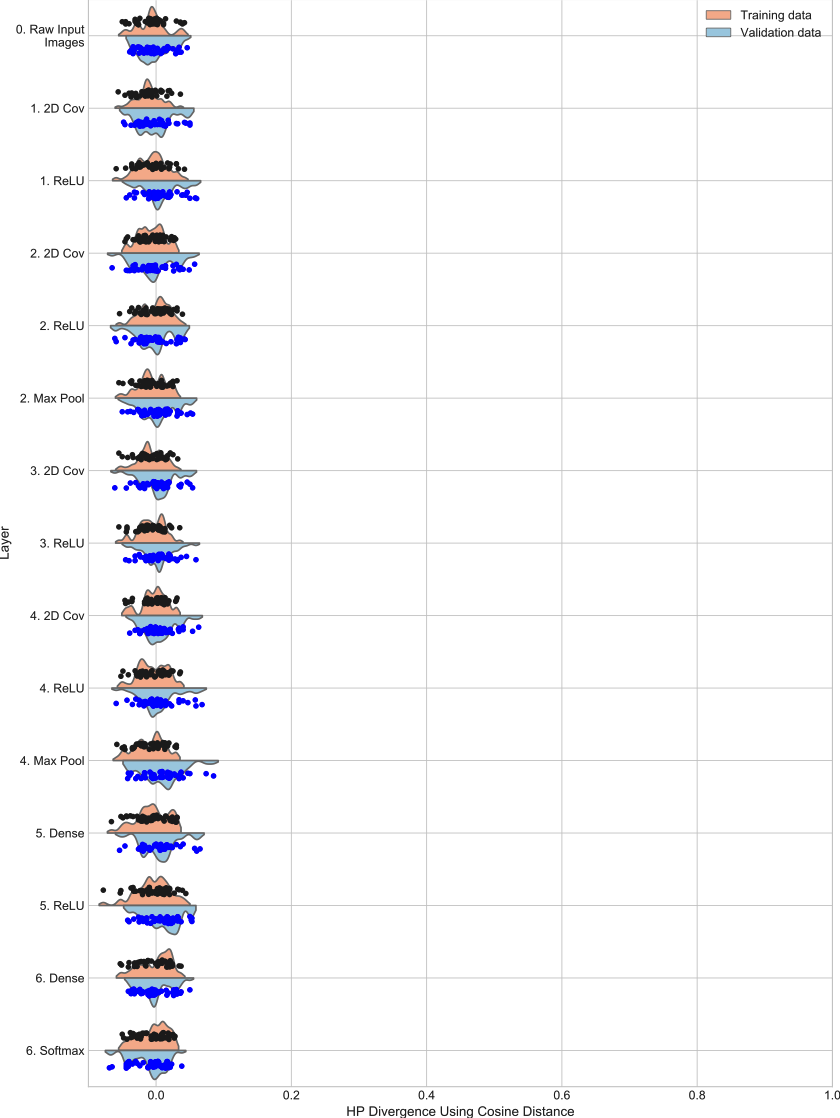
(a) Untrained model

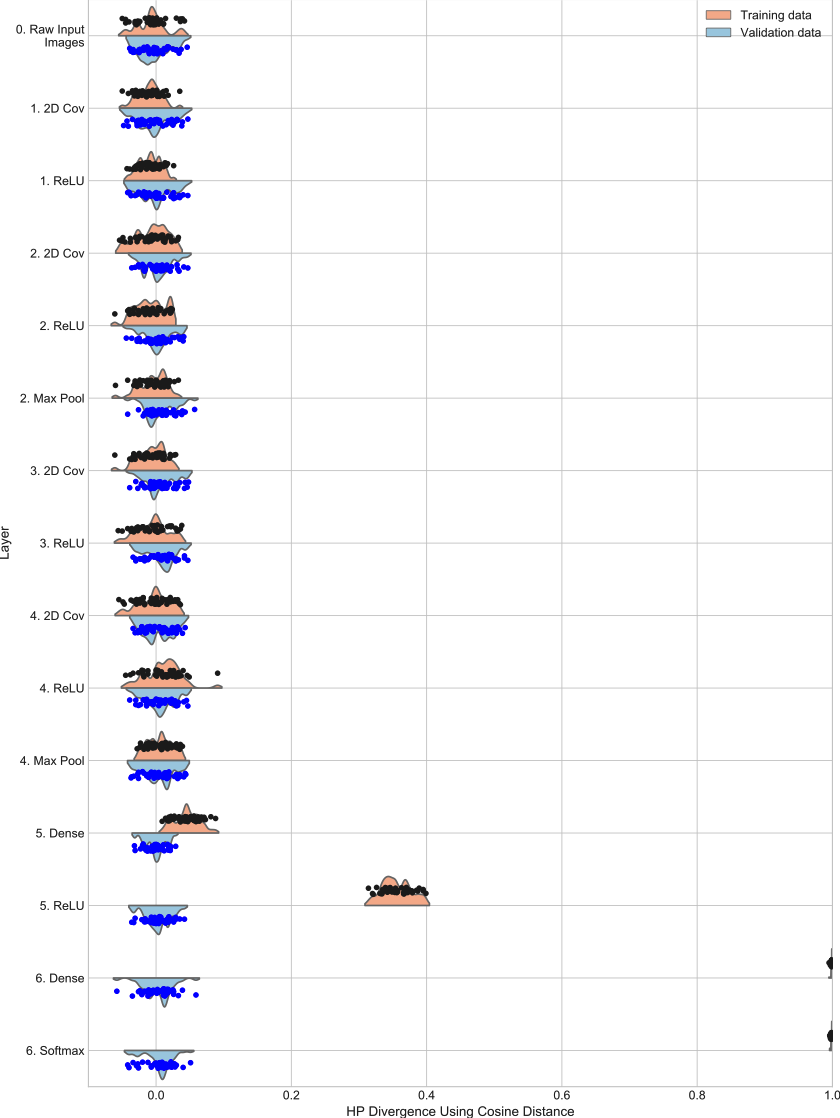
(b) Trained model

Figure S-19: $\mathcal{H}$ class-pair statistics at each layer for instance 2 of the model for CIFAR10 with random class labels. (a) shows results for the data for passing through the randomly initialized model (epoch 0 state). (b) shows the results for the data passing through the fully trained model (epoch 200 state). (Note: Cosine distance is used as the proximity measure.)

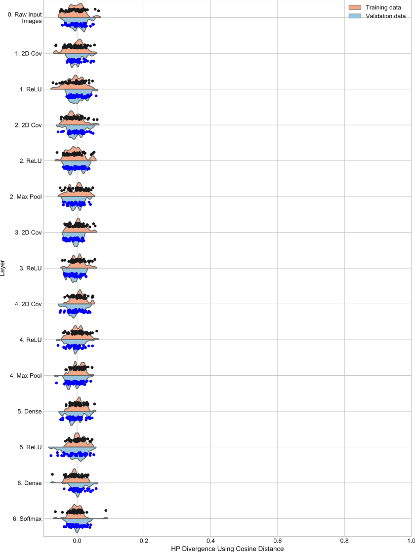
(a) Untrained model

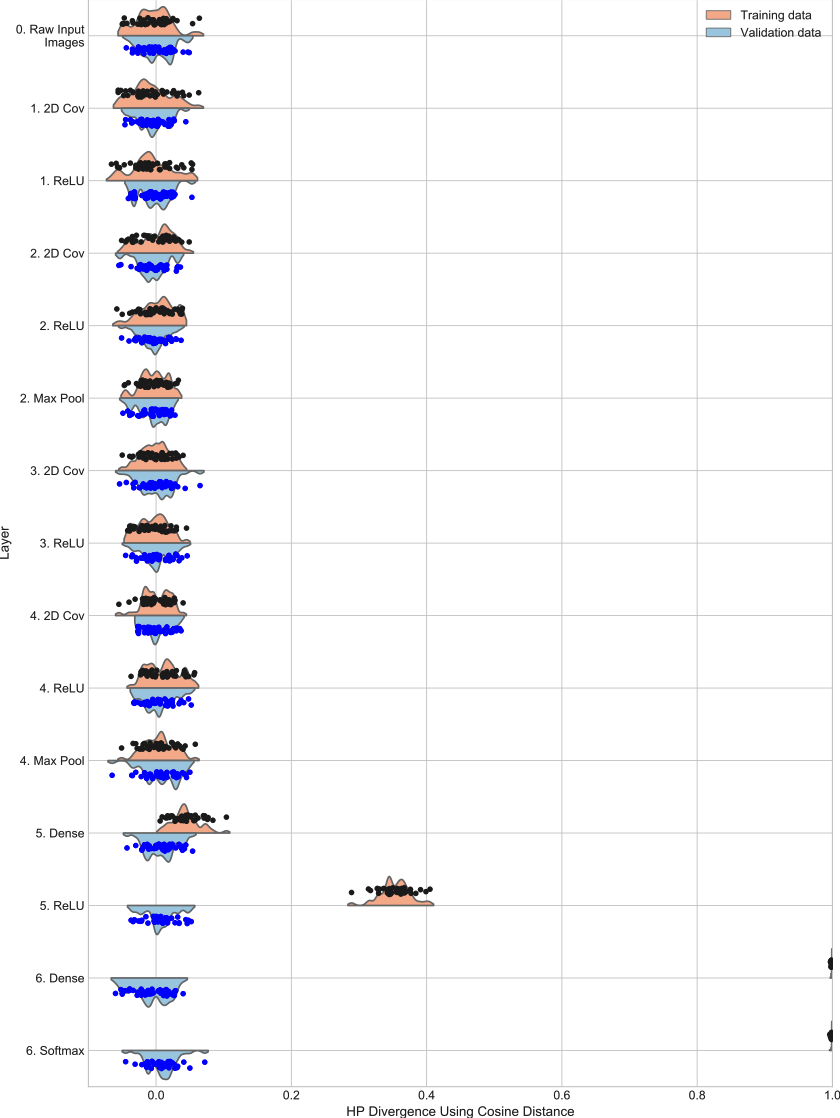
(b) Trained model

Figure S-20: $\mathcal{H}$ class-pair statistics at each layer for instance 3 of the model for CIFAR10 with random class labels. (a) shows results for the data for passing through the randomly initialized model (epoch 0 state). (b) shows the results for the data passing through the fully trained model (epoch 200 state). (Note: Cosine distance is used as the proximity measure.)

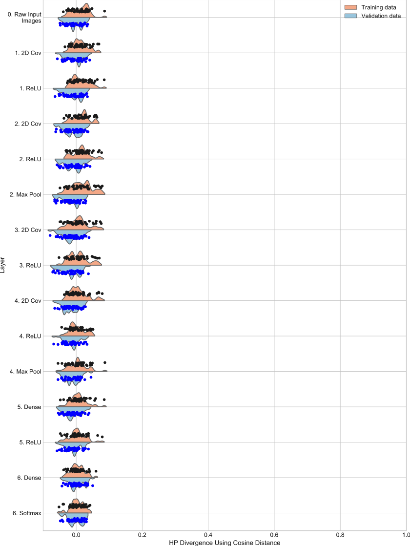
(a) Untrained model

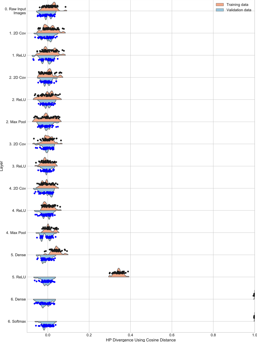
(b) Trained model

Figure S-21: $\mathcal{H}$ class-pair statistics at each layer for instance 4 of the model for CIFAR10 with random class labels. (a) shows results for the data for passing through the randomly initialized model (epoch 0 state). (b) shows the results for the data passing through the fully trained model (epoch 200 state). (Note: Cosine distance is used as the proximity measure.)

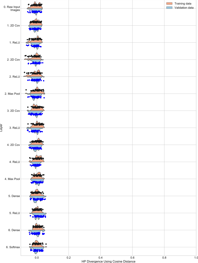
(a) Untrained model

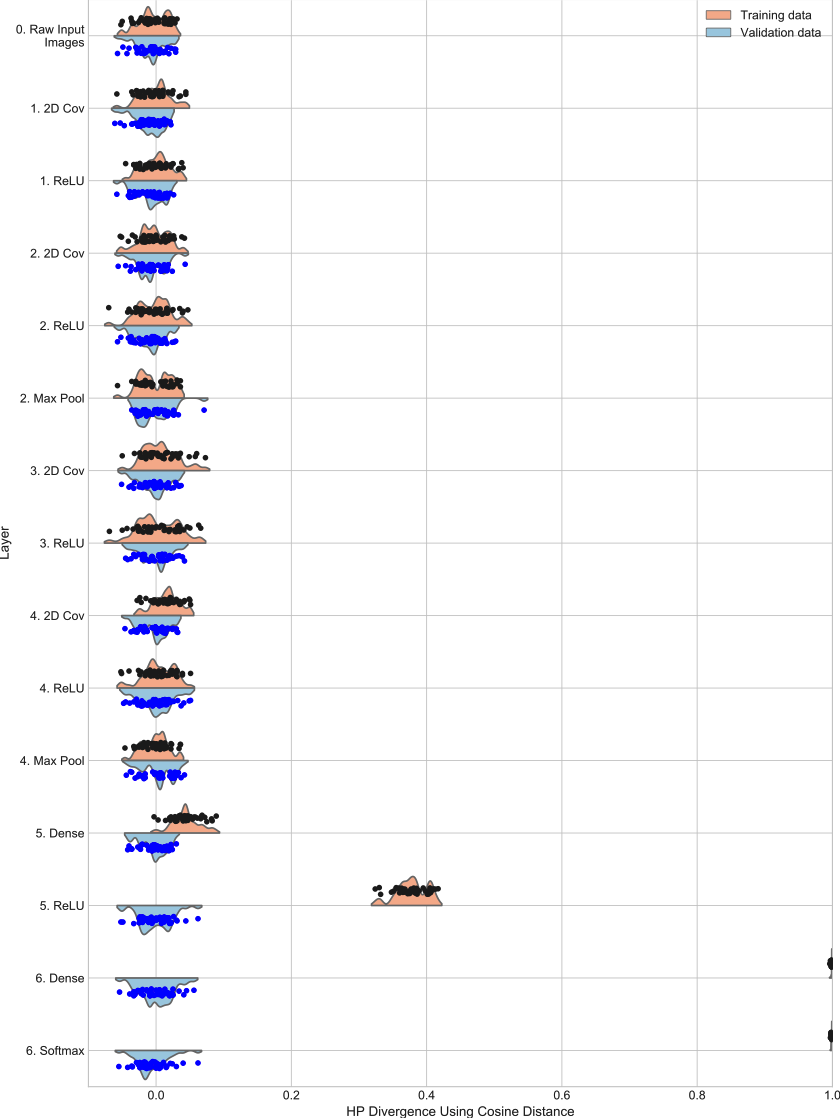
(b) Trained model

Figure S-22: $\mathcal{H}$ class-pair statistics at each layer for instance 5 of the model for CIFAR10 with random class labels. (a) shows results for the data for passing through the randomly initialized model (epoch 0 state). (b) shows the results for the data passing through the fully trained model (epoch 200 state). (Note: Cosine distance is used as the proximity measure.)

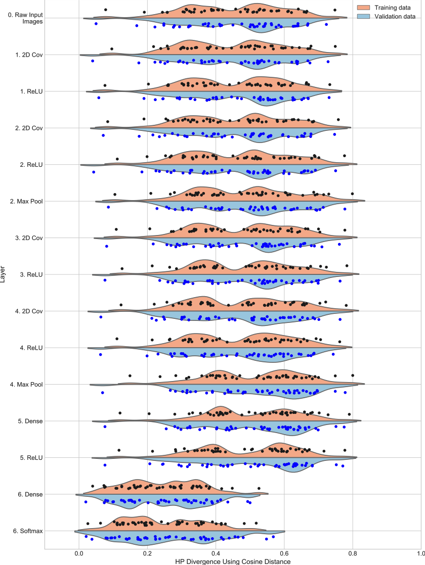
(a) Untrained model

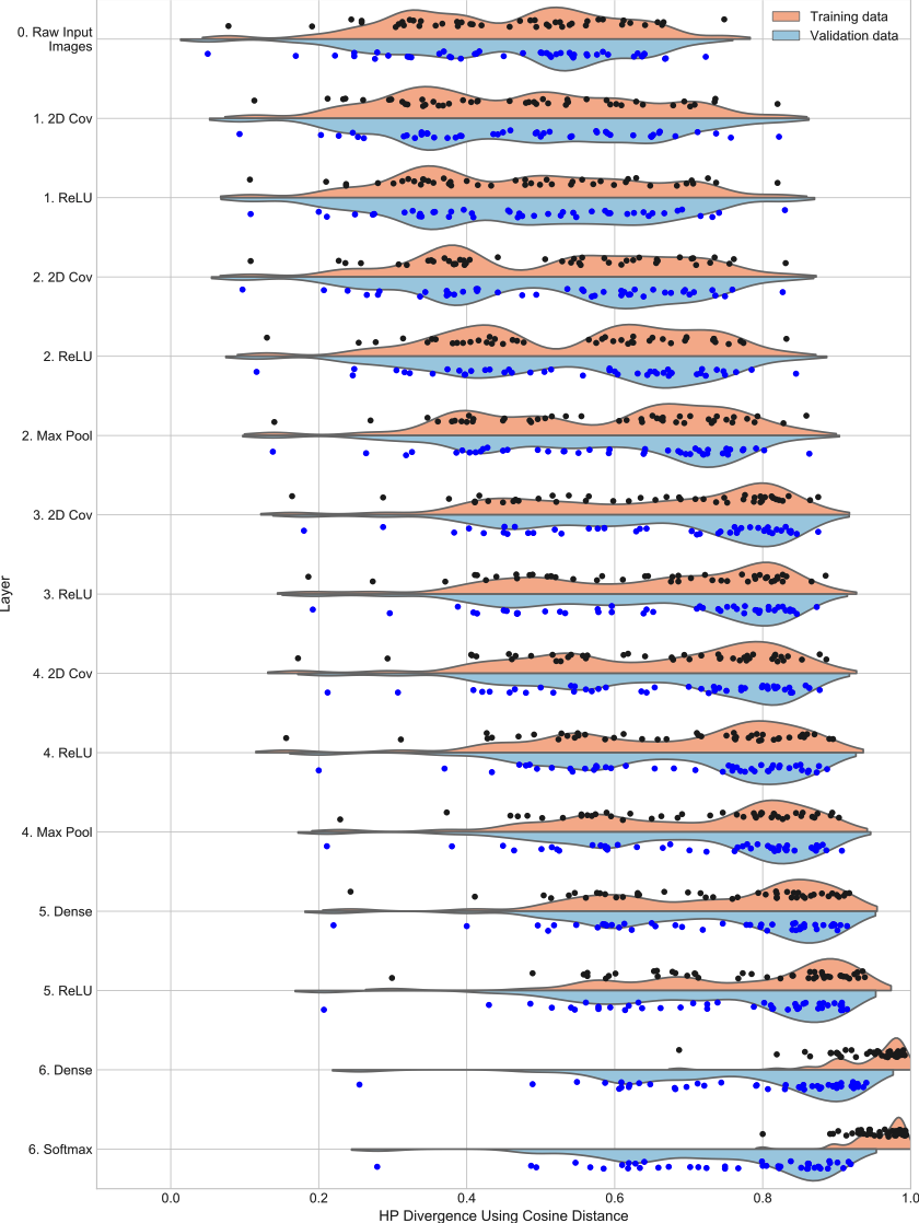
(b) Trained model

Figure S-23: $\mathcal{H}$ class-pair statistics at each layer for instance 1 of the model for CIFAR10 with true class labels. (a) shows results for the data for passing through the randomly initialized model (epoch 0 state). (b) shows the results for the data passing through the fully trained model (stopping at peak validation set accuracy). (Note: Cosine distance is used as the proximity measure.)

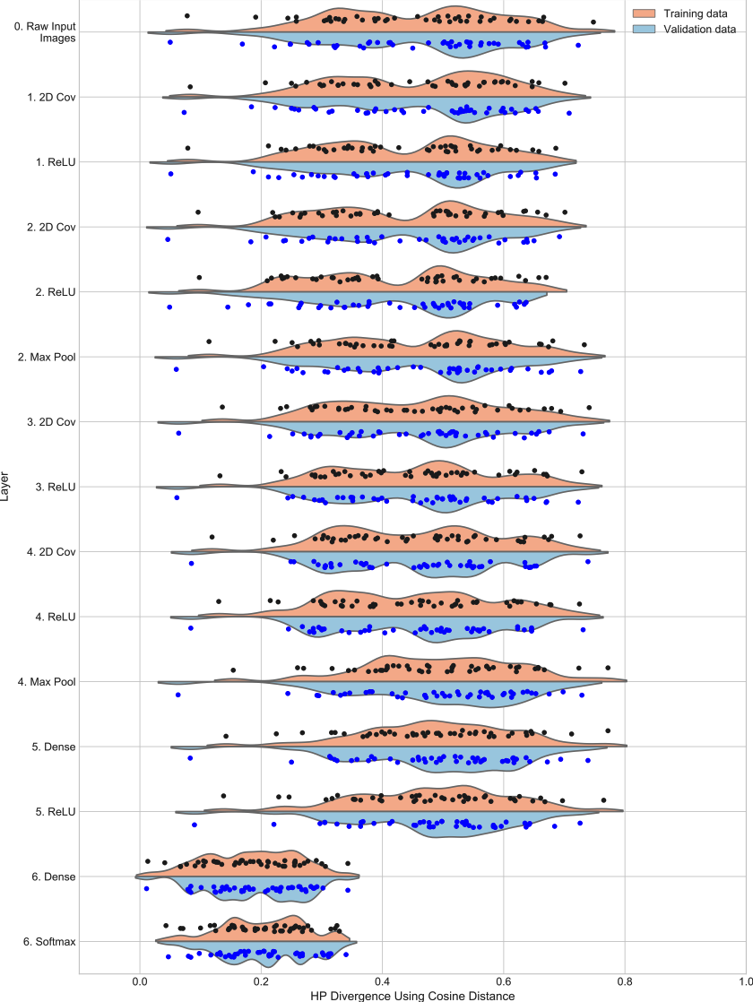
(a) Untrained model

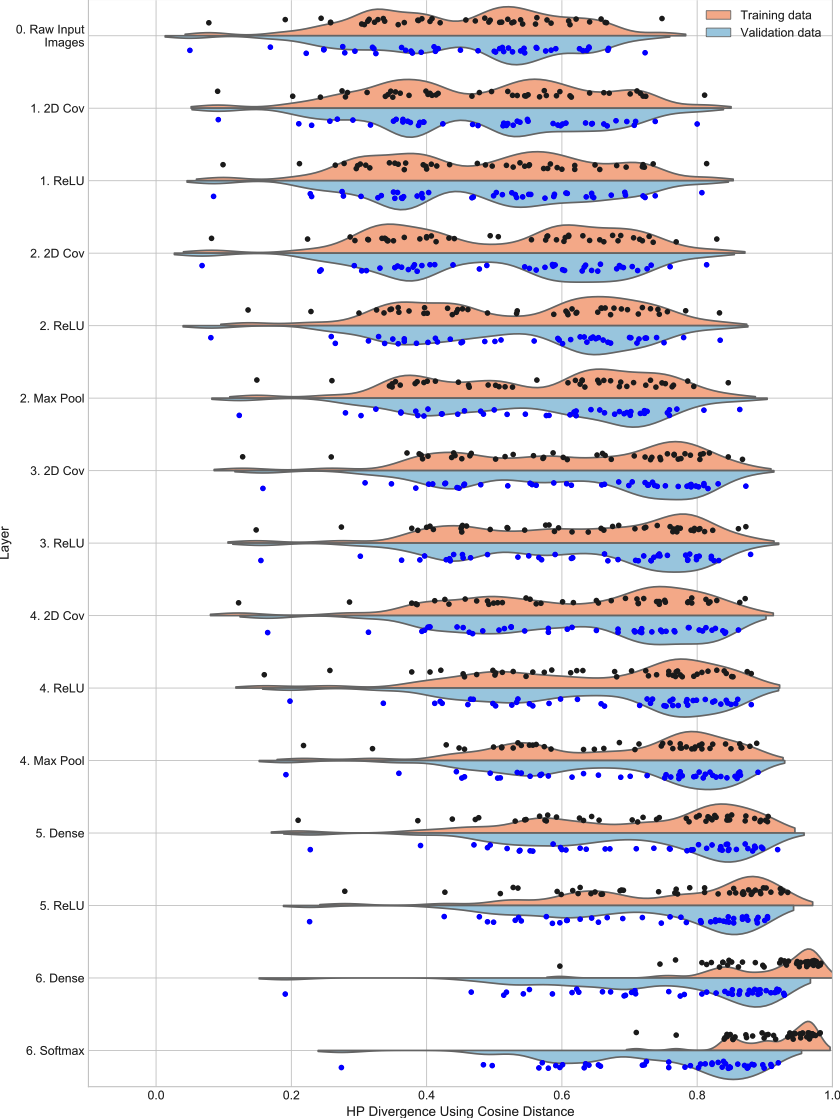
(b) Trained model

Figure S-24: $\mathcal{H}$ class-pair statistics at each layer for instance 2 of the model for CIFAR10 with true class labels. (a) shows results for the data for passing through the randomly initialized model (epoch 0 state). (b) shows the results for the data passing through the fully trained model (stopping at peak validation set accuracy). (Note: Cosine distance is used as the proximity measure.)

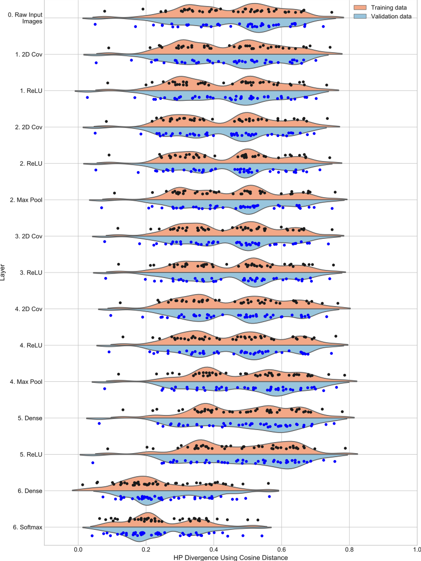
(a) Untrained model

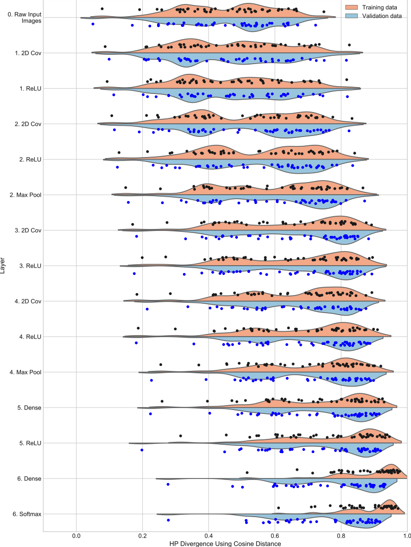
(b) Trained model

Figure S-25: $\mathcal{H}$ class-pair statistics at each layer for instance 3 of the model for CIFAR10 with true class labels. (a) shows results for the data for passing through the randomly initialized model (epoch 0 state). (b) shows the results for the data passing through the fully trained model (stopping at peak validation set accuracy). (Note: Cosine distance is used as the proximity measure.)

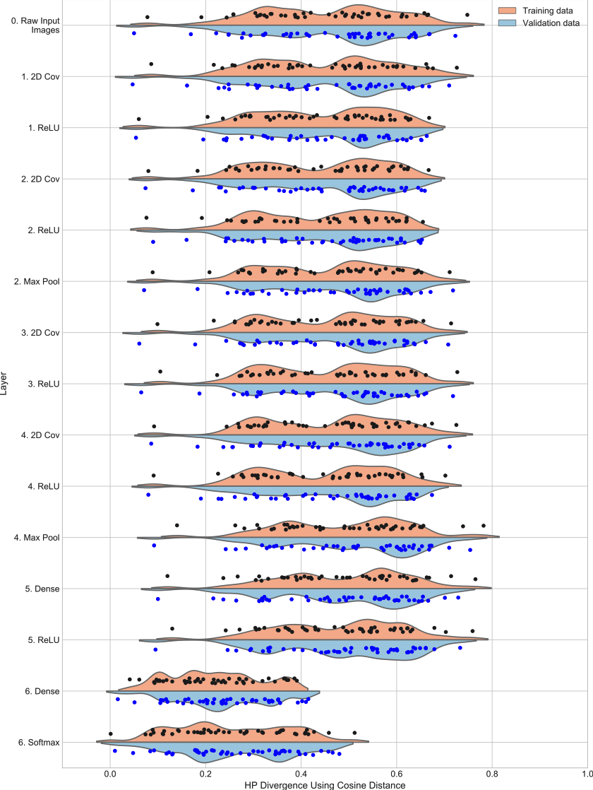
(a) Untrained model

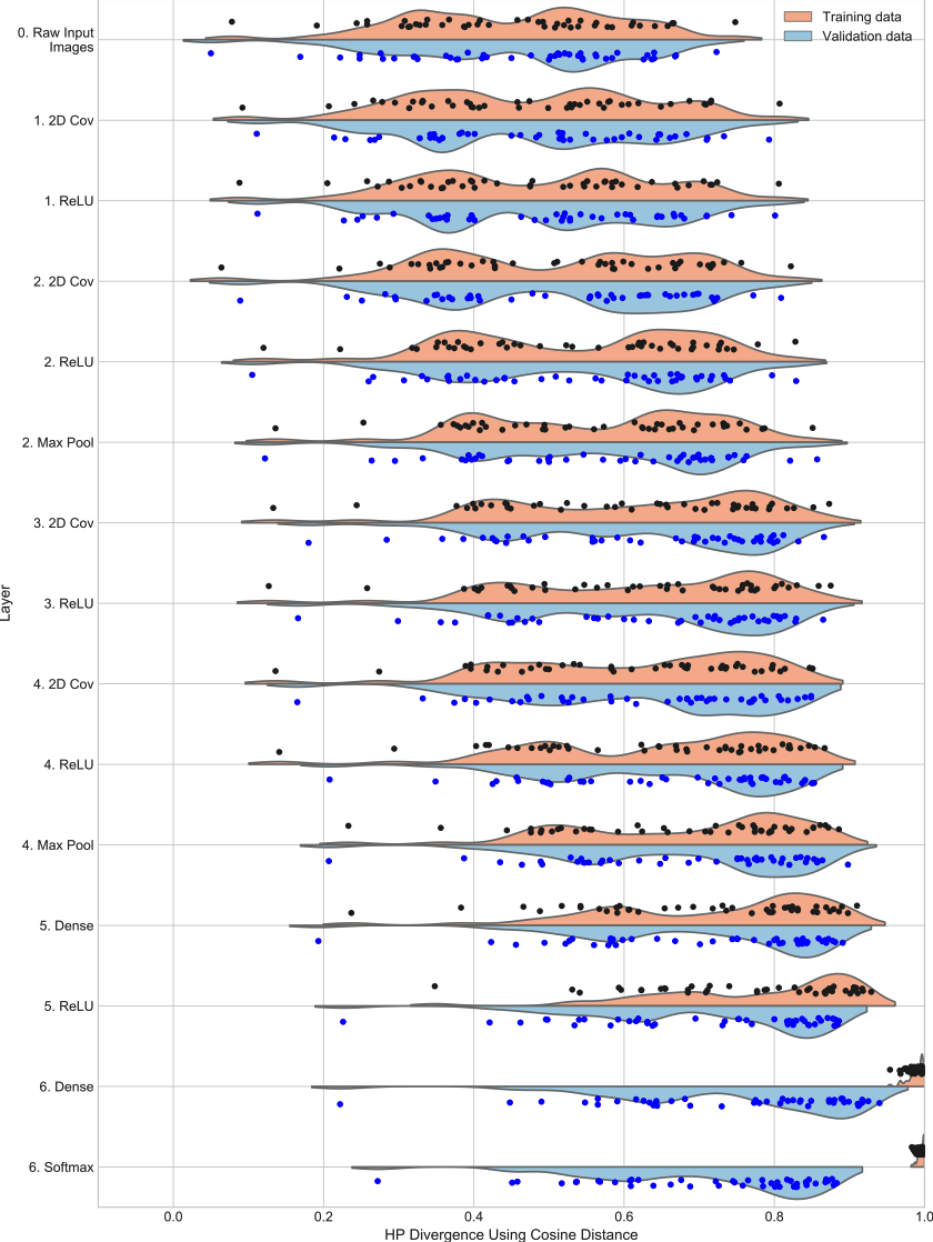
(b) Trained model

Figure S-26: $\mathcal{H}$ class-pair statistics at each layer for instance 4 of the model for CIFAR10 with true class labels. (a) shows results for the data for passing through the randomly initialized model (epoch 0 state). (b) shows the results for the data passing through the fully trained model (stopping at peak validation set accuracy). (Note: Cosine distance is used as the proximity measure.)

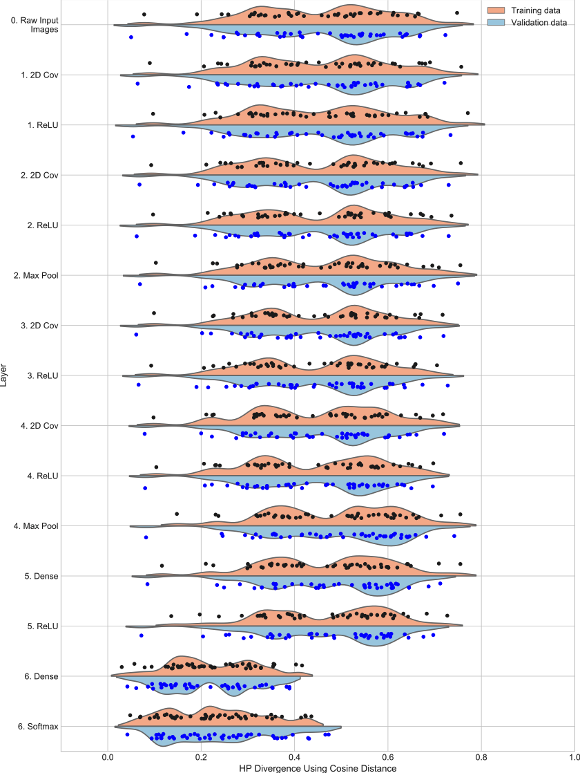
(a) Untrained model

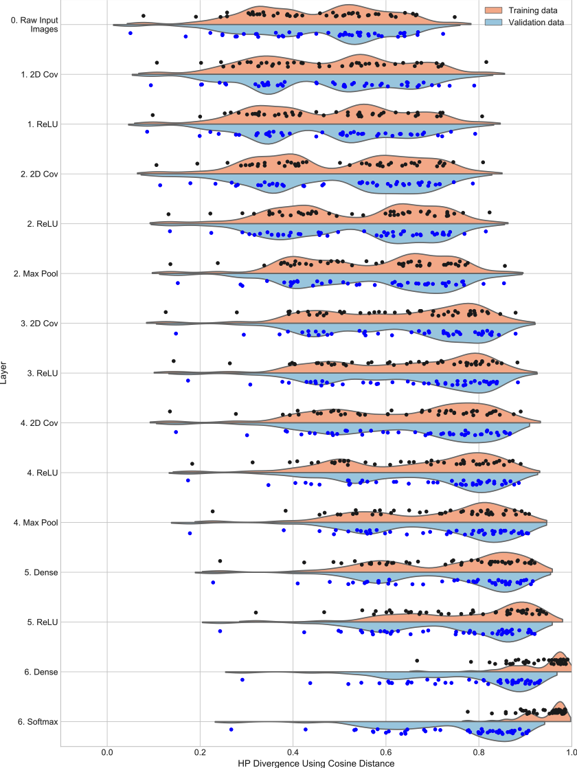
(b) Trained model

Figure S-27: $\mathcal{H}$ class-pair statistics at each layer for instance 5 of the model for CIFAR10 with true class labels. (a) shows results for the data for passing through the randomly initialized model (epoch 0 state). (b) shows the results for the data passing through the fully trained model (stopping at peak validation set accuracy). (Note: Cosine distance is used as the proximity measure.)

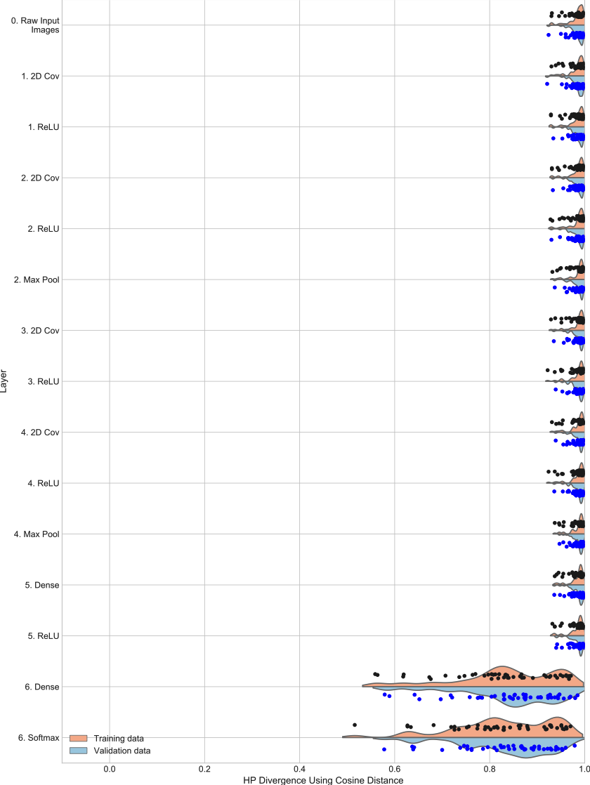
(a) Untrained model

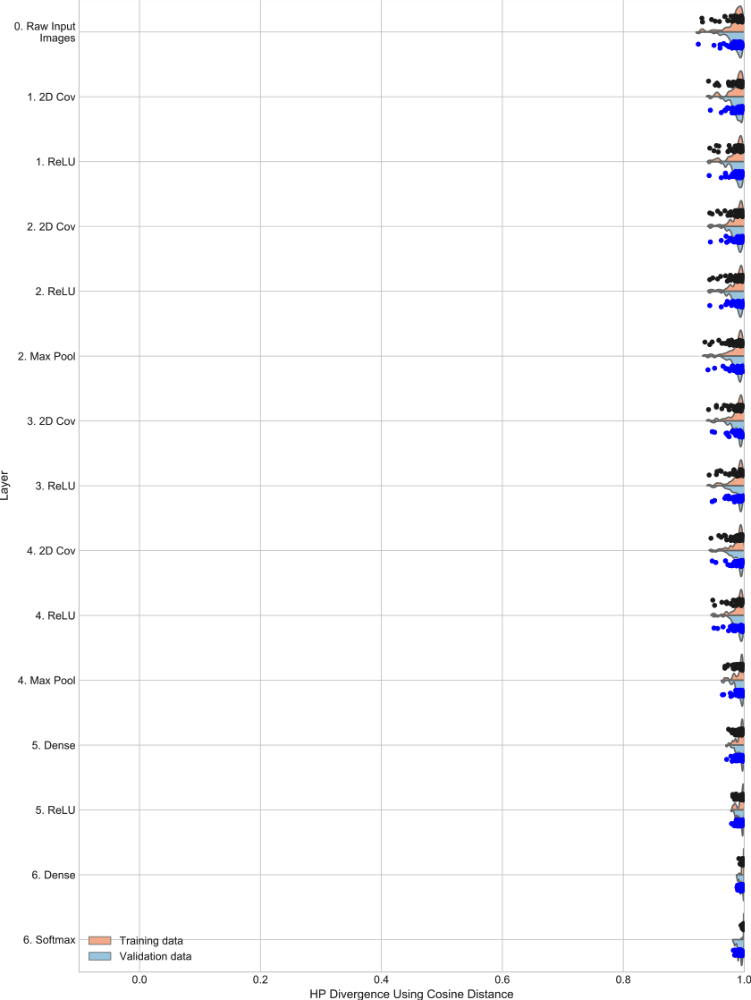
(b) Trained model

Figure S-28: $\mathcal{H}$ class-pair statistics at each layer for instance 1 of the model for MNIST with true class labels. (a) shows results for the data for passing through the randomly initialized model (epoch 0 state). (b) shows the results for the data passing through the fully trained model (stopping at peak validation set accuracy). (Note: Cosine distance is used as the proximity measure.)

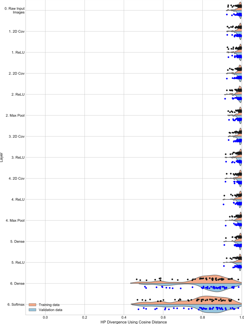
(a) Untrained model

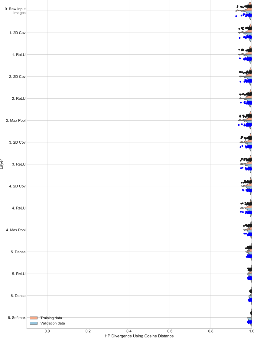
(b) Trained model

Figure S-29: $\mathcal{H}$ class-pair statistics at each layer for instance 2 of the model for MNIST with true class labels. (a) shows results for the data for passing through the randomly initialized model (epoch 0 state). (b) shows the results for the data passing through the fully trained model (stopping at peak validation set accuracy). (Note: Cosine distance is used as the proximity measure.)

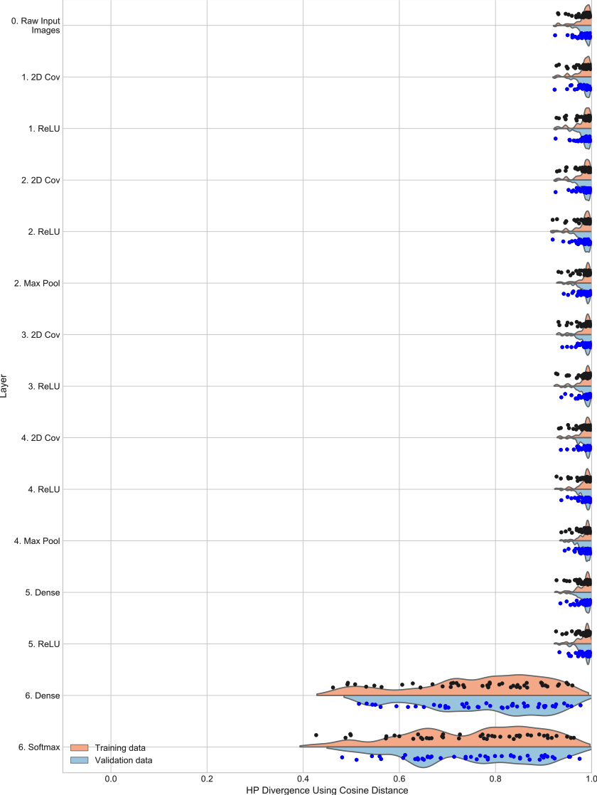
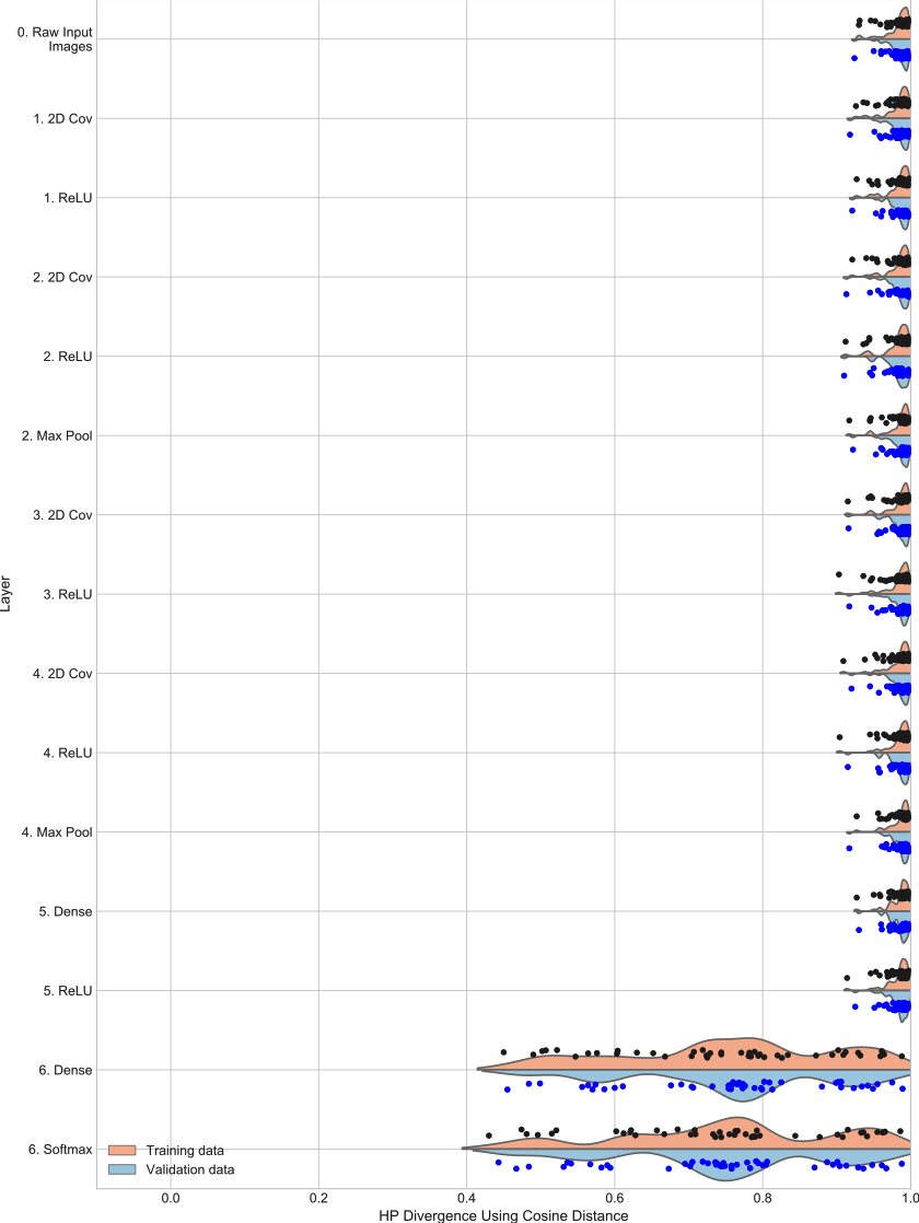
(a) Untrained model

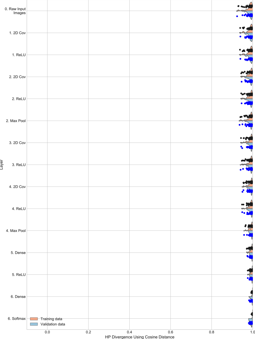
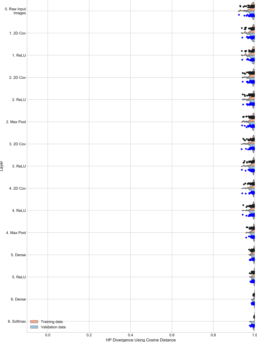
(b) Trained model

Figure S-30: $\mathcal{H}$ class-pair statistics at each layer for instance 3 of the model for MNIST with true class labels. (a) shows results for the data for passing through the randomly initialized model (epoch 0 state). (b) shows the results for the data passing through the fully trained model (stopping at peak validation set accuracy). (Note: Cosine distance is used as the proximity measure.)

(a) Untrained model

(b) Trained model

Figure S-31: $\mathcal{H}$ class-pair statistics at each layer for instance 4 of the model for MNIST with true class labels. (a) shows results for the data for passing through the randomly initialized model (epoch 0 state). (b) shows the results for the data passing through the fully trained model (stopping at peak validation set accuracy). (Note: Cosine distance is used as the proximity measure.)

(a) Untrained model

(b) Trained model

Figure S-32: $\mathcal{H}$ class-pair statistics at each layer for instance 5 of the model for MNIST with true class labels. (a) shows results for the data for passing through the randomly initialized model (epoch 0 state). (b) shows the results for the data passing through the fully trained model (stopping at peak validation set accuracy). (Note: Cosine distance is used as the proximity measure.)

Tables S-10 through S-18 present results of two-sample null hypothesis test of the difference of means, where cosine distance is used in the HP divergence calculations. The tables flag cases where the estimated $p$-values are $<0.025$.

Table S-10: Two-sided permutation test of training data to detect change in $\bar{\mathcal{H}}$ between layers (before training) with critical value $\alpha=0.025$. Red font denote layer instances for which we reject $\mathbf{H_{0}}$, black font denotes layers for which we fail to reject $\mathbf{H_{0}}$  (Eq. 14 in paper). (Note: Cosine distance is used as the proximity measure. 50,000 Monte Carlo trials were used to estimate the $p$-values. $\Delta{\bar{\mathcal{H}}}=\bar{\mathcal{H}}^{(t)}_{(k,0)}-\bar{\mathcal{H}}^{(t)}_{(k-1,0)}$))

Input Space	Output Space	CIFAR10 w Random		CIFAR10 w True		MNIST w True
		$\Delta{\bar{\mathcal{H}}}$	p-values	$\Delta{\bar{\mathcal{H}}}$	p-values	$\Delta{\bar{\mathcal{H}}}$	p-values
0.Input	1.Conv	-.001; -.004; -.001; -.002; -.001	.855; .302; .923; .736; .838	-.004; .002; -.011; -.002; .003	.901; .956; .725; .942; .932	.001; .000; -.001; -.000; -.000	.827; .978; .793; .991; .994
1.Conv	1.ReLU	-.006; .005; -.003; .002; -.002	.158; .211; .619; .675; .719	.007; -.017; -.006; -.007; -.001	.828; .567; .843; .806; .973	-.000; .001; .000; .001; .000	.958; .870; .901; .754; .936
1.ReLU	2.Conv	-.001; -.002; .001; .001; -.003	.745; .725; .830; .893; .536	.005; -.001; -.000; -.007; -.004	.871; .984; .991; .821; .893	.000; -.000; -.000; -.001; -.001	.962; .948; .977; .854; .870
2.Conv	2.ReLU	-.004; .006; .001; .001; .000	.298; .148; .866; .924; .995	.002; -.014; .006; .001; .002	.947; .642; .848; .973; .940	.000; -.000; -.001; -.002; .000	.940; .905; .816; .644; .942
2.ReLU	2.MaxPool	.005; -.004; .006; .000; .010	.129; .337; .283; .960; .071	.016; .036; .011; .018; .012	.623; .236; .721; .537; .698	.001; .002; .003; .002; .001	.775; .658; .366; .522; .703
2.MaxPool	3.Conv	-.001; -.002; .001; -.008; -.000	.833; .627; .895; .220; .922	-.002; -.001; -.004; -.002; -.012	.958; .981; .897; .951; .690	-.000; .001; -.001; -.000; -.001	.984; .865; .876; .959; .836
3.Conv	3.ReLU	.000; .000; .003; -.002; .004	.899; .913; .519; .788; .405	.005; -.006; .008; .005; -.006	.883; .846; .793; .876; .832	-.001; -.001; -.001; -.001; .001	.844; .843; .851; .768; .827
3.ReLU	4.Conv	.003; .004; .003; .002; -.001	.403; .363; .525; .730; .811	-.008; .005; .005; .001; .004	.799; .863; .885; .974; .888	.001; .001; .000; .001; .001	.884; .783; .889; .872; .846
4.Conv	4.ReLU	.004; -.002; -.003; -.004; .003	.252; .692; .449; .411; .481	-.001; -.005; -.005; -.009; -.003	.983; .852; .868; .771; .931	-.001; -.001; -.000; .000; -.001	.880; .778; .920; .972; .862
4.ReLU	4.MaxPool	.002; -.005; .001; .002; -.001	.728; .280; .733; .660; .779	.041; .044; .034; .043; .037	.187; .120; .281; .143; .218	.000; .001; .001; .002; .002	.894; .711; .800; .643; .595
4.MaxPool	5.Dense	-.001; .004; -.001; .001; -.007	.796; .431; .828; .860; .096	-.010; -.007; .000; -.004; -.016	.734; .794; .997; .900; .594	-.001; -.001; -.002; -.001; -.001	.736; .742; .597; .828; .743
5.Dense	5.ReLU	.003; .002; .001; -.001; .005	.583; .773; .811; .856; .153	-.013; -.007; -.011; -.009; -.000	.673; .805; .730; .764; .993	-.001; -.002; -.001; -.001; -.001	.735; .575; .672; .664; .721
5.ReLU	6.Dense	.006; .003; -.009; -.001; .001	.205; .571; .058; .846; .812	-.243; -.297; -.231; -.261; -.244	.000; .000; .000; .000; .000	-.152; -.188; -.221; -.232; -.193	.000; .000; .000; .000; .000
6.Dense	6.Softmax	.000; -.004; .001; -.001; -.002	.997; .401; .827; .745; .661	.002; .020; .004; .035; .007	.942; .205; .885; .132; .726	-.003; -.015; -.011; -.001; -.001	.884; .594; .711; .963; .966

Table S-11: Differences between the trained and initialized $\boldsymbol{\mathcal{H}}$ class-pair statistics of a layer, and respective $p$-values for the corresponding one-sided permutation test  (Eq. 15 in paper). Red font denotes layer instances for which we reject $\mathbf{H_{0}}$, and black font denotes layers for which we fail to reject $\mathbf{H_{0}}$. (Note:  Cosine distance is used as the proximity measure. 50,000 Monte Carlo trials to estimate the $p$-values. $\Delta{\bar{\mathcal{H}}}=\bar{\mathcal{H}}^{(t)}_{(k,T)}-\bar{\mathcal{H}}^{(t)}_{(k,0)}$)

Output Space	CIFAR10 w Random		CIFAR10 w True		MNIST w True
	$\Delta{\bar{\mathcal{H}}}$	p-values	$\Delta{\bar{\mathcal{H}}}$	p-values	$\Delta{\bar{\mathcal{H}}}$	p-values
1.Conv	.003; .001; -.002; -.003; .003	.220; .394; .631; .674; .220	.020; .031; .022; .026; .020	.269; .173; .254; .211; .277	.002; .002; .003; .002; .003	.288; .241; .160; .231; .222
1.ReLU	.007; -.004; .001; -.006; .006	.055; .807; .409; .853; .094	.018; .050; .035; .042; .025	.297; .061; .147; .096; .222	.002; .002; .003; .002; .002	.275; .282; .183; .310; .227
2.Conv	.017; .001; .006; -.013; .006	.000; .406; .115; .989; .098	.049; .075; .076; .075; .050	.076; .014; .016; .013; .071	.002; .002; .004; .003; .003	.246; .229; .135; .209; .166
2.ReLU	.012; -.007; .007; -.016; .006	.000; .945; .087; .997; .116	.081; .116; .106; .100; .082	.008; .000; .001; .001; .008	.002; .003; .005; .004; .003	.271; .199; .095; .099; .177
2.MaxPool	.014; .001; -.003; -.017; -.001	.000; .441; .726; .993; .607	.105; .108; .139; .111; .101	.001; .001; .000; .001; .001	-.000; .000; -.000; .001; .001	.550; .473; .505; .436; .393
3.Conv	.021; .001; -.001; -.005; .007	.000; .430; .585; .822; .080	.164; .154; .196; .158; .168	.000; .000; .000; .000; .000	.001; .001; .002; .003; .003	.327; .343; .270; .213; .203
3.ReLU	.023; .002; -.008; -.011; -.001	.000; .348; .966; .972; .552	.164; .169; .199; .162; .188	.000; .000; .000; .000; .000	.002; .002; .003; .004; .002	.293; .269; .212; .155; .249
4.Conv	.010; -.000; -.005; -.012; .012	.003; .506; .892; .984; .002	.178; .164; .193; .154; .186	.000; .000; .000; .000; .000	.002; .002; .004; .005; .003	.245; .219; .105; .066; .168
4.ReLU	.016; .015; .008; -.002; -.001	.000; .002; .051; .633; .597	.203; .200; .224; .194; .212	.000; .000; .000; .000; .000	.003; .004; .005; .005; .004	.149; .114; .061; .061; .074
4.MaxPool	.014; .016; .001; .003; -.006	.002; .000; .428; .255; .930	.188; .183; .214; .185; .214	.000; .000; .000; .000; .000	.006; .005; .006; .006; .005	.012; .020; .004; .007; .024
5.Dense	.052; .051; .041; .033; .046	.000; .000; .000; .000; .000	.231; .227; .244; .227; .264	.000; .000; .000; .000; .000	.008; .008; .009; .008; .007	.000; .001; .000; .000; .001
5.ReLU	.362; .360; .350; .337; .375	.000; .000; .000; .000; .000	.286; .277; .293; .297; .309	.000; .000; .000; .000; .000	.011; .011; .012; .010; .010	.000; .000; .000; .000; .000
6.Dense	.995; 1.000; 1.003; .994; .995	.000; .000; .000; .000; .000	.698; .725; .637; .770; .706	.000; .000; .000; .000; .000	.167; .203; .238; .247; .207	.000; .000; .000; .000; .000
6.Softmax	.995; 1.004; 1.002; .996; .997	.000; .000; .000; .000; .000	.709; .714; .638; .741; .709	.000; .000; .000; .000; .000	.171; .219; .250; .249; .209	.000; .000; .000; .000; .000

Table S-12: Training data difference between input and output of each layer’s $\boldsymbol{\mathcal{H}}$ class-pair statistics for the trained models, and respective $p$-values for the one sided permutation test (Eq. 17 in paper). Red font denotes layer instances for which we reject $\mathbf{H_{0}}$, and black font denotes layers for which we fail to reject $\mathbf{H_{0}}$. (Note:  Cosine distance is used as the proximity measure. 50,000 Monte Carlo trials used to estimate the $p$-values. $\Delta{\bar{\mathcal{H}}}=\bar{\mathcal{H}}^{(t)}_{(k,T)}-\bar{\mathcal{H}}^{(t)}_{(k-1,T)}$)

Input Space	Output Space	CIFAR10 w Random		CIFAR10 w True		MNIST w True
		$\Delta{\bar{\mathcal{H}}}$	p-values	$\Delta{\bar{\mathcal{H}}}$	p-values	$\Delta{\bar{\mathcal{H}}}$	p-values
0.Input	1.Conv	.002; -.003; -.002; -.004; .002	.296; .794; .667; .767; .292	.016; .032; .011; .024; .023	.312; .163; .366; .231; .247	.003; .002; .002; .002; .003	.214; .230; .237; .231; .220
1.Conv	1.ReLU	-.002; .001; .001; -.002; .001	.686; .408; .467; .603; .414	.004; .003; .007; .008; .004	.457; .468; .422; .398; .459	-.000; .000; .000; .000; .000	.511; .487; .465; .469; .477
1.ReLU	2.Conv	.009; .003; .006; -.006; -.003	.028; .236; .154; .825; .731	.037; .024; .040; .027; .021	.153; .249; .133; .221; .271	.000; .000; .000; .000; .000	.441; .467; .440; .450; .466
2.Conv	2.ReLU	-.008; -.002; .002; -.003; .000	.969; .685; .368; .667; .478	.034; .027; .036; .026; .034	.169; .221; .161; .235; .169	.000; .000; -.000; .000; .000	.494; .501; .499; .491; .480
2.ReLU	2.MaxPool	.007; .004; -.004; -.001; .002	.050; .193; .818; .544; .361	.040; .028; .043; .028; .031	.132; .216; .121; .205; .186	-.001; -.001; -.001; -.001; -.001	.669; .630; .669; .682; .617
2.MaxPool	3.Conv	.006; -.002; .002; .004; .008	.065; .683; .291; .257; .063	.057; .045; .053; .045; .054	.060; .108; .081; .103; .063	.002; .002; .001; .002; .001	.289; .302; .307; .268; .359
3.Conv	3.ReLU	.002; .002; -.004; -.007; -.004	.290; .368; .826; .919; .745	.005; .009; .012; .009; .014	.443; .399; .379; .404; .357	-.000; .000; -.000; -.000; .000	.548; .487; .498; .524; .463
3.ReLU	4.Conv	-.010; .002; .006; .001; .012	.994; .350; .103; .424; .016	.006; .000; -.001; -.007; .002	.437; .501; .509; .581; .475	.001; .001; .002; .002; .001	.375; .318; .279; .246; .315
4.Conv	4.ReLU	.010; .013; .010; .006; -.010	.011; .006; .017; .118; .987	.024; .031; .025; .031; .024	.250; .204; .240; .193; .263	.001; .000; .001; .000; .001	.398; .431; .405; .459; .373
4.ReLU	4.MaxPool	-.000; -.005; -.006; .007; -.006	.504; .832; .885; .051; .903	.026; .028; .024; .034; .039	.227; .217; .247; .162; .133	.003; .003; .003; .003; .002	.089; .116; .107; .095; .155
4.MaxPool	5.Dense	.037; .040; .039; .031; .046	.000; .000; .000; .000; .000	.032; .036; .030; .037; .034	.170; .150; .184; .128; .153	.002; .002; .001; .001; .002	.176; .169; .224; .258; .157
5.Dense	5.ReLU	.312; .310; .310; .303; .334	.000; .000; .000; .000; .000	.043; .043; .038; .062; .044	.091; .102; .124; .022; .085	.001; .002; .001; .001; .002	.161; .065; .127; .163; .091
5.ReLU	6.Dense	.640; .643; .645; .657; .620	.000; .000; .000; .000; .000	.169; .151; .113; .211; .153	.000; .000; .000; .000; .000	.004; .003; .004; .004; .004	.000; .000; .000; .000; .000
6.Dense	6.Softmax	-.000; -.000; -.000; .000; -.000	.945; .809; .515; .523; .652	.013; .009; .005; .007; .010	.102; .267; .398; .000; .206	.001; .001; .001; .001; .001	.000; .000; .000; .016; .000

Table S-13: Training data difference between between multi-layer component input and output $\boldsymbol{\mathcal{H}}$ class-pair statistics for the trained models, and respective $p$-values for the one sided permutation test (Eq. 17 in paper). Red font denotes layer instances for which we reject $\mathbf{H_{0}}$, and black font denotes layers for which we fail to reject $\mathbf{H_{0}}$. (Note:  Cosine distance is used as the proximity measure. 50,000 Monte Carlo trials used to estimate the $p$-values. $\Delta{\bar{\mathcal{H}}}=\bar{\mathcal{H}}^{(t)}_{(k_{2},T)}-\bar{\mathcal{H}}^{(t)}_{(k_{1},T)}$)

Input Space	Output Space	CIFAR10 w Random		CIFAR10 w True		MNIST w True
		$\Delta{\bar{\mathcal{H}}}$	p-values	$\Delta{\bar{\mathcal{H}}}$	p-values	$\Delta{\bar{\mathcal{H}}}$	p-values
0.Input	1.ReLU	.000; -.003; -.002; -.006; .004	.472; .739; .629; .838; .214	.020; .035; .018; .032; .026	.267; .145; .289; .165; .209	.003; .003; .003; .003; .003	.224; .214; .209; .210; .199
1.ReLU	2.ReLU	.000; .001; .008; -.009; -.003	.457; .426; .091; .910; .702	.071; .052; .077; .053; .056	.024; .071; .017; .066; .055	.000; .000; .000; .000; .000	.438; .466; .447; .438; .450
2.ReLU	2.MaxPool	.007; .004; -.004; -.001; .002	.049; .192; .819; .548; .353	.040; .028; .043; .028; .031	.135; .217; .118; .208; .184	-.001; -.001; -.001; -.001; -.001	.672; .628; .666; .684; .617
2.MaxPool	3.ReLU	.009; -.000; -.002; -.003; .004	.023; .545; .669; .695; .238	.062; .054; .064; .054; .068	.043; .068; .043; .064; .029	.001; .002; .001; .002; .001	.322; .292; .313; .293; .329
3.ReLU	4.ReLU	.000; .015; .016; .007; .001	.491; .002; .001; .078; .405	.030; .031; .024; .024; .026	.210; .202; .252; .252; .241	.002; .002; .002; .002; .002	.284; .256; .210; .217; .218
4.ReLU	4.MaxPool	-.000; -.005; -.006; .007; -.006	.507; .830; .882; .054; .902	.026; .028; .024; .034; .039	.224; .218; .248; .159; .133	.003; .003; .003; .003; .002	.087; .117; .106; .096; .154
4.MaxPool	5.ReLU	.349; .350; .349; .334; .380	.000; .000; .000; .000; .000	.075; .079; .068; .100; .079	.011; .010; .019; .001; .008	.003; .003; .003; .002; .003	.034; .011; .037; .059; .015
5.ReLU	6.Softmax	.639; .643; .645; .657; .620	.000; .000; .000; .000; .000	.182; .160; .118; .218; .163	.000; .000; .000; .000; .000	.005; .004; .005; .005; .004	.000; .000; .000; .000; .000

Table S-14: Training data difference between between multi-layer component input and output $\boldsymbol{\mathcal{H}}$ class-pair statistics for the trained models, and respective $p$-values for the one sided permutation test (Eq. 17 in paper). Red font denotes layer instances for which we reject $\mathbf{H_{0}}$, and black font denotes layers for which we fail to reject $\mathbf{H_{0}}$. (Note:  Cosine distance is used as the proximity measure. 50,000 Monte Carlo trials used to estimate the $p$-values. $\Delta{\bar{\mathcal{H}}}=\bar{\mathcal{H}}^{(t)}_{(k_{2},T)}-\bar{\mathcal{H}}^{(t)}_{(k_{1},T)}$)

Input Space	Output Space	CIFAR10 w Random		CIFAR10 w True		MNIST w True
		$\Delta{\bar{\mathcal{H}}}$	p-values	$\Delta{\bar{\mathcal{H}}}$	p-values	$\Delta{\bar{\mathcal{H}}}$	p-values
0.Input	2.MaxPool	.008; .002; .002; -.015; .003	.047; .328; .371; .992; .271	.131; .114; .139; .114; .113	.000; .000; .000; .000; .001	.002; .002; .002; .002; .002	.316; .295; .298; .314; .251
2.MaxPool	4.MaxPool	.009; .010; .008; .011; -.000	.031; .006; .046; .033; .537	.119; .112; .113; .113; .133	.000; .001; .001; .001; .000	.006; .006; .006; .006; .006	.012; .013; .007; .006; .013
4.MaxPool	5.ReLU	.349; .350; .349; .334; .380	.000; .000; .000; .000; .000	.075; .079; .068; .100; .079	.012; .010; .019; .001; .009	.003; .003; .003; .002; .003	.033; .011; .037; .059; .014
5.ReLU	6.Softmax	.639; .643; .645; .657; .620	.000; .000; .000; .000; .000	.182; .160; .118; .218; .163	.000; .000; .000; .000; .000	.005; .004; .005; .005; .004	.000; .000; .000; .000; .000

Table S-15: Validation data differences in mean of $\boldsymbol{\mathcal{H}}$ class-pair statistics between the input and output representations of a layer, and respective one-sided permutation test $p$-values. Red font denotes layer instances for which we reject $\mathbf{H_{0}}$, and black font denotes layers for which we fail to reject $\mathbf{H_{0}}$ (Eq. 18 in paper). (Note: Note:  Cosine distance is used as the proximity measure. 50,000 Monte Carlo trials used to estimate the $p$-values. $\Delta{\bar{\mathcal{H}}}=\bar{\mathcal{H}}^{(v)}_{(k,T)}-\bar{\mathcal{H}}^{(v)}_{(k-1,T)}$)

Input Space	Output Space	CIFAR10 w Random		CIFAR10 w True		MNIST w True
		$\Delta{\bar{\mathcal{H}}}$	p-values	$\Delta{\bar{\mathcal{H}}}$	p-values	$\Delta{\bar{\mathcal{H}}}$	p-values
0.Input	1.Conv	-.002; .001; -.005; -.001; -.000	.669; .395; .886; .577; .524	.017; .032; .008; .022; .017	.309; .168; .410; .245; .307	.003; .002; .002; .002; .002	.161; .206; .193; .194; .205
1.Conv	1.ReLU	.002; .000; .001; -.000; .001	.381; .490; .417; .517; .447	.006; -.001; .012; .009; .004	.423; .512; .371; .396; .455	.000; .000; .000; .000; .000	.483; .477; .470; .475; .497
1.ReLU	2.Conv	.003; .003; -.002; .002; -.000	.287; .249; .640; .346; .501	.035; .026; .042; .025; .023	.164; .227; .124; .238; .264	.000; .000; .000; .000; .000	.432; .435; .453; .478; .461
2.Conv	2.ReLU	-.003; .001; .001; -.000; -.002	.754; .432; .399; .503; .717	.030; .024; .029; .028; .032	.200; .259; .229; .219; .188	-.000; .000; -.000; -.000; .000	.517; .499; .512; .505; .496
2.ReLU	2.MaxPool	.004; .003; -.001; -.006; .007	.219; .267; .578; .895; .050	.044; .030; .048; .030; .038	.112; .201; .099; .196; .136	-.001; -.001; -.001; -.001; -.001	.635; .692; .667; .670; .665
2.MaxPool	3.Conv	-.012; .000; .005; .006; .001	.989; .462; .127; .090; .396	.064; .054; .060; .053; .061	.040; .068; .057; .069; .045	.001; .002; .002; .002; .002	.302; .237; .275; .234; .266
3.Conv	3.ReLU	-.003; .002; .001; -.002; .001	.721; .311; .427; .650; .437	.003; .005; .009; .004; .012	.466; .443; .405; .448; .370	-.000; -.000; -.000; -.000; .000	.513; .520; .529; .531; .479
3.ReLU	4.Conv	-.001; -.004; .000; -.002; -.001	.556; .826; .498; .706; .593	.006; .004; .004; -.002; .003	.436; .452; .458; .523; .474	.000; .001; .001; .001; .001	.448; .337; .340; .344; .410
4.Conv	4.ReLU	.002; .002; .003; -.000; .003	.313; .308; .273; .525; .267	.024; .030; .023; .032; .030	.245; .203; .252; .176; .211	.001; -.000; .000; .000; .001	.383; .509; .472; .427; .408
4.ReLU	4.MaxPool	-.001; -.001; .005; .002; .004	.598; .605; .180; .355; .204	.018; .024; .017; .028; .031	.295; .253; .309; .204; .192	.002; .003; .003; .002; .002	.143; .104; .084; .132; .118
4.MaxPool	5.Dense	-.007; -.005; -.002; -.003; -.006	.931; .881; .624; .719; .932	.025; .029; .023; .025; .020	.233; .204; .246; .231; .283	.001; .001; .001; .001; .002	.203; .156; .298; .178; .160
5.Dense	5.ReLU	.017; .003; -.000; .001; .001	.000; .166; .543; .450; .417	.009; .009; .012; .003; .009	.398; .400; .357; .461; .390	.001; .001; .001; .001; .001	.239; .201; .167; .271; .283
5.ReLU	6.Dense	-.007; -.001; -.013; -.007; .002	.938; .552; .996; .932; .371	.040; .039; .035; .041; .035	.112; .125; .145; .106; .143	.002; .001; .002; .001; .002	.009; .144; .046; .112; .057
6.Dense	6.Softmax	-.002; .003; .015; .010; -.008	.658; .274; .002; .020; .946	-.026; -.012; -.019; -.038; -.025	.793; .644; .727; .883; .787	-.003; -.002; -.003; -.004; -.003	.999; .990; .999; 1.000; 1.000

Table S-16: Validation data differences in mean of $\boldsymbol{\mathcal{H}}$ class-pair statistics between the input and output representations of multilayer layer compnents, and respective one-sided permutation test $p$-values. Red font denotes layer instances for which we reject $\mathbf{H_{0}}$, and black font denotes layers for which we fail to reject $\mathbf{H_{0}}$ (Eq. 18 in paper). (Note: Note:  Cosine distance is used as the proximity measure. 50,000 Monte Carlo trials used to estimate the $p$-values. $\Delta{\bar{\mathcal{H}}}=\bar{\mathcal{H}}^{(v)}_{(k_{2},T)}-\bar{\mathcal{H}}^{(v)}_{(k_{1},T)}$)

Input Space	Output Space	CIFAR10 w Random		CIFAR10 w True		MNIST w True
		$\Delta{\bar{\mathcal{H}}}$	p-values	$\Delta{\bar{\mathcal{H}}}$	p-values	$\Delta{\bar{\mathcal{H}}}$	p-values
0.Input	1.ReLU	-.001; .001; -.005; -.001; .000	.555; .381; .838; .593; .472	.023; .031; .020; .031; .021	.249; .176; .283; .174; .271	.003; .002; .003; .003; .002	.156; .188; .174; .183; .203
1.ReLU	2.ReLU	-.000; .004; -.001; .002; -.002	.527; .203; .549; .344; .715	.065; .050; .071; .053; .055	.036; .082; .025; .064; .063	.000; .000; .000; .000; .000	.451; .435; .467; .481; .460
2.ReLU	2.MaxPool	.004; .003; -.001; -.006; .007	.225; .272; .582; .892; .051	.044; .030; .048; .030; .038	.111; .199; .100; .198; .136	-.001; -.001; -.001; -.001; -.001	.638; .689; .670; .670; .658
2.MaxPool	3.ReLU	-.015; .003; .006; .005; .002	.997; .267; .079; .137; .341	.067; .059; .069; .057; .074	.034; .053; .034; .053; .021	.001; .002; .001; .002; .002	.318; .248; .300; .264; .251
3.ReLU	4.ReLU	.002; -.002; .003; -.003; .002	.380; .668; .275; .749; .354	.030; .034; .028; .030; .032	.198; .174; .223; .195; .186	.001; .001; .001; .001; .001	.331; .354; .319; .289; .323
4.ReLU	4.MaxPool	-.001; -.001; .005; .002; .004	.598; .603; .180; .349; .201	.018; .024; .017; .028; .031	.296; .248; .315; .205; .192	.002; .003; .003; .002; .002	.146; .105; .084; .131; .118
4.MaxPool	5.ReLU	.009; -.001; -.002; -.002; -.005	.016; .627; .655; .667; .877	.034; .038; .035; .028; .029	.166; .136; .149; .203; .200	.002; .002; .002; .002; .002	.070; .035; .068; .069; .069
5.ReLU	6.Softmax	-.009; .002; .001; .003; -.006	.973; .297; .380; .258; .896	.014; .027; .016; .004; .010	.329; .203; .306; .453; .377	-.000; -.001; -.001; -.002; -.002	.635; .894; .909; .990; .941

Table S-17: Validation data differences in mean of $\boldsymbol{\mathcal{H}}$ class-pair statistics between the input and output representations of multilayer layer compnents, and respective one-sided permutation test $p$-values. Red font denotes layer instances for which we reject $\mathbf{H_{0}}$, and black font denotes layers for which we fail to reject $\mathbf{H_{0}}$ (Eq. 18 in paper). (Note:  Cosine distance is used as the proximity measure. 50,000 Monte Carlo trials used to estimate the $p$-values. $\Delta{\bar{\mathcal{H}}}=\bar{\mathcal{H}}^{(v)}_{(k_{2},T)}-\bar{\mathcal{H}}^{(v)}_{(k_{1},T)}$)

Input Space	Output Space	CIFAR10 w Random		CIFAR10 w True		MNIST w True
		$\Delta{\bar{\mathcal{H}}}$	p-values	$\Delta{\bar{\mathcal{H}}}$	p-values	$\Delta{\bar{\mathcal{H}}}$	p-values
0.Input	2.MaxPool	.003; .008; -.006; -.005; .005	.309; .039; .907; .843; .119	.132; .111; .138; .115; .114	.000; .001; .000; .000; .001	.002; .002; .002; .002; .002	.215; .287; .279; .294; .298
2.MaxPool	4.MaxPool	-.014; -.000; .013; .004; .008	.999; .538; .003; .213; .049	.115; .117; .113; .115; .137	.000; .001; .001; .001; .000	.004; .005; .005; .005; .005	.022; .010; .009; .009; .008
4.MaxPool	5.ReLU	.009; -.001; -.002; -.002; -.005	.016; .624; .657; .670; .874	.034; .038; .035; .028; .029	.162; .139; .149; .200; .201	.002; .002; .002; .002; .002	.069; .036; .066; .069; .069
5.ReLU	6.Softmax	-.009; .002; .001; .003; -.006	.973; .300; .380; .264; .898	.014; .027; .016; .004; .010	.333; .202; .307; .451; .381	-.000; -.001; -.001; -.002; -.002	.634; .891; .909; .989; .942

Table S-18: Two-sided permutation test (Eq. 20 in paper) comparing the differences in the mean change induced on the training and validation statistics ( $\boldsymbol{\Delta{\mathcal{H}}}^{(t)}_{(k,k-1)}$ and $\boldsymbol{\Delta{\mathcal{H}}}^{(v)}_{(k,k-1)}$ ). Red font denotes layer instances for which we reject $\mathbf{H_{0}}$, and black font denotes layers for which we fail to reject $\mathbf{H_{0}}$. (Note:  Cosine distance is used as the proximity measure. 50,000 Monte Carlo trials used to estimate the $p$-values. $\Delta\mu=\overline{\Delta{\mathcal{H}}}^{\>(t)}_{(k,k-1)}-\overline{\Delta{\mathcal{H}}}^{\>(v)}_{(k,k-1)}$)

Input Space	Output Space	CIFAR10 w Random		CIFAR10 w True		MNIST w True
		$\Delta\mu$	p-values	$\Delta\mu$	p-values	$\Delta\mu$	p-values
0.Input	1.Conv	.005; -.005; .003; -.003; .003	.201; .253; .467; .408; .472	-.000; -.000; .004; .001; .006	.961; .982; .694; .868; .442	-.000; .000; -.000; .000; .000	.914; .906; .948; .979; .776
1.Conv	1.ReLU	-.004; .001; -.000; -.001; .000	.046; .741; .833; .455; .805	-.002; .004; -.005; -.000; -.000	.346; .133; .085; .835; .956	-.000; -.000; .000; .000; .000	.362; 1.000; .628; .881; .252
1.ReLU	2.Conv	.006; .000; .008; -.008; -.003	.244; .995; .089; .089; .560	.002; -.002; -.002; .002; -.001	.848; .774; .862; .821; .834	.000; -.000; .000; .000; .000	.911; .748; .772; .613; 1.000
2.Conv	2.ReLU	-.005; -.003; .001; -.003; .003	.128; .282; .825; .434; .382	.004; .004; .008; -.002; .002	.293; .293; .059; .574; .506	.000; .000; .000; .000; .000	.347; 1.000; .652; .436; .446
2.ReLU	2.MaxPool	.003; .001; -.004; .005; -.006	.436; .739; .332; .198; .160	-.004; -.002; -.004; -.002; -.007	.354; .575; .428; .654; .110	-.000; .000; -.000; -.000; .000	.483; .748; .831; .646; .841
2.MaxPool	3.Conv	.018; -.002; -.003; -.002; .007	.000; .541; .515; .605; .146	-.007; -.009; -.007; -.008; -.007	.446; .242; .393; .295; .404	.000; -.000; -.000; -.000; -.001	.430; .651; .927; .865; .319
3.Conv	3.ReLU	.006; -.001; -.005; -.005; -.005	.085; .844; .120; .081; .208	.002; .004; .003; .005; .001	.215; .040; .197; .027; .613	-.000; .000; .000; .000; .000	.422; .610; .604; .943; .649
3.ReLU	4.Conv	-.009; .006; .006; .003; .013	.051; .171; .167; .474; .008	-.001; -.004; -.005; -.005; -.000	.888; .346; .412; .303; .944	.001; .000; .001; .001; .001	.394; .630; .366; .122; .202
4.Conv	4.ReLU	.008; .011; .007; .006; -.013	.082; .033; .181; .275; .008	.000; .001; .002; -.001; -.006	.967; .875; .652; .908; .232	-.000; .000; .000; -.000; .000	.965; .419; .420; .802; .568
4.ReLU	4.MaxPool	.001; -.003; -.011; .006; -.010	.822; .446; .033; .221; .055	.008; .004; .007; .007; .008	.050; .375; .057; .162; .049	.001; .000; -.000; .001; -.000	.384; 1.000; 1.000; .508; .740
4.MaxPool	5.Dense	.044; .044; .041; .033; .052	.000; .000; .000; .000; .000	.007; .007; .007; .013; .014	.013; .038; .046; .004; .000	.000; .000; .001; -.000; .000	.686; .936; .342; .548; .875
5.Dense	5.ReLU	.296; .307; .311; .302; .333	.000; .000; .000; .000; .000	.034; .034; .026; .059; .035	.000; .000; .000; .000; .000	.000; .001; .000; .001; .001	.386; .069; .650; .162; .015
5.ReLU	6.Dense	.647; .644; .658; .664; .619	.000; .000; .000; .000; .000	.129; .112; .079; .169; .118	.000; .000; .000; .000; .000	.002; .002; .002; .003; .002	.041; .000; .004; .000; .006
6.Dense	6.Softmax	.002; -.003; -.015; -.010; .008	.664; .481; .004; .033; .129	.039; .021; .023; .045; .035	.000; .000; .000; .000; .000	.004; .003; .004; .004; .004	.000; .000; .000; .000; .000