Void Region Segmentation in Ball Grid Array Using U-Net Approach and Synthetic Data

Abstract

The quality inspection of solder balls by detecting and measuring the void is important to improve the board yield issues in electronic circuits. In general, the inspection is carried out manually, based on 2D or 3D X-ray images. For high quality inspection, it is difficult to detect and measure voids accurately with high repeatability through the manual inspection and the process is time consuming. In need of high quality and fast inspection, various approaches were proposed, but, due to the various challenges like vias, reflections from the plating or vias, inconsistent lighting, noise and void-like artifacts makes these approaches difficult to work in all these challenging conditions. In recent times, deep learning approaches are providing the outstanding accuracy in various computer vision tasks. Considering the need of high quality and fast inspection, in this paper, we applied U-Net to segment the void regions in soldering balls. As it is difficult to get the annotated dataset covering all the variations of void, we proposed an approach to generated the synthetic dataset. The proposed approach is able to segment the voids and can be easily scaled to various electronic products.

Keywords Soldering ball, Void detection, Image processing, Computer Vision, Deep Learning

1 Introduction

In the electronic circuits manufacturing, a type of surface-mount named soldering ball grid array (BGA) is being used widely. Due to various reasons the voids will appear in these soldering balls that will reduce the life time of the device. Inspecting the quality of BGA to confirm the presence of voids is vital for quality inspection and to reduce the cost of manufacturing  Hillman et al. (2011). In general, 2D and 3D X-ray imaging is used and voids are segmented based on the intensity differences within the BGA. Due to the low contrast between the voids and the BGA, it is difficult to accurately segment the void and an human expert is needed for the reliable inspection. The issue with the human inspection is the low repeatability due to the perceptual differences. As the number of soldering balls in BGA ranges from 10s to 100s, each ball is to be inspected in serial fashion resulting in longer inspection time. Due to these challenges in manual inspection, there is a need for low delay robust void detection approach that can be scaled to all 2D X-ray acquisition device type, product type, layout of BGA and the void characteristics.

Image processing techniques are usually applied for void detection by segmenting each soldering ball and segmenting the void regions within each soldering ball. The arrangement, size, intensity and number of soldering balls will vary for different devices. The challenging factors in void segmentation are relative intensity of voids, vias, plated-through holes, reflections from the plating or vias, inconsistent lighting, background traces, noise, void-like artifacts, and parallax effects. There is a need of robust techniques that are able to segment soldering balls and voids considering all the mentioned factors. Although many techniques are proposed since many years, but lacks in the robustness in dealing these various challenges. The drawbacks of these approaches are scalability to new device types or different void characteristics and the parameters has to be tuned manually for different device and material types.

In  Said et al. (2012), Laplacian of Gaussian (LoG) is applied to detect edges, via extraction, filtering out false voids and finally detect real voids. In  Peng and Nam (2012), blob filters with various sizes are applied to segment the voids of various sizes. In  Mouri et al. (2014), void detection is formulated as the matrix decomposition problem by assuming that void as sparse component and non-negative matrix factorization approach is used to separate the void region from soldering ball.

The end to end void inspection process can be broadly split into two steps. In the first step, the soldering balls are segmented from the input image and in the second step, the voids are to be segmented and analysed for each soldering ball.

Soldering Ball Segmentation

In the first step, thresholding or background subtraction techniques are usually applied to remove the background, that works well to separate out the soldering balls from background. Some of the soldering balls are not detected due to shadowing of other components. In these cases, reference ball based matching technique is applied in  Said et al. (2010). Where, the reference template is used to match all the locations in the neighbourhood of occluded soldering ball. The best matched location is considered as the location of occluded one. In general, the pattern or arrangement of soldering balls will vary for each manufacturing device, prior information about the soldering balls pattern can simplify the soldering ball segmentation. To solve the pattern issue various approaches are proposed in  Said et al. (2010).

Void Detection

The challenging factors in void segmentation are relative intensity of voids, shape of void, vias, plated-through holes, reflections from the plating or vias, inconsistent lighting, background traces, noise, void-like artifacts, and parallax effects. The non-void soldering balls are of uniform intensity and voids are brighter with respect to intensity of non-void soldering ball. The shape of voids are assumed as circular in  Said et al. (2010) to simplify the detection. But, in practical, the voids can be of regular and irregular shapes and the overlapping of multiple regular voids will look as irregular void. The issue with the irregular shapes is difficulty in distinguishing the irregular shape voids and overlapping voids. Normally, multiple voids will appear. In some cases, the voids are partially or totally obscured by vias and the characteristics of via reflections are similar to those of the actual voids. The challenges are the scalable robust void segmentation irrespective of shape, number of voids, overlapping between multiple voids, and noises. In recent years, deep learning techniques are showing the promising accuracy for various computer vision problems such as image classification, object detection and pixel level segmentation. In this paper, we apply deep learning approach by formulating the void detecting problem as segmentation problem. Some of the popular segmentation approaches are U-Net  Ronneberger et al. (2015), Mask R-CNN  He et al. (2017), FCN Shelhamer et al. (2017), U-Net++ Xue et al. (2018) and Adversial U-Net  Zhou et al. (2018). U-net architecture consists of encoder and decoder network with skip connections and is widely used in various segmentation problems. Deep learning approaches for void segmentation are not explored. In this paper, we propose U-Net based approach for void regions segmentation. To detect the soldering ball we followed the same approach used in  Said et al. (2012) with some modifications. For training the U-Net, an large annotated dataset is needed resembling all the variations in voids. As it is difficult to get the void dataset covering all the variations. Recently, synthetic dataset generation became the vital thing. In this paper, we proposed the approach to generate the synthetic dataset to solve the data problem. According to our knowledge, this is the first paper to propose the technique for generating the synthetic data for void detection. Initially we train the 2-class binary image classification network (U-net encoder) to classify whether the image consists of void or not. U-net encoder weights are initialized with this and end to end U-net (Encoder + Decoder) is trained for void segmentation. The paper is organized as follow. The proposed approach is described in section 2, experimental results are presented in section 3 and finally concluded in section 4.

2 Proposed Approach

The proposed approach mainly consists of 3 stages as shown in the Fig.  1. The first stage is the dataset creation. Given the input image, soldering balls are to be segmented. For each soldering ball, the voids are to be manually annotated aided by LoG, and classified into void or non-void types. Synthetic voids are augmented on the non-void soldering balls to generate the dataset for training U-net. In the second stage, image classification network (U-net encoder) is trained for void/non-void classification and end to end U-net (Encoder + Decoder) is trained for void segmentation. Finally, testing is applied on the test dataset for evaluation including with post processing step to remove the noises. The detailed description of these stages are described next.

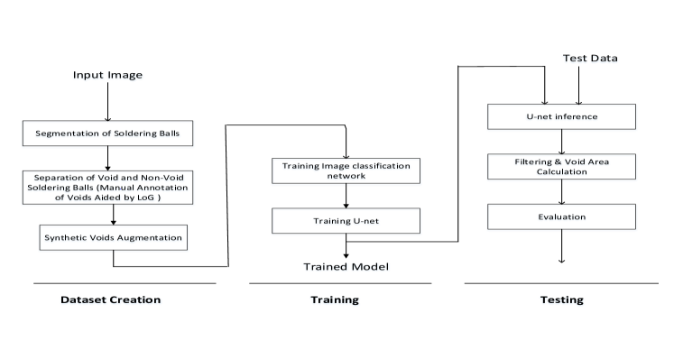
Figure 1: The Flowchart of Proposed Approach Consisting of Dataset Creation, Training and Testing

2.1 Dataset Creation

2.1.1 Segmentation of Soldering Balls

Given an input image,  Said et al. (2012) applied adaptive thresholding, circle detection and interpolating the occluded balls. The template matching approach is used to segment the occluding balls. The reference soldering ball is used to match all the locations in the occluded region. The location having the higher correlation is considered as the centre of the occluded soldering ball. In this paper, we follow the similar steps with some modifications. The steps in our proposed approach consists of slicing, otsu thresholding, circle fitting, filtering the false voids and interpolating the occluded balls. In this paper, we proposed the location based filtering using the information of un-occluded soldering balls. If the ball is missing in detection step then the distance between the neighbouring balls will be more. We interpolate the location of occluded one based on the distances of neighbouring soldering balls. The pseudo code of proposed algorithm is given in Algorithm 1.

Algorithm 1 Soldering Ball Extraction

1:Given an input image, divide it into non overlapping slices of size 300x400

2:For each slice, apply otsu thresholding

3:Rearrange the segmented slices in the corresponding position in the image to get the segmented image

4:Given the segmented image, find the circles and for each circle get the circle location and radius

5:Remove the circles (non-soldering balls) and interpolate the missing ones

6:Find the mode of the radius’s ($r_{mode}$), remove the circles (non-soldering balls) whose absolute difference between the $r_{mode}$ and the radius ($r$) is greater than $r_{thr}$. |$(r_{mode}-r)$|>$r_{thr}$ $r_{thr}$ = $r_{mode}$/sca. sca = 5 is selected heuristically that gives the best results.

7:Cluster the soldering balls based on the horizontal and vertical position. Each cluster will represent the group of soldering balls which are aligned in horizontal and vertical position

8:In case of ideal detection, the number of soldering balls in each cluster will be equal in horizontally and vertically. The horizontal and vertical between the soldering ball and neighbouring ones will be equal. The reference distance $d_{ref}$ is calculated for each soldering ball along horizontally and vertically.

9:In each cluster, find the distances between the neighbouring soldering balls. In case of missing ones, the distance (d) between the neighbouring ones will be more compared to the $d_{ref}$.

10:The location ($c_{x}$,$c_{y}$) of missing ones are interpolated using the neighbouring ones and using the $d_{ref}$.

11:After finding the ($c_{x}$,$c_{y}$), the reference (neighbour soldering balls) are used as template and a full search [-SR,SR]x[-SR,SR] is performed around the location ($c_{x}$,$c_{y}$). The location which gives the minimum error is considered as the optimal location.

2.1.2 Separation of Void and Non-Void Soldering Balls

Given the images of soldering balls, the void contours are generated through manual annotation. For this, LoG is applied at first to get the void contours. The LoG contours are classified into two categories, opened and closed. For closed contours, The region inside the contour represents the void and no manual labelling is required for these cases. Whereas, for opened contours, the contours are to be closed by manually labelling the most probable pixels that forms the closed contour. To do that, the input images, LoG contours are manually analysed by profiling the intensity values along horizontal and vertical around the void using ImageJ to find the most probable pixels that forms the closed contour. In case of overlapping contours, the contours are to be separated into individual ones. The manual process required is to separate the individual contours in case of overlapping contours. Given the input image and LoG mask, the overall manual process is to find the most probable pixels that can form the closed contour in case of open contours and separate the individual contours in case of overlapping contours. The voids with various strength usually appear in soldering balls, but the voids whose intensity is more than certain threshold $Thr_{min}$ are considered as real voids. For each contour, the average intensity of the pixels inside the contour is calculated representing the intensity of void ($I_{void}$). The average intensity of the pixels surrounding the void are calculated representing the background intensity ($I_{BG}$). Voids satisfying the condition ($I_{void}$ - $I_{BG}$) < $Thr_{min}$ are considered as invalid voids and these contours removed. After that, steps described in Algorithm 2 are applied to separate the soldering balls into void or non-void.

Algorithm 2 Separation of Void and Non-Void Soldering Balls

1:Given the contour image, check for existence of any closed contour that indicates the presence of void

2:if  any closed contour is found  then

3:     then classify it as void soldering ball

4:else Classify it as non-void soldering ball

2.1.3 Synthetic Voids Augmentation

It is widely known that, large dataset is the key to solve the problem using deep learning. Millions of images were needed to solve the image classification problem and became the backbone network to solve the various vision problems  He et al. (2015). Training the network using less number of samples can results in over-fitting that leads to poor accuracy. Recently, many novel approaches were proposed to solve the data and labelling problem for various complex computer vision tasks. As the millions of labelled samples may not be available in most of the cases, data augmentation, transfer learning  Tan et al. (2018), domain adaptation  Hoffman et al. (2017) and synthetic dataset creation became the vital approaches to improve the accuracy  Perez and Wang (2017). The simple photometric and geometric transformations like translation, rotation, scaling, noise etc., were used for data augmentation. Recently, GANs are more popular in generating synthetic samples that looks like real and are widely used in data augmentation, creation of adversarial examples and image translation. Unsupervised learning  Antoniou et al. (2017) techniques are used for learning features, if the labelled data is not available.

As it is difficult to get the void samples covering all the diversities (location, intensities and shape of voids, number of voids). Although data augmentation techniques are usually applied, but it easily leads to over-fitting and doesn’t increase the sample diversity for void segmentation. As from the manual annotation it is observed that number of non-void samples are more and the voids are of uniform intensity. There is a possibility to generate the synthetic voids with various intensities, sizes, count, locations and augment them on the non-void soldering balls that looks like real voids. This approach will create the more diverse samples and generalize the void detection that provides the better accuracy in real test time. The real void samples characteristics has to be considered in generating the synthetic voids so that the samples generated using synthetic domain should look as real. The characteristics to be considered in creating the synthetic voids are mentioned below.

Characteristics of the void to be considered in generated the dataset are

• Location of Voids: The voids can occur any location in soldering ball. The dataset should consists of voids in all possible locations

• Size of Voids: Voids can occur at any location. The dataset should consists of void with possible various sizes

• Number of Voids. The dataset should consists of with varying number of voids

• Brightness of Voids: The brightness of void can be of any intensity, some are less brighter and some are more. The dataset should consists of voids with various brightness

• Filtering between void and background: The intensity transition between ideal synthetic soldering ball and background is ideal. In practical, the transition is gradual. The low pass filter has to applied for the voids so that the edges of synthetic voids looks real. For generalization various low filters (amount of blur) has to be applied.

• The generated synthetic voids will be of uniform intensity with out any variations. To create, small intensity variations within the void, noise with different variances has to be added.

• Occurrences of multiple overlapping and non-overlapping voids are common, the dataset should consists of all possible combinations of multiple voids

Algorithm 3 Generation of Synthetic Dataset for Training U-net

1:The following steps [2-14] are repeated for $I_{max}$ number of times

2:Sample one of the non-void soldering ball

3:Sample a random number void count (VC) from the range [$VC_{min}$ $VC_{max}$] representing the number of voids

4:Sample the number of random values from the range [$VR_{min}$ $VR_{max}$] representing the void radius(VR) for each void

5:Sample the VC number of random values from the range [$VI_{min}$ $VI_{max}$] representing the void intensity(VI)

6:Sample the VC number of random values from the range [$VB_{min}$ $VB_{max}$] representing the void blur(VB)

7:Sample the VC number of random values from the range [$VN_{min}$ $VN_{max}$] representing the void noise (VN) variance

8:Sample the VC number of random values from the range [0 H] representing the void x-locations (VX) for each void

9:Sample the VC number of random values from the range [0 W] representing the void y-locations (VY) for each void

10:Generate the VC number of circular voids with the corresponding intensity VI, radius VR. The circular generation step consists of copying the intensity VI in all the pixel locations where the distance between the centre and the pixel location is less than radius VR.

11:In practical, voids will be appearing inside the soldering ball. In this approach, there is a possibility of voids crossing the boundary of soldering ball and is considered as invalid and shouldn’t be augmented. If any of the void crosses the boundary of soldering ball then remove the corresponding void.

12:Generate gaussian noise using the sampled noise variances VN and add to the generated circular voids.

13:Augmenting the voids to the soldering creates a sharp boundary between the void and background. In practical, the transition between the two void and background has to be smooth. So, we augment the each void on the sampled soldering ball blur the edges of voids with the sampled blur factors VB.

14:Add the void augmented soldering ball to the dataset

In this paper we considered all these mentioned factors in creating the diverse synthetic dataset. Regarding the shape of void, we assume that voids are circular. The factors considered here are void location (VL), void radius (VR), void brightness (VB), amount of void blur (VBL), void noise (VN) variance and number of voids or void count (VC). Given the minimum and maximum ranges of these values, we randomly pick one value for each of them and generate the void and augment on the soldering ball. Given the allowable minimum ($VR_{min}$) and maximum void radius ($VR_{max}$), minimum ($VC_{min}$) and maximum void count ($VC_{min}$), minimum ($VB_{max}$) and maximum ($VB_{max}$) void brightness, minimum ($VBL_{min}$) and maximum ($VBL_{max}$) blur factor, minimum ($VN_{min}$) and maximum ($VN_{max}$) noise variance, maximum images to be generated ($I_{max}$), image height (H) and width (W) and the images of non-void soldering balls, the procedure described in Algorithm 3 is applied to generate the synthetic dataset. The sample images of void augmented soldering balls and the corresponding void masks are shown in Fig. 2

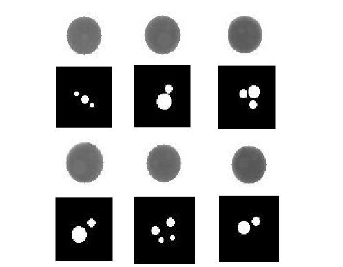
Figure 2: Sample Images of Artificial Voids Created on the Non-Void Soldering Balls

2.2 Training

2.2.1 Training Image Classification Network (Encoder)

The architecture of U-net is based on encoder and decoder networks. The encoder takes the input image and extracts the high level features. The decoder up-sample the extracted features to get the required output. There are skip between the encoder and decoder that copies the feature map of encoder output in each layer to the corresponding layer in decoder. At first, we construct the network for image classification to classify whether the image consists of void or not. After that, we remove the fully connected layer and add the decoder network to construct U-net. Weights for decoder are initialized randomly. The end to end U-net is trained for void segmentation. The reason to train the encoder network separately is to have the better initial weights during the training of U-net. The classification network and the corresponding network configuration is shown in Fig. 3 and Tab. 1. The input image size is 64x64 and is of gray level. During training, adam optimizer with initial learning rate (lr = $10^{-3}$) is used with batch size of 256.

Table 1: Encoder Network Configuration

Type	Filter size/stride(s)	Output size
Conv1	3x3/1	64x64x32
Pool1	2x2/1	32x32x32
Conv2	3x3/1	32x32x64
Pool2	2x2/1	16x16x64
Conv3	3x3/1	16x16x64
Pool3	2x2/1	8x8x64
Conv4	3x3/1	8x8x64
Pool4	2x2/1	4x4x64
Conv5	3x3/1	4x4x128
Pool5	2x2/1	2x2x128
Conv6	3x3/1	2x2x256
Pool6	2x2/1	1x1x256
Conv7	3x3/1	1x1x512

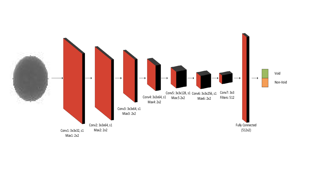
Figure 3: Encoder Trained with Fully Connected Layer for Void/Non-Void Binary Classification

2.2.2 Training U-net

After training image classification network, full connected layer is removed and the decoder network is added to the remaining network. The skip connections are added between encoder and decoder layers. The U-net architecture is shown in Fig.  4 and the corresponding configuration is shown in Tab.  2. The output mask is of same size as input size 64x64. Binary cross entropy is used as loss function. The value at each location indicates the probability belonging to void. Adam optimizer with learning rate (lr = $10^{-3}$) is used with batch size of 256.

Table 2: Decoder Network Configuration in U-net

Type	Filter size/stride(s)	Output size
Upsample1	2x2/1	2x2x512
Conv8	3x3/1	2x2x256
Concat(Upsample1, conv6)	-	2x2x512
Conv9	3x3/1	2x2x256
Upsample2	2x2/1	4x4x256
Conv10	3x3/1	4x4x128
Concat(Upsample2, conv5)	-	4x4x256
Conv11	3x3/1	4x4x128
Upsample3	2x2/1	8x8x128
Conv12	3x3/1	8x8x64
Concat(Upsample3, conv4)	-	8x8x128
Conv13	3x3/1	8x8x64
Upsample4	2x2/1	16x16x64
Conv14	3x3/1	16x16x64
Concat(Upsample4, conv3)	-	16x16x128
Conv15	3x3/1	16x16x64
Upsample5	2x2/1	32x32x64
Conv16	3x3/1	32x32x64
Concat(Upsample5, conv2)	-	32x32x128
Conv17	3x3/1	32x32x64
Upsample6	2x2/1	64x64x64
Conv18	3x3/1	64x64x32
Concat(Upsample6, conv1)	-	64x64x64
Conv19	3x3/1	64x64x32
Conv20	3x3/1	64x64x1

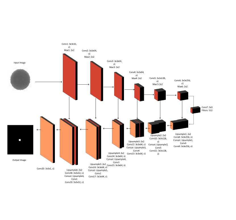
Figure 4: End to End Encoder-Decoder Network for Void Segmentation

2.3 Testing

For each segmented soldering ball in test set, the trained U-net is applied to get the probability map that indicates the presence of void at each location. The probability map is thresholded with threshold (0.5) to get the binary map. The value of 1 indicates the presence of void and for 0 it is the background.

2.3.1 Filtering and Void Area Calculation

After getting the void mask, connected component labelling is applied to separate the individual voids. Regions whose area is less than minimum area ($A_{min}$)are filtered out to eliminate the false predictions. The percentage of void area with respect to soldering ball is calculated as Percentage of Void (%) = (Area of void/Area of soldering ball) *100. Where, area of void is calculated by summing up number of pixels predicted as void. The area of soldering ball is calculated as the number of pixels inside the soldering ball.

3 Experimental Results

In this section we present the experimental results showing the capability of proposed synthetic data and void segmentation approach. The sample image of the dataset is shown in Fig. 5(a). The manually annotated and the proposed synthetic voids datasets are used to validate the proposed approach. The image resolution of the dataset is 64x64 where as the diameter of soldering ball is about 40x40. The search range (SR) used for soldering ball extraction is 5 pixels. $Thr_{min}$ used in separation of void and non-void soldering balls is 6. The parameters related to the synthetic data generation are $VC_{min}$ = 1 and $VC_{max}=4$, $VR_{min}$ = 2, $VR_{max}$ = 7, $VI_{min}$ = 6, $VI_{max}$ = 9, $VB_{min}$ = 2,$VB_{min}$ = 3, $VN_{min}$ = 1 $VN_{max}$ = 2. The minimum area to be considered as void is $A_{min}$ = 9.

To show the effectiveness of synthetic voids, the comparison results are classified according to the dataset used for training and testing. The following are the four comparisons used

1. Train on real voids data and test on real voids data ($Train\_Real\_Test\_Real$)
2. Train on synthetic voids data and test on real voids data ($Train\_Syn\_Test\_Real$)
3. Train on real and synthetic voids data and test on real voids data($Train\_Real\_Syn\_Test\_Real$)

The number of soldering balls in the real dataset consists of 3574. For $Train\_Real\_Test\_Real$, the manually annotated data is used for training and testing. For $Train\_Syn\_Test\_Real$, the same synthetic data is used for training and tested on real data. In $Train\_Real\_Syn\_Test\_Real$, real and synthetic data is used for training and tested on real data. The precision, recall and F1 score for all the cases is shown in Tab. 3. The detected voids for the sample full image is shown in the Fig. 5(b). The number on top of each soldering ball indicates the percentage of void with respect to the area of soldering ball.

Table 3: Precision, Recall and F1 Score Comparison

	Precision	Recall	F1 score
$Train\_Real\_Test\_Real$	0.92	0.73	0.82
$Train\_Syn\_Test\_Real$	0.84	0.77	0.80
$Train\_Real\_Syn\_Test\_Real$	0.95	0.76	0.84

In first case ($Train\_Real\_Test\_Real$), precision is more (false positives are less) and recall (false negatives are more). Due to less data, most of the voids are missed in detection resulting in more false negatives. In second case ($Train\_Syn\_Test\_Real$), the number of false positives are increased due to the domain differences between real and synthetic data, irregular voids in the real data. The number of missed detections are reduced due to use of synthetic data that covers most of the variations in the dataset. In third case ($Train\_Real\_Syn\_Test\_Real$), the number of false detections are reduced further, whereas the missed detections remained same. The reasonable F1 score can be obtained by using only proposed synthetic data compared to the one using real data. The network weights trained on synthetic data can be used as initial weights for training on real data with less number of real samples. With the help of synthetic data, less number of real samples are needed to get the better F1 score.

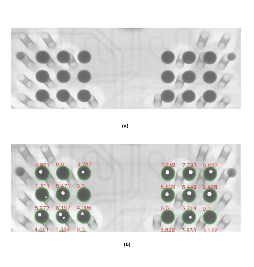
Figure 5: (a) Sample Test Image in the Dataset. (b) Detected Voids Overlaid in the Corresponding Test Image

4 Conclusion

The quality inspection of BGA by measuring the voids is vital for board yield issues. Various traditional approaches were proposed for void segmentation but lacks in scalability and provides less accuracy. In this paper, we applied U-net for void segmentation. In addition to that, we proposed an approach to generate the synthetic void dataset by considering the variations in real voids. The synthetic data improved the accuracy compared to the ones which is trained only using real data. The advantage of synthetic data is the data scalability and less number of real void samples are needed. The proposed system is scalable to various device types or products. There is a scope for further improvements in the future. In addition to the synthetic voids, synthetic soldering balls can be generated. In this paper, we assumed the void shape as circular, but in real the voids can be of any shape. Irregular shape voids can be generated and augmented for training. Improving the manual annotation can correctly evaluate the importance of synthetic data.

References

- Hillman et al. [2011] Dave Hillman, Dave Adams, Tim Pearson, Brad Williams, Brittany Petrick, Ross Wilcoxon, Rockwell Collins, Cedar Rapids, John Travis, Vineeth Bastin, and Nordson Dage. The last will and testament of the bga void. 2011.
- Said et al. [2012] Asaad F. Said, Bonnie L. Bennett, L. Karam, Alvin Kuok Lim Siah, Kevin Goodman, and J. S. Pettinato. Automated void detection in solder balls in the presence of vias and other artifacts. IEEE Transactions on Components, Packaging and Manufacturing Technology, 2:1890–1901, 2012.
- Peng and Nam [2012] Shao-Hu Peng and Hyun Do Nam. Void defect detection in ball grid array x-ray images using a new blob filter. Journal of Zhejiang University SCIENCE C, 13:840–849, 2012.
- Mouri et al. [2014] Motoaki Mouri, Yoichi Kato, Hiroshi Yasukawa, and Ichi Takumi. A study of using nonnegative matrix factorization to detect solder-voids from radiographic images of solder. 2014 IEEE 23rd International Symposium on Industrial Electronics (ISIE), pages 1074–1079, 2014.
- Said et al. [2010] Asaad F. Said, Bonnie L. Bennett, Lina J. Karam, and Jeffrey S. Pettinato. Robust automatic void detection in solder balls. 2010 IEEE International Conference on Acoustics, Speech and Signal Processing, pages 1650–1653, 2010.
- Ronneberger et al. [2015] Olaf Ronneberger, Philipp Fischer, and Thomas Brox. U-net: Convolutional networks for biomedical image segmentation. CoRR, abs/1505.04597, 2015. URL http://dblp.uni-trier.de/db/journals/corr/corr1505.html#RonnebergerFB15.
- He et al. [2017] Kaiming He, Georgia Gkioxari, Piotr Dollár, and Ross B. Girshick. Mask R-CNN. In IEEE International Conference on Computer Vision, ICCV 2017, Venice, Italy, October 22-29, 2017, pages 2980–2988, 2017.
- Shelhamer et al. [2017] Evan Shelhamer, Jonathan Long, and Trevor Darrell. Fully convolutional networks for semantic segmentation. IEEE Trans. Pattern Anal. Mach. Intell., 39(4):640–651, April 2017.
- Xue et al. [2018] Yuan Xue, Tao Xu, Han Zhang, L. Rodney Long, and Xiaolei Huang. Segan: Adversarial network with multi-scale L 1 loss for medical image segmentation. Neuroinformatics, 16(3-4):383–392, 2018.
- Zhou et al. [2018] Zongwei Zhou, Md Mahfuzur Rahman Siddiquee, Nima Tajbakhsh, and Jianming Liang. Unet++: A nested u-net architecture for medical image segmentation. In Deep Learning in Medical Image Analysis - and - Multimodal Learning for Clinical Decision Support - 4th International Workshop, 2018, and 8th International Workshop, ML-CDS 2018, Held in Conjunction with MICCAI 2018, Granada, Spain, September 20, 2018, Proceedings, pages 3–11, 2018.
- He et al. [2015] Kaiming He, Xiangyu Zhang, Shaoqing Ren, and Jian Sun. Deep residual learning for image recognition. CoRR, abs/1512.03385, 2015.
- Tan et al. [2018] Chuanqi Tan, Fuchun Sun, Tao Kong, Wenchang Zhang, Chao Yang, and Chunfang Liu. A survey on deep transfer learning. CoRR, abs/1808.01974, 2018.
- Hoffman et al. [2017] Judy Hoffman, Eric Tzeng, Taesung Park, Jun-Yan Zhu, Phillip Isola, Kate Saenko, Alexei A. Efros, and Trevor Darrell. Cycada: Cycle-consistent adversarial domain adaptation. CoRR, abs/1711.03213, 2017. URL http://arxiv.org/abs/1711.03213.
- Perez and Wang [2017] Luis Perez and Jason Wang. The effectiveness of data augmentation in image classification using deep learning. CoRR, abs/1712.04621, 2017. URL http://arxiv.org/abs/1712.04621.
- Antoniou et al. [2017] A. Antoniou, A. Storkey, and H. Edwards. Data Augmentation Generative Adversarial Networks. ArXiv e-prints, nov 2017.