The impact of cosmic rays on the sensitivity of JWST/NIRSpec

Abstract

The focal plane of the NIRSpec instrument on board the James Webb Space Telescope (JWST) is equipped with two Teledyne H2RG near-IR detectors, state-of-the-art HgCdTe sensors with excellent noise performance. Once JWST is in space, however, the noise level in NIRSpec exposures will be affected by the cosmic ray (CR) fluence at the JWST orbit and our ability to detect CR hits and to mitigate their effect. We have simulated the effect of CRs on NIRSpec detectors by injecting realistic CR events onto dark exposures that were recently acquired during the JWST cryo-vacuum test campaign undertaken at Johnson Space Flight Center. Here we present the method we have implemented to detect the hits in the exposure integration cubes, to reject the affected data points within our ramp-to-slope processing pipeline (the prototype of the NIRSpec official pipeline), and assess the performance of this method for different choices of the algorithm parameters. Using the optimal parameter set to reject CR hits from the data, we estimate that, for an exposure length of 1,000 s, the presence of CRs in space will lead to an increase of typically $\sim 7\%$ in the detector noise level with respect to the on-ground performance, and the corresponding decrease in the limiting sensitivity of the instrument, for the medium and high-spectral resolution modes.

1 Introduction

The James Webb Space Telescope (JWST) is widely seen as the scientific successor to the Hubble Space Telescope. Optimized for near and mid-IR observations, JWST is equipped with a 6.5 m diameter primary mirror and is passively cooled to less than 50 K (Gardner et al., 2009). Scheduled for launch in March 2021, the spacecraft will be placed in an orbit around the Sun–Earth Lagrange point L2. The JWST project is led by the National Aeronautics and Space Administration (NASA), with major contributions from the European Space Agency (ESA) and the Canadian Space Agency (CSA). The observatory will carry a suite of four science instruments, one of which is the Near Infrared Spectrograph (NIRSpec), developed by ESA with Airbus Defence and Space Germany as the prime contractor (Bagnasco et al., 2007; Birkmann et al., 2016). The primary goal of NIRSpec is to enable large spectroscopic surveys in the near-infrared with an emphasis on the study of the birth and assembly of galaxies.

To detect and characterize extremely faint astronomical objects, such as primordial galaxies, NIRSpec has to achieve very high sensitivity and thus its detector noise performance is crucial. For this reason, the NIRSpec focal plane is equipped with ultra low noise near-IR detectors: two Teledyne H2RG 2048$\times$2048 pixel, 5.3 $\mu$m-cutoff detectors, provided by NASA’s Goddard Space Flight Center (GSFC) (Beletic et al., 2008; Rauscher et al., 2014). The other two near-infrared science instruments onboard JWST (NIRCam and NIRISS) have similar detectors. The future ESA missions Euclid and Ariel will also be equipped with similar detectors and the next generation of the Teledyne HxRG family (H4RG) are planned for NASA’s Wide Field Infrared Survey Telescope (WFIRST).

As is often the case for IR detectors, both NIRSpec detectors (NRS1 and NRS2 hereafter), are read out non-destructively or “up-the-ramp”. An exposure comprises one or more ramps, also referred to as “integrations”. An integration consists of one or more “groups” (including the initial reset), and each group consists of one frame or the on-board average of multiple frames – for details, see Rauscher et al. (2007, 2010). For the full-frame mode that will be used to study faint astronomical objects, NIRSpec offers two readout options: the so-called traditional mode and the IRS² (Improved Reference Sampling and Subtraction) readout mode, developed by the NASA/GSFC team to minimize the presence of correlated noise caused by the detectors readout electronics (Rauscher et al., 2017). For each readout mode, two sampling patterns (with and without frame-averaging data) are available: NRS (averaging 4 frames per group) and NRSRAPID (1 frame per group) for traditional mode, and NRSIRS2 (averaging 5 frames per group) and NRSIRS2RAPID (1 frame per group) for IRS² mode – see also the JWST User Documentation.

Birkmann et al. (2018) have recently re-assessed the noise performance of NIRSpec detectors, using data acquired during cryogenic testing of the JWST OTIS element at Johnson Space Center in Summer 2017: 25 dark exposures in NRSRAPID mode with one integration of 88 groups each, and 30 exposures in NRSIRS2RAPID mode with one integration of 200 groups each. They conclude that the NIRSpec detector system meets its stringent noise requirement of 6 electrons total noise in a $\sim$1,000 s exposure. The question, however, is whether this performance will also be achieved once the instrument is in space and subjected to the intense CR flux expected for the L2 orbit. In this paper, we will address what type of performance degradation is to be expected due to the CR environment, and whether we have the tools to effectively minimize its detrimental effect on the NIRSpec performance.

In order to quantify the impact of CRs on NIRSpec observations, we have adopted a library of simulated CR events on IR detectors which was originally developed to test and optimize the JWST data processing pipeline (Robberto, 2010). We used the library to populate with CR hits the NIRSpec dark exposure data acquired during the OTIS test campaign. We then implemented a method to identify the hits in the integration ramps and remove them from the data cubes within the ’ramp-to-slopes’ part of the processing pipeline developed by the ESA NIRSpec team (which serves as template for the official NIRSpec pipeline developed by STScI). Our detection algorithm is based on the two-point difference method (Offenberg et al., 1999; Fixsen et al., 2000) and relies on thresholds tuned to achieve the best trade-off in terms of residual events and loss of effective integration time. We quantify the impact on the noise performance of the NIRSpec detectors from the CR bombardment expected for the JWST orbit by comparing the processed (CR-injected and removed) data with the original data.

The paper is organized as follows: the simulations of the CR events are presented in Sect. 2, while the CR detection and rejection algorithm is described in Sect. 3; the results in terms of residual noise levels for the different readout modes are summarized in Sect. 4 and discussed in Sect. 5.

2 Data and Simulated Cosmic Ray Events

2.1 Cosmic Ray library

Robberto (2010) presents a library of simulated cosmic ray events on JWST HgCdTe detectors. The cosmic rays are calculated for three different levels of solar activity, namely a) Solar minimum and Galactic maximum, b) Solar maximum and Galactic minimum, and c) Solar Flare, corresponding to three main space ionizing-radiation environments predicted by the CREME96 model (Tylka et al., 1997). The calculation takes into account the relative frequency of the most abundant nucleons: H, He, C, N, O, Fe, and their energy. Assuming a shielding of 100mil Al equivalent thickness, the model predicts a flux of 4.9, 1.8, and 3046 events ${\rm cm^{-2}~{}s^{-1}}$ respectively for the three levels of solar activity. The flux at Solar minimum is consistent with a typical particle background at L2 of 5 protons ${\rm cm^{-2}~{}s^{-1}}$ reported by the Planck and Gaia missions (Catalano et al., 2014; Crowley et al., 2016).

Cosmic rays impacting the detectors lose energy mostly through inelastic collisions with the bound electrons of the detector material. The detailed calculation of the energy loss is performed using SRIM (Stopping and Range of Ions in Matter, Ziegler et al., 2010) for different types of JWST detectors, characterized by the stoichiometric ratio of Hg vs. Cd (controlling the band gap of the HgCdTe alloy and therefore the long wavelength cutoff of the material), the material density (depending on the stoichiometric ratio) and thickness, assumed to be “optimally” tuned to be equal to the long wavelength cutoff of the material (5.3 $\mu$m in the case of the NIRSPEC detectors). The module TRIM (Transport of Ions in Matter) of the SRIM package allows the calculation of the 3D distribution of the ions in the material, together with the kinetic phenomena associated with the ion’s energy loss: target damage, sputtering, photon production and ionization, this last effect being the one of interest. Figure 1 shows an example of the TRIM calculations; the penetration of CRs into the material depends on their energy. The fractional energy loss is higher at low energy, as predicted by the classic Bethe-Bloch formula.

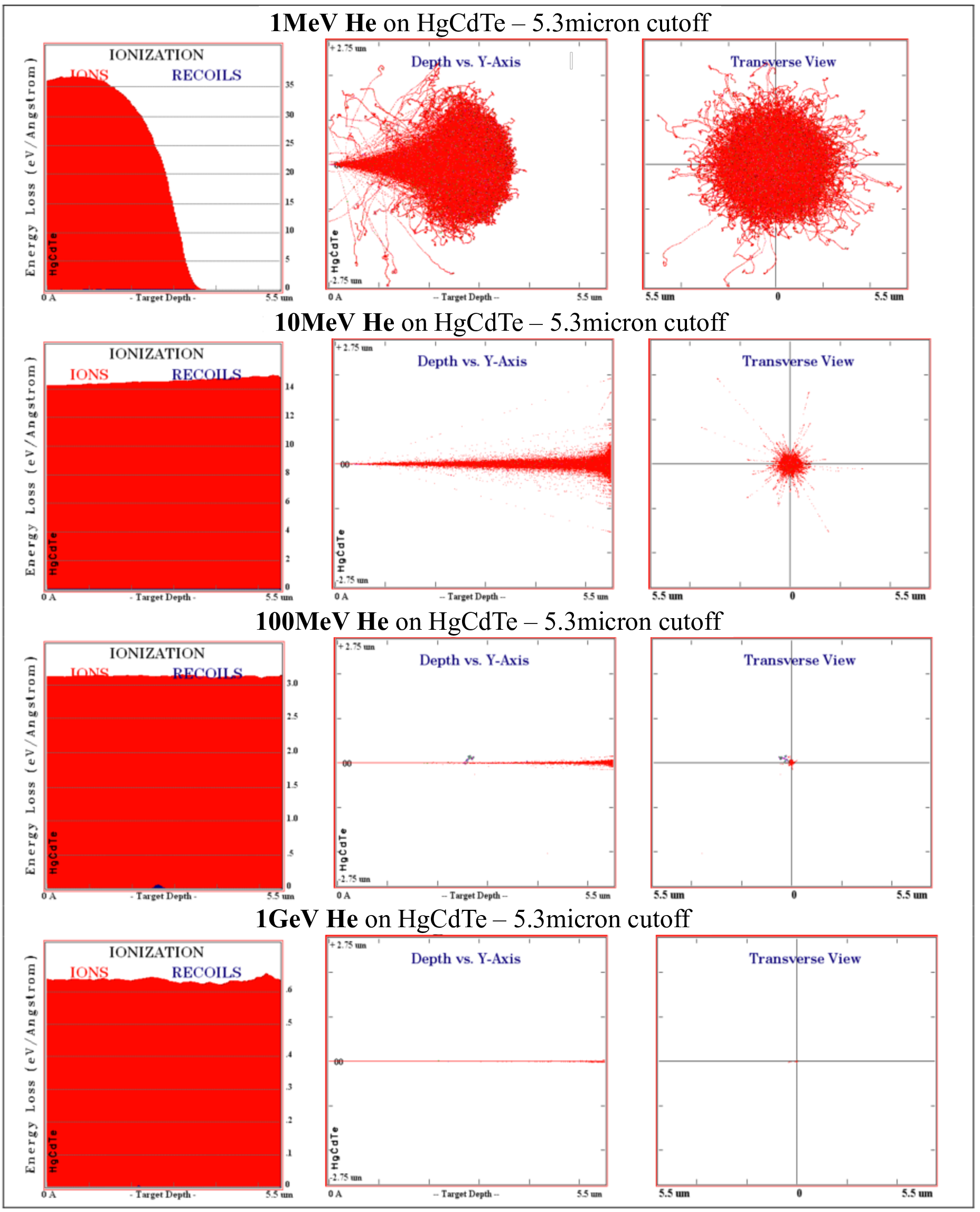
Figure 1: TRIM Results for He nuclei of different energy (from top to bottom: 1MeV, 10MeV, 100MeV, 1GeV) impacting on 5.3 $\mu{\rm m}$ HgCdTe. The left column shows the energy loss, the central column shows a longitudinal view with generated charges, the right column shows the transverse view of the generated charges.

The CR library is built performing Monte Carlo simulations of CRs generated by the CREME96 model that impact a random point within a pixel with a spatially isotropic distribution. The energy losses are determined following the CR through the pixels that are geometrically intersected, assuming to have a square 18 $\mu$m$\times 18~{}\mu$m surface and 5.3 $\mu$m thickness; grazing CRs can affect two or more pixels. For each event, the simulation calculates the electrons generated in a $21\times 21$ pixel region centered around the point of impact at pixel (10,10); this area is large enough to account for nearly tangential events and Inter Pixel Capacitance (IPC) coupling, i.e. the capacitive coupling arising between neighboring detector pixels in the source-follower CMOS design, via displacement currents flowing from the collection node (Moore et al., 2004).

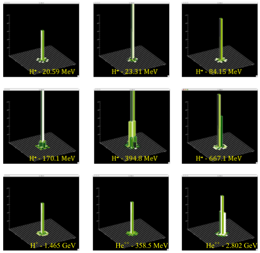
Figure 2: Simulated CR events on HgCdTe detectors for different energy levels of H and He nucleons, and including capacitive coupling.

The effect of IPC was taken into account by convolving each CR original image with a 5x5-IPC kernel $F(i,j)=\alpha^{d(i,j)}$, where $d$ is the distance from the central pixel and $F(0,0)$ is normalized to preserve the flux. The measured value of the coupling factor for our detectors varies from 0.003 to 0.007 across the four outputs. To be conservative, we assumed $\alpha=0.007$, resulting in the kernel shown in Table 1:

8.036E-07	1.519E-05	4.9E-05	1.519E-05	8.036E-07
1.519E-05	8.964E-04	0.007	8.964E-04	1.519E-05
4.9E-05	0.007	0.9681	0.007	4.9E-05
1.519E-05	8.964E-04	0.007	8.964E-04	1.519E-05
8.036E-07	1.519E-05	4.9E-05	1.519E-05	8.036E-07

Table 1: 5$\times$5-Kernel used to convolve the simulated CR-images and mimic the detector IPC

The library contains 30,000 CR events in the form of 21x21 postage-stamp arrays. In Figure 2 we present a few examples. For the analysis presented in this paper, we used the fluence level at Solar minimum and Galactic maximum, which is higher than the one for Solar maximum and Galactic minimum and therefore represents a conservative assumption for the typical (non-Solar flare) operating conditions of JWST.

2.2 Data processing

As mentioned before, we used 25 NRSRAPID dark exposures with 88 groups each (corresponding to $\sim$ 945 s integration time) and 30 NRSIRS2RAPID dark exposures of 200 groups each ($\sim$ 2,903 s integration time), acquired during OTIS testing at Johnson Space Center in Summer 2017.

CR events were injected into the dark exposures using scripts operating on the individual frames of an exposure ramp. The number of injected CR events per frame is determined by the integrated fluence (4.9 events ${\rm cm^{-2}~{}s^{-1}}$ assuming 100 mil Al equivalent thickness shielding), multiplied by the H2RG detector area, (i.e. 13.5895 cm²) and the frame readout time ($\sim$10.7 s for traditional readout and $\sim$14.6 s for IRS²), resulting in $\sim$ 710 and 970 CR hits per frame in Traditional and IRS² readout modes respectively. For each frame, the events are randomly drawn from the library and randomly placed (with a uniform distribution) across the detector arrays. The $21\times 21$ pixel large electron-rate ’postage stamp’ associated with each CR is converted into counts (using each detector’s average gain value) and added to the frame, resulting in a ’jump’ in the ramp of the affected pixels. If the maximum-value (i.e. saturation value) of the 16-bit analog-to-digital converter is reached, the ramp value is set to 65,535 from that sampling point onward. The CR-count injection onto the frame is a simple addition, with no attempt to account for the non-linear pixel response, which typically matters for count levels above $\sim$ 50,000 counts, or other effects such as, e.g. persistence (see also the discussion in Sect. 5). CRs were only injected into the light sensitive pixels (i.e. the central 2040 x 2040 pixel region of each detector), but not the 4-pixel wide ’frame’ of reference pixels.

Throughout the duration of an exposure, the number of pixels affected by a CR hit increases with the integration time: at the end of a traditional-mode 88-groups integration, $\sim$ 15% of pixels have been affected by at least one hit, while at the end of a IRS²-mode 200-groups integration $\sim$ 40% of pixels have been affected. Fig. 3 shows the histogram of the injected events for the dark exposures of NRS1. The distribution of charge injected into individual pixels steeply increases at low count levels. The event histograms for NRS2 look very similar, and are not shown.

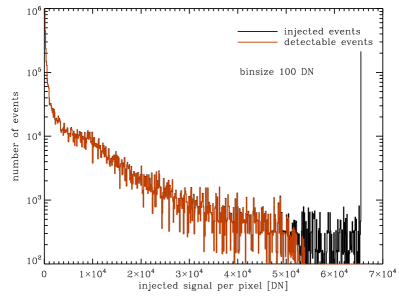
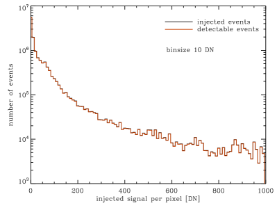
Figure 3: Histogram of the injected events for the NRS1 exposures. Complete histogram with 100 DN bin size is on the left, a more detailed view for the low levels at the right. The black curve corresponds to all injected events, whereas the red curve is for detectable events only. Events above $\sim$55,000 counts can never be detected by the pipeline, because when added to the bias level they exceed the range of the analog to digital converter, and are therefore flagged as saturated.

All the exposures were processed with the ESA NIRSpec ramp-to-slope pipeline that performs the following basic data reduction steps.

• Saturation detection and flagging: each pixel value in each group is compared to the pixels’ saturation threshold stored in a reference file, and flagged as saturated if it exceeds the threshold. Data flagged as saturated are not used when determining the count rate.

• Master bias subtraction: the master bias, i.e. the detector frame readout at zero seconds, derived from averaging the first frame of many dark exposures, is subtracted from each group, pixel-by-pixel.

• Reference pixel subtraction: for Traditional readout, the four rows of reference pixels at the top and bottom of the detector (eight rows in total) are used to determine the pedestal for each group and output. The average pedestal is subtracted from all pixels in a given output in each group. Finally, a correction along the slow readout direction is performed using the four columns of reference pixels to the left and right and a running windowed average. For IRS² readout, the interleaved reference pixels and reference output are subtracted from all pixels using a statistically optimized set of frequency dependent weights to better correct for $1/f$-noise and correlation in the detector data, as described in Rauscher et al. (2017).

• Dark subtraction: the reference dark cube is subtracted from each group, pixel-by-pixel.

• Count rate estimation, including jump detection and CR rejection: in this step, the count rate per pixel is estimated using all unsaturated groups in the ramp, and ’jumps’ (e.g. due to CR hits) are detected and rejected by estimating the slope of individual ramp segments on either side of the affected frame. More details on this step are provided in the next section.

3 Detection and Rejection of CR events

To illustrate the slope estimation algorithm used by the ESA pipeline, we assume an integration with $n$ unsaturated groups with $m$ frames each (for NIRSpec $m=1,4,$ or $5$, depending on the readout mode and pattern). For a given pixel, the measured signal at each group $i=1\ldots n$ is $s_{i}$ (in DN, i.e. Digital Number). The count rate $b$ in electrons per second for that pixel is then

$$b=\frac{g}{t_{g}}\sum_{i=1}^{n}a_{i}s_{i},$$ (1)

where $g$ is the conversion gain in electrons/DN for the given pixel, $t_{g}$ is the group time in seconds, and $a_{i}$ are pre-computed and normalized weights (their sum normalized to 1). The weights depend on the read noise $\sigma$, the estimated signal $s$, and the number of groups in an integration $n$. Details on how the weights are calculated are given in Fixsen et al. (2000), who show that optimally weighting is needed to efficiently deal with different regimes of signal-to-noise. In the low signal to noise limit where $b\times t_{g}\ll\sigma^{2}$ each group is weighted the same. This is equivalent to uniform weighting and a linear fit to the data. In the high signal to noise regime where $b\times t_{g}\gg\sigma^{2}$ the full weight is on the endpoints $s_{1}$ and $s_{n}$ and the data in between are basically ignored, optimizing effective integration time – see also Robberto (2014) on the issue of generalized least square in non-destructive readouts.

CR hits on the pixel during the integration will deposit additional charge which will lead to a jump or discontinuity in the ramp and skew the estimated slope if not corrected for. If an integration has enough groups ($n\geq 3$), one can evaluate the $(n-1)$ pair-wise differences (or correlated double sample, CDS) in order to look for outliers:

$$d_{i=1\ldots n-1}=s_{i+1}-s_{i}.$$ (2)

If only two data points are available ($n=2$), no outliers detection can be performed as there is only one pair, and the signal is directly calculated using equation 1. A first robust estimate of the average difference / signal between groups is obtained by averaging the differences after removing the most extreme values:

$$d_{avg}=\left\{\begin{array}[]{ll}\frac{1}{n-2}\left((\sum_{i=1}^{n-1}d_{i})-d_{max}\right)&\mathrm{for}\;n=3\\ \frac{1}{n-3}\left((\sum_{i=1}^{n-1}d_{i})-(d_{max}+d_{min})\right)&\mathrm{for}\;n>3\\ \end{array}\right\},$$ (3)

where $d_{max}$ and $d_{min}$ are the maximum and minimum of all the differences $d_{i}$, respectively. This is done to remove the contribution of potential outliers from the average. The expected variance of the two-point differences $d_{i}$ is then

$$\sigma_{cds}^{2}=\frac{2}{m}\sigma_{read}^{2}+g\left(1-\frac{m^{2}-1}{3m^{2}}\right)d_{avg}.$$ (4)

In order to detect significant outliers from this, we calculate the deviations from the mean difference and the maximum absolute outlier

$$\delta_{j}=max(|\delta_{i=1\ldots n-1}|)=max(|d_{i=1\ldots n-1}-d_{avg}|)$$ (5)

and store the position of the maximum absolute difference as $j$. $\delta_{j}$ is then compared to the expected noise times a threshold scaling factor $c_{th}$ and flagged as an outlier if the noise threshold is met or exceeded:

$$|\delta_{j}|\geq c_{th}\sigma_{cds}.$$ (6)

If the worst offender exceeds the set threshold, the integration will be split into two segments at difference $j$, and the count rate $b_{1}$ and $b_{2}$ of those segments will be determined independently:

$$\begin{array}[]{ll}b_{1}&=\frac{g}{t_{g}}\sum_{i=1}^{j}a_{i}s_{i},\\ b_{2}&=\frac{g}{t_{g}}\sum_{i=j+1}^{n}a_{i}s_{i}.\\ \end{array}$$ (7)

The ramp segments have $n_{1}=j$ and $n_{2}=n-j$ data points, respectively. These numbers are used to determine the optimal weights $w_{1}$ and $w_{2}$ for combining the ramp segments count rates according to Offenberg et al. (1999):

$$\begin{array}[]{ll}w_{1}&=(n_{1}-1)n_{1}(n_{1}+1),\\ w_{2}&=(n_{2}-1)n_{2}(n_{2}+1),\\ \end{array}$$ (8)

with the final / combined count rate being $b_{f}$:

$$b_{f}=\frac{w_{1}b_{1}+w_{2}b_{2}}{w_{1}+w_{2}}.$$ (9)

The above approach effectively mitigates one significant (i.e. detected) outlier in an integration. To be able to detect multiple events, the above (equations 2 through 9) are recursively repeated for the ramp segments $i=1\ldots j$ and $i=j+1\ldots n$, so that outliers can be detected in these sub-ramps as well. This recursive process is stopped when either no outliers are detected in the sub-ramp anymore or the number of groups per (sub-)ramp becomes $n\leq 2$. The points in time (positions in the ramp) where these outliers are detected can be stored to be able to compare the masks of simulated injected CR events with the ones detected by the pipeline.

The process outlined above is performed for each pixel in the detector individually. However, it is expected that typical CR events will affect a group of adjacent pixels rather than a single one mainly because of the coupling due the IPC, but also because of the intrinsic shape of the CR footprint. Therefore, the pipeline offers the possibility to identify neighbors of (clusters of) pixels and perform a second detection and rejection cycle with a different threshold on those pixels.

We investigated two options for selecting neighbors: i) directly adjacent pixels of any pixel that has a CR event of at least a certain magnitude, or ii) neighbors adjacent to a cluster of pixels with detections at the same group. A cluster consists of two or more pixels that are directly adjacent, i.e. neighbor at the top, bottom, left or right. Pixels that are located diagonally across are not considered neighbors nor members of the same cluster, as illustrated in Fig.  10.

It is expected that most CR events of significant magnitude will impact more than one pixel, therefore only considering neighbors around clusters of two or more adjacent pixels for a second pass might be sufficient. Also, both NIRSpec detectors have a small population of pixels exhibiting Random Telegraph Noise (RTN), a phenomenon in which a pixel counts transition rapidly, and almost ‘digitally’, between two levels (Bacon et al., 2004; Rauscher et al., 2004). Our approach of flagging only cluster neighbors therefore has the advantage of limiting the impact of RTN pixels affected on their neighbors, i.e. not unnecessarily breaking up ramps. On the other hand, the cluster approach potentially leads to issues caused by the effects of IPC, because the neighbors of single pixel events will not be flagged, regardless of how strong the event was. Therefore, the pipeline also allows the flagging of neighbors that are next to individual pixels that have been flagged, as long as the jump in the latter is of sufficient magnitude. The default jump threshold was selected to be 200 DN, which is large enough to exclude most RTN pixels.

The second detection pass on single-pixel neighbors is then performed with a threshold $c_{nb}$ using equation 6, with $c_{nb}$ replacing $c_{th}$, and only considering the two-point differences where the parent CR of the adjacent cluster/pixel took place (there can be more than one event in a ramp). To have any effect $c_{nb}$ has to be lower than $c_{th}$ (otherwise the event would have been found in the first pass already) and it can be as low as zero, which means that the ramps of the neighbors will always be broken into sub-ramps at the position of the parent event (i.e. the condition in equation 6 is always fulfilled). The two or more sub-ramps are then individually processed and combined to a final count rate using the weighting scheme outlined in Sect. 2.2.

We evaluated the efficiency of detecting CR hits for different values of $c_{th}$ and $c_{nb}$ as described in the Appendix.

4 Results

4.1 Traditional readout

In order to evaluate the impact of CR hits on the NIRSpec sensitivity, we evaluated the typical noise in dark exposures by first calculating the standard deviation per pixel across all 25 processed exposures, and then deriving the median value across all $2040^{2}$ pixels. This was done for both the original darks and the CR-injected darks, the latter being processed for different combinations of $c_{th}$ and $c_{nb}$. The total noise in e^- was then calculated by multiplying the median standard deviation with the effective integration time $t_{eff}=\left(n-1\right)t_{g}$ and the conversion gain (e^-/DN). The results are presented in Figures 4 and 5. The lowest total noise is achieved for threshold multiplier values of $c_{th}\gtrsim 4$ for all neighbor detection thresholds. The total noise degrades rapidly with lower thresholds. Higher thresholds have less impact on the achieved noise, and are in fact preferred for the original data without the added simulated CR events, although the total noise curve is basically flat for $c_{th}>4$.

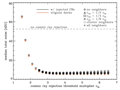
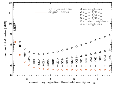
Figure 4: Median total noise for NRS1 for the 25 dark exposures with (black symbols) and without (red symbols) simulated CR events. The dashed black line in the left panel shows the noise with no CR rejection at all ($c_{th}=\infty$). The right panel gives a more detailed view of the lower total noise range.

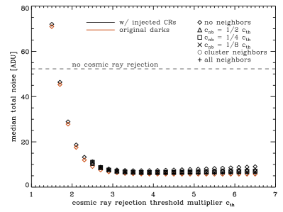
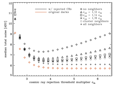
Figure 5: Median total noise for NRS2 for the 25 dark exposures with (black symbols) and without (red symbols) simulated CR events. The dashed black line in the right panel shows the noise with no CR rejection at all ($c_{th}=\infty$). The right panel gives a more detailed view of the lower total noise range.

The reason for the observed behavior can be interpreted as follows: as apparent from the plots in Appendix A, a low detection threshold $c_{th}$ will lead to many “false positive” detections. Due to the symmetric nature (both positive and negative outliers are flagged) of the detection algorithm, this should not introduce a bias to the estimated slope. However, it will have a negative effect on the achieved signal-to-noise, because integrations are unnecessarily broken up into many shorter sub-ramps, which is particularly detrimental in the low signal-to-noise regime (e.g. darks), where the read noise dominates. At higher thresholds, a smaller and smaller fraction of affected pixels is actually detected, leading eventually to an increase in total noise.

It is also evident that enabling a secondary pass on neighbors of detected pixel clusters with a lower threshold reduces the total noise, as long as the initial threshold $c_{th}$ is not too low. In Table 2 we list the best parameter values (i.e. yielding the lowest noise) for each tested method of neighbor detection in the two detectors.

$c_{nb}$	NRS1		NRS2
	$c_{th}$	noise [e-]	$c_{th}$	noise [e-]
$\infty$ (no neighbors)	3.5	7.038	3.7	8.294
$1/2\times c_{th}$	3.7	6.463	3.9	7.589
$1/4\times c_{th}$	3.9	6.261	3.9	7.343
$1/8\times c_{th}$	3.9	6.184	4.1	7.258
$0$ (all cluster neighbors)	3.9	6.125	4.1	7.186
$0$ (all neighbors)	4.9	5.910	5.1	6.914
original data (no neighbors)	5.3	5.568	5.7	6.487

Table 2: Best parameters for CR detection threshold multiplier $c_{th}$ and the associated total noise for different values of $c_{nb}$ for the two NIRSpec detectors. The last row gives the total noise measured for the original dark data without simulated CRs added.

The lowest total noise is achieved using a second CR rejection iteration on all neighbors (i.e. with a threshold of $c_{nb}=0$), including neighbors of single pixel events that are marked as severe. That means that for these neighbors, the ramps are broken at the same position as the parent cluster/pixel, regardless of the two-point difference. Given the steep rise of total noise towards lower values of $c_{th}$ and the little impact of using higher and higher threshold values, in particular when flagging all neighbors (see Figures 4 and 5), the best combination of threshold values are $c_{th}=5.0$ and $c_{nb}=0$ with single pixel neighbor flagging, for both detectors.

Fig. 6 shows the noise distributions for the original data and the data with injected CRs, each with and without second pass neighbor processing. The histograms demonstrate that a significant tail of pixels with higher noise remains in the processed darks, unless neighbors are also considered. This is reflected in the median noise values; compared to the original data without injected CRs, the total noise increases by $\sim$6 % for NRS1 and $\sim$7 % for NRS2, respectively, when a second pass on neighbors is performed, while increasing to $\sim$26 % (NRS1) and 28 % (NRS2) higher total noise with no second pass. The visual appearance of the same count-rate image processed with the different options for considering neighbors, shown in Fig. 12 of the Appendix, also demonstrates that the ‘all-neighbors’ choice delivers the cleanest results.

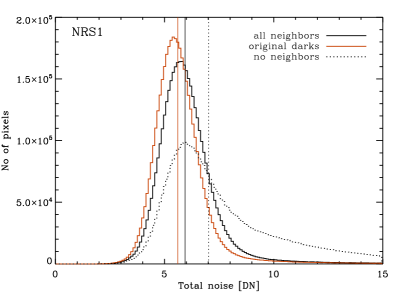
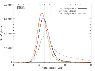
Figure 6: Total noise histograms for NRS1 (left) and NRS2 (right). Red lines are for the original dark data with no added cosmic ray events, solid black lines for data with cosmic rays added and rejected with the ’all neighbors’ method, and dotted black lines when not performing a second pass on the neighbors. In all cases, the histogram for the best rejection threshold $c_{th}$ is shown. The vertical lines denote the median total noise as presented in Table 2.

To study the effects of CRs on frame-averaged data, we used the same traditional darks taken at OTIS, with and without injected cosmic ray events, and frame-averaged them as would be done onboard. We repeated the analysis described above, focusing on three test cases: i ) $c_{th}=[1.5\ldots 6.5]$ in steps of $0.2$ with no second pass on neighbors (also for original data without simulated CRs); ii) $c_{th}=[2.5\ldots 6.5]$ in steps of $0.2$ with cluster neighbor detection enabled at $c_{nb}=0$; iii) $c_{th}=[2.5\ldots 6.5]$ in steps of $0.2$ with all pixel neighbor detection enabled at $c_{nb}=0$, as long as the parent event causes a jump of at least 200 DN. The total noise results for the frame-averaged data is presented in Figure 7, and the best value of $c_{th}$ for each case is given in table 3 below.

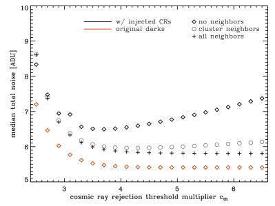
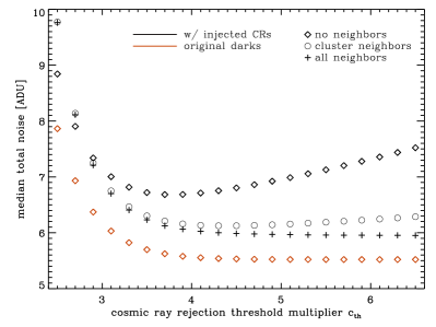
Figure 7: Median total noise for NRS1 (left) and NRS2 (right) for the 25 frame-averaged dark exposures with (black symbols) and without (red symbols) simulated CR events.

$c_{nb}$	NRS1		NRS2
	$c_{th}$	noise [e-]	$c_{th}$	noise [e-]
$\infty$ (no neighbors)	3.7	6.465	3.7	7.590
$0$ (all cluster neighbors)	4.3	5.933	4.3	6.956
$0$ (all neighbors)	5.9	5.779	6.5	6.759
original data (no neighbors)	5.3	5.383	5.7	6.270

Table 3: Best parameters for CR detection threshold multiplier $c_{th}$ and the associated total noise for different values of $c_{nb}$ for the two NIRSpec detectors for frame-averaged data. The last row gives the total noise measured for the original (frame-averaged) dark data without simulated CRs added.

The results are in line with those for the non-frame-averaged data, with a second pass on all neighbors – including those adjacent to severe single pixel events – being best. The optimal value of $c_{th}$ is higher than for the non-frame-averaged case. For the best method with all neighbors flagged, we recommend $c_{th}=6.0$ for frame-averaged data. The increase in total noise over the data without simulated cosmic rays is $\sim$7 % for NRS1 and 8 % for NRS2, respectively, slightly larger than for the non-frame-averaged data. This can be attributed to the ’dilution’ of CR events in the frame-averaged data, making detection more challenging, and the fact that more data is lost due to a CR event when using frame-averaging (longer effective groups, and one CR can lead to two jumps in the ramp). Without a second pass on neighbors the noise increase is $\sim$20 % (NRS1) and $\sim$21 % (NRS2).

Note that although the total noise values on the number of accumulated electrons (in e^-), for the frame averaged data, are slightly smaller than those for the non-averaged ones (cf. Table 2 and Table 3), the total noise on the associated electron-rate (in e${}^{-}/s$) are slightly larger, because the effective integration time, $t_{eff}$, decreases as $t_{g}$ increases with the number of averaged frames.

4.2 IRS² readout

Using the 30 dark exposures that were taken in IRS² readout mode, we processed both the original data and the data with cosmic rays added. The dark exposures taken in IRS² mode are longer than those in traditional readout mode (200 groups, corresponding to $\sim$3,000 seconds). Therefore, we processed both the full length exposures and only the first 65 groups of each integration, resulting in two data sets. The shorter integrations (65 groups, $\sim$1,000 s) are comparable in length to the traditional data.

The processing of IRS² readout mode data is more time intensive, therefore we focused on three methods for the cosmic ray rejection - no neighbors, neighbors of clusters, and all neighbors - and used a coarser sampling of rejection threshold values $c_{th}$. The determination of total noise was achieved in the same way as outlined in section 4.1 for the traditional data. The results for both detectors are shown in Figures 8 and 9 for the short (65 groups) and full (200 groups) integrations, respectively.

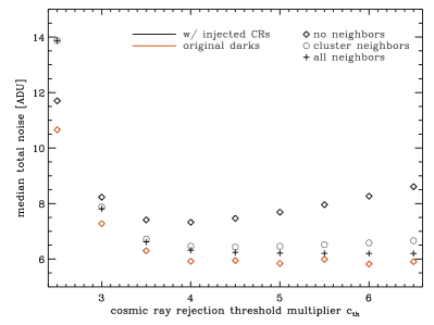
Figure 8: Median total noise for NRS1 (left) and NRS2 (right) for the 30 dark exposures (NRSIRS2RAPID mode) with (black symbols) and without (red symbols) simulated CR events, processed up to 65 groups ($\sim$1,000 s integration time per exposure).

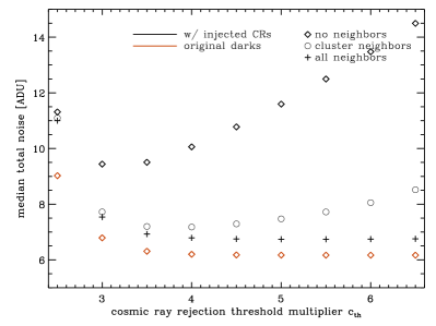
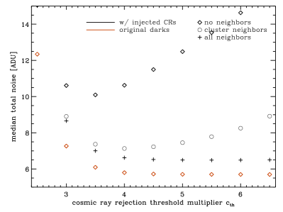
Figure 9: Median total noise for NRS1 (left) and NRS2 (right) for the 30 dark exposures with (black symbols) and without (red symbols) simulated CR events, for the full length integrations (200 groups, $\sim$3,000 s).

The results are in line with those for the traditional data, with flagging of all neighbors yielding the lowest noise for CR-affected data. Table 4 lists the best values for each tested method, for both the short and full IRS² integrations.

	65 groups				200 groups
$c_{nb}$	NRS1		NRS2		NRS1		NRS2
	$c_{th}$	noise	$c_{th}$	noise	$c_{th}$	noise	$c_{th}$	noise
$\infty$ (no neighbors)	3.5	6.343	4.0	8.319	3.0	9.397	3.5	11.463
$0$ (all cluster neighbors)	4.0	5.610	4.5	7.317	4.0	7.146	4.0	8.099
$0$ (all neighbors)	4.5	5.452	6.0	7.045	5.5	6.709	5.5	7.369
original data (no neighbors)	6.0	5.150	6.0	6.614	6.5	6.141	6.5	6.471

Table 4: Best parameters for CR detection threshold multiplier $c_{th}$ and the associated total noise (in e^-) for different values of $c_{nb}$ for the two NIRSpec detectors in IRS² readout mode. Results are for two different integration times of $\sim$1,000 s (65 groups) and $\sim$3,000 s (200 groups). The last row gives the total noise measured for the original dark data without simulated CRs added.

For the short integrations, the increase in total noise with respect to the original data is comparable to the results for the traditional readout mode. For the best rejection method (two passes with all neighbors flagged), the increase in noise is $\sim$6 % for NRS1 and $\sim$6.5 % for NRS2, respectively. For the single-pass method (no neighbors), the noise increase is 23 % (NRS1) and 26 % (NRS2) compared to the original data.

For the full (200 groups) integrations the increase in noise is significantly higher, with $\sim$9 % for NRS1 and $\sim$13 % for NRS2 when using the best (all neighbors) rejection. For the single-pass method, the increase is even more pronounced, at 53 % (NRS1) and 77 % (NRS2).

5 Discussion and conclusion

The aim of this work was to assess the impact of the CR bombardment expected at L2 on the noise performance of the (flight) NIRSpec detectors, and to investigate CR rejection algorithms based on the two-point difference method (Offenberg et al., 1999; Fixsen et al., 2000) to detect the CR-induced jump, and then split the signal ramp at the impacted frame to perform the ramp fitting on the separate segments.

Anderson & Gordon (2011) used simulations of JWST-like integration ramps to study three methods to detect CR hits and concluded that the two-point difference is the most effective in the shot-noise limited regime and the best trade-off in terms of effectiveness and speed for read-noise limited exposures. Additionally, the uncertainties associated with this correction method are quasi-Gaussian, which simplifies the process of choosing a rejection threshold. Nevertheless, because of the presence of significant inter-pixel signal coupling due to IPC in these detectors and because the CR signature often involves more than one pixel, applying this approach only to the pixel(s) where the hit is initially detected leads to considerably worse total noise for our detectors compared with ground-data: up to $\sim$ 30% of the noise level for integration lengths of 1,000 s and more than $\sim$ 75% for integrations of 3,000 s.

Our analysis shows that significantly better noise performance can be achieved with a second pass which addresses the direct neighbors of CR-affected pixels and applies the same ramp-splitting to them. This is in line with the results by Fadeyev et al. (2006) who also found that interpixel correlation substantially increases the footprint of CR impacts and treated neighboring pixels with a second pass in their pipeline for NICMOS data reduction. By including neighboring pixels in our CR mitigation approach, we achieve noise levels that are only slightly elevated compared to ground performances: by about 7% for 1,000 s integrations and 15% for 3,000 s.

The increase in noise is mainly due to two effects. Some CRs will cause saturation of the pixel so the slope can only be estimated from data before the hit occurred, yielding a reduction in effective integration time. Even if the cosmic ray event does not result in saturation, the ramp needs to be split. While the full data loss is low (typically one group time, up to two group times for frame-averaged data per event), the two ramp segments need to be fit individually, and the variance of the combined slopes is higher than that of a single, uninterrupted ramp. The detrimental effect of cosmic rays is more pronounced for longer integrations, because more data can be lost to early saturation due to a CR hit, and also more pixels are affected by a CR, i.e. have their integration broken into two or more segments.

Besides the impact on the noise statistics of the detectors presented here, CRs can also lead to systematic effects and bias the measurements in more subtle ways that are not addressed by our analysis. In first instance, the choice of threshold value impacts the fraction of CR-affected pixels that will go undetected, and these will inevitably bias the overall signal distribution to a higher value. For each of the CR affected pixels, in every exposure, we computed the difference in count rate between the original data and the CR-injected data processed with a range of $c_{th}$ values (all-neighbors method); the mean excess signal (of all CR-affected pixels, excluding hot pixels) increases approximately linearly with the threshold, for $c_{th}$ in range 2.5$-$6.5. This bias (i.e. offset of the mean from zero) is, however, small compared to the count-rate variations, less than 10% of the RMS of the difference distribution, for $c_{th}=6.5$.

Near-IR detectors exhibit the effect of persistence (Regan & Bergeron, 2018). The physical process that causes the persistence has been ascribed to charge ’traps’, i.e. defects in the semiconductor material that capture charge during the stimulus image and then slowly release it over time. Therefore the persistent signal from strong CR hits, corresponding to a count of more than $\sim$ 50,000 electrons, can pollute subsequent images as well as affect the linearity of the pixel response after the hit, as some of the charge-traps “leak” additional spurious signal. Furthermore, following such a strong CR hit, the pixel will be operating at a higher count level, closer to its inherent non-linear regime, where the non-linearity correction is applied by the ramp-to-slop pipeline. This may also impact somewhat the total noise figure, as the accuracy of the flux estimate is affected by the uncertainties of the linearity correction. With the CR fluence assumed in this work, in a 1,000 second integration, fewer than 0.3% of the pixels (about 10,000) are affected by an event that introduces more than 50,000 electrons. For specialized programs aiming to minimize potential systematic errors, one option may simply be to flag and discard disturbed pixels; in this context, the method presented here allows a more comprehensive flagging of affected pixels.

We also note that, in our simulations, CRs were only injected into the light sensitive pixels (central 2040 x 2040 region of the detector) and not the four pixel wide ’frame’ of reference pixels (or the interleaved reference pixels in case of the IRS² readout data). Indeed, the simulated events are modeled for charge deposited into an active layer of HgCdTe, and not for effects on the underlying read out integrated circuit (ROIC). This is justified by detector data from the Hubble Space Telescope Wide Field Camera 3 which is equipped with a previous generation of Teledyne near-IR detectors (HAWAII-1R). Those data indicate that CRs do not appear to affect significantly the reference pixels (Ben Sunnquist, personal communication).

In conclusion, our analysis has allowed us to develop an effective way to deal with the CR bombardment expected for NIRSpec detectors in flight, and to show that with a tailored rejection algorithm, the CR hits will cause only a small deterioration of the detectors’ total noise level, with an increase of $\sim$ 7%, for the bench mark 1,000 s exposures. This corresponds to a 7% decrease in the limiting sensitivity of the instrument for the medium and high-spectral resolution modes ($R=1000$ and $R=2700$) that, for faint targets, are fully detector-noise limited; for the low-spectral resolution configurations ($R=100$) that are not typically detector noise limited (because background noise is a significant contributor), the impact of the noise increase is lower, 3-4% depending on wavelength. Such small decreases in sensitivity are not a concern for the achievement of the NIRSpec scientific goals.

Appendix A Cosmic Ray Detection Efficiency

As described in Sect. 3 our pipeline offers the possibility to perform a second pass of outliers detection for pixels at a lower threshold for the neighbors of pixels that had a detected CR in the first pass, with two options for selecting neighbors: i) directly adjacent pixels of any pixel that has a CR event of at least a certain magnitude, or ii) neighbors have to be adjacent to a cluster of pixels with detections at the same group. A cluster consists of two or more pixels that are directly adjacent, i.e. neighbor at the top, bottom, left or right, as shown in Fig. 10.

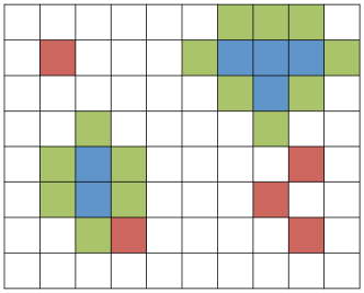
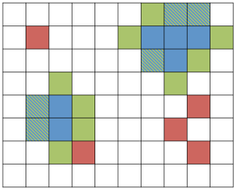
Figure 10: Schematic of a grid of 10 by 8 pixels (white squares) with some cosmic hits / outliers detected using a threshold $c_{th}$ (left). Outliers can occur isolated (red) or in clusters (blue). The direct neighbors of cluster pixels are marked in green. These pixels can then be given more scrutiny in a second detection pass that uses a lower detection threshold $c_{nb}$. In this example five additional pixels were found with this lower threshold, marked with blue/green stripes (right).

To asses the efficiency of CR detections by the pre-processing pipeline, the detected events were recorded and compared to the injected simulated events that are detectable, i.e. occur after the first group is read and do not lead to saturation. The number of pixels with detected events per frame for both detectors as a function of detection thresholds $c_{th}$ and $c_{nb}$ is shown in Figure 11.

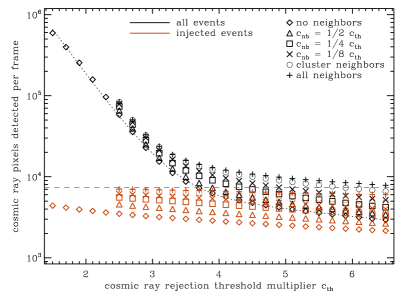
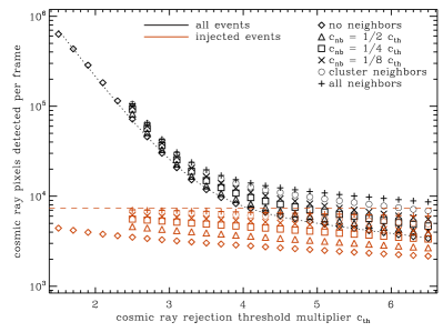
Figure 11: Number of pixels with detected outliers per frame as a function of detection thresholds $c_{th}$ and $c_{nb}$ for NRS1 (left) and NRS2 (right). The black symbols denote all detections, the red symbols are for detected events that were injected. The dashed red line shows the total number of injected events. The dotted black line denotes a fit to the data with no neighbor detection according to equation A1.

As expected, lower values of $c_{th}$ and $c_{nb}$ yield higher detection rates. In general, the total number of detected events seems to follow a two component exponential function with a knee at $c_{th}\sim 4$, rapidly increasing with low values of $c_{th}$. For the case with no neighbors (equivalent to $c_{nb}\geq c_{th}$) the number of pixels per frame with detections is well fitted by the following function:

$$n_{detections}=\alpha_{1}\times 10^{\beta_{1}c_{th}}+\alpha_{2}\times 10^{\beta_{2}c_{th}},$$ (A1)

with the parameters presented in table 5 below.

Detector	$\alpha_{1}$	$\beta_{1}$	$\alpha_{2}$	$\beta_{2}$
NRS1	$3.17\times 10^{7}$	$-1.124$	$1.06\times 10^{4}$	$-0.086$
NRS2	$2.64\times 10^{7}$	$-1.055$	$1.55\times 10^{4}$	$-0.101$

Table 5: Fit parameters for both detectors for the number of detected pixels with CRs in the case of no neighbor detection.

Detection numbers for other values of $c_{nb}$ can also be fitted by the function in equation A1, but are not shown here.

Appendix B Visual Appearance

In Figure 12 we show a region of the count rate maps of an NRS1 dark exposure in traditional readout mode with injected cosmic ray events with different cosmic ray rejection methods and thresholds:

1. no cosmic ray rejection

2. cosmic ray rejection with $c_{th}=3.5$, but no neighbors flagged

3. cosmic ray rejection with $c_{th}=3.9$ and all cluster neighbors flagged ($c_{nb}=0$)

4. cosmic ray rejection with $c_{th}=4.9$ and all neighbors flagged ($c_{nb}=0$), including neighbors of single pixels with a severe ($\geq$ 200 DN) jump in their parent

The value of $c_{th}$ was chosen to yield the best total noise for the given detection method, as presented in table 2.

Figure 12: Count rate image of a 100$\times$100 pixel region with injected CRs on NRS1 dark exposure (traditional readout). Scale is black to white from -0.1 to 0.1 DN/s. Note that the great majority of residual bright pixels in the bottom right panel are not due to undetected CRs but to the higher shot noise of hot-pixels; as can be seen in the image, they are matched by a similar number of black pixels, which are also hot-pixels (our images are dark-subtracted)

Without cosmic ray rejection, events are clearly visible and manifest as elevated count rates in usually five or more pixels. The cross-like shape of some events is due to the IPC. The centers of some cosmic ray events seem to have low count rates consistent with pixels not hit. This is due to saturation by the simulated event, so that the pixel is then flagged as saturated from that group on and the affected data is not used to determine the slope. Therefore, such events are filtered out even without jump detection.

Cosmic ray rejection without neighbor detection removes a significant fraction of cosmic rays, but tends to leave ring like structures around stronger events.

Cosmic ray rejection with flagging all cluster neighbors gives an even better visual appearance in terms of rejected cosmic rays. The leftovers are mostly the four outer pixels of five-pixel (cross-like) events. This is because, for those events, only a single pixel is identified as a CR in the first pass. Therefore, it does not qualify as belonging to a cluster and thus no neighbors are flagged (see also Figure 10).

Flagging neighbors to a single pixel, with an event (jump) of at least 200 DN, as well as cluster neighbors, gives the best visual appearance (and total noise, as shown in section 4 above).

References

- Anderson & Gordon (2011) Anderson, R. E., & Gordon, K. D. 2011, Publications of the Astronomical Society of the Pacific, 123, 1237
- Bacon et al. (2004) Bacon, C. M., McMurtry, C. W., Pipher, J. L., et al. 2004, in Society of Photo-Optical Instrumentation Engineers (SPIE) Conference Series, Vol. 5563, Infrared Systems and Photoelectronic Technology, ed. E. L. Dereniak, R. E. Sampson, & C. B. Johnson, 35–45
- Bagnasco et al. (2007) Bagnasco, G., Kolm, M., Ferruit, P., et al. 2007, in Society of Photo-Optical Instrumentation Engineers (SPIE) Conference Series, Vol. 6692, Cryogenic Optical Systems and Instruments XII, 66920M
- Beletic et al. (2008) Beletic, J. W., Blank, R., Gulbransen, D., et al. 2008, in Society of Photo-Optical Instrumentation Engineers (SPIE) Conference Series, Vol. 7021, High Energy, Optical, and Infrared Detectors for Astronomy III, 70210H
- Birkmann et al. (2016) Birkmann, S. M., Ferruit, P., Rawle, T., et al. 2016, in Society of Photo-Optical Instrumentation Engineers (SPIE) Conference Series, Vol. 9904, Space Telescopes and Instrumentation 2016: Optical, Infrared, and Millimeter Wave, 99040B
- Birkmann et al. (2018) Birkmann, S. M., Rawle, T., Ferruit, P., et al. 2018, in Space Telescopes and Instrumentation 2018: Optical, Infrared, and Millimeter Wave, Society of Photo-Optical Instrumentation Engineers (SPIE) Conference Series, 99040B
- Catalano et al. (2014) Catalano, A., Ade, P., Atik, Y., et al. 2014, Journal of Low Temperature Physics, 176, 773
- Crowley et al. (2016) Crowley, C., Kohley, R., Hambly, N. C., et al. 2016, Astronomy & Astrophysics, 595, A6
- Fadeyev et al. (2006) Fadeyev, V., Aldering, G., & Perlmutter, S. 2006, Publications of the Astronomical Society of the Pacific, 118, 907
- Fixsen et al. (2000) Fixsen, D. J., Offenberg, J. D., Hanisch, R. J., et al. 2000, Publications of the Astronomical Society of the Pacific, 112, 1350
- Gardner et al. (2009) Gardner, J. P., Mather, J. C., Clampin, M., et al. 2009, in Astrophysics in the Next Decade, ed. H. A. Thronson, M. Stiavelli, & A. Tielens, 978
- Moore et al. (2004) Moore, A. C., Ninkov, Z., & Forrest, W. J. 2004, in Society of Photo-Optical Instrumentation Engineers (SPIE) Conference Series, Vol. 5167, Focal Plane Arrays for Space Telescopes, ed. T. J. Grycewicz & C. R. McCreight, 204–215
- Offenberg et al. (1999) Offenberg, J. D., Sengupta, R., Fixsen, D. J., et al. 1999, in ASPC, Vol. 172, Astronomical Data Analysis Software and Systems VIII, ed. D. M. Mehringer, R. L. Plante, & D. A. Roberts, 141
- Rauscher et al. (2017) Rauscher, B. J., Arendt, R. G., Fixsen, D. J., et al. 2017, Publications of the Astronomical Society of the Pacific, 129, 105003
- Rauscher et al. (2014) Rauscher, B. J., Boehm, N., Cagiano, S., et al. 2014, Publications of the Astronomical Society of the Pacific, 126, 739
- Rauscher et al. (2004) Rauscher, B. J., Figer, D. F., Regan, M. W., et al. 2004, in Society of Photo-Optical Instrumentation Engineers (SPIE) Conference Series, Vol. 5487, Optical, Infrared, and Millimeter Space Telescopes, ed. J. C. Mather, 710–726
- Rauscher et al. (2007) Rauscher, B. J., Fox, O., Ferruit, P., et al. 2007, Publications of the Astronomical Society of the Pacific, 119, 768
- Rauscher et al. (2010) —. 2010, Publications of the Astronomical Society of the Pacific, 122, 1254 (Erratum)
- Regan & Bergeron (2018) Regan, M. W., & Bergeron, L. E. 2018, in Society of Photo-Optical Instrumentation Engineers (SPIE) Conference Series, Vol. 10709, 107091B
- Robberto (2010) Robberto, M. 2010, A library of simulated cosmic ray events impacting JWST HgCdTe detectors, Tech. rep., Space Telescope Science Institute
- Robberto (2014) Robberto, M. 2014, in Society of Photo-Optical Instrumentation Engineers (SPIE) Conference Series, Vol. 9143, Space Telescopes and Instrumentation 2014: Optical, Infrared, and Millimeter Wave, 91433Z
- Tylka et al. (1997) Tylka, A. J., Adams, J. J. H., Boberg, P. R., et al. 1997, IEEE Trans. Nucl. Sci., 44, 2150
- Ziegler et al. (2010) Ziegler, J. F., Ziegler, M. D., & Biersack, J. P. 2010, Nuclear Instruments and Methods in Physics Research B, 268, 1818