Uncertainty quantification and falsification of Chiral Nuclear Potentials

Abstract

Are chiral theories at present describing experimental NN scattering data satisfactorily ?. Will the chiral approach offer a framework where fitting and selecting the existing np and pp data can be done without theoretical bias ?. While predictive power in theoretical nuclear physics has been a major concern in the study of nuclear structure and reactions, the Effective Field Theory (EFT) based on chiral expansions has emerged after Weinberg as a model independent hierarchy for many body forces and much progress has been achieved over the last decades. We review some of the issues involved which point to being close to the solution, but also that work remains still to be done to validate the theory. We analyze several examples including zero energy NN scattering and perturbative counter-term-free peripheral scattering where one would expect these methods to work best and unveil relevant systematic discrepancies when a fair comparison to the Granada-2013 NN-database and partial wave analysis (PWA) based on coarse graining the interaction is undertaken.

1 Introduction

An old problem in Nuclear Physics concerns the predictive power of the theory, which is persistently much poorer than experiment. For the compiled nuclear masses one has typically $\Delta M(Z,N)^{\rm exp}<1{\rm KeV}$ Audi:2014eak . On the other hand the semi-empirical mass formula, despite being an ancient and simple model with the liquid drop model picture produces a much larger error of $\Delta M(Z,N)^{\rm th}$. Sophisticated improvements based on mean field calculations have achieved a benchmark $\Delta M(Z,N)^{\rm th}\sim 0.5{\rm MeV}$ with a large number of parameters Goriely:2016gso . After all the huge progress made in recent years in the solution of the nuclear few- and many-body problem alongside with the increasing computational power, a pending and open question remains: can this predictive power be improved by truly acknowledging all sources of uncertainties in a model independent fashion or at least incorporating some true features of Quantum Chromodynamics (QCD)?.

Of course, the best possible answer is to solve QCD directly in terms of its elementary degrees of freedom , quarks and gluons. Although much progress has been made in lattice QCD calculations with respect to the nuclear problem (see e.g. Refs. Aoki:2011ep ; Aoki:2013tba ; Aoki:2012xa for nuclear potential studies), we are still not as accurate when compared to more phenomenological approaches. One abusively refers usually to ab initio calculations to determine atomic nuclei properties in terms of their constituent nucleons. Nonetheless, there are QCD features such as chiral symmetry which may be implemented in nuclear calculations. The above question on the predictive power in Nuclear Physics still holds even if the specific constraints on chiral symmetry are explicitly taken into account.

Chiral perturbation theory for the lightest $u$ and $d$ quarks is based on the smallness of the pion mass as compared to the rest of hadronic states such as the $\rho$-meson. Indeed, the existence of a mass gap suggests that it should be possible to design an effective Hilbert space where the dynamical degrees of freedom are just pions. In addition, the fact that pions are the would-be Goldstone bosons of the spontaneously broken chiral symmetry of QCD implies that they couple derivatively, and hence they interact weakly at low momenta Weinberg:1968de . This viewpoint together with the general EFT idea Weinberg:1978kz can and has been efficiently incorporated in the simplest $\pi\pi$ system and many successes have followed Gasser:1983yg . But similarly to nuclear physics, hadronic interactions are usually characterized by a recurrent lack of predictive power on the theory side as compared to the experiments. The only known exception to this undesirable state of affairs corresponds to the theoretical determination of $\pi\pi$ scattering lengths where the theory provides an estimate which is about an order of magnitude more precise than the experiment Colangelo:2001df . This has been possible thanks to the EFT idea complemented with other properties. It is partly this spectacular success which may be taken as a strong motivation to incorporate and adapt these ideas elsewhere not only in Hadronic Physics but also in Theoretical Nuclear Physics.

When Nucleons enter the game things become more difficult and subtle from a theoretical perspective and the level of predictive power becomes more compromised because the chiral expansion converges slowly even after the regularization scheme in loop integrals is conveniently designed Gasser:1987rb ; Bernard:1992qa ; Becher:1999he . From a phenomenological point of view, in Nuclear Physics the main practical reason why chiral symmetry is not dominating could be found in the characteristic small binding energies of nucleons in atomic nuclei, $B/A=8{\rm MeV}$ or nuclear matter $B/A=16{\rm MeV}$ compared to typical hadronic scales (including the pion mass, $m_{\pi}=140{\rm MeV}$) and therefore the significance and impact of chiral symmetry is much more subtle and questionable.

From the nucleon ab initio and reductionist perspective the theoretical predictive power flow is expected to be from light to heavy nuclei. Thus, from a Hamiltonian with multi-nucleon forces

$$H(A)=T+V_{2N}+V_{3N}+V_{4N}+\dots\,,$$ (1)

one proceeds to solve the Schrödinger equation

$$H(A)\Psi_{n}=E_{n}(A)\Psi_{n}\,.$$ (2)

In the absence of useful QCD-ab initio determinations, phenomenological $V_{2N}$ interactions are adjusted to NN scattering data and the deuteron, ²H ($A=2$) and $V_{3N}$ to ³H and ³He ($A=3$), $V_{4N}$ to ⁴He (A=4) binding energies and so on. Within this setup, the chiral EFT approach to Nuclear Physics, originally pioneered by Weinberg in 1990 Weinberg:1990rz (see e.g. Bedaque:2002mn ; Epelbaum:2008ga ; Machleidt:2011zz ; Hammer:2019poc for reviews) to nuclear forces provides a power counting in terms of the pion weak decay constant $f_{\pi}=92$MeV, with the feature of systematically providing an appealing hierarchy

$$V_{2N}^{\chi}\gg V_{3N}^{\chi}\gg V_{4N}^{\chi}\gg\dots,.$$ (3)

where the irreducible contributions of a $V_{nN}^{\chi}$ potentials contain $(n-1)\pi$ exchanges as the longest range contributions. Because the pion mass is so small, chiral interactions are local and unambiguous at long distances via $1\pi$,$2\pi$,$3\pi,\dots$ exchanges for relative distances above a short distance cut-off $r_{c}$, $V^{n\pi}(r_{c})\sim e^{-nr_{c}m_{\pi}}$. Thus, if we take nuclear matter at saturation density $\rho=0.17{\rm fm}^{-3}$, the average internucleon distance is $d\equiv\rho^{-\frac{1}{3}}=1.8{\rm fm}$. We have $dm_{\pi}\sim 1.3$ and for $n\pi$ exchange by a rough suppression factor $\xi^{n}$ with $\xi=e^{-m_{\pi}d}\sim 0.3$. Of course, nucleons have a finite size and are therefore characterized by an elementary radius $r_{e}$ above which they interact as if they were elementary point-like particles characterized by local fields. For instance, for the Coulomb $pp$ interaction we have $V_{pp}(r)\sim e^{2}/r$ for $r\geq r_{e}\sim 1.8{\rm fm}$, whereas for smaller distance the overlap between protons screens the interaction due to their finite extension characterized by form factors. The numerical coincidence between $d\sim r_{e}$ makes a strong case on what may be deduced ignoring specific details for smaller distances, since for larger distances the nucleon dynamics via pion exchange can be computed explicitly using $\chi$PT. In Fig. 1 we provide a pictorial picture of the discussion above.

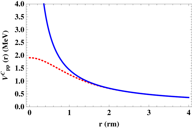
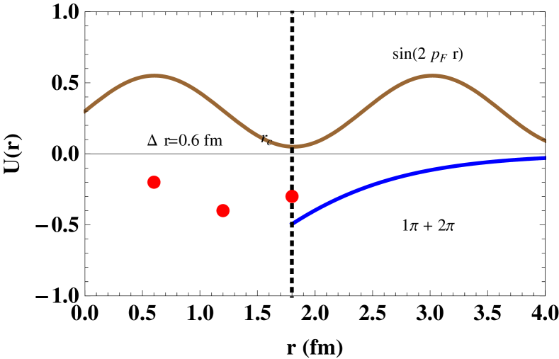
Figure 1: Top panel: Point-like (solid-blue) and extended (dashed-red) proton-proton Coulomb interaction as a function of distance. Bottom panel: Coarse grained NN potential (red dots) plus the chiral $1\pi+2\pi$ exchange potentials when $r_{c}=1.8$fm (blue line) compared with the wave function at a CM corresponding to a back-to-back NN collision on the Fermi surface in nuclear matter (brown line).

In the simplest NN case chiral potentials are constructed in perturbation theory, are universal and contain chiral constants $c_{1},c_{3},c_{4},\dots$ which can be related to $\pi N$ scattering Bedaque:2002mn ; Epelbaum:2008ga ; Machleidt:2011zz . At long distances we have

$$V^{\chi}_{NN}(r)=V^{\pi}_{NN}(r)+V^{2\pi}_{NN}(r)+V^{3\pi}_{NN}(r)+\dots\quad r\gg r_{c}\,,$$ (4)

whereas they become singular at short distances

$$V^{\chi}_{NN}(r)=\frac{a_{1}}{f_{\pi}^{2}r^{3}}+\frac{a_{2}}{f_{\pi}^{4}r^{5}}+\frac{a_{3}}{f_{\pi}^{6}r^{7}}+\dots\qquad r\ll r_{c}\,,$$ (5)

and some regularization must be introduced in any practical calculation. This feature is also in common with 3N and 4N forces. Thus the following questions arise: What is the best theoretical accuracy we can get within “reasonable” cut-offs? What is a reasonable cut-off? Can the short distance piece be organized as a power counting compatible with the chiral expansion of the long distance piece?

There has been a huge effort in the last 30 years based on the seminal work of Weinberg in theoretical nuclear physics. In essence it consists on a chiral expansion of the NN potential rather than the NN amplitude. The subject of the present work will be some reflections on the validation/falsification of NN chiral potentials when compared to existing scattering pp and np data. In the present paper we do not discuss the inner consistency of the Weinberg’s power counting, a subject which has been going on unsettled for 30 years now (see e.g. Valderrama:2019lhj for a recent discussion), but rather try to confront it with the existent NN scattering data and wonder how far are we from the claim that chiral symmetry “works” in Nuclear Physics and what is actually meant by such a statement. We will discuss here the simplest NN case, but the issues are worrisome enough to reconsider the whole approach. Motivated by this intriguing possibility we have paid dedicated attention in the last years to the issue of NN uncertainties including also chiral interactions Perez:2014kpa ; Perez:2014waa .

The topic of the present work has certainly to do with proper assessment and evaluation of uncertainties of any sort and in particular in the NN interaction and its implications. For instance, some time ago we made a first and simple estimate NavarroPerez:2012vr ; Perez:2012kt of $\Delta B^{\rm th}/A$ $\sim 0.5\,{\rm MeV}$, which has been updated in Ref. Perez:2014waa to be enlarged to $\sim 2\,{\rm MeV}$. These crude estimates are in the bulk of a more recent uncertainty analysis and order-by-order optimization of chiral nuclear interactions Carlsson:2015vda including three-body forces. These are large scale calculations where the numerical solution of the nuclear problem is very much under control, and it is found $\Delta B^{\rm th}(^{16}{\rm O})/16\sim 4{\rm MeV}$. In fact, most of the uncertainty is dominated by the cut-off variation within a “reasonable” range, but in any case it is much larger compared to the ancient 5 parameter Weiszacker semi-empirical mass formula which is based on the drop model picture, where one has $\Delta B_{\rm sem}/A\sim 0.1{\rm MeV}$. One may thus be worried that the the chiral approach to nuclear structure pioneered by Weinberg despite its theoretical appeal might actually not be very accurate despite all the new technical and conceptual sophistication which has followed thereafter.

This work is partly of review character focusing mainly on work done in Granada and adding some further aspects which have become clearer in the analysis over the last years. For many details we will refer to our previous publications along the present work. In our presentation the interaction will be characterized by a conventional quantum mechanical potential, which is not an observable itself (except for static sources) similarly to the wave function. However, contrary to what some people believe, besides being a convenient analysis tool for NN scattering with a direct application to nuclear structure calculations, its existence may be deduced from assumptions in quantum field theory which are not more restrictive than those usually made. In order to provide some scope we will review critically some of the issues concerning the link between the scattering data and the construction of the NN potential in general and the chiral potential in particular.

2 NN scattering

We will analyze pp and np scattering. We assume for simplicity of presentation the proton and neutron to have the same and common nucleon mass $M_{N}$. At fixed LAB energy $T_{\rm LAB}=2k^{2}/M_{N}$, with $k$ the CM momentum. The pion production threshold $T_{\rm LAB}=2m_{\pi}+m_{\pi}^{2}/2M_{N}\sim 290$MeV i.e. $k=370$MeV, although it has become customary to take $T_{\rm LAB}\leq 350$MeV ($k\sim 400$MeV), as the upper limit, since the inelastic cross section only becomes comparable to the elastic between single- and double-$\Delta$ production, which corresponds to the range $T_{\rm LAB}=650-1350$MeV or equivalently $k\sim 550-800$MeV, see Fig. 2. Thus, for $T_{\rm LAB}\leq 350$MeV ( $p_{\rm CM}\leq 400$MeV ) we may assume elastic scattering.

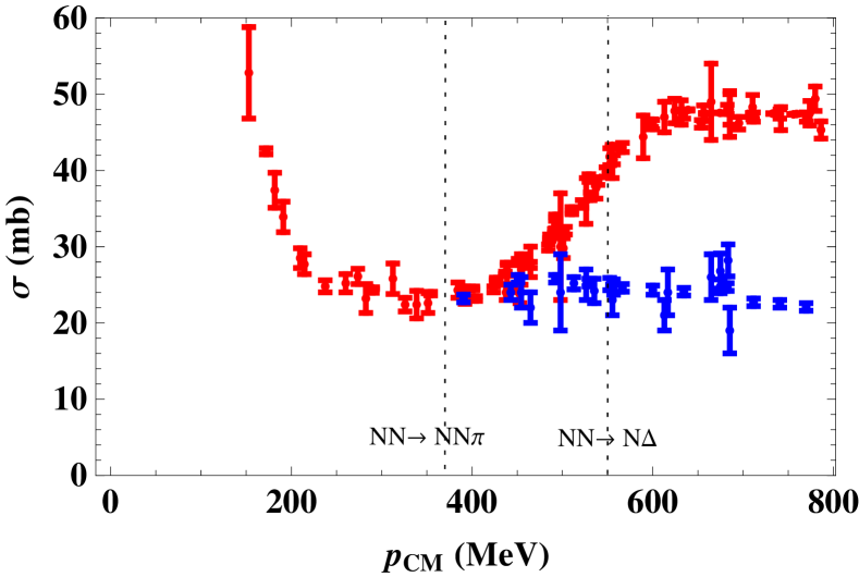
Figure 2: The pp total (red) and total elastic (blue) cross section as a function of the CM momentum. We mark the single $\pi$-production and the $\Delta$-production for reference.

2.1 The scattering amplitude

The elastic scattering process is described by the scattering matrix $S$ whose matrix elements in the CM system are defined as $S(\mathbf{\hat{k}}_{f},\mathbf{\hat{k}}_{i})\equiv\langle\mathbf{\hat{k}}_{f}|S|\mathbf{\hat{k}}_{i}\rangle$ with $\mathbf{\hat{k}}_{i}$ and $\mathbf{\hat{k}}_{f}$ the incoming and outgoing directions respectively. The unitarity of the S-matrix implies the condition

$$\delta^{(2)}(\mathbf{\hat{k}}-\mathbf{\hat{k}}^{\prime}){\bf 1}=\int d^{2}\mathbf{\hat{k}}^{\prime\prime}S(\mathbf{\hat{k}},\mathbf{\hat{k}}^{\prime\prime})S(\mathbf{\hat{k}}^{\prime\prime},\mathbf{\hat{k}}^{\prime})^{\dagger}\,,$$ (6)

where $S(\mathbf{\hat{k}}_{f},\mathbf{\hat{k}}_{i})$ is a matrix in spin-isospin space, so that we have $S(\mathbf{\hat{k}}_{i},\mathbf{\hat{k}}_{f})^{\dagger}\equiv\langle\mathbf{\hat{k}}_{f}|S^{\dagger}|\mathbf{\hat{k}}_{i}\rangle$. The NN scattering problem is analyzed in terms of the scattering amplitude $M$, defined as,

$$S(\mathbf{\hat{k}}_{f},\mathbf{\hat{k}}_{i})={\bf 1}+2kiM(\mathbf{\hat{k}}_{f},\mathbf{\hat{k}}_{i})\,.$$ (7)

If we impose P (Parity),T (Time Reversal) and Lorentz invariance symmetries, the complete on-shell NN scattering amplitude contains five independent complex quantities, which we choose for definiteness as the Wolfenstein parameters glockle1983quantum

$$M(\mathbf{\hat{k}}_{f},\mathbf{\hat{k}}_{i}) = a+m(\mathbf{\sigma}_{1}\cdot\mathbf{n})(\mathbf{\sigma}_{2}\cdot\mathbf{n})+(g-h)(\mathbf{\sigma}_{1}\cdot\mathbf{m})(\mathbf{\sigma}_{2},\mathbf{m})$$ (8)

$$+(g+h)(\mathbf{\sigma}_{1}\cdot\mathbf{l})(\mathbf{\sigma}_{2}\cdot\mathbf{l})+c(\mathbf{\sigma}_{1}+\mathbf{\sigma}_{2})\cdot\mathbf{n}\,,$$

where $a,m,g,h,c$ depend on energy and angle, $\mathbf{\sigma}_{1}$ and $\mathbf{\sigma}_{2}$ are the single nucleon Pauli matrices, $\mathbf{l}$, $\mathbf{m}$, $\mathbf{n}$ are three unitary orthogonal vectors along the directions of $\mathbf{\hat{k}}_{f}+\mathbf{\hat{k}}_{i}$, $\mathbf{\hat{k}}_{f}-\mathbf{\hat{k}}_{i}$ and $\mathbf{\hat{k}}_{f}\wedge\mathbf{\hat{k}}_{i}$ and $\mathbf{k}_{f}=k\mathbf{\hat{k}}_{f}$, $\mathbf{k}_{i}=k\mathbf{\hat{k}}_{i}$ are the final and initial relative nucleon momenta respectively. The amplitudes $a,m,g,h,c$ could in principle be determined directly from experiment as shown in Ref. Hoshizaki:1969qt ; Bystricky:1976jr ; LaFrance:1981bg (see also  kamada2011 for an exact analytical inversion). In writing this amplitude, use has been made of the on-shell elastic condition $k_{f}=k_{i}$ which implies the identity okubo1958velocity ,

$$\mathbf{\sigma_{1}}\cdot\mathbf{\sigma_{2}}=(\mathbf{\sigma}_{1}\cdot\mathbf{l})(\mathbf{\sigma}_{2}\cdot\mathbf{l})+(\mathbf{\sigma}_{1}\cdot\mathbf{m})(\mathbf{\sigma}_{2}\cdot\mathbf{m})+(\mathbf{\sigma}_{1}\cdot\mathbf{n})(\mathbf{\sigma}_{2}\cdot\mathbf{n})$$ (9)

As a consequence of unitarity we have the relation

$$M(\mathbf{\hat{k}}_{f},\mathbf{\hat{k}}_{i})-M(\mathbf{\hat{k}}_{f},\mathbf{\hat{k}}_{i})^{\dagger}=2ik\int d^{2}\hat{k}_{n}M(\mathbf{\hat{k}}_{f},\mathbf{\hat{k}}_{n})M(\mathbf{\hat{k}}_{n},\mathbf{\hat{k}}_{i})^{\dagger}\,.$$ (10)

If we go to the orthonormal basis of eigenstates $\phi_{n}(\mathbf{\hat{k}})$ with eigenvalues $M_{n}$ the spectral decomposition reads

$$M(\mathbf{\hat{k}}_{f},\mathbf{\hat{k}}_{i})=\sum_{n}M_{n}\phi_{n}(\mathbf{\hat{k}}_{f})\phi_{n}(\mathbf{\hat{k}}_{i})^{\dagger}\,,$$ (11)

so that we can write the unitarity condition as $M_{n}=K_{n}/(1-ikK_{n})$ with $K_{n}$ real, and define the self-adjoint operator

$$K(\mathbf{\hat{k}}_{f},\mathbf{\hat{k}}_{i})=\sum_{n}K_{n}\phi_{n}(\mathbf{\hat{k}}_{f})\phi_{n}(\mathbf{\hat{k}}_{i})^{\dagger}$$ (12)

and we have the integral equation

$$M(\mathbf{\hat{k}}_{f},\mathbf{\hat{k}}_{i})=K(\mathbf{\hat{k}}_{f},\mathbf{\hat{k}}_{i})+ik\int d^{2}\hat{k}_{n}K(\mathbf{\hat{k}}_{f},\mathbf{\hat{k}}_{n})M(\mathbf{\hat{k}}_{n},\mathbf{\hat{k}}_{i})\,.$$ (13)

The $K-$matrix has the same decomposition as the scattering amplitude but now the coefficients are real which means that scattering at a given energy and angle can be described by 5 independent real functions.

2.2 Analytical properties

To these properties, one has to add the existence of analytical properties in the scattering energy and angle, or equivalently in the Mandelstam variables $t=-(\mathbf{k}_{f}-\mathbf{k}_{i})^{2}$ and $s=4(k^{2}+M_{N}^{2})$ in the complex plane. This corresponds to a Mandelstam double spectral representation of the scattering amplitude Mandelstam:1959bc which actually provides a justification for using interpolation methods in phenomenological analyses. These important constraints are explicitly satisfied in field theory in perturbation theory, where interactions arise from particle exchange and at long distances pion exchanges dominate. Unfortunately, the unitarity of the S-matrix is not preserved exactly in perturbation theory and several unitarization methods have been proposed. While all these elements provide a framework to describe the scattering problem it does not give a direct hint about the NN interactions from which nuclear binding energies might be determined. It should be noted that for quantum mechanical potentials being a superposition of Yukawa potentials the double spectral representation holds for elastic scattering Blankenbecler:1960zz and also in the presence of inelasticities described by a complex and energy dependent optical potential cornwall1962mandelstam ; omnes1965optical . This issue has been exemplified recently in the case of $\pi\pi$-scattering RuizdeElvira:2018hsv .

2.3 The partial wave expansion

The NN scattering amplitude conserves the total angular momentum $\vec{J}=\vec{L}+\vec{S}$, the spin $(\vec{S})^{2}$, and hence a complete set of commuting observables is given by $\{J^{2},J_{z},S^{2}\}$ so that a convenient basis is given by the vector spherical harmonics ${\cal Y}_{JLSM}(\hat{k})$, so that

$$S\,{\cal Y}_{JLSM}(\hat{k})=\sum_{L^{\prime}}S^{J,S}_{L,L^{\prime}}{\cal Y}_{JL^{\prime}SM}(\hat{k}).$$ (14)

The analysis of NN scattering has been traditionally carried out by a decomposition of the scattering amplitude in partial waves. For this amplitude the partial wave expansion in this case reads

$$M^{s}_{m_{s}^{\prime},m_{s}}(\theta) =\frac{1}{2ik}\sum_{J,l^{\prime},l}\sqrt{4\pi(2l+1)}Y^{l^{\prime}}_{m_{s}^{\prime}-m_{s}}(\theta,0)$$

$$\times C^{l^{\prime},S,J}_{m_{s}-m_{s}^{\prime},m_{s}^{\prime},m_{s}}i^{l-l^{\prime}}(S^{J,S}_{l,l^{\prime}}-\delta_{l^{\prime},l})C^{l,S,J}_{0,m_{s},m_{s}},$$ (15)

where $S$ is the unitary coupled channel S-matrix, and the $C^{\prime}s$ are Clebsch-Gordan coefficients. Denoting the phase shifts as $\delta^{J,s}_{l,l^{\prime}}$, for the singlet ($s=0$, $l=l^{\prime}=J$) and triplet uncoupled ($s=1$, $l=l^{\prime}=J$) channels the $S$ matrix is simply $e^{2i\delta^{J,s}_{l,l}}$, in the triplet coupled channel ($s=1$, $l=J\pm 1$, $l^{\prime}=J\pm 1$) it reads

$$S^{J}=\left(\begin{array}[]{c c}e^{2i\delta^{J,1}_{J-1}}\cos{2\epsilon_{J}}&ie^{i(\delta^{J,1}_{J-1}+\delta^{J,1}_{J+1})}\sin{2\epsilon_{J}}\\ ie^{i(\delta^{J,1}_{J-1}+\delta^{J,1}_{J+1})}\sin{2\epsilon_{J}}&e^{2i\delta^{J,1}_{J+1}}\cos{2\epsilon_{J}}\end{array}\right),$$ (16)

with $\epsilon_{J}$ the mixing angle.

Because of unitarity one has that ${\bf S}^{JS}=({\bf M}^{JS}-i{\bf 1})({\bf M}^{JS}+i{\bf 1})^{-1}$ with $({\bf M}^{JS})^{\dagger}={\bf M}^{JS}$ a hermitian coupled channel matrix (also known as the K-matrix). The main advantage is that for finite range interactions of range $a$ one expects the partial wave sum to be truncated at about $L_{\rm max}+1/2\sim ka$.

As mentioned, the NN scattering amplitude has 5 independent complex components for any given energy, which must and can be determined from a complete set of measurements involving differential cross sections and polarization observables. While this is most often done in terms of phase-shifts, it is worth reminding that phase shifts obtained in PWA are not observables by themselves. This is so unless a complete set of 10 fixed energy and angle dependent measurements have been carried out. This is a rare case among the bunch of existing 8000 np+pp scattering data below $350\,{\rm MeV}$ LAB energy and which corresponds to a maximal CM momentum of $p_{\rm CM}^{\rm max}=2{\rm fm}^{-1}$. In order to intertwine all available, often incomplete and partially self-contradictory, information some energy interpolation is needed. The situation is illustrated by the abundance plots in Fig. 3 (see top and bottom left panels) where every point represents a measured observable (cross section, polarization, etc.) of a total of about 8000 pp+np data. Thus, the fact that the energy dependence of the amplitude is not completely arbitrary will be most helpful.

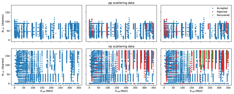
Figure 3: Abundance plots for pp (top panels) and np (bottom panels) scattering data. Full data base (left panel). Standard $3\sigma$ criterion (middle panels). Self-consistent $3\sigma$ criterion (right panels). We show accepted data (blue), rejected data (red) and recovered data (green).

At the level of partial waves the multi-pion exchange diagrams generate left hand cuts in the complex s-plane, which come in addition to the NN elastic right cut and the $\pi NN$, $2\pi NN$ etc., pion production cuts,as can be seen in Fig. 4. At low energies for $|p|\leq m_{\pi}/2$ the scattering amplitude is analytic and we have the Taylor expansion PavonValderrama:2005ku

$$p^{l+l^{\prime}+1}M_{l,l^{\prime}}^{JS}(p)=-(\alpha^{-1})^{JS}_{l,l^{\prime}}+\frac{1}{2}(r_{0})^{JS}_{l,l^{\prime}}p^{2}+\sum_{n=2}^{\infty}(v_{2n})^{JS}_{l,l^{\prime}}p^{2n}$$ (17)

An implementation of these analytical properties can be done in terms of dispersion relations for short range interactions and thus leaving out the important case of long range interactions such as Coulomb and magnetic moments interactions. In Fig. 4 we depict a characteristic contour which in fairness would be needed for encompassing the available data with $T_{\rm LAB}\leq 350$MeV along the unitarity cut but also up to about $5\pi$-exchange to faithfully describe the left hand cut within the same contour. At present only $3\pi$ exchanges have been considered starting by Ref. Pupin:1999ba . A particularly attractive scheme to represent the analytical properties is given by the so-called N/D method, where the partial wave amplitude is represented as a ratio between two functions $N(s)$ which has only left-cut (particle exchange) discontinuities and $D(s)$ which has only right-cut (unitarity) discontinuities. While this method has been around for over 50 years, in the NN case the resulting set of integral equations required from multi-pion exchange are highly singular at short distances and only a suitable subtraction hierarchy allows to handle the singularities (see e.g. Oller:2018zts and references therein). These conclusions have a parallel developement in terms of a quantum mechanical potential for the renormalization in coordinate space PavonValderrama:2005wv ; PavonValderrama:2005uj and the $N/D$ representation RuizdeElvira:2018hsv .

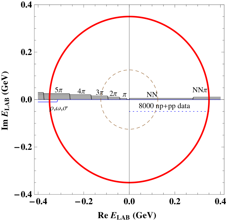
Figure 4: The LAB energy complex plane, showing the partial waves left cut structure due to multiple pion (and $\sigma,\rho\omega$) exchange along with the right cut structure due to pion production. $T_{\rm LAB}^{\rm left}=(\dots,-375.3,-260.6,-166.8,-93.8,-41.7,-10.4){\rm MeV}$. The outer/inner circles correspond to LAB energies of $350/125$MeV respectively.

3 The NN potential

3.1 The use of a potential

One of the good reasons to discuss the NN scattering problem is to design suitable NN interactions which can be used in few and many body calculations and in particular address the problem of binding in atomic nuclei. In the most popular Hamiltonian approach the interaction is characterized by a potential. Moreover, provided the potential fulfills a spectral representation as a superposition of Yukawa One Pion Exchange (OPE) form, the scattering amplitude can be shown to posses analytical properties in both the CM energy and the scattering angle (or equivalently Mandelstam $s,t$ variables), which also guarantees the smoothness in a given energy interpolation which proves useful in fitting data.

For LAB energies below $350$MeV relativity plays a small but significant role (relativistic Coulomb corrections will be needed). The proper incorporation of relativity requires also to take into account retardation effects. The standard Bethe-Salpeter equation Salpeter:1951sz is an exact four-dimensional integral equation which besides facing technical difficulties poses theoretical issues in practice since any finite truncation of irreducible diagrams generates spurious effects and inconsistencies in the amplitude or generate fake results in the heavy-light limiting case. One may consider instead three dimensional reductions of the Blankenblecker-Sugar Blankenbecler:1965gx , Gross Gross:1969rv or Kadyshevsky form Kadyshevsky:1967rs , among the many possible schemes, fulfilling special properties. This relativistic ambiguity would come in addition to several ones discussed below.

Assuming from now on the non-relativistic case, NN scattering is formulated in terms of the Lippmann-Schwinger (LS) equation which at the operator level reads

$$T(E)=V+VG_{0}T(E)\,,$$ (18)

where $H_{0}$ is the free Hamiltonian and $V$ is the potential and $E=k^{2}/2\mu$ is the CM energy and $G_{0}=(E-H_{0})^{-1}$. Inserting a complete set of states we have

$$\langle\mathbf{p}^{\prime}|T(E)|\mathbf{p}\rangle =\langle\mathbf{p}^{\prime}|V|\mathbf{p}\rangle$$ (19)

$$+\int\frac{d^{3}p^{\prime\prime}}{(2\pi)^{3}}\langle\mathbf{p}^{\prime}|V|\mathbf{p}^{\prime\prime}\rangle\frac{1}{E-E_{p^{\prime\prime}}}\langle\mathbf{p}^{\prime\prime}|T(E)|\mathbf{p}\rangle\,.$$

Then, taking the on-shell conditions, we get

$$M(\hat{\mathbf{p}}^{\prime},\hat{\mathbf{p}})=-\frac{\mu}{2\pi}\langle\mathbf{p}^{\prime}|T(E)|\mathbf{p}\rangle|_{|p^{\prime}|=|p|=k}\,.$$ (20)

Note that although Eq. (13) and Eq.(19) look very similar they are in fact rather different since the second equation contains in addition an integral over the energy, and thus the relation between $K$ and $V$ is an integral equation. The LS framework generates therefore an ambiguity in the potential, i.e. there are infinitely many potentials which generate the same on-shell scattering amplitude. While we may use this freedom to impose certain convenient conditions, one must not abuse this possibility since it may introduce a bias in the analysis of the data. Being ourselves theoreticians, we take the practical point of view that the least biased choice of the interaction corresponds to the one allowing to congregate as many data as possible, rather than pondering on the correctness of the many experiments.

From a purely mathematical perspective, the inverse scattering problem concerns the determination of such a potential directly from the scattering data chadan2012inverse . As such, the solution of this problem is ambiguous and additional conditions need to be imposed to fix this ambiguity. In practice, implementing this approach requires a parameterization of the scattering amplitude interpolating between different measured points, which becomes rather involved and may require a large number of interpolating parameters if high precision is required.

As we will review below, the scheme which is usually employed is to make instead a least squares determination of a proposed form of the potential in terms of the measured scattering observables which may be validated or falsified in a statistical sense. Such an approach has allowed to describe about 7000 np+pp scattering measurements below $T_{\rm LAB}=350{\rm MeV}$ with a number of about 30-50 parameters which a high degree of confidence. Of course, in the case that a given NN potential is validated, error analysis applies and experimental errors can be propagated to any predicted quantity.

3.2 NN potential components

Assuming isospin invariance, the most general form of the NN interaction can be written as okubo1958velocity

$$V({\mathbf{p}}~{}^{\prime},\mathbf{p}) =\>\,V_{C}\>\,+\vec{\tau}_{1}\cdot\vec{\tau}_{2}\,W_{C}$$

$$+\left[\,V_{S}\>\,+\vec{\tau}_{1}\cdot\vec{\tau}_{2}\,W_{S}\,\>\,\right]\,\vec{\sigma}_{1}\cdot\vec{\sigma}_{2}$$

$$+\left[\,V_{LS}+\vec{\tau}_{1}\cdot\vec{\tau}_{2}\,W_{LS}\right]\,\left(-i\vec{S}\cdot(\mathbf{q}\times\mathbf{P})\,\right)$$

$$+\left[\,V_{T}\>\,+\vec{\tau}_{1}\cdot\vec{\tau}_{2}\,W_{T}\,\>\,\right]\,\vec{\sigma}_{1}\cdot\mathbf{q}\,\,\vec{\sigma}_{2}\cdot\mathbf{q}$$

$$+\left[\,V_{Q}+\vec{\tau}_{1}\cdot\vec{\tau}_{2}\,W_{Q}\,\right]\,\vec{\sigma}_{1}\cdot(\mathbf{q}\times\mathbf{P}\,)\,\,\vec{\sigma}_{2}\cdot(\mathbf{q}\times\mathbf{P}\,)$$

$$+\left[\,V_{P}+\vec{\tau}_{1}\cdot\vec{\tau}_{2}\,W_{P}\,\right]\,\vec{\sigma}_{1}\cdot\mathbf{P}\,\,\vec{\sigma}_{2}\cdot\vec{P}\,\,,$$ (21)

where ${\mathbf{p}}\,^{\prime}$ and $\mathbf{p}$ denote the final and initial nucleon momenta in the CMS, respectively. Moreover, $\mathbf{q}={\mathbf{p}}\,^{\prime}-\mathbf{p}$ is the momentum transfer, $\mathbf{P}=({\mathbf{p}}\,^{\prime}+\mathbf{p})/2$ the average momentum, and $\vec{S}=(\vec{\sigma}_{1}+\vec{\sigma}_{2})/2$ the total spin, with $\vec{\sigma}_{1,2}$ and $\vec{\tau}_{1,2}$ the spin and isospin operators, of nucleon 1 and 2, respectively.

For the on-shell situation, $V_{i}$ and $W_{i}$ (where $i$ is equal to $C$, $S$, $LS$, $T$, $Q$ or $P$) can be expressed as functions of $q=|\mathbf{q}\,|$ and $p=|{\mathbf{p}}\,^{\prime}|=|\mathbf{p}\,|$, only. As pointed out in Ref. okubo1958velocity the terms corresponding to $V_{P}$ and $W_{P}$ can be re-written in terms of other operators provided particles are on-shell, i.e. $\mathbf{P}\cdot\mathbf{q}=p^{\prime 2}-p^{2}=0$. However, this is in general not the case. For instance the exchange of an $A_{1}$ meson does produce such a contribution to order $1/M_{N}^{2}$.

The calculation of the potential stemming from field theory always proceeds by matching the perturbative solution of the quantum mechanical problem to a perturbative calculation of Feynman diagrams in quantum field theory Logunov:1963yc . For instance, the leading contribution in our sign-convention is such that the one-pion exchange contribution in is of the form $W_{T}^{(1\pi)}=-(g_{\pi N}/2M_{N})^{2}(m_{\pi}^{2}+q^{2})^{-1}$, with the physical values of the coupling constant $g_{\pi N}$ and the nucleon and pion masses $M_{N}$ and $m_{\pi}$. In general, for a quantum field theory (QFT) calculation organized in the perturbative expansion

$$T|_{\rm QFT}=T_{1}+T_{2}+\cdots$$ (22)

we assume a similar expansion of the potential

$$V=V_{1}+V_{2}+\cdots$$ (23)

such as the perturbative solution of the LS equation, Eq. (18) is identified order by order

$$V_{1} =T_{1}$$

$$V_{2} =T_{2}-V_{1}G_{0}V_{1}$$

$$V_{3} =T_{3}+V_{1}G_{0}V_{1}G_{0}V_{1}-V_{2}G_{0}V_{1}-V_{1}G_{0}V_{2}$$

$$\dots$$ (24)

This procedure introduces ambiguities, since strictly speaking only the resulting on-shell scattering amplitude is uniquely defined. Therefore, there is no unique way of determining the potential, even in perturbation theory, a perturbative reminiscent feature from the inverse scattering problem. The remaining freedom can be used advantageously to choose a particular form of the potential by means of suitable unitary transformations Amghar:2002pf . The advantage is that the potential may be tailored to be used within a given computational scheme solving the nuclear problem for finite nuclei. In a broader context one should, however, keep in mind that this has also some implication on the 3N problem, since the very definition of a three-body force is based on the definition of the two-body interaction.

As it is well known, unitarity is not preserved exactly in perturbation theory, only order by order. Therefore, the identification of scattering quantities, say the phase-shifts, is not unique. From this point of view one of the motivations to proceed via the potential, is that unitarity is restored at any order of the calculation, since the total amplitude corresponds to a particular re-summation method. Again, the unitarization method is not unique, and different re-summation schemes yield different results (see e.g. Ref. Nieves:1999bx for a discussion in the $\pi\pi$ case). A good example is the choice of the 3D reduction of a relativistic scattering equation for which several possibilities exist.

Moreover, perturbation theory is based on the smallness of a coupling constant; the amplitude is parametrically small when the coupling constant tends to zero. The real convergence for a finite coupling constant is another issue, and one may wonder under what physical conditions does a perturbative calculation provide sensible results. Naively, we should expect small angles scattering, or equivalently $q\to 0$, to be the relevant situation. In practice the finite pion mass, requires the unphysical limit $q\to im_{\pi}$ for the OPE contribution to dominate over the other contributions, but there is no measurable kinematic region where for instance the coupling constant can be determined from the OPE potential alone; either some extrapolation from the data into the unphysical region is needed or a short range contribution must be included to fit experimental data. At present the most accurate determination to data uses the second method Perez:2016aol ; Arriola:2016hfi . The small angle limit corresponds at the partial waves level to large angular momentum states and in the classical limit to a large impact parameter. These states are not measured directly but rather deduced from a PWA. We will comment on this issue below in more detail when discussing peripheral waves.

3.3 Semi-local Potentials

The scalar functions appearing in the potential, Eq. (21), depend on both initial and final momentum $\vec{p}$ and $\mathbf{p}^{\prime}$ respectively. Because of rotational invariance we may thus form three independent invariants, such as $p,p^{\prime}$ and also $\mathbf{q}\cdot\mathbf{P}$ (which vanishes on-shell). Passing to coordinate space in the conjugate variable of $q$ we have

$$V(\mathbf{r},\mathbf{P})=\int\frac{d^{3}q}{(2\pi)^{3}}e^{i\mathbf{q}\cdot\mathbf{r}}\langle\mathbf{P}+\frac{1}{2}\mathbf{q}|V|\mathbf{P}-\frac{1}{2}\mathbf{q}\rangle\,,$$ (25)

where we take $\langle\mathbf{P}+\frac{1}{2}\mathbf{q}|V|\mathbf{P}-\frac{1}{2}\mathbf{q}\rangle\equiv V(\mathbf{p}^{\prime},\mathbf{p})$. The case where these functions depend only on the momentum transfer $\mathbf{q}=\mathbf{p}^{\prime}-\mathbf{p}$ corresponds in coordinate space to a local potential, $V(\mathbf{r},\mathbf{P})=V(\mathbf{r})$. This has the appealing property that the quantum mechanical problem becomes a differential equation which can be solved very efficiently after imposing regularity conditions of the wave function at the origin. Moreover, important long-range effects such as the Coulomb interaction or the magnetic moments interaction are local and the incorporation in coordinate space is straightforward and much less painful than in momentum space. However, imposing this particular form is a restriction which might introduce a bias in the statistical analysis of the scattering data. In the general case, the presence of polynomials in $P$ implies that the potential is also a differential operator, as can be checked by taking the corresponding Fourier transformation.

There is a limiting case, however, where we expect the potential to be truly local and actually an observable. Indeed, attaching a field theoretical interpretation to the interaction, locality must be satisfied by heavy and point-like elementary nucleons which act as static sources. In this case, the static energy between them corresponds to the potential

$$E_{NN}(r)=V_{NN}(r)+2M_{N}+{\cal O}(M_{N}^{-1})\,,$$ (26)

where we assume $M_{N}\gg m_{\pi},E$. Thus, we expect finite nucleon mass effects to be responsible for non-localities, which means that we will have the combination $P/M_{N}$. Thus, it makes sense to assume a polynomial in $P/M_{N}$, which upon transformation into Fourier space will make the potential a differential operator. This form has been frequently used in the past up to ${\cal O}(P^{2})$ because it still corresponds to a second order differential equation, in the generalized Sturm-Liouville form with the standard regularity conditions at the origin (see e.g. Ref. Piarulli:2016vel ). However, to order ${\cal O}(P^{4})$ or higher, one should impose regularity conditions and the wave function and higher derivatives; this is perhaps the reason why to our knowledge it has never been implemented. The momentum space approach, however, does not require explicitly these boundary conditions at the origin, and this is the preferred form in case of strong non-locality.

As already mentioned, it is possible, by means of suitable unitary transformations Amghar:2002pf to transfer the operators $P$ into angular momentum operators, at least to ${\cal O}(P^{2})$, which act matrix-multiplicatively on the partial wave basis and hence no derivatives of the wave function need to be evaluated. In practice, phenomenological and chiral potentials may be taken to be weakly nonlocal or semi-local. The computational advantages for a local interaction have been exploited in the Argonne potentials saga which were specifically designed to favor MonteCarlo calculations.

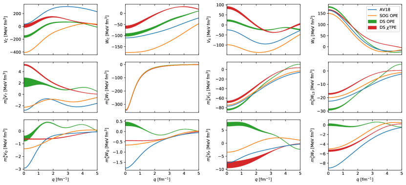
Figure 5: Momentum space components of potentials as a function of the momentum transfer for several potentials: AV18 Wiringa:1994wb and the Granada DS-OPE Perez:2013mwa ; Perez:2013jpa , DS-$\chi$TPE Perez:2013oba ; Perez:2013cza and Gauss-OPE Perez:2014yla .

In the Argonne basis, the potential containing at most two powers of momentum can be written as

$$V=\sum_{n=1}^{21}O_{n}V_{n}(r)\,,$$ (27)

where the operators $O_{n}$ contain the linear momentum operator only through the angular momentum operator $\vec{L}=\mathbf{r}\wedge\mathbf{p}$ and are matrix-multiplicative when acting on the partial wave basis, i.e.

$$O_{n}{\cal Y}_{JLSM}(\hat{r})=\sum_{L^{\prime}}(O_{n})_{L,L^{\prime}}^{JS}{\cal Y}_{JL^{\prime}SM}(\hat{r}).$$ (28)

This can be generalized to higher orders in $p$ or equivalently in $L$. Here, the first fourteen operators are the same charge-independent ones used in the Argonne $v_{14}$ potential and are given by

$$O^{n=1,14} =1,{\tau}_{1}\!\cdot\!{\tau}_{2},\,{\sigma}_{1}\!\cdot\!{\sigma}_{2},({\sigma}_{1}\!\cdot\!{\sigma}_{2})({\tau}_{1}\!\cdot\!{\tau}_{2}),\,S_{12},S_{12}({\tau}_{1}\!\cdot\!{\tau}_{2}),\,$$

$${\bf L}\!\cdot\!{\bf S},{\bf L}\!\cdot\!{\bf S}({\tau}_{1}\!\cdot\!{\tau}_{2}),L^{2},L^{2}({\tau}_{1}\!\cdot\!{\tau}_{2}),\,L^{2}({\sigma}_{1}\!\cdot\!{\sigma}_{2}),$$

$$L^{2}({\sigma}_{1}\!\cdot\!{\sigma}_{2})({\tau}_{1}\!\cdot\!{\tau}_{2}),\,({\bf L}\!\cdot\!{\bf S})^{2},({\bf L}\!\cdot\!{\bf S})^{2}({\tau}_{1}\!\cdot\!{\tau}_{2})\ .$$ (29)

These fourteen components are denoted by the abbreviations $c$, $\tau$, $\sigma$, $\sigma\tau$, $t$, $t\tau$, $ls$, $ls\tau$, $l2$, $l2\tau$, $l2\sigma$, $l2\sigma\tau$, $ls2$, and $ls2\tau$. The remaining terms are

$$O^{n=15,21} =T_{12},\,({\sigma}_{1}\!\cdot\!{\sigma}_{2}),T_{12}\,S_{12}T_{12},\,(\tau_{z1}+\tau_{z2})\ ,$$

$$({\sigma}_{1}\!\cdot\!{\sigma}_{2})(\tau_{z1}+\tau_{z2})\ ,L^{2}T_{12},L^{2}({\sigma}_{1}\!\cdot\!{\sigma}_{2})T_{12}\,.$$ (30)

These terms are charge dependent and are labeled as $T$, $\sigma T$,$tT$, $\sigma\tau z$, $l2T$ and $l2\sigma T$.

3.4 Momentum space representation

The relation between the Argonne basis and the momentum space representation in Eq. (21) can be found passing to momentum space

$$\langle\mathbf{p}^{\prime}|V|\mathbf{p}\rangle\equiv\int\frac{d^{3}r}{(2\pi)^{3}}e^{-i\mathbf{p}^{\prime}\cdot\vec{r}}Ve^{i\mathbf{p}\cdot\vec{r}}=\sum_{n}\tilde{O}_{n}(q,P)\tilde{V}_{n}(q)$$ (31)

We list the basic Fourier transforms in the Appendix A and operator transforms (see e.g. Ref. Veerasamy:2011ak ). Two aspects deserve attention, off-shellness and locality. In general the 12 components depend on the scalars $q,\mathbf{P}\cdot\mathbf{q},P$ and they reduce to just 10 when the on-shell condition $\mathbf{P}\cdot\mathbf{q}=0$ is taken. The local approximation corresponds to take $\mathbf{P}=0$ which includes also the on-shell condition. In Fig. 5 we depict the 12 components for the AV18 potential Wiringa:1994wb in the local approximation. We see that while not all potentials are of the same size, all allowed components are non-vanishing. This observation will be useful when analyzing the implications of power counting and chiral symmetry.

Off-shell $k_{f}\neq k_{i}$ and $\sigma_{1}\cdot\sigma_{2}$ enters as an independent additional operator combination, since the on-shell identity, Eq. (9) does not hold. Another feature is that the off-shell independent components $V_{P}$ and $W_{P}$ are significantly non-vanishing.

3.5 The separation distance

Once the form of the (semi-local) potential is specified, the radial dependence of the components $V_{n}(r)$ must be determined. We have taken a sharp separation distance, $r_{c}$, where we distinguish between the known and calculable part of the potential, by invoking QFT with hadronic degrees of freedom, and the unknown part which should not be calculable at the hadronic level, since it involves finite size, quark overlap and exchange terms, etc. Obviously, for a model independent analysis this separation distance should not be smaller than the elementary radius, $r_{e}$, i.e., the distance above which particles may be regarded as point like (see e.g. Fig. 1). The analysis of Ref. Arriola:2016hfi based on quark cluster considerations and the nucleon and $N\Delta$ transition form factors suggest that also that $r_{e}\sim 1.8$fm. Thus, the separation reads,

$$V(r)=V_{\rm short}(r)\theta(r_{c}-r)+V_{\rm QFT}(r)\theta(r-r_{c})\,,$$ (32)

Although it has become customary to use smooth radial functions, their particular shape may mask finite size features, and thus in all our studies we insist on this sharp separation scheme. While the long range part contains and discriminates between strong and electroweak contributions, the short range part contains both contributions and we will make no effort to disentangle them explicitly.

3.6 The number of independent parameters

In order to deal with the short distance components we may in principle propose some functions with “reasonable” shapes characterized by some parameters as it is, e.g., the case of the AV18 potential Wiringa:1994wb . As we will discuss below, uncertainties in the potential are actually dominated by the arbitrariness in the representation of the potential at short distances. To overcome this difficulty we have appealed in our analyses to the use of coarse grained potentials, a scheme proposed long ago by Avilés Aviles:1973ee and rediscovered in Ref. Entem:2007jg (see e.g.Ref. NavarroPerez:2011fm ; RuizArriola:2019pwt for pedagogical discussions). This approach is inspired by a Wilsonian point of view and an optimal sampling of the potential is implemented after Nyquist theorem. We take a grid of equidistant radial “thick” points in coordinate space separated by the finite resolution given by the shortest de Broglie wavelength, $\Delta r=\hbar/p_{\rm CM}^{\rm max}\sim 0.6{\rm fm}$ up to the radius $r_{c}=3\,{\rm fm}$, above which charge dependent $1\pi$ exchange gives the entire strong contribution. This gives, for instance, for an S-wave $r_{c}/\Delta r=5$ thick points. A simple calculation including all active partial waves, $L\lesssim pr_{c}$, yields the estimate Fernandez-Soler:2017kfu ; RuizArriola:2019pwt ,

$$N_{\rm Par}\sim\frac{1}{2}(p_{\rm CM}^{\rm max}r_{c})^{2}\,g_{S}\,g_{T}\,,$$ (33)

where $g_{S}$ and $g_{T}$ are spin and isospin degeneracy factors. The counting of parameters for pp and np Perez:2013cza yields about 40 “thick” points $r_{n}$ if the fit is carried up to a maximal $T_{\rm LAB}\leq 350$MeV. This a priori estimate coincides with the bulk of parameters which have been needed to fit data satisfactorily in the past. The simplest way these thick points may be represented by delta-shells (DS) NavarroPerez:2012qf as originally proposed by Avilés Aviles:1973ee , and the potential values at these points $V_{i}(r_{n})$ are taken as the fitting parameters,

$$V_{\rm short}(r)=\sum_{n,i}\Delta r\,O_{n}\,V_{n}(r_{i})\delta(r-r_{i})\,.$$ (34)

Of course, the estimate Eq. (33), shows that in order to minimize the number of parameters for a given maximal momentum the value of $r_{c}$ should be taken as smallest as possible, but never smaller then the elementary radius, $r_{e}\sim 1.8$fm.

3.7 The long range contributions

The hadronic QFT calculable contribution is separated into two pieces, the strong (pion exchange) piece and the purely EM piece,

$$V_{\rm QFT}=V_{\pi}(r)+V_{\rm EM}(r)\,.$$ (35)

The charge dependent OPE potential in the long range part of the interaction is the same as the one used by the Nijmegen group on their 1993 PWA Stoks:1993tb and reads

$$V_{m,\rm OPE}(r)=f^{2}\left(\frac{m}{m_{\pi^{\pm}}}\right)^{2}\frac{1}{3}m\left[Y_{m}(r){\mathbf{\sigma}}_{1}\cdot\mathbf{\sigma}_{2}+T_{m}(r)S_{1,2}\right]$$ (36)

being $f$ the pion coupling constant, ${\mathbf{\sigma}}_{1}$ and ${\mathbf{\sigma}}_{2}$ the single nucleon Pauli matrices, $S_{1,2}$ the tensor operator, $Y_{m}(r)$ and $T_{m}(r)$ the usual Yukawa and tensor functions,

$$Y_{m}(r) =\frac{e^{-mr}}{mr},$$

$$T_{m}(r) =\left(1+\frac{3}{mr}+\frac{3}{(mr)^{2}}\right)\frac{e^{-mr}}{mr}.$$ (37)

Charge dependence is introduced by the difference between the charged $m_{\pi^{\pm}}$ and neutral $m_{\pi^{0}}$ pion mass by setting

$$V_{{\rm OPE},pp}(r) =V_{m_{\pi^{0}},\rm OPE}(r),$$

$$V_{{\rm OPE},np}(r) =-V_{m_{\pi^{0}},\rm OPE}(r)+(-)^{(T+1)}2V_{m_{\pi^{\pm}},\rm OPE}(r).$$ (38)

The neutron-proton electromagnetic potential includes only a magnetic moment interaction

$$V_{\rm EM,np}(r)=V_{\rm MM,np}(r)=-\frac{\alpha\mu_{n}}{2M_{n}r^{3}}\left(\frac{\mu_{p}S_{1,2}}{2M_{p}}+\frac{{\bf L}\!\cdot\!{\bf S}}{\mu_{np}}\right),$$ (39)

where $\mu_{n}$ and $\mu_{p}$ are the neutron and proton magnetic moments, $M_{n}$ the neutron mass, $M_{p}$ the proton one and ${\bf L}\!\cdot\!{\bf S}$ is the spin orbit operator. The EM terms in the proton-proton channel include one and two photon exchange, vacuum polarization and magnetic moment,

$$V_{\rm EM,pp}(r)=V_{\rm C1}(r)+V_{\rm C2}(r)+V_{\rm VP}(r)+V_{\rm MM,pp}(r)$$ (40)

where

$$V_{\rm C1}(r)=\frac{\alpha^{\prime}}{r}\ ,$$ (41)

$$V_{\rm C2}(r)=-\frac{\alpha\alpha^{\prime}}{M_{p}r^{2}}\ ,$$ (42)

$$V_{\rm VP}(r)=\frac{2\alpha\alpha^{\prime}}{3\pi r}\int^{\infty}_{1}e^{-2m_{e}rx}\left(1+\frac{1}{2x^{2}}\right)\frac{\sqrt{x^{2}-1}}{x^{2}}dx\ ,$$ (43)

$$V_{\rm MM,pp}(r)=-\frac{\alpha}{4M^{2}_{p}r^{3}}\left[\mu^{2}_{p}S_{1,2}+2(4\mu_{p}-1){\bf L}\!\cdot\!{\bf S}\right].$$ (44)

Note that these potentials are only used above $r_{c}=3{\rm fm}$ and thus form factors accounting for the finite size of the nucleon can be set to one. Energy dependence is present through the parameter

$$\alpha^{\prime}=\alpha\frac{1+2k^{2}/M_{p}^{2}}{\sqrt{1+k^{2}/M_{p}^{2}}}\,,$$ (45)

where $k$ is the center of mass momentum and $\alpha$ the fine structure constant.

4 The partial wave analysis

The great achievement of the Nijmegen group 25 years ago was to provide for the first time a statistically satisfactory description of a large amount of scattering data Stoks:1993tb ; Stoks:1994wp . This was possible because of two good reasons. First, charge dependence (CD) and tiny electromagnetic effects such as vacuum polarization, magnetic moments interactions (which requires summing up over thousend partial waves) and relativistic corrections to the Coulomb scattering were incorporated. Second, a suitable selection of all the data was implemented. The Granada-2013 database is based on a similar approach, but with two significant improvements: the number of data is almost twice and the selection process has been made self-consistent as suggested by Gross and Stadler Gross:2008ps . A summary of the situation is illustrated by the abundance plots in Fig. 3.

4.1 Validation and Falsification: Frequentist vs Bayesian

In low energy nuclear physics a great deal of significant information is extracted by analyzing data (see e.g. Dobaczewski:2014jga ). Thus, making first a fair statistical treatment of NN is an absolute precondition to aim at any subsequent precision goal in ab initio calculations. This applies in particular to chiral interactions and their validation/falsification, as we will discuss below. We remind the fact that least squares $\chi^{2}$-fitting any (good or bad) model to some set of data is always possible and corresponds to just minimizing a distance between the predictions of the theory and the experimental measurements. The crucial aspect is the statistical significance of the fit. If we take $\chi^{2}$ as a function of the short distance potential components at the grid points $V_{i}(r_{n})$,

$$\chi_{\rm min}^{2}=\min_{V_{i}(r_{n})}\chi^{2}(V_{i}(r_{n}))=\sum_{i=1}^{N_{\rm Dat}}\left[\frac{{\cal O}_{i}^{\rm th}(V_{i}(r_{n}))-{\cal O}_{i}^{\rm exp}}{\Delta{\cal O}_{i}^{\rm exp}}\right]^{2}$$ (46)

The essential point is whether or not the discrepancies between theory and experiment are statistical fluctuations which might be improved by making better measurements. Namely, we ask if the residuals

$$R_{i}=\frac{{\cal O}_{i}^{\rm th}|_{\rm min}-{\cal O}_{i}^{\exp}}{\Delta{\cal O}_{i}^{\rm exp}}\qquad,\,i=1,\dots,N_{\rm Dat}$$ (47)

follow a normal distribution. Of course, we can never be certain about this, but the statistical approach provides one probabilistic answer and depends on i) the number of data, $N_{\rm Dat}$, ii) the number of parameters determined from this data, $N_{\rm Par}$, and iii) the nature of experimental uncertainties Perez:2014yla ; Perez:2015pea .

In the Bayesian approach one poses the natural question: What is the probability $P(T/D)$ that given the data $D$ the theory $T$ occurs?. This requires some a priori probabilistic expectations, $P(T)$, on the goodness of the theory regardless of the data and is dealt with often by augmenting the experimental $\chi_{\rm exp}^{2}$ with an additive theoretical contribution $\chi_{\rm th}^{2}$. However, it can be proven that when $N_{\rm Dat}\gg N_{\rm Par}$ one can ignore these a priori expectations since $\chi^{2}_{\rm exp}\sim N_{\rm Dat}\gg\chi_{\rm th}^{2}\sim N_{\rm Par}$ and proceed with the Frequentist approach where just the opposite question is posed: what is the probability $P(D/T)$ of measuring data $D$ given the theory $T$?. Bayes theorem stating that the joint probability $P(D,T)=P(D/T)P(T)=P(T/D)P(D)$ provides the coneection. One could stay Bayesian if some relative weighting of $\chi_{\rm exp}^{2}$ and $\chi_{\rm th}^{2}$ is implemented (see Ledwig:2014cla ; Perez:2016vzj and references therein). In our analysis below, where we have $N_{\rm Dat}\sim 8000$ ( see Fig. 3 ) and $N_{\rm Par}\sim 40$ (see Eq. (33), we expect no fundamental differences between the Bayesian and frequentist approaches. Note that 1) we can never be sure that the model is true and 2) any experiment can be right if errors are sufficiently large and in this case the theory cannot be falsified.

In general we expect discrepancies between theory and data and, ideally, if our theory is an approximation to the true theory we expect the optimal accuracy of the truncation to be comparable with the given experimental accuracy and both to be compatible within their corresponding uncertainties (see Wesolowski:2015fqa for a Bayesian viewpoint). If this is or is not the case we validate or falsify the approximated theory against experiment and declare theory and experiment to be compatible or incompatible respectively. Optimal accuracy, while desirable, is not really needed to validate the theory. In the end largest errors dominate regardless of their origin (or their Bayesian justification); the approximated theory may be valid but inaccurate. We will see below that this is the case for currently existing chiral interactions, where the truncation error is at best comparable to the spread of statistically verified interactions against the NN database.

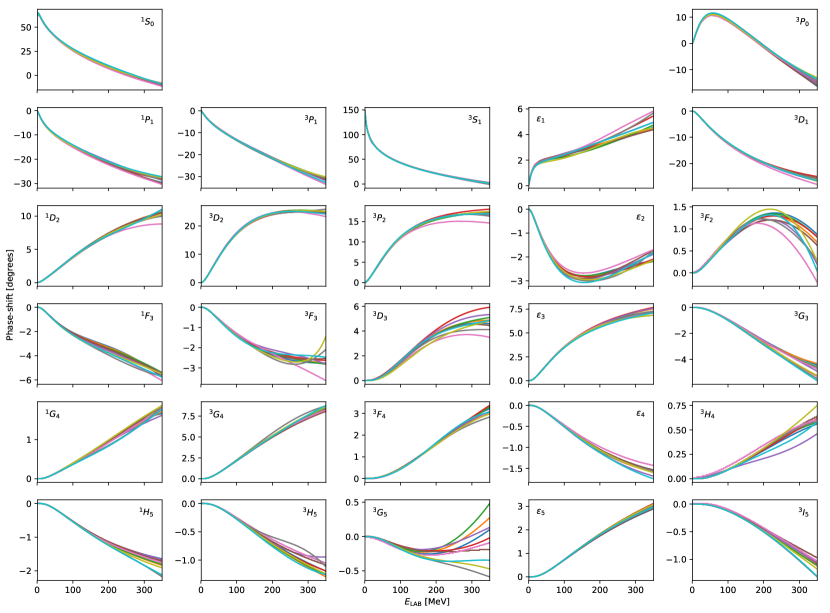
Figure 6: np Phase shifts for 10 high quality fits in all partial waves with $J\leq 5$ as a function of the LAB energy. We show the Nijmegen PWA  Nijm I, NijmII Reid93 Stoks:1994wp the AV18 Wiringa:1994wb , CD Bonn Machleidt:2000ge , Spectator Gross:2008ps , and the Granada DS-OPE Perez:2013mwa ; Perez:2013jpa , DS-$\chi$TPE Perez:2013oba ; Perez:2013cza and Gauss-OPE Perez:2014yla .

4.2 Fitting and selecting data

This approach allows to select the largest self-consistent existing NN database with a total of 6713 NN scattering data driven by the coarse grained potential Perez:2013jpa ; Perez:2014yla with the rewarding consequence that statistical uncertainties can confidently be propagated . Precise determinations of chiral coefficients, $c_{1},c_{3},c_{4}$ Perez:2014bua ; Perez:2013za , the isospin breaking pion-nucleon Perez:2016aol ; Arriola:2016hfi , and the pion-nucleon-delta Perez:2014waa coupling constants have been made.

One important aspect regards the correlation properties among the fitting parameters. In our case one gets for the potential components at the sampling points $r_{n}$ the values $V_{i}(r_{n})\pm\Delta V_{i}(r_{n})$. When going to the partial wave basis, $V_{l,l^{\prime}}^{JS}(r_{n})$ one observes that different partial waves are largely decorrelated Perez:2014yla ; Perez:2014kpa . This shows a posteriori that the assumption of independent parameters is somewhat confirmed. As a bonus, this lack of strong correlations allows in practice for a very efficient search of the minimum of the $\chi^{2}$.

4.3 Systematic vs Statistical errors

Our analysis has clearly demonstrated that at least the statistically validated 6-Granada potentials exhibit similar statistical errors but different most likely values of the predicted quantities Perez:2014waa . The most vivid example is provided by the phase shifts as we show in Fig. 6. We also plot in the figure the results for the previous high quality potentials at their time (defined by their $\chi^{2}/N\sim 1$). Our observation is that for the Granada potentials, which are statistically validated with the same Granada-2013 database, we have that if a phase-shift for potential $V^{(i)}$ in a given partial wave is $\delta^{(i)}\pm\Delta\delta_{\rm stat}^{(i)}$, then

$$\Delta\delta_{\rm stat}^{(1)}\sim\dots\sim\Delta\delta_{\rm stat}^{(6)}\,,$$ (48)

but the standard deviation defined as usual, obbeys

$$\Delta\delta_{\rm sys}\equiv{\rm Std}(\delta^{(1)},\dots,\delta^{(6)})\gg\Delta\delta_{\rm stat}^{(i)}\,.$$ (49)

In all cases the potential above $r=3$fm including CD-OPE and all electromagnetic effects are the same, thus the discrepancies between different forms of representing the potential at short distances dominate the uncertainties, rather than the np and pp experimental data themselves.

A way of comparing potentials which actually minimizes the role of short distances is by considering radial moments,

$$C_{n,i}\sim\int_{0}^{\infty}d^{3}rr^{n}V_{i}(r)$$ (50)

which correspond to a low momentum expansion of the potential in momentum space. The resulting values for all active channels have been found to be rather universal yet the larger systematic vs statistical uncertainties are also found Perez:2016vzj . This effect is also found in the low energy parameters characterizing low energy scattering, see Eq. (17), and the Wolfenstein parameters RuizSimo:2017anp .

5 The chiral potentials

In the previous sections we have reviewed some aspects needed in the construction of the Granada-2013 database. In the remaining sections we will compare the quality of the chiral approach on the light of these developments. We will try to check to what extent the chiral hierarchy complies with the trends observed in the NN data analysis in the last 26 years since the Nijmegen group first found a statistically satisfactory description of the data at the time with a large database.

5.1 Chiral counting

Despite the long discussions on the correctness and suitability of the Weinberg power counting, most applications to light nuclei use this scheme based on a NN potential in practice, and we will therefore restrict our short reminder to this very significant case. The Weinberg chiral counting relies on the heavy-baryon formalism and a naive dimensional analysis of the NN potential. Thus, according to the Feynman rules of covariant perturbation theory, a nucleon propagator is $Q^{-1}$, a pion propagator $Q^{-2}$, each derivative in any interaction is $Q$, each four-momentum integration $Q^{4}$ and the pion mass $m_{\pi}$ is also $Q$. In addition, for reasons explained in Ref. Weinberg:1990rz , terms including factors of $Q/M_{N}$, where $M_{N}$ denotes the nucleon mass are counted by the rule $Q/M_{N}\sim(Q/\Lambda_{\chi})^{2}$. There are two kinds of contributions for the total potential

$$V=V_{\rm ct}+V_{\pi}$$ (51)

where $V_{\pi}$ is the long range contributions containing an increasing number of pion exchanges,

$$V_{\pi}=V_{1\pi}+V_{2\pi}+V_{3\pi}+\ldots\,,$$ (52)

which are discontinuous function of the momentum transfer at $q=im_{\pi},2im_{\pi},3im_{\pi},\dots$ and $V_{\rm ct}$ are contact contributions which do not present this discontinuity and to a given order reduce to polynomials in initial and final momenta, $p$ and $p^{\prime}$ respectively,

$$V_{\rm ct}=V_{\rm ct}^{(0)}+V_{\rm ct}^{(2)}+V_{\rm ct}^{(4)}+V_{\rm ct}^{(6)}+\ldots\;,$$ (53)

where the superscript denotes the power or order and parity and time-reversal only allows even powers of momentum. Pion exchange terms, we have a similar expansion

$$V_{1\pi} =V_{1\pi}^{(0)}+V_{1\pi}^{(2)}+V_{1\pi}^{(3)}+V_{1\pi}^{(4)}+V_{1\pi}^{(5)}+\ldots$$ (54)

$$V_{2\pi} =V_{2\pi}^{(2)}+V_{2\pi}^{(3)}+V_{2\pi}^{(4)}+V_{2\pi}^{(5)}+\ldots$$ (55)

$$V_{3\pi} =V_{3\pi}^{(4)}+V_{3\pi}^{(5)}+\ldots\,,$$ (56)

Order by order, the complete $NN$ potential builds up as follows:

$$V_{\rm LO} =V_{\rm ct}^{(0)}+V_{1\pi}^{(0)}$$ (57)

$$V_{\rm NLO} =V_{\rm LO}+V_{1\pi}^{(2)}+V_{2\pi}^{(2)}+V_{\rm ct}^{(2)}$$ (58)

$$V_{\rm N2LO} =V_{\rm NLO}+V_{1\pi}^{(3)}+V_{2\pi}^{(3)}$$ (59)

$$V_{\rm N3LO} =V_{\rm N2LO}+V_{1\pi}^{(4)}+V_{2\pi}^{(4)}+V_{3\pi}^{(4)}+V_{\rm ct}^{(4)}$$ (60)

$$V_{\rm N4LO} =V_{\rm N3LO}+V_{1\pi}^{(5)}+V_{2\pi}^{(5)}+V_{3\pi}^{(5)}$$ (61)

where LO stands for leading order, NLO for next-to-leading order, etc.. From the point of view of the potential operators, Eq. (21), the chiral hierarchy reads

$$m_{\pi}^{2}W_{T} ={\cal O}(Q^{0})$$ (62)

$$V_{T},W_{C},V_{S} ={\cal O}(Q^{2})$$ (63)

$$V_{C},W_{S},m_{\pi}^{2}V_{SL},m_{\pi}^{2}W_{SL} ={\cal O}(Q^{3})$$ (64)

$$m_{\pi}^{4}V_{Q} ={\cal O}(Q^{5})$$ (65)

$$m_{\pi}^{4}W_{Q},m_{\pi}^{2}V_{P},m_{\pi}^{2}W_{P} \leq{\cal O}(Q^{6})$$ (66)

where we have multiplied by a power of $m_{\pi}$ so that all components have the same dimensions.

It is noteworthy that the central force, traditionally taken as the main contribution to the mid range attraction which holds atomic nuclei together, rather than being LO becomes N2LO in the chiral expansion. Moreover, we would need to go at least to order ${\cal O}(Q^{7})$ or higher, to generate a term $W_{Q}$. We will see later on that the phenomenological approaches require a non-vanishing and statistically significant $|W_{Q}|\gg\Delta W_{Q}$.

The size of the potential is relevant to discuss the chiral hierarchy, but it is unclear how this could be done quantitatively. One may, for instance, compare local potentials at a fixed distance, but the question ambiguity remains as the question of what is a reasonable distance to compare?. Field theoretical potentials diverge at short distances and they even make the quantum mechanical problem mathematically ill defined. The separation distance between the explicit pion exchange and the unknown part of the nuclear potential plays the role of a cut-off in coordinate space. We believe that the comparison of the local components of potentials as a function of the momentum transfer made in Fig. 5 goes more to the point. These components can be related to the contributions displayed in Eq. (21) by the relations in the Appendix A. In fairness the comparison should be made for small $q$ values (typically $\sim m_{\pi}$). The central component makes a large variation from this range where it is small to a large value for $q\sim 3{\rm fm}^{-1}\sim 4m_{\pi}$. This is in agreement with the chiral suppression and the phenomenology on the dominance of the mid-range central force. At small q the largest component is by far the tensor force as implied also by the chiral counting.

5.2 Scale dependence and the number of parameters

The short range components of the NN potentials depend on the maximal fitting energy (see e.g. Ref. NavarroPerez:2013iwa for an explicit example). This is not so often realized because the maximal fitting energy is usually fixed to a conventional value, usually $T_{\rm LAB}\leq 350$MeV. If we take $\Lambda=p_{\rm CM}^{\rm max}$, the LS equation at the partial waves level reads,

$$T_{l^{\prime}l}^{JS}(p^{\prime},p) = V_{l^{\prime}l}^{JS}(p^{\prime},p)$$ (67)

$$+ \frac{2}{\pi}\sum_{l^{\prime\prime}}\int_{0}^{\Lambda}dqV_{ll"}^{JS}(p^{\prime},q)\frac{q^{2}}{k^{2}-q^{2}}T_{l^{\prime\prime},l}^{JS}(q,p)\,$$

In a loose sense, the contact pieces in the chiral potentials represent the role of counter-terms in quantum field theory, but their significant value depends on $\Lambda$. For small momenta one has

$$V_{l^{\prime},l}^{JS}(p^{\prime},p)|_{ct}=(p^{\prime})^{l^{\prime}}p^{l}\sum_{n,m=0}^{\infty}C_{nm}(\Lambda)(p^{\prime})^{2n}p^{2m}$$ (68)

where $C_{nm}=C_{mn}$ are real. In the limit, $\Lambda\to 0$, their values may be directly computed from the low energy threshold parameters RuizArriola:2016vap only up to ${\cal O}(p^{2})$. For higher orders, there are more counter-terms than threshold parameters, featuring again in the low energy limit the ambiguity of the inverse scattering problem. Some ambiguity can be shifted by performing a suitable unitary transformation as, for instance, discard purely off-shell contributions Reinert:2017usi in which case to ${\cal O}(p^{2n})$ the number of parameters would be $N_{\rm Par}=(4+5n)(n+1)/2=2,9,21,38,60,\dots$ for $n=0,1,2,3,4,\dots$ PavonValderrama:2005ku .

5.3 Chiral potential fits to NN scattering data

While the most portable form of a PWA corresponds to listing the phase shifts and this clearly provides a very reasonable picture of the scattering process, from the point of view of validation/falsification of the interaction fitting phase-shifts and fitting scattering data are quite different. Therefore we will only consider chiral fits to a full database containing cross sections and polarization observables. The first chiral fits using the N2LO chiral potentials Kaiser:1997mw to the Nijmegen database were undertaken by the Nijmegen group itself for pp Rentmeester:1999vw and for pp+np Rentmeester:2003mf , allowing for a determination of the chiral constants $c_{1},c_{3},c_{4}$. The newest generation of chiral potentials provide fits to the Granada-2013 database Perez:2013oba ; Perez:2013cza ; Perez:2014bua ; Carlsson:2015vda ; Piarulli:2016vel ; Reinert:2017usi ; Entem:2017gor . The best fit we have obtained provides $\chi^{2}/\nu=1.025$ when isospin breaking is incorporated both in the pion masses, the coupling constants and in the short range contribution Perez:2016aol ; Arriola:2016hfi .

The recent calculations by the Idaho-Salamanca group Entem:2017gor and the Bochum group Reinert:2017usi , are possibly the most complete analyses to date of chiral potentials going up to N4LO in the Weinberg counting which basically use the Granada 2013 database which contains $N_{\rm Dat}=2996_{pp}+3717_{np}=6713$ data which are $3\sigma$ mutually compatible by a coarse grained potential with $\chi^{2}/\nu=1.027$. The fact that both groups take $T_{\rm LAB}\lesssim 290-300$MeV and that they thus have about $N_{\rm Dat}\sim 4850$ implies that a fit would be satisfactory a posteriori if $\chi^{2}/N_{\rm Dat}=1\pm 0.02$. Our discussion below adopts this point of view.

One remarkable aspect of the Bochum analysis Reinert:2017usi is the fact that they show that for the first time the chiral potential fit outperforms the traditional potentials such as those of the Nijmegen group and AV18 with much less parameters when the Granada-2013 database is taken. In both Idaho-Salamanca and Bochum cases cases a relevant (Gaussian) regulator dependence in the quality of the fit in the “reasonable” range $\Lambda\sim 450-550$MeV is reported. Likewise, a systematic order by order analysis seems to indicate convergence of the chiral approach.

In the Idaho-Salamanca study a N4LO nonlocal potential is used to fit $N_{\rm Dat}=4853$-NN data are analyzed below $T_{\rm LAB}=290$MeV. The quality of such a fit is not given, but they quote the results for the N4LO⁺ consisting in the addition of additional counter-terms in the F-waves, which are nominally N5LO, but disregarding the presumably small pion contributions $V_{\pi}^{(6)}$,

$$V_{{\rm N4LO}^{+}}\equiv V_{\rm N4LO}+V_{\rm ct}^{(6)}$$ (69)

obtaining in this case a total best fit value $\chi^{2}/N_{\rm Dat}=1.15$ when 148 np data (Granada-accepted by the $3\sigma$ criterion) are replaced by 140 pp data (Granada-rejected by the $3\sigma$ criterion). Likewise, the Bochum group uses a semi-local N4LO chiral potential and analyze a total of $N_{\rm Dat}=4855$-NN data are analyzed below $T_{\rm LAB}=300$MeV with a best $\chi^{2}/N_{\rm Dat}=1.39$. Only after some (Granada accepted) data are removed and adding also F-waves counter-terms, thus working in the N4LO⁺ scheme, they get $\chi^{2}/N_{\rm Dat}=1.03$ which is very good. From this we may infer that the effect of going from N4LO to (incomplete) N4LO⁺ is crucial for claiming that the chiral expansion has converged.

We believe that this selected but different exclusion best exemplifies the main difference between power counting and the coarse graining approach used to fix the Granada-2013 database. Of course, it would be highly desirable to go to the next order and check if the problem could be solved. An approximate way of doing this would be to include the G-waves counter-terms in a N4LO⁺⁺ scheme.

To summarize, both calculations are nominally N4LO but the quality of the fits only gets improved when F-wave counter-terms are added when $T_{\rm LAB}\lesssim 290-300$MeV, the so-called N4LO⁺, which indicate a flagrant violation of the standard Weinberg power counting unless it is shown the $V_{\pi}^{(6)}$ is significantly negligible. Another possibility is to reduce the energy, so that F-wave counter-terms become marginal. We comment this possibility below in Sect. 6.3.

As it has been emphasized over the years by their own practitioners the raison d’être of the EFT approach lies in the systematic determination of the physical observables in a power counting scheme. Taken at face value, the quoted values of the $\chi^{2}/\nu$ are several $\sigma$’s away from their expected values, showing that the chiral N4LO⁺ potentials despite violating the chiral counting, are still incompatible with the existing data. The quality of the fits in the N4LO⁺ case, supports their use in nuclear physics as valid representations of the NN scattering data below $T_{\rm LAB}=290-300$MeV, but not more than say any of the previous high quality potentials since the 1993 Nijmegen analysis.

In our works Perez:2014yla ; Perez:2014kpa (see also Perez:2015pea for a $\pi\pi$ based presentation), we have insisted on the fact that if $\chi^{2}/\nu$ is not within the expected values, one can still slightly scale the errors by the so-called Birge factor provided one can show that the residuals are still a scaled Gaussian distribution with a variety of statistical normality tests based in an analysis of the tails or the moments of the distribution of residuals. For instance, for $\nu=7000$ one should have $\chi^{2}/\nu=1\pm 0.017$. Having instead, $\chi^{2}/\nu=1.08$ would mean $5\sigma$ incompatible fit. However, if the normality test is passed it is plausible that the rescaling of the $\chi^{2}$ corresponds to a rescaling of the data uncertainties by only 10$\%$ factor, fully compatible with the “error on the error”. We of course, should not exclude the interesting possibility that the N4LO analyses themselves pass the normality tests and thus qualify as suitable description of NN scattering data.

Table 1: The pion-nucleon coupling constant $f^{2}=f_{p}^{2}=f_{0}^{2}=f_{c}^{2}$ and the chiral constants $c_{1}$, $c_{3}$ and $c_{4}$ determined from different fits to the Granada-2013 database and of the CD-OPE plus $\chi$TPE potential depending on the cut-off radius $r_{c}$. Charge dependence is only allowed on the ${}^{1}S_{0}$ partial wave. Here we take $T_{\rm LAB}\leq 350{\rm MeV}$ and define $N_{\sigma}=(\chi^{2}/\nu-1)/\sqrt{2/\nu}$.

$r_{c}({\rm fm})$	$f^{2}$	$c_{1}({\rm GeV}^{-1})$	$c_{3}({\rm GeV}^{-1})$	$c_{4}({\rm GeV}^{-1})$	$\chi^{2}_{pp}$	$\chi^{2}_{np}$	$\chi^{2}$	$N_{\rm Dat}$	$N_{\rm Par}$	$\chi^{2}/\nu$	$N_{\sigma}$
3.6	$0.075$	$1010.0(306)$	$-990.9(264)$	$9.6(140)$	2975.09	3879.15	6854.24	6719	63	1.030	1.7
3.6	$0.0710(6)$	$978.3(390)$	$-961.1(353)$	$-4.0(148)$	2965.28	3869.62	6834.90	6719	64	1.027	1.6
3.0	$0.075$	$-44.4(70)$	$39.5(51)$	$-4.4(26)$	2979.46	3980.27	6959.73	6721	49	1.043	2.5
3.0	$0.0763(3)$	$-35.2(79)$	$31.3(60)$	$-6.4(27)$	2983.95	3968.28	6952.23	6721	50	1.042	2.4
2.4	$0.075$	$-10.6(18)$	$5.2(10)$	$-2.1(8)$	3064.38	4049.88	7114.26	6718	41	1.065	3.8
2.4	$0.0748(2)$	$-11.9(20)$	$6.0(12)$	$-2.3(9)$	3065.80	4048.30	7114.11	6718	42	1.066	3.8
1.8	$0.075$	$-1.9(6)$	$-3.7(2)$	$4.4(2)$	3101.24	4059.32	7160.56	6717	33	1.071	4.1
1.8	$0.0763(2)$	$-1.6(6)$	$-3.7(3)$	$4.3(2)$	3077.00	4050.22	7127.22	6717	34	1.066	3.8
1.2	$0.075$	$-11.17(9)$	$0.76(2)$	$2.822(2)$	3428.38	4659.52	8087.90	6715	25	1.209	12.1
1.2	$0.07500(3)$	$-11.17(9)$	$0.76(3)$	$2.821(6)$	3428.28	4659.02	8087.31	6715	26	1.209	12.1

5.4 N5LO chiral forces

The chiral expansion provides a hierarchy in the components of the NN interaction. Can we check this hierarchy by just analyzing NN scattering data directly?. We feel that this is rather difficult, however, we can instead check whether the chiral pattern is verified for potential models. In the Weinberg counting to sixth order (N5LO ) one finds that the component $W_{Q}=0$ whereas one has $V_{Q}={\cal O}(1/f^{4}M_{N}^{2})$ Kaiser:2001at . If the chiral expansion would have converged to that order one should see that this component is actually very much suppressed in the phenomenological analysis of NN scattering data. The results presented in Fig. 5 show that this is not the case. As we see, the contribution to $W_{Q}$ (proportional to $V_{14a}$, see Appendix A) which vanishes for ChPT to N5LO is not vanishing within uncertainties. Thus, this is a serious indication that one has still to go higher orders to accommodate the non-vanishing value character of all NN potential components.

Finally, we remind that Eq. (9) does not hold off-shell but to N5LO $V_{P}=W_{P}=0$. Such a dependence appears when considering $A_{1}$ exchange to ${\cal O}(1/M_{N}^{2})$. Taking into account that the quantum numbers of $A_{1}$ are the same as $3\pi$ (The decay process $A_{1}\to\rho\pi\to(\pi\pi)\pi$ is the dominant mechanism ) and that there are $3\pi$ exchange contributions to N5LO some clarification would be needed to explain to what order does one expect a non-vanishing of $V_{P}$ and $W_{P}$.

Table 2: Fits of the $\chi$-TPE potentials depending on the cutoff radius and the maximum fitting energy as described in Perez:2013za . The chiral constants of the fourth line were taken from a Ref. Ekstrom:2013kea ; Ekstrom:2014dxa and used as fixed values during the $\chi^{2}$ minimization with respect of the delta-shell parameters. Highest counter-term column indicates the maximum angular momentum where at least one delta-shell strength coefficient is non-vanishing.

Max $T_{\rm LAB}$	$r_{c}$	$c_{1}$	$c_{3}$	$c_{4}$	Highest	$\chi^{2}/\nu$
MeV	fm	GeV-1	GeV-1	GeV-1	counter-term
350	1.8	$-0.4(11)$	$-4.7(6)$	$4.3(2)$	$F$	1.08
350	1.2	$-9.8(2)$	$0.3(1)$	$2.84(5)$	$F$	1.26
125	1.8	$-0.3(29)$	$-5.8(16)$	$4.2(7)$	$D$	1.03
125	1.2	$-0.92$	$-3.89$	$4.31$	$P$	1.70
125	1.2	$-14.9(6)$	$2.7(2)$	$3.51(9)$	$P$	1.05

6 Chiral Miscellany and loose ends

6.1 Naturalness

While the statistical approach to NN is based on a standard least squares optimization, which minimizes the distance between the theory and the experiment for many pp and np scattering data, it is important to underline that not all fits are eligible and in fact some of them should be rejected, either because they generate spurious bound states or because some of the fitting parameters turn out to be rather different than grounded theoretical expectations.

In the case of $\chi$TPE exchange, the chiral constants $c_{1,3,4}$ are saturated by meson exchange Bernard:1996gq . Actually, $c_{1}$ is saturated by scalar exchange $c_{1}^{S}=-g_{S}c_{m}/m_{S}^{2}$. Taking $M_{N}=g_{S}F_{\pi}$ and $c_{m}=F_{\pi}/2$ , $m_{S}=m_{V}=F_{\pi}\sqrt{24\pi/N_{c}}$ and $M_{N}=N_{c}m_{\rho}/2$ Ledwig:2014cla we get $c_{1}^{S}\sim-N_{c}/(4\sqrt{2}m_{\rho})\sim-0.7{\rm GeV}^{-1}$ and $c_{3}$ and $c_{4}$ are saturated by $\Delta$ resonance; taking $\Delta=M_{\Delta}-M_{N}$ one has $c_{2}^{\Delta}=-c_{3}^{\Delta}=2c_{4}^{\Delta}=g_{A}^{2}/(2\Delta)\sim 2.97{\rm GeV}^{-1}$. Of course, these are not very accurate values, but indicate the order of magnitude one should expect.

The results in Table 1 illustrate this point when the $\chi$TPE (N2LO) potential is used to fit the Granada-2013 database and the chiral constants $c_{1,3,4}$ are taken as fitting parameters. As we see, the best fit does not produce natural values for $c_{1,3,4}$ and hence should be rejected. The natural values correspond to the cut-off distance $r_{c}=1.8-2.4{\rm fm}$. The table also illustrates that the small cut-off $r_{c}=1.2{\rm fm}$ is incompatible with the data. From the point of view of the effective elementarity of the nucleon, where $r_{e}=1.8$fm, the value $r_{c}=1.8$fm is the smallest possible and hence provides the minimal number of parameters, which for pn+pp turns out to be about $N_{\rm Par}=30$ when $T_{\rm LAB}\leq 350$MeV.

6.2 Power counting vs Coarse graining

We want to elaborate on the main differences between power counting and coarse graining. As mentioned before, in the partial wave amplitude we have a left-hand branch cuts due to multiple $n-\pi$ exchanges, $p,p^{\prime}=inm_{\pi}/2$ Thus, in a low momentum expansion corresponding to $|p|,|p^{\prime}|<m_{\pi}/2$ we have a Taylor expansion as in Eq. (68), but the coefficients are functions of $m_{\pi}$. If we count powers of $Q=p,p^{\prime},m_{\pi}$ we have further the expansion

$$C_{0}(m_{\pi}^{2})=c_{0}+c_{0}^{\prime}m_{\pi}^{2}+\dots$$ (70)

Already at this level we see the phenomenon of parameter redundancy; in a combination such as $c_{0}+c_{0}^{\prime}m_{\pi}^{2}+\dots$ the constants $c_{0}$, $c_{0}^{\prime}$, etc. cannot be disentangled from NN data. As a general rule, the number of parameters of the pion-less theory is smaller than the pion-full theory, since the pion exchange potentials also contain LEC’s (stemming e.g. from $\pi N$ scattering). Thus, while a power counting scheme the total number of parameters depends on the the maximal energy and the accuracy of the experimental data, in the coarse graining scheme the number of parameters is essentially limited by the maximal fitting energy, see Eq. (33), fixing the discernible wavelength resolution.

6.3 The short distance cut-off

The questions on the numerical cut-of $r_{c}$ supported by the analysis of data can be resolved by explicitly separating the potential as indicated by Eq. (32) and changing the maximal fitting energy. The results checked to be statistically consistent in  Perez:2013za are summarized in Table 2. It is striking that $D$-waves, nominally N3LO and forbidden by Weinberg chiral counting at N2LO, are indispensable !. Furthermore, data and N2LO do not support $r_{c}<1.8{\rm fm}$, while several $\chi$-potentials Gezerlis:2014zia ; Piarulli:2014bda take $r_{c}=0.9-1.1{\rm fm}$ as “reasonable”. This need of higher order counter-terms is also found in more complete and higher order calculations , where $F$-waves (N5LO) counter-terms are added despite keeping the pion exchange contribution to one lower order.

Of course, one may think that 125 MeV is too large an energy. We find that when we go down to 40 MeV, the $\chi$TPE potential becomes invisible being compatible with zero within statistical uncertainties from the experimental data Amaro:2013zka ; Perez:2013cza .

The chiral potential (including $\Delta$-degrees of freedom) of Ref. Piarulli:2014bda explicitly violates Weinberg’s counting since it has N2LO long distance and N3LO short distance pieces, and residuals are not Gaussian. More recently, the local short distance components of this potential have been fitted up to 125 MeV LAB energy Piarulli:2016vel improving the goodness of the fit, similarly to Perez:2013za (see also table 2). As already said, the most recent and improved N4LO chiral potentials by Idaho-Salamanca Entem:2017gor and the Bochum Reinert:2017usi groups suffer also from this deficiency although the order mismatch is displaced to higher orders. In both cases, a substantial improvement is achieved by introducing F-wave counter-terms, which properly speaking are N5LO.

6.4 The deconstruction argument

An alternative way of checking the failure of the power counting is provided by a deconstruction argument Perez:2013za . This corresponds to determine under what conditions are the short distance phases $\delta_{\rm short}$, .i.e. the phase shifts stemming solely from $V_{\rm short}$ compatible with zero within uncertainties, i.e. $|V_{\rm short}|<\Delta V$ ?. This is equivalent to determine what partial waves fulfill $|\delta_{\rm short}|\leq\Delta\delta_{\rm stat}$ when $r_{c}=1.8\,{\rm fm}$. Unfortunately, this does not work for D-waves, when the fit to 125 MeV is undertaken, in full agreement with the previous conclusions.

6.5 The impact parameter argument

The long distance character of $\chi$TPE makes peripheral phases (large angular momentum) to be suitable for a perturbative comparison without counter-terms Kaiser:1997mw ; Kaiser:1998wa ; Entem:2014msa . However, one should take into account that 1) peripheral phases can only be obtained from a complete phase shift analyses and 2) their uncertainties are tiny Perez:2013jpa . The analysis of Entem:2014msa just makes an eyeball comparison which looks reasonable but the agreement was not quantified. A careful comparison reflects that the thickness of their points in their figures are much larger than the estimated errors from high quality fits. We find that peripheral waves predicted by 5th-order chiral perturbation theory are not consistent with the Granada-2013 self-consistent NN database RuizSimo:2017anp . A very vivid way of presenting the discrepancy is by comparing the phase-shifts in terms of the impact parameter, defined as

$$b=(L+\frac{1}{2})/p$$ (71)

and the variable for every partial wave

$$\xi^{\rm N4LO}=\frac{\delta^{\rm N4LO}-{\rm Mean}(\delta)}{{\rm Std}(\delta)}\,,$$ (72)

which measures the deviation from the phase-shift corresponding to the N5LO phases to the averaged phase-shift divided by its standard deviation. The conclusions of Ref. RuizSimo:2017anp are that for $2{\rm fm}\leq b\leq 5{\rm fm}$, one has $\xi^{\rm N4LO}\sim 5$ for the Granada PWA, $\xi^{\rm N4LO}\sim 3$ for the 6 Granada potentials, $\xi^{\rm N4LO}\sim 1$ for the 13 high quality potentials. Our interpretation of this result is that the systematic error of the perturbative N5LO reflects the variations of the peripheral phases in the last 26 years.

$$\Delta\delta^{\rm PWA,syst}\sim|\delta^{\chi{\rm,N4LO}}-\delta^{\rm PWA}|\gg\Delta\delta^{\rm PWA,stat}\,.$$ (73)

Sometimes we get even $3\sigma$ discrepancies. More details on this peripheral analysis are presented in Ref. RuizSimo:2017anp .

Table 3: Low energy threshold np parameters for all partial waves with $2\leq j\leq 5$. The central value and statistical error bars are given on the first line using the DS-OPE potential Perez:2013mwa ; Perez:2013jpa . The second line quotes the systematic uncertainties, the central value and error bars correspond to the mean and standard deviation of the 6 realistic potentials NijmII Stoks:1994wp , Reid93 Stoks:1994wp , AV18 Wiringa:1994wb , DS-OPE Perez:2013mwa ; Perez:2013jpa , DS-$\chi$TPE Perez:2013oba ; Perez:2013cza and Gauss-OPE Perez:2014yla . The third line is the N2LO perturbative $\chi$PT result with OPE (charge independent with $f_{\pi NN}^{2}=0.075$ and $m_{\pi}=(m_{\pi^{0}}+2m_{\pi^{+}})/3$) and $\chi$TPE potentials. For each partial wave we show the scattering length $\alpha$ and the effective range $r_{0}$, both in ${\rm fm}^{l+l^{\prime}+1}$, as well as the curvature parameters $v_{2,3,4}$ in ${\rm fm}^{l+l^{\prime}+3,5,7}$. For the coupled channels we use the nuclear bar parameterization of the $S$ matrix. Uncertainties smaller than $10^{-3}$ are not quoted

Wave	${\rm Scheme}$	$\alpha$	$r_{0}$	$v_{2}$	$v_{3}$	$v_{4}$
${}^{1}D_{2}$	${\rm PWA}_{\rm stat}$	$-1.376$	$15.04(2)$	$16.68(6)$	$-13.5(1)$	$35.4(1)$
	${\rm PWA}_{\rm syst}$	$-1.380(7)$	$15.0(1)$	$16.6(2)$	$-13.1(3)$	$36.1(16)$
	${\rm N2LO}_{\rm pert}$	$-1.768$	$12.81$	$12.92$	$-18.36$	$-3.602$
${}^{3}D_{2}$	${\rm PWA}_{\rm stat}$	$-7.400(4)$	$2.858(3)$	$2.382(9)$	$-1.04(2)$	$1.74(2)$
	${\rm PWA}_{\rm syst}$	$-7.40(1)$	$2.861(8)$	$2.40(2)$	$-0.98(3)$	$1.8(1)$
	${\rm N2LO}_{\rm pert}$	$-7.564$	$2.784$	$2.323$	$-0.931$	$1.775$
${}^{3}P_{2}$	${\rm PWA}_{\rm stat}$	$-0.290(2)$	$-8.19(1)$	$-6.57(5)$	$-5.5(2)$	$-12.2(3)$
	${\rm PWA}_{\rm syst}$	$-0.287(6)$	$-8.2(2)$	$-6.6(7)$	$-5.3(18)$	$-11.7(24)$
	${\rm N2LO}_{\rm pert}$	$1.028$	$-3.346$	$4.157$	$-3.359$	$-11.56$
$\epsilon_{2}$	${\rm PWA}_{\rm stat}$	$1.609(1)$	$-15.68(2)$	$-24.91(8)$	$-21.9(3)$	$-64.1(7)$
	${\rm PWA}_{\rm syst}$	$1.607(6)$	$-15.7(2)$	$-25.0(7)$	$-21.9(30)$	$-63.6(69)$
	${\rm N2LO}_{\rm pert}$	$2.039$	$-6.480$	$-0.457$	$13.02$	$-43.64$
${}^{3}F_{2}$	${\rm PWA}_{\rm stat}$	$-0.971$	$-5.74(2)$	$-23.26(8)$	$-79.5(4)$	$-113.0(16)$
	${\rm PWA}_{\rm syst}$	$-0.970(5)$	$-5.7(1)$	$-23.1(6)$	$-79.0(35)$	$-113.0(129)$
	${\rm N2LO}_{\rm pert}$	$-1.371$	$7.416$	$24.53$	$49.59$	$-37.49$
${}^{1}F_{3}$	${\rm PWA}_{\rm stat}$	$8.378$	$-3.924$	$-9.869(4)$	$-15.27(2)$	$-1.95(7)$
	${\rm PWA}_{\rm syst}$	$8.376(7)$	$-3.927(5)$	$-9.89(3)$	$-15.4(2)$	$-2.3(4)$
	${\rm N2LO}_{\rm pert}$	$8.531$	$-3.836$	$-9.620$	$-14.75$	$-1.51$
${}^{3}F_{3}$	${\rm PWA}_{\rm stat}$	$2.689$	$-9.978(3)$	$-20.67(2)$	$-19.12(8)$	$-27.7(2)$
	${\rm PWA}_{\rm syst}$	$2.692(7)$	$-9.97(3)$	$-20.6(1)$	$-19.0(4)$	$-27.0(7)$
	${\rm N2LO}_{\rm pert}$	$3.779$	$-8.142$	$-18.25$	$-21.34$	$-0.773$
${}^{3}D_{3}$	${\rm PWA}_{\rm stat}$	$-0.134$	$1.373$	$2.082(3)$	$1.96(1)$	$-0.45(3)$
	${\rm PWA}_{\rm syst}$	$-0.15(2)$	$1.370(3)$	$2.07(2)$	$1.91(7)$	$-0.5(1)$
	${\rm N2LO}_{\rm pert}$	$-0.228$	$1.330$	$1.986$	$1.768$	$-0.857$
$\epsilon_{3}$	${\rm PWA}_{\rm stat}$	$-9.682$	$3.262$	$7.681(3)$	$9.62(2)$	$-1.09(5)$
	${\rm PWA}_{\rm syst}$	$-9.684(6)$	$3.258(5)$	$7.66(3)$	$9.5(1)$	$-1.2(2)$
	${\rm N2LO}_{\rm pert}$	$-9.847$	$3.170$	$7.39$	$8.79$	$-2.61$
${}^{3}G_{3}$	${\rm PWA}_{\rm stat}$	$4.876$	$-0.027$	$0.019(2)$	$0.07(1)$	$-2.69(3)$
	${\rm PWA}_{\rm syst}$	$4.875(3)$	$-0.04(1)$	$-0.03(6)$	$-0.2(3)$	$-3.1(6)$
	${\rm N2LO}_{\rm pert}$	$4.941$	$-0.084$	$-0.342$	$-2.18$	$-9.89$
${}^{1}G_{4}$	${\rm PWA}_{\rm stat}$	$-3.208$	$10.833(1)$	$34.629(9)$	$83.04(8)$	$108.1(4)$
	${\rm PWA}_{\rm syst}$	$-3.213(8)$	$10.81(2)$	$34.54(8)$	$82.5(4)$	$106.1(17)$
	${\rm N2LO}_{\rm pert}$	$-5.177$	$7.889$	$27.79$	$77.233$	$66.44$
${}^{3}G_{4}$	${\rm PWA}_{\rm stat}$	$-19.145$	$2.058$	$6.814$	$16.769(4)$	$10.00(2)$
	${\rm PWA}_{\rm syst}$	$-19.15(1)$	$2.058(1)$	$6.814(4)$	$16.78(2)$	$10.05(7)$
	${\rm N2LO}_{\rm pert}$	$-19.409$	$2.020$	$6.672$	$16.406$	$9.85$
${}^{3}F_{4}$	${\rm PWA}_{\rm stat}$	$-0.006$	$-3.043$	$-4.757(1)$	$73.903(5)$	$662.21(9)$
	${\rm PWA}_{\rm syst}$	$-0.009(3)$	$-3.040(8)$	$-4.75(5)$	$74.0(4)$	$662.5(40)$
	${\rm N2LO}_{\rm pert}$	$-0.0136$	$-2.504$	$-7.15$	$-14.03$	$-4.24$
$\epsilon_{4}$	${\rm PWA}_{\rm stat}$	$3.586$	$-9.529$	$-37.02(3)$	$-184.40(2)$	$-587.28(9)$
	${\rm PWA}_{\rm syst}$	$3.590(9)$	$-9.53(2)$	$-37.02(7)$	$-184.5(3)$	$-586.4(19)$
	${\rm N2LO}_{\rm pert}$	$5.783$	$-6.954$	$-23.92$	$-64.11$	$-53.56$
${}^{3}H_{4}$	${\rm PWA}_{\rm stat}$	$-1.240$	$-0.157(2)$	$-1.42(1)$	$-14.0(1)$	$-99.0(9)$
	${\rm PWA}_{\rm syst}$	$-1.241(4)$	$-0.17(1)$	$-1.51(9)$	$-14.9(9)$	$-105.4(59)$
	${\rm N2LO}_{\rm pert}$	$-2.351$	$-0.108$	$-1.088$	$-8.58$	$-30.63$
${}^{1}H_{5}$	${\rm PWA}_{\rm stat}$	$28.574$	$-1.727$	$-7.906$	$-32.787$	$-59.361$
	${\rm PWA}_{\rm syst}$	$28.58(2)$	$-1.727$	$-7.905(4)$	$-32.78(2)$	$-59.38(6)$
	${\rm N2LO}_{\rm pert}$	$28.830$	$-1.701$	$-7.758$	$-32.09$	$-58.03$
${}^{3}H_{5}$	${\rm PWA}_{\rm stat}$	$6.081$	$-6.439$	$-25.228$	$-82.511(3)$	$-168.47(2)$
	${\rm PWA}_{\rm syst}$	$6.09(2)$	$-6.43(2)$	$-25.21(6)$	$-82.5(1)$	$-168.1(9)$
	${\rm N2LO}_{\rm pert}$	$11.53$	$-4.135$	$-18.10$	$-70.12$	$-112.1$
${}^{3}G_{5}$	${\rm PWA}_{\rm stat}$	$-0.008$	$0.481$	$1.878$	$6.100$	$6.791$
	${\rm PWA}_{\rm syst}$	$-0.010(2)$	$0.480$	$1.878(1)$	$6.098(4)$	$6.78(1)$
	${\rm N2LO}_{\rm pert}$	$-0.009$	$0.471$	$1.837$	$5.958$	$6.63$
$\epsilon_{5}$	${\rm PWA}_{\rm stat}$	$-31.302$	$1.556$	$6.995$	$28.179$	$48.376(2)$
	${\rm PWA}_{\rm syst}$	$-31.31(2)$	$1.556$	$6.993(4)$	$28.17(1)$	$48.35(3)$
	${\rm N2LO}_{\rm pert}$	$-31.581$	$1.533$	$6.863$	$27.58$	$47.29$
${}^{3}I_{5}$	${\rm PWA}_{\rm stat}$	$10.678$	$0.011$	$0.146$	$1.441$	$6.546(6)$
	${\rm PWA}_{\rm syst}$	$10.680(6)$	$0.011$	$0.144(1)$	$1.43(2)$	$6.5(1)$
	${\rm N2LO}_{\rm pert}$	$10.711$	$0.010$	$0.143$	$1.41$	$6.35$

6.6 Threshold parameters at N2LO: Perturbative vs Non-perturbative

If chiral perturbation theory works for NN, the best scenario to check it is, as already mentioned, by looking at long distance properties, namely large angular momenta and small energies. This comparison provides a stringent test on the quality of chiral potentials. To this end we use the effective range expansion of the inverse amplitude generalized to higher partial waves including coupled channels, see, Eq. (17), going to ${\cal O}(p^{8})$. Practical formulas for the low energy threshold parameters have been deduced some time ago for the NijmII and Reid93 potentials PavonValderrama:2005ku and extended more recently for the set of 6 Granada potentials RuizSimo:2017anp using a discretized form of the variable phase approach of Calogero calogero_Variable_1967 .

We can illustrate the perturbative character of peripheral waves by comparing the low energy parameters, computed in chiral perturbation theory by using the N2LO TPE as a reference. This has the additional advantage that due to the angular momentum suppression there is a large insensitivity to the short distances so that the limit $r_{c}\to 0$ can be safely taken. However, it was shown in Ref. PavonValderrama:2005uj that due to the short distance singularities of the chiral potentials, see Eq. (5), there is a finite order in perturbation theory where regardless of the angular momentum the result is divergent. Possibly the most direct way to approach the calculation in perturbation theory is via the variable phase approach. Analytical formulas can be obtained but they are too lengthy to be quoted here, so we just give the final outcome and comment it. For the N2LO TPE potential the first perturbative calculable partial waves are D-waves, and for increasing F-,G-,H-, etc. partial waves we expect a faster convergence. In Table 3 we show the results when we take the central values of the chiral constants found in our previous work Perez:2013oba . As we generally see from a dedicated inspection of the table, while the perturbative numbers get closer to the full result for increasing angular momentum, including the systematic spread of the 6 Granada potentials, there is still a significant discrepancy due to the finite order of the perturbation. We remind that the same N2LO TPE used above $r_{c}=1.8$fm to all orders together with a delta-shells potential yields a satisfactory description of full Granada-2013 database.

6.7 Counter-terms vs Renormalization conditions: The zero energy argument

The low energy threshold parameters allow to probe the structure of chiral potentials against the NN interaction. The current approach to chiral interactions is to incorporate the $\chi$TPE tail and include short range counter-terms fitted to pp and np phase-shifts or scattering data Ekstrom:2013kea ; Ekstrom:2014dxa . However, these approaches are subject to strong systematic uncertainties since a fit to phase-shifts may be subjected to off-shell ambiguities and so far low energy chiral potentials fitted to data have not achieved Gaussian residuals Ekstrom:2014dxa or even have huge Gezerlis:2014zia to moderate Piarulli:2014bda $\chi^{2}/\nu$ values. To avoid these shortcomings we use $\chi$TPE Perez:2013oba ; Perez:2013cza with a simpler short range structure inferred from low energy threshold parameters Perez:2014waa with their uncertainties inherited from the 2013-Granada fit Perez:2013jpa . This corresponds to zero energy renormalization condition of the counter-terms.

One could naively expect to be able to set any number of short range counter-terms to reproduce the same number of low energy threshold parameters. Actually, in order to have the 9 counter-terms dictated by Weinberg to N2LO as in Ekstrom:2013kea we need to fix $\alpha_{0}$ and $r_{0}$ for both ${}^{1}S_{0}$ and ${}^{3}S_{1}$ waves, the mixing $\alpha_{\epsilon}$ and $\alpha_{1}$ for the ${}^{3}P_{0}$, ${}^{3}P_{1}$, ${}^{3}P_{2}$,${}^{1}P_{1}$ Perez:2014waa . In practice this turned out to be unfeasible in particular for the $J=1$ coupled channel where one has matrices $\mathbf{a}$ and $\mathbf{r}_{0}$. If instead one includes two counter-terms in each partial wave in the $J=1$ coupled channel it is then possible to reproduce the coupled channel $\mathbf{a}$ and $\mathbf{r}_{0}$ matrices. With this structure we have a total of 12 short range parameters set to reproduce 12 low energy threshold parameters from Perez:2014waa , and not the 9 expected from N2LO Ekstrom:2013kea . Nonetheless a good description of the phase-shifts up to a laboratory energy of $20$ MeV is observed RuizArriola:2016sbf .

7 Outlook: To count or not to count

Chiral nuclear forces have emerged in Nuclear Physics providing a unified description of nuclear phenomena more rooted in QCD and less model dependent than most of the phenomenological approaches and with a chiral hierarchy in the different effects, including multi-nucleon forces, as suggested initially by Weinberg. The huge computational effort of the chiral nuclear agenda proves that they are not only calculable but also that they can be used in light and medium-mass nuclei studies. Despite the theoretical appeal and promising developments in the last 30 years it is fair to say that their indispensability remains to be established and we believe that further efforts must be taken in this direction in order to possibly consolidate their significance. With this motivation in mind we have analyzed some issues which go into the validation vs falsification of the latest most accurate N4LO chiral potential fits. In fact, a significant step forward in the NN case has been made by the Bochum group which has shown that several non-chiral high quality NN potentials such as AV18 and NijII are statistically less quality by chiral potentials with less parameters which are in between N4LO and N5LO (N4LO⁺) when a fit to the Granada 2013 (with some additional data exclusion and lower energies) is carried out. A similar situation emerges from the Idaho-Salamanca analysis which also works at the in-between N4LO⁺ scheme (plus data re-shuffling), but does not outperform the non-chiral potentials. One worrisome aspect is that the large difference may be due to systematic uncertainties. Within the EFT approach there is a residual model dependence regarding the finite cut-off regularization scheme. In our experience with 6-Granada potentials fitting the same database in a statistically satisfactory manner, the parametrization of the short range component of the nuclear force, $r\leq 1.8$fm dominates the uncertainties. We stress that none of these results invalidates using $\chi$TPE, say at N2LO above $r_{c}=1.8{\rm fm}$ and describing about 7000 NN data with 30 parameters, but it does question the status of Weinberg’s power counting encoding the short distance component of the interaction when facing NN data. This analysis, however, does not shed any obvious light on the lasting discussions about its consistency.

The best possible validation of chiral nuclear forces would occur if they could be used themselves as a reliable tool to fit and select scattering data. The fulfillment of such a goal would be a major achievement for the theory. We report indications that for the present there still some, hopefully small, way to go to come to a such a situation. Our statistical, perturbative and peripheral analyses do not indicate otherwise. For instance, one quadratic spin component of the NN potential, $W_{Q}$, vanishes to N5LO while all high quality potentials provide a small but significantly non-vanishing component within uncertainties. If we assume that the next N6LO order will do the job the number of parameters then becomes comparable to that of the non-chiral potentials. Thus, one needs to check if chiral forces might not be necessarily more predictive than the usual phenomenological and non-chiral approaches.

Table 4: Argonne V18 momentum-space spin-isospin operators

Term	spin-isospin operator
$\tilde{O}_{1}$	$\mathbf{I}$
$\tilde{O}_{2}$	$(\vec{\tau}_{1}\cdot\vec{\tau}_{2})$
$\tilde{O}_{3}$	$(\boldsymbol{\sigma}_{1}\cdot\boldsymbol{\sigma}_{2})$
$\tilde{O}_{4}$	$(\boldsymbol{\sigma}_{1}\cdot\boldsymbol{\sigma}_{2})(\vec{\tau}_{1}\cdot\vec{\tau}_{2})$
$\tilde{O}_{5}$	$-\left(3(\mathbf{q}\cdot\boldsymbol{\sigma}_{1})(\mathbf{q}\cdot\boldsymbol{\sigma}_{2})-{q^{2}}\boldsymbol{\sigma}_{1}\cdot\boldsymbol{\sigma}_{2}\right)$
$\tilde{O}_{6}$	$-\left(3(\mathbf{q}\cdot\boldsymbol{\sigma}_{1})(\mathbf{q}\cdot\boldsymbol{\sigma}_{2})-{q^{2}}\boldsymbol{\sigma}_{1}\cdot\boldsymbol{\sigma}_{2}\right)(\vec{\tau}_{1}\cdot\vec{\tau}_{2})$
$\tilde{O}_{7}$	$i(\mathbf{k}\times\mathbf{k}^{\prime})\cdot\mathbf{S}$
$\tilde{O}_{8}$	$i(\mathbf{k}\times\mathbf{k}^{\prime})\cdot\mathbf{S}(\vec{\tau}_{1}\cdot\vec{\tau}_{2})$
$\tilde{O}_{9a}$	$-(\mathbf{k}^{\prime}\times\mathbf{k})\cdot(\mathbf{k}^{\prime}\times\mathbf{k})$
$\tilde{O}_{9b}$	$2(\mathbf{k}^{\prime}\cdot\mathbf{k})$
$\tilde{O}_{10a}$	$-(\mathbf{k}^{\prime}\times\mathbf{k})\cdot(\mathbf{k}^{\prime}\times\mathbf{k})(\vec{\tau}_{1}\cdot\vec{\tau}_{2})$
$\tilde{O}_{10b}$	$2(\mathbf{k}^{\prime}\cdot\mathbf{k})(\vec{\tau}_{1}\cdot\vec{\tau}_{2})$
$\tilde{O}_{11a}$	$-(\mathbf{k}^{\prime}\times\mathbf{k})\cdot(\mathbf{k}^{\prime}\times\mathbf{k})(\boldsymbol{\sigma}_{1}\cdot\boldsymbol{\sigma}_{2})$
$\tilde{O}_{11b}$	$2(\mathbf{k}^{\prime}\cdot\mathbf{k})(\boldsymbol{\sigma}_{1}\cdot\boldsymbol{\sigma}_{2})$
$\tilde{O}_{12a}$	$-(\mathbf{k}^{\prime}\times\mathbf{k})\cdot(\mathbf{k}^{\prime}\times\mathbf{k})(\boldsymbol{\sigma}_{1}\cdot\boldsymbol{\sigma}_{2})(\vec{\tau}_{1}\cdot\vec{\tau}_{2})$
$\tilde{O}_{12b}$	$2(\mathbf{k}^{\prime}\cdot\mathbf{k})(\boldsymbol{\sigma}_{1}\cdot\boldsymbol{\sigma}_{2})(\vec{\tau}_{1}\cdot\vec{\tau}_{2})$
$\tilde{O}_{13a}$	$-(\mathbf{S}\cdot(\mathbf{k}\times\mathbf{k}^{\prime}))^{2}$
$\tilde{O}_{13b}$	$(\mathbf{k}^{\prime}\times\mathbf{S})\cdot(\mathbf{k}\times\mathbf{S})$
$\tilde{O}_{14a}$	$-(\mathbf{S}\cdot(\mathbf{k}\times\mathbf{k}^{\prime}))^{2}(\vec{\tau}_{1}\cdot\vec{\tau}_{2})$
$\tilde{O}_{14b}$	$(\mathbf{k}^{\prime}\times\mathbf{S})\cdot(\mathbf{k}\times\mathbf{S})(\vec{\tau}_{1}\cdot\vec{\tau}_{2})$
$\tilde{O}_{15}$	$T_{12}$
$\tilde{O}_{16}$	$(\boldsymbol{\sigma}_{1}\cdot\boldsymbol{\sigma}_{2})T_{12}$
$\tilde{O}_{17}$	$-\left(3(\mathbf{q}\cdot\boldsymbol{\sigma}_{1})(\mathbf{q}\cdot\boldsymbol{\sigma}_{2})-{q^{2}}\boldsymbol{\sigma}_{1}\cdot\boldsymbol{\sigma}_{2}\right)T_{12}$
$\tilde{O}_{18}$	$(\tau_{1z}+\tau_{2z}).$

Appendix A Momentum space components

We use the notation of Ref. Veerasamy:2011ak and quote for completeness the main results. The basic Fourier transforms are

$$\int e^{-i\mathbf{k}^{\prime}\cdot\mathbf{r}}V(r)e^{i\mathbf{k}\cdot\mathbf{r}}d\mathbf{r} =\int_{0}^{\infty}4\pi j_{0}(qr)V(r)r^{2}dr.$$ (74)

$$\int e^{-i\mathbf{k}^{\prime}\cdot\mathbf{r}}V(r)\mathbf{L}\cdot\mathbf{S}e^{i\mathbf{k}\cdot\mathbf{r}}d\mathbf{r} =i(\mathbf{k}\times\mathbf{k}^{\prime})\cdot\mathbf{S}\int_{0}^{\infty}\frac{4\pi}{q}j_{1}(qr)V(r)r^{3}dr.$$ (75)

$$\int e^{-i\mathbf{k}^{\prime}\cdot\mathbf{r}}V(r)\mathbf{L}\cdot\mathbf{L}e^{i\mathbf{k}\cdot\mathbf{r}}d\mathbf{r} =2(\mathbf{k}^{\prime}\cdot\mathbf{k})\frac{4\pi}{q}\int_{0}^{\infty}j_{1}(qr)V(r)r^{3}dr-(\mathbf{k}^{\prime}\times\mathbf{k})\cdot(\mathbf{k}^{\prime}\times\mathbf{k})\frac{4\pi}{q^{2}}\int_{0}^{\infty}j_{2}(qr)V(r)r^{4}dr.$$ (76)

$$\int e^{-i\mathbf{k}^{\prime}\cdot\mathbf{r}}V(r)(\mathbf{L}\cdot\mathbf{S})^{2}e^{i\mathbf{k}\cdot\mathbf{r}}d\mathbf{r} =(\mathbf{k}^{\prime}\times\mathbf{S})\cdot(\mathbf{k}\times\mathbf{S})\frac{4\pi}{q}\int_{0}^{\infty}j_{1}(qr)V_{j}(r)r^{3}dr-(\mathbf{S}\cdot(\mathbf{k}\times\mathbf{k}^{\prime}))^{2}\frac{4\pi}{q^{2}}\int_{0}^{\infty}j_{2}(qr)V(r)r^{4}dr.$$ (77)

$$\int e^{-i\mathbf{k}^{\prime}\cdot\mathbf{r}}V(r)S_{12}(\hat{r})e^{i\mathbf{k}\cdot\mathbf{r}}d\mathbf{r} =-S_{12}(\hat{q})\int_{0}^{\infty}4\pi j_{2}(qr)V(r)r^{2}dr.$$ (78)

where $S_{12}(\hat{r})=3(\hat{\mathbf{r}}\cdot\boldsymbol{\sigma}_{1})(\hat{\mathbf{r}}\cdot\boldsymbol{\sigma}_{2})-\boldsymbol{\sigma}_{1}\cdot\boldsymbol{\sigma}_{2}$. In table 4 $T_{12}$ is the isotensor operator $T_{12}:=3\tau_{1z}\tau_{2z}-\boldsymbol{\tau}_{1}\cdot\boldsymbol{\tau}_{2}$. While the isospin operators, $\boldsymbol{\tau}_{i}$, factor out of the Fourier transforms, the operators $L^{2}$, $\mathbf{L}\cdot\mathbf{S}$, $(\mathbf{L}\cdot\mathbf{S})^{2}$ and the tensor operator $S_{12}$ contribute to the Fourier transform. The potential components are plotted in Fig. 7 and the relation to Eq. (21) becomes

$$V_{C} =V_{1}-(V_{9a}+V_{10a}+V_{11a}+V_{12a}+\frac{1}{2}V_{13a})$$

$$\quad\times\left(P^{2}q^{2}-(q.P)^{2}\right)+(2V_{9b}+V_{13b})\left(P^{2}-\frac{q^{2}}{4}\right)$$ (79)

$$W_{C} =V_{2}-(V_{12a}+\frac{1}{2}V_{14a})\left(P^{2}q^{2}-(q.P)^{2}\right)$$

$$+(2V_{10b}+V_{14b})\left(P^{2}-\frac{q^{2}}{4}\right)$$ (80)

$$V_{S} =V_{3}+(2V_{11b}+V_{13b})P^{2}-(\frac{1}{2}V_{11b}+\frac{1}{4}V_{13b}-V_{5})q^{2}$$ (81)

$$W_{S} =V_{4}+2V_{12b}\left(P^{2}-\frac{q^{2}}{4}\right)+V_{14b}\left(P^{2}-\frac{q^{2}}{4}\right)+q^{2}V_{6}$$ (82)

$$V_{T} =\frac{1}{8}V_{13b}-3V_{5}$$ (83)

$$W_{T} =\frac{1}{8}V_{14b}-3V_{6}$$ (84)

$$V_{LS} =V_{7}$$ (85)

$$W_{LS} =V_{8}$$ (86)

$$V_{Q} =-\frac{1}{2}V_{13a}$$ (87)

$$W_{Q} =-\frac{1}{2}V_{14a}$$ (88)

$$V_{P} =-\frac{1}{2}V_{13b}$$ (89)

$$W_{P} =-\frac{1}{2}V_{14b}$$ (90)

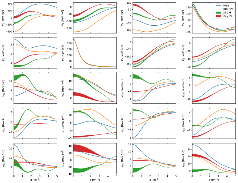
Figure 7: Momentum space local components of potentials as a function of the momentum transfer for several potentials: AV18 Wiringa:1994wb and the Granada DS-OPE Perez:2013mwa ; Perez:2013jpa , DS-$\chi$TPE Perez:2013oba ; Perez:2013cza and Gauss-OPE Perez:2014yla .

References

- (1) G. Audi, M. Wang, A.H. Wapstra, F.G. Kondev, M. MacCormick, X. Xu, Nucl. Data Sheets 120, 1 (2014)
- (2) S. Goriely, N. Chamel, J.M. Pearson, J. Phys. Conf. Ser. 665, 012038 (2016)
- (3) S. Aoki (HAL QCD), Prog.Part.Nucl.Phys. 66, 687 (2011).
- (4) S. Aoki, Eur. Phys. J. A49, 81 (2013).
- (5) S. Aoki, J. Balog, P. Weisz, Prog. Theor. Phys. 128, 1269 (2012).
- (6) S. Weinberg, Phys. Rev. 166, 1568 (1968).
- (7) S. Weinberg, Physica A96, 327 (1979).
- (8) J. Gasser, H. Leutwyler, Annals Phys. 158, 142 (1984).
- (9) G. Colangelo, J. Gasser, H. Leutwyler, Nucl. Phys. B603, 125 (2001).
- (10) J. Gasser, M.E. Sainio, A. Svarc, Nucl. Phys. B307, 779 (1988).
- (11) V. Bernard, N. Kaiser, J. Kambor, U.G. Meissner, Nucl. Phys. B388, 315 (1992).
- (12) T. Becher, H. Leutwyler, Eur. Phys. J. C9, 643 (1999).
- (13) S. Weinberg, Phys.Lett. B251, 288 (1990).
- (14) P.F. Bedaque, U. van Kolck, Ann. Rev. Nucl. Part. Sci. 52, 339 (2002).
- (15) E. Epelbaum, H.W. Hammer, U.G. Meissner, Rev. Mod. Phys. 81, 1773 (2009).
- (16) R. Machleidt, D. Entem, Phys.Rept. 503, 1 (2011).
- (17) H.W. Hammer, S. König, U. van Kolck (2019). 1906.12122
- (18) M. Pavon Valderrama, 1902.08172
- (19) R. Navarro Pérez, J.E. Amaro, E. Ruiz Arriola, J. Phys. G42, 034013 (2015).
- (20) R. Navarro Pérez, J.E. Amaro, E. Ruiz Arriola, J. Phys. G43, 114001 (2016).
- (21) R. Navarro Pérez, J.E. Amaro, E. Ruiz Arriola, 1202.6624
- (22) R. Navarro Pérez, J.E. Amaro, E. Ruiz Arriola, PoS QNP2012, 145 (2012).
- (23) B.D. Carlsson, A. Ekström, C. Forssén, D.F. Strömberg, G.R. Jansen, O. Lilja, M. Lindby, B.A. Mattsson, K.A. Wendt, Phys. Rev. X6, 011019 (2016).
- (24) W. Glöckle, The quantum mechanical few-body problem (Springer Berlin, 1983)
- (25) N. Hoshizaki, Prog. Theor. Phys. Suppl. 42, 107 (1969)
- (26) J. Bystricky, F. Lehar, P. Winternitz, J. Phys.(France) 39, 1 (1978)
- (27) P. LaFrance, P. Winternitz, Phys. Rev. D27, 112 (1983)
- (28) H. Kamada, W. Glöckle, H. Witała, J. Golak, R. Skibiński, Few-Body Systems 50, 231 (2011)
- (29) S. Okubo, R.E. Marshak, Annals of Physics 4, 166 (1958)
- (30) S. Mandelstam, Phys. Rev. 115, 1741 (1959)
- (31) R. Blankenbecler, M.L. Goldberger, N.N. Khuri, S.B. Treiman, Annals Phys. 10, 62 (1960)
- (32) J.M. Cornwall, M.A. Ruderman, Phys. Rev. 128, 1474 (1962)
- (33) R. Omnes, Phys. Rev. 137, B653 (1965)
- (34) J. Ruiz de Elvira, E. Ruiz Arriola, Eur. Phys. J. C78, 878 (2018).
- (35) M. Pavon Valderrama, E. Ruiz Arriola, Phys. Rev. C72, 044007 (2005)
- (36) J.C. Pupin, M.R. Robilotta, Phys. Rev. C60, 014003 (1999).
- (37) J.A. Oller, D.R. Entem, 1810.12242
- (38) M. Pavon Valderrama, E. Ruiz Arriola, Phys. Rev. C74, 054001 (2006).
- (39) M. Pavon Valderrama, E. Ruiz Arriola, Phys. Rev. C74, 064004 (2006), [Erratum: Phys. Rev.C75,059905(2007)],
- (40) E.E. Salpeter, H.A. Bethe, Phys. Rev. 84, 1232 (1951)
- (41) R. Blankenbecler, R. Sugar, Phys. Rev. 142, 1051 (1966)
- (42) F. Gross, Phys. Rev. 186, 1448 (1969)
- (43) V.G. Kadyshevsky, Nucl. Phys. B6, 125 (1968)
- (44) K. Chadan, P.C. Sabatier, Inverse problems in quantum scattering theory (Springer Science, 2012)
- (45) R.L. Workman, W.J. Briscoe, I.I. Strakovsky, Phys. Rev. C94, 065203 (2016).
- (46) H. Kohlhoff, H.V. von Geramb, Lect. Notes Phys. 427, 314 (1994)
- (47) A.A. Logunov, A.N. Tavkhelidze, Nuovo Cim. 29, 380 (1963)
- (48) A. Amghar, B. Desplanques, Nucl. Phys. A714, 502 (2003).
- (49) J. Nieves, E. Ruiz Arriola, Nucl. Phys. A679, 57 (2000).
- (50) R. Navarro Pérez, J.E. Amaro, E. Ruiz Arriola, Phys. Rev. C95, 064001 (2017).
- (51) E. Ruiz Arriola, J.E. Amaro, R. Navarro Pérez, Mod. Phys. Lett. A31, 1630027 (2016)
- (52) M. Piarulli et al, Phys. Rev. C94, 054007 (2016).
- (53) I.E. Lagaris, V.R. Pandharipande, Nucl. Phys. A359, 331 (1981)
- (54) V. Stoks, R. Klomp, C. Terheggen, J. de Swart, Phys.Rev. C49, 2950 (1994).
- (55) R.B. Wiringa, V. Stoks, R. Schiavilla, Phys.Rev. C51, 38 (1995).
- (56) R. Machleidt, Phys.Rev. C63, 024001 (2001).
- (57) F. Gross, A. Stadler, Phys.Rev. C78, 014005 (2008).
- (58) R. Navarro Pérez, J.E. Amaro, E. Ruiz Arriola, Phys. Rev. C88, 024002 (2013), [Erratum: Phys. Rev.C88,no.6,069902(2013)],
- (59) R. Navarro Pérez, J.E. Amaro, E. Ruiz Arriola, Phys. Rev. C88, 064002 (2013), [Erratum: Phys. Rev.C91,no.2,029901(2015)],
- (60) R. Navarro Pérez, J.E. Amaro, E. Ruiz Arriola, Phys. Rev. C89, 024004 (2014).
- (61) R. Navarro Pérez, J.E. Amaro, E. Ruiz Arriola, Few-Body Systems pp. 1–5 (2014).
- (62) R. Navarro Pérez, J.E. Amaro, E. Ruiz Arriola, Phys.Rev. C89, 064006 (2014).
- (63) S. Veerasamy, W.N. Polyzou, Phys. Rev. C84, 034003 (2011).
- (64) M. Pavon Valderrama, E. Ruiz Arriola, Phys. Rev. C80, 024001 (2009).
- (65) J. Aviles, Phys.Rev. C6, 1467 (1972)
- (66) D. Entem, E. Ruiz Arriola, M. Pavon Valderrama, R. Machleidt, Phys.Rev. C77, 044006 (2008).
- (67) R. Navarro Pérez, J.E. Amaro, E. Ruiz Arriola, Prog.Part.Nucl.Phys. 67, 359 (2012).
- (68) E. Ruiz Arriola, J. Ruiz de Elvira, 1906.10912
- (69) P. Fernandez-Soler, E. Ruiz Arriola, Phys. Rev. C96, 014004 (2017).
- (70) R. Navarro Pérez, J.E. Amaro, E. Ruiz Arriola, Phys. Lett. B724, 138 (2013).
- (71) V. Stoks, R. Kompl, M. Rentmeester, J. de Swart, Phys.Rev. C48, 792 (1993)
- (72) J. Dobaczewski, W. Nazarewicz, P.G. Reinhard, J. Phys. G41, 074001 (2014).
- (73) R. Navarro Pérez, E. Ruiz Arriola, J. Ruiz de Elvira, Phys. Rev. D91, 074014 (2015).
- (74) T. Ledwig, J. Nieves, A. Pich, E. Ruiz Arriola, J. Ruiz de Elvira, Phys. Rev. D90, 114020 (2014)
- (75) R. Navarro Pérez, J.E. Amaro, E. Ruiz Arriola, Int. J. Mod. Phys. E25, 1641009 (2016).
- (76) S. Wesolowski, N. Klco, R.J. Furnstahl, D.R. Phillips, A. Thapaliya, J. Phys. G43, 074001 (2016)
- (77) R. Navarro Pérez, J.E. Amaro, E. Ruiz Arriola, Phys. Rev. C91, 054002 (2015).
- (78) R. Navarro Pérez, J.E. Amaro, E. Ruiz Arriola, PoS CD12, 104 (2013).
- (79) I.R. Simo, J.E. Amaro, E. Ruiz Arriola, R. Navarro Pérez, J. Phys. G45, 035107 (2018).
- (80) D.B. Kaplan, M.J. Savage, Phys. Lett. B365, 244 (1996).
- (81) D.B. Kaplan, A.V. Manohar, Phys. Rev. C56, 76 (1997).
- (82) A. Calle Cordon, E. Ruiz Arriola, Phys. Rev. C78, 054002 (2008).
- (83) R. Navarro Pérez, J.E. Amaro, E. Ruiz Arriola, Few Body Syst. 54, 1487 (2013).
- (84) E. Ruiz Arriola, Symmetry 8, 42 (2016)
- (85) P. Reinert, H. Krebs, E. Epelbaum, Eur. Phys. J. A54, 86 (2018).
- (86) N. Kaiser, R. Brockmann, W. Weise, Nucl.Phys. A625, 758 (1997).
- (87) M.C.M. Rentmeester, R.G.E. Timmermans, J.L. Friar, J.J. de Swart, Phys. Rev. Lett. 82, 4992 (1999).
- (88) M.C.M. Rentmeester, R.G.E. Timmermans, J.J. de Swart, Phys. Rev. C67, 044001 (2003).
- (89) D.R. Entem, R. Machleidt, Y. Nosyk, Phys. Rev. C96, 024004 (2017).
- (90) A. Ekström, G. Baardsen, C. Forssén, G. Hagen, M. Hjorth-Jensen et al., Phys.Rev.Lett. 110, 192502 (2013).
- (91) N. Kaiser, Phys. Rev. C65, 017001 (2002).
- (92) A. Ekström, B.D. Carlsson, K.A. Wendt, C. Forssén, M. Hjorth-Jensen, R. Machleidt, S.M. Wild, J. Phys. G42, 034003 (2015)
- (93) V. Bernard, N. Kaiser, U.G. Meissner, Nucl. Phys. A615, 483 (1997).
- (94) A. Gezerlis, I. Tews, E. Epelbaum, M. Freunek, S. Gandolfi, K. Hebeler, A. Nogga, A. Schwenk, Phys. Rev. C90, 054323 (2014).
- (95) M. Piarulli, L. Girlanda, R. Schiavilla, R. Navarro Pérez, J.E. Amaro, E. Ruiz Arriola, Phys. Rev. C91, 024003 (2015).
- (96) N. Kaiser, S. Gerstendorfer, W. Weise, Nucl. Phys. A637, 395 (1998).
- (97) D.R. Entem, N. Kaiser, R. Machleidt, Y. Nosyk, Phys. Rev. C91, 014002 (2015).
- (98) J.E. Amaro, R. Navarro Pérez, E. Ruiz Arriola, Few Body Syst. 55, 977 (2014).
- (99) E. Ruiz Arriola, J.E. Amaro, R. Navarro Pérez, EPJ Web Conf. 137, 09006 (2017).
- (100) F. Calogero, Variable Phase Approach to Potential Scattering (Elsevier, 1967).