Swarm Engineering Through Quantitative Measurement of Swarm Robotic Principles in a 10,000 Robot Swarm

Abstract

When designing swarm-robotic systems, systematic comparison of algorithms from different domains is necessary to determine which is capable of scaling up to handle the target problem size and target operating conditions. We propose a set of quantitative metrics for scalability, flexibility, and emergence which are capable of addressing these needs during the system design process. We demonstrate the applicability of our proposed metrics as a design tool by solving a large object gathering problem in temporally varying operating conditions using iterative hypothesis evaluation. We provide experimental results obtained in simulation for swarms of over 10,000 robots.

1 Introduction

Swarm Robotics (SR) systems consist of large numbers of relatively few homogeneous groups of robots Şahin (2005). The main differentiating factors between SR systems and multi-agent robotics systems stem from the origins of SR as an offshoot of Swarm Intelligence (SI), which investigates algorithms and problem solving techniques inspired from natural systems such as bees, ants, and termites Labella and Dorigo (2006). The main properties are:

Scalability. SR systems have no centralized control/single point of failure, which makes them scalable to hundreds or thousands of agents, much like their natural counterparts Lerman et al. (2004).

Emergence. Agents in SR systems collectively find solutions to a problem at hand that they cannot solve alone Cotsaftis (2009). More precisely, emergent behaviors arising through this collective search process refer to the appearance of self-organization within the system due to robot interactions Winfield and Sa (2005); Galstyan et al. (2005). Such behaviors cannot be predicted from individual agent behaviors (i.e., it is the set difference between micro and macro swarm behavior Szabo et al. (2014)).

Flexibility. In SR systems all decisions are made by individual agents based on locally available information from neighbors as well as their own limited sensor data. This results in reactive and adaptive swarm-level behaviors that attempt to mitigate adversity and exploit beneficial changes in dynamic environmental conditions and/or problem definitions Harwell and Gini (2018); Winfield et al. (2008).

Robustness. The number of agents in a SR system is unlikely to remain constant during execution, and can fluctuate due to introduction of new agents and robotic failures. A high failure rate within a swarm may slow its operation, but it does not prevent the accomplishment of its objective Lerman et al. (2004), in contrast to many multi-agent systems which cannot withstand such losses.

The duality between SR and natural systems enables effective parallels to be drawn with many naturally occurring problems, such as foraging, collective transport of heavy objects, environmental monitoring/cleanup, self-assembly, exploration, and collective decision making Şahin (2005); Hecker and Moses (2015). As a result, SR systems are especially well suited to tackle complex tasks in environments where robustness and flexibility of robotic systems is key to success, such as space Rouff and others (2004). Other real-world problems with applicable SR solutions include tracking lake health, clearing a corridor on a mining operation, hazardous material cleanup, and search and rescue Şahin (2005); Hecker and Moses (2015); Labella and Dorigo (2006).

In a foraging task, robots gather objects from across a finite operating arena and bring them to a central location under various conditions and constraints. Foraging is one of the most extensively studied applications of SR, due to its straightforward mapping to real-world applications Hecker and Moses (2015). In this paper, we study scalability, emergence, and flexibility in the context of a foraging task.

We present measurement methods of swarm scalability and emergent self-organization using projected vs. observed performance increases and expected vs. actual performance losses, respectively, as swarm sizes increase. We show that they provide valuable input into iterative SR system design and algorithm selection for a particular problem/swarm size. We also present a methodology to measure swarm flexibility (its ability to react and adapt to changing environmental conditions) using mathematical methods of curve similarity. By correlating temporal curves of swarm performance with curves of varying environmental conditions, we can quantify how much performance should be expected to be gained or lost between scenarios with different operating conditions or task parameters. We show that our methodology enables mathematically grounded algorithm selection decisions through quantitative comparisons of similarity between the target operating conditions and those in which the algorithm was developed and tested.

We evaluate our proposed metrics using a simulated design process to demonstrate the correctness of predictive hypotheses framed using our measures as swarm sizes are scaled up to 16,384 robots. Results indicate that explicit quantification of different facets of a swarm’s intelligence across all tested scales is possible using our proposed measures. This quantification is shown to provide insight into what properties the “best” method for solving the problem at hand should have by exposing predictive differences in swarm response to external and internal stimuli not evident from raw performance curves.

1.1 Background and Related Work

In recent years, many theoretical SR system design tools have become available Matthey et al. (2009); Correll (2008); Lopes et al. (2016); Hamann (2013). These tools have made it easier to conduct mathematical analysis of algorithms and derive analytical, rather than weakly inductive proofs of correctness Winfield et al. (2008). Despite this, there has not been a corresponding increase in the average swarm sizes used to evaluate new algorithms (Notable exceptions include Lopes et al. (2016) (600 robots), Hecker and Moses (2015) (768 robots), Hamann and Wörn (2008) (375 robots)). Investigation of simple behaviors such as pattern formation, localization, or collective motion, where design and computational complexity do not inherently limit scalability, is generally evaluated with relatively small scales (~40 robots Winfield et al. (2008)). Methods for more complex behaviors, such as foraging Ferrante et al. (2015); Pini et al. (2011a) (20 robots), Pini et al. (2011b) (30 robots), task allocation Correll (2008) (25 robots) are likewise tested at similar scales.

We believe that the lack of evaluation of large SR systems is partially due to a lack of standardized comparison methods to accurately characterize swarm performance across problem scales and domains. Building on previous works Harwell and Gini (2018); Hecker and Moses (2015), we propose a swarm scalability measure analogous to projected vs. observed speedup when core count is increased on supercomputing clusters.

Within SR, no widely accepted theory of self-organizing systems exists Hamann and Wörn (2008); Galstyan et al. (2005). Cotsaftis Cotsaftis (2009) presents a control-theoretic model of emergence, distinguishing between complicated systems which can be studied by the methods of scientific reductionism, and complex systems which originate from the existence of a threshold above which interaction between system components overtakes outside interactions, leading to system self-organization and new behavior not predictable from component study, similar to Georgé and Gleizes (2005). While many papers cite evidence that their algorithms exhibit emergent behavior Liu et al. (2007); Frison et al. (2010); Harwell and Gini (2018); Matthey et al. (2009), or even prove simple emergent properties via temporal logic (Winfield and Sa (2005)), few provide a quantitative method for measuring emergence (with the exception of Szabo et al. (2014), who used robot nearest-neighbor calculations to calculate a degree of interaction for the swarm). We present an empirical method for measuring the level of self organization present in a swarm by measuring the linearity of inter-robot interference as the swarm size is increased, as a small step towards the development of a more general emergence theory.

While it is common to evaluate swarms under conditions different than their development, the resultant claims of flexibility due to performance similarity across scenarios is strictly qualitative, due to a lack of mathematical quantification of “difference” in scenario conditions as a factor in performance comparisons. We utilize curve similarity methods from Jekel et al. Jekel et al. (2018), who tested different mathematical curve similarity measures in various noise and normalization conditions to provide the required mathematical basis. We derive a difference measure between expected and observed performance in temporally variable environmental conditions, and use it to quantify the swarm reactivity (how closely swarm performance tracks changing environmental conditions in time) and adaptability (how well the swarm exploits or resists beneficial or adverse changes in environmental conditions).

2 Proposed Quantitative Measurements

2.1 Swarm Scalability

Hecker and Moses Hecker and Moses (2015) calculated scalability $S(N)=P(N)/N$ as per-robot efficiency using a performance measure $P(N)$, where $N$ is the size of the swarm. $P(N)$ is general in nature, and can measure time to complete a certain number of tasks, task completion rate, etc. While this measure provides some insight into scalability, it is not predictive (e.g. given $P(N)$, we cannot plausibly estimate $P({2}{N})$ without retroactively charting $S(N)$ across a range of $N$).

We extend $P(N)$ to $P(N,\kappa,t)$, where $\kappa$ is the swarm control algorithm plus algorithmic parameters and $t$ is the current discrete timestep (swarm performance varies temporally, tracing out a performance curve). For a simulation of length $T$ broken into $t$ timesteps, our generalized formulation allows us to simultaneously analyze (1) cumulative performance by summing across all $t\in{T}$, (2) temporally varying performance curves via pairwise point comparison for each $t\in{T}$ (see Section 2.3).

We define a more predictive scalability metric for use as an iterative system design tool using the Karp-Flatt metric Karp and Flatt (1990). Traditionally, the serial fraction $\mathbf{e}$ of the Karp-Flatt metric measures the level of parallelization of a particular program, with smaller values indicating high parallelization and plausibly expected speedups if more computational resources are added. In SR, it measures the intelligence of a swarm by exposing the part of $P(N,\kappa,T)$ that did not utilize inter-robot cooperation.

Scalability: $\mathbf{e}(N_{1},N_{2},\kappa)$ for two swarms of sizes $N_{1}$ and $N_{2}$ ($N_{2}>N_{1}$) controlled by a method $\kappa$ is defined as:

$$\mathbf{e}(N_{1},N_{2},\kappa)=\frac{\frac{1}{\phi(N_{1},N_{2},\kappa)}-\frac{1}{N_{1}}}{1-\frac{1}{N_{1}}}$$ (1)

where

$$\phi(N_{1},N_{2},\kappa)=\sum_{t\in{T}}\frac{P(N_{2},\kappa,t)}{\frac{N_{2}}{N_{1}}~{}P(N_{1},\kappa,t)}$$ (2)

is based on a swarm’s projected vs. observed performance. Intuitively, Eqn. (2) can be understood in terms of computational workloads: if a job takes $T$ seconds with $N$ resources, ideally it will take $T/2$ seconds with $2N$ resources in a perfectly parallelizable system.

2.2 Swarm Emergence via Self-Organization

We can infer from Cotsaftis Cotsaftis (2009) that SR systems with a high degree of local interactivity should exhibit higher levels of self-organization (and therefore emergent behavior, as established by Georgé and Gleizes (2005)) than systems with a low degree of interactivity Szabo et al. (2014); Galstyan et al. (2005); Winfield and Sa (2005). We can therefore approximately measure a swarm’s emergent behavior by measuring its self organization.

We calculate (post-hoc) the expected number of robots engaged in collision avoidance (as opposed to doing useful work) in a swarm of size $N$, and use this to derive the amount of time lost due to inter-robot interference on each timestep $t$, denoted as $t_{lost}^{N}(t)$. This can then be used to compute the per-timestep fraction of overall performance loss ($P_{lost}(N,\kappa,t)$) due to inter-robot interference as follows:

$$P_{lost}(N,\kappa,t)=\begin{cases}{P(1,\kappa,t)}{t_{lost}^{1}(t)}&\text{if N = 1}\\ P(N,\kappa,t){t_{lost}^{N}(t)}\\ ~{}-{N}{P_{lost}(1,\kappa,t)}&\text{if N $>$ 1}\\ \end{cases}$$ (3)

For $N\geq 1$ we subtracted the interference that would have occurred in a non-interactive swarm of $N$ robots (i.e. a swarm of size $N$ which only interacted with arena boundaries). Let $M=\{1,2,4,\ldots{},m_{max}$} be a logarithmically distributed (powers of two) set. If we then compute Eqn. (3) for each $m\in{M}$, sub-linear fractional losses between $P_{lost}(m_{i-1},\kappa,t)$ and $P_{lost}(m_{i},\kappa,pt)$ indicate that the method $\kappa$ is scalable in the neighborhood of sizes near $m_{i}$ (i.e., doubling the swarm size does not double the amount of inter-robot interference).

Using Eqn. (3), we quantify a swarm’s ability to detect and eliminate non-cooperative situations between agents Georgé and Gleizes (2005) (e.g., frequent inter-robot interference) as swarm size is increased. Our self-organization measure can therefore be used to measure the “intelligence” of different algorithms deployed in a swarm in terms of their to manage space without sacrificing performance.

Self-organization: $Z(m_{i},\kappa)$ is defined as:

$$Z(m_{i},\kappa)=\sum_{t\in{T}}1-\frac{1}{1+e^{-\theta_{Z}(m_{i},\kappa,t)}}$$ (4)

where

$$\theta_{Z}(m_{i},\kappa,t)=P_{lost}(m_{i},\kappa,t)-\frac{m_{i}}{m_{i-1}}{P_{lost}(m_{i-1},\kappa,t)}$$ (5)

Intuitively, Eqn. (5) indicates that if the proportional increases in fractional performance losses observed at swarm sizes $m_{i-1}$ and $m_{i}$ are sublinear ($\theta_{Z}(m_{i},\kappa,t)\leq 0$), then Eqn. (4) $\rightarrow 1.0$, indicating that self-organization occurred, and vice versa with Eqn. (4) $\rightarrow 0.0$ for superlinear increases. We note that this definition of self-organization assumes that a swarm is operating in a bounded space; this is not generally a limiting assumption, as such restrictions are common in real-world applications such as warehouses Pini et al. (2011b).

2.3 Swarm Flexibility via Reactivity and Adaptability

We define a swarm’s flexibility in terms of its ability to adapt to changes in the external environment over time, which can include (1) costs of performing a particular action (e.g., picking up/dropping an object in the case of foraging), (2) maximum robot speed, modeling changing environmental conditions (e.g., wheeled robots buffeted in variable winds) or the performance of some tasks more slowly than others (e.g., carrying objects of different sizes during foraging).

Let $I_{ec}(t)$ and $V_{dev}(t)$ be continuous, one-dimensional signals representing respectively (1) the ideal environmental conditions that a given swarm was developed in, (2) the waveform of a deviation from $I_{ec}(t)$. We have restricted our study to one-dimensional characterizations of environmental conditions, but extensions to higher dimensions should be relatively straightforward.

Intuitively, we define swarm reactivity $R(N,\kappa)$ as how closely the observed performance curve $P(N,\kappa,t)$ tracks an applied variance $V_{dev}(t)$. In a swarm with optimal reactivity $R^{*}(N,\kappa)$, $P(N,\kappa,t)=c_{t}{V_{dev}(t)}$, where $c_{t}$ is a non-negative per-timestep constant (i.e., instantaneous tracking).

Reactivity $R(N,\kappa)$ is defined as:

$$R(N,\kappa)=DTW(P_{R^{*}}(N,\kappa,t),P(N,\kappa,t))$$ (6)

where we define $DTW(X,Y)$ to be a Dynamic Time Warp similarity measure between two discrete curves $X$ and $Y$, based upon the conclusions in Jekel et al. (2018). We note that (1) DTW correctly matches temporally shifted sequences of applied variance and observed performance (achieving $R^{*}(N,\kappa)$ is not possible for realistic swarms), (2) DTW exhibits robustness to signal noise, and SR systems are inherently stochastic.

Formally, we derive $R(N,\kappa)$ for a stepped experiment of length $T$ using $Q:[X,a,b]\rightarrow X^{\prime}$, with $a,b\in\mathbb{N}$, as a mapped min-max normalization of a curve $X$ into the range $[a,b]$:

$$X^{\prime}=\frac{(b-a)(X-\min{X})}{\max{X}-\min{X}}+a$$ (7)

We construct the optimal performance curve $P_{R^{*}}(N,\kappa,t)$ of a maximally reactive method $\kappa$ by normalizing the difference curve of $V_{dev}(t)-I_{ec}(t)$ to the scale of the observed performance under ideal conditions:

$$P_{R^{*}}(N,\kappa,t)=Q( V_{dev}(t),$$ (8)

$$\min(P_{ideal}(N,\kappa,t)),$$

$$\max(P_{ideal}(N,\kappa,t)))$$

Finally, the adaptability $A(N,\kappa)$ of a swarm can be thought of as its ability to (1) minimize performance losses under adverse conditions ($V_{ec}(t)\geq I_{ec}(t)$), (2) proportionally exploit beneficial deviations from ideal conditions ($V_{ec}(t)<I_{ec}(t)$).

Adaptability: $A(N,\kappa)$ is defined as the $DTW(X,Y)$ similarity to the optimal adaptability curve $P_{A^{*}}(N,\kappa,t)$:

$$A(N,\kappa)=DTW(P_{A^{*}}(N,\kappa,t),P(N,\kappa,t))$$ (9)

Formally, we define $P_{A^{*}}(N,\kappa)$ as:

$$P_{A^{*}}(N,\kappa,t)=\begin{cases}\frac{{c_{t}}V_{ec}(t)}{I_{ec}(t)}R(N,\kappa)&\text{if $V_{ec}(t)<I_{ec}(t)$}\\ P_{ideal}(N,\kappa,t)&\text{else}\end{cases}$$ (10)

where $c_{t}$ is a positive per-timestep constant.

We briefly note that a weighted combination of Eqn. (6) and Eqn. (9) could be employed as a design tool to gain insight into the most suitable method for a set of target operating conditions, and reduce the simulation-reality gap Hecker and Moses (2015); Brutschy and others (2015).

3 Example of Application to a Foraging Task

We evaluate our proposed methodology by simulating the iterative SR design process for a large-scale foraging application that (1) has 10,000 robots available for use (not all robots need to be utilized) (2) has an operating area $\geq 4,000m^{2}$, (3) has temporally variable operating conditions which can suddenly change from favorable to unfavorable (or vice versa) at some point during system operation (i.e., a passing storm in an outdoor environment).

We utilize our derived metrics to iteratively form and test hypotheses as we scale swarm and arena size to the parameters of our target application in order to refine our estimate of which method $\kappa$ provides maximum performance.

We use homogeneous swarms and the following candidates controllers $\kappa\in${CRW,DPO,GP-DPO} from Harwell and Gini (2018), summarized briefly here. In Correlated Random Walk (CRW) swarms, robots perform a correlated random walk until they acquire an object, which they then transport to the nest using phototaxis (i.e., motion in response to light). In Decaying Pheromone Object (DPO) swarms, robots track seen objects using exponentially decaying pheromones, and determine the “best” object to acquire using derived information relevance. In Greedy Partitioning DPO (GP-DPO) swarms, robots stochastically choose to do either (1) the entire foraging task themselves (i.e., retrieving an object and bringing it to the nest), or (2) one of two subtasks of bringing an acquired object to an intermediate drop site (cache), or picking one up from a cache and bringing it to the nest.

The experiments described in this paper have been carried out in the ARGoS Pinciroli et al. (2012) simulator. We employ a dynamical physics model of the robots in a three dimensional space for maximum fidelity (robots are still restricted to motion in the XY plane), using a model of the s-bot developed by Dorigo (2005). We use a single-source foraging experiment design Harwell and Gini (2018); Ferrante et al. (2015); Pini et al. (2011a), in which all objects are concentrated at the far end of a rectangular, obstacle-free arena, shown in Fig.1. For all experiments we average the results of 50 experimental runs of $T=10,000$ seconds for each $\kappa\in$ {CRW,DPO,GP-DPO}.

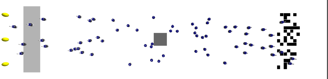
Figure 1: A screen shot of a simulation with multiple robots, objects to be collected, and the nest on the left side.

3.1 Ideal Conditions

We begin with a $32\times 16=368~{}m^{2}$ arena, and define $P(N,\kappa,T)$ for ideal operating conditions as the cumulative number of objects gathered within a simulation up to time $t=T$. We first evaluate our scalability measure on small swarms of up to 1,024 robots in this arena (Fig. 2).

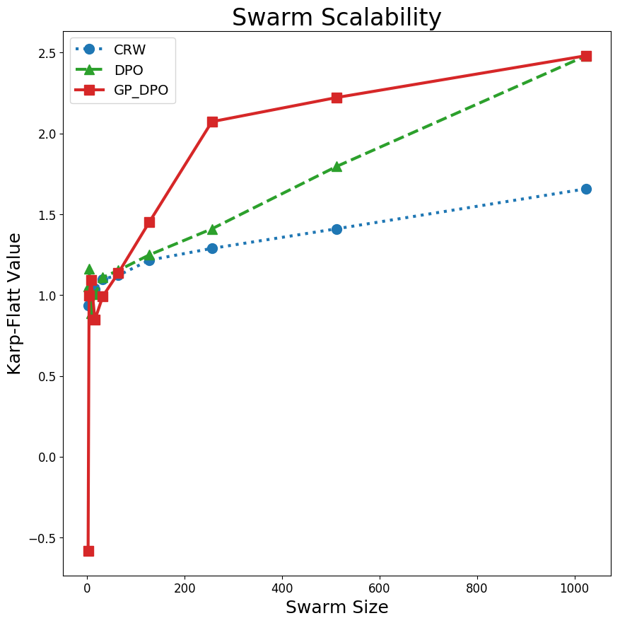
Figure 2: Swarm scalability $\mathbf{e}(N_{1},N_{2},\kappa)$ for the 32$\times$16 scenario. CRW swarms are the most parallelizable (i.e., proportional performance increases are likely at higher values of $N$).

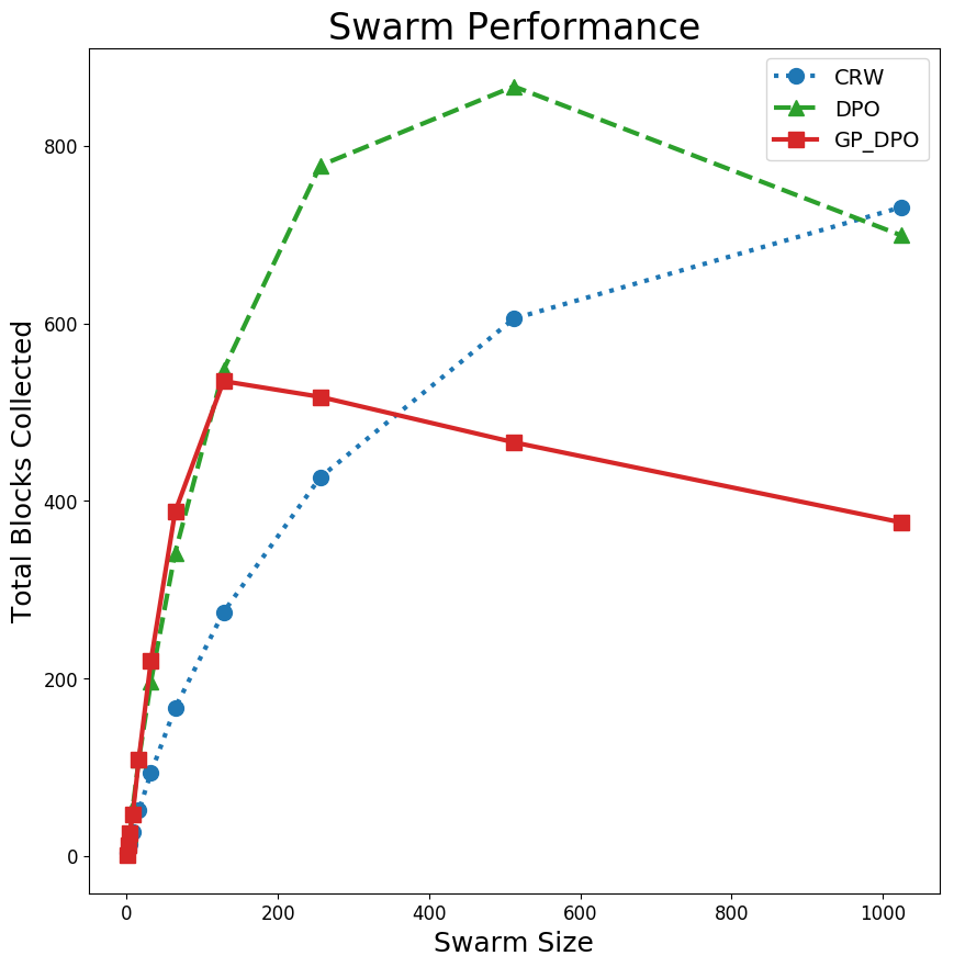
Figure 3: Swarm performance $P(N,\kappa)$ for the $32\times 16$ scenario.

The results in Fig. 2 confirm our intuition that as swarm sizes begin to approach natural scales in confined, obstacle-free spaces, randomized motion is the most scalable navigation method. However, looking at the performance curves for the $32\times 16$ scenario in Fig. 3, we see that for smaller swarm sizes, the more “intelligent” DPO/GP-DPO approaches perform better. The trendlines for scalability in Fig. 2 and performance in Fig. 3 for DPO and GP-DPO swarms are consistent: the asymptotic behavior of the exponential performance curves (the characteristic s-shape of swarms) are ordered according to trends of the scalability curves, demonstrating the predictive insight possible with our metric.

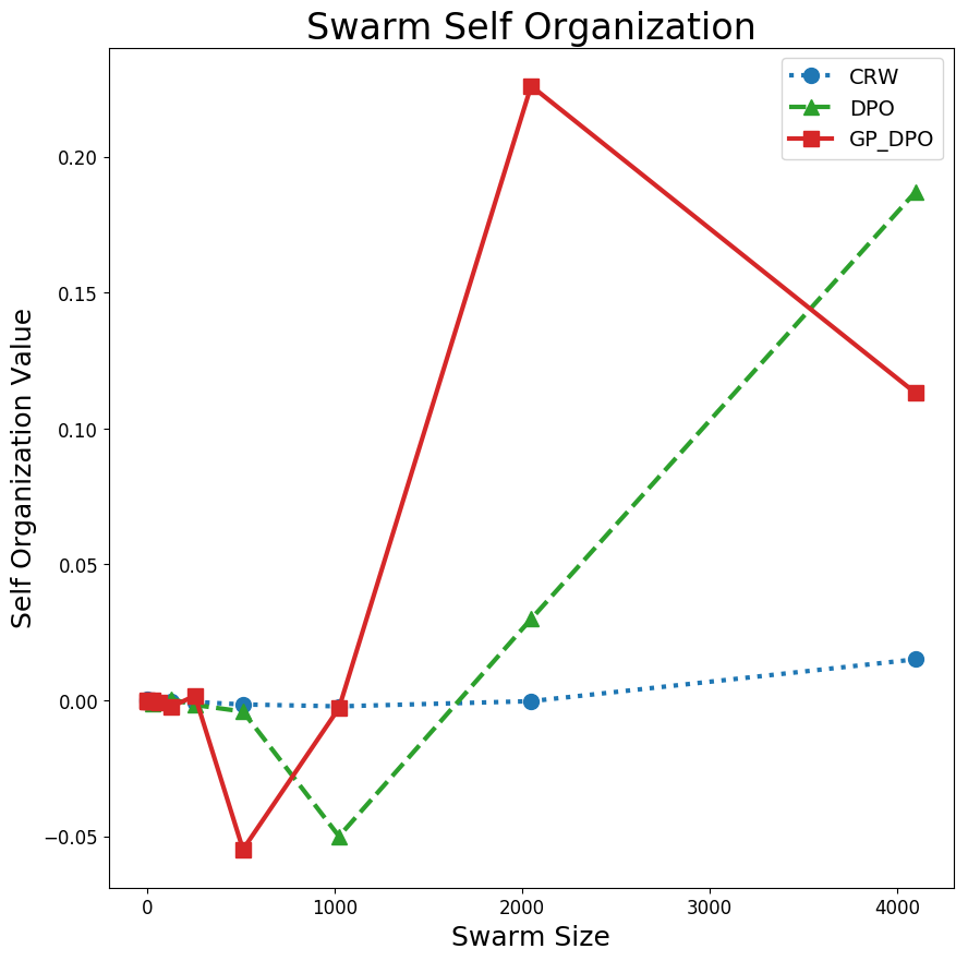
Figure 4: Swarm self-organization $Z(N,\kappa)$ for the $64\times 32$ scenario. Asymptotic trendlines suggest the hypothesis that DPO swarms have the greatest potential for self-organization with $N>4,096$.

Scaling up swarm/problem size to 4,096 robots and $64\times 32=1,388~{}m^{2}$ arena respectively, we evaluate our self-organization metric (Fig. 4). Correlating the self-organization and performance curves in Fig. 4 and Fig. 5, respectively, we see that for DPO and GP-DPO swarms the sizes at which maximum $P(N,\kappa,T)$ and first negative $Z(N,\kappa)$ occur are approximately identical, demonstrating the usefulness of our self-organization metric as a predictive design tool (i.e. no need to continue to scale up a method once you observe a negative $Z(N,\kappa)$ value). Finally, in CRW swarms we observe that the consistently low levels of self-organization nevertheless correlate with performance trendlines suggesting the highest possible performance of the three tested methods at large sizes. In mathematical terms, we gain the insight that the second derivative of the self-organization curves is just as important as the first derivative (which gives the asymptotic trendline of the self-organization for a given $\kappa$) in predicting asymptotic performance. We hypothesize that this is due to a threshold problem/swarm size above which the more “intelligent” DPO/GP-DPO methods break down due to high levels of inter-robot interference, while the more simplistic CRW method is able to more efficiently scale beyond it.

Building on these insights, we hypothesize CRW swarms will have the highest level of performance as we scale swarm/problem size to 16,384 robots and a $96\times 48=4,608~{}m^{2}$ arena respectively, which is confirmed by Fig. 6.

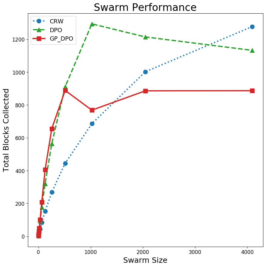
Figure 5: Swarm performance $P(N,\kappa)$ for the $64\times 32$ scenario.

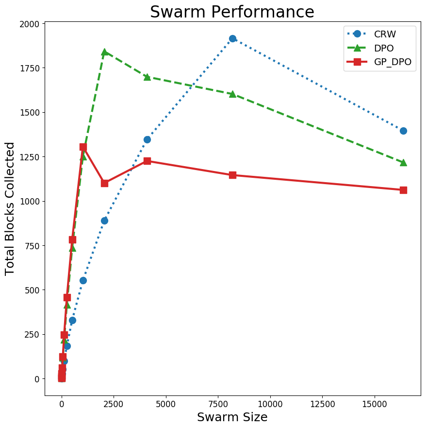
Figure 6: Swarm performance $P(N,\kappa)$ across all $m\in M$ for the 96$\times$48 scenario.

3.2 Temporally Varying Conditions

We next evaluate our three candidate approaches with temporally varying operating conditions. We apply throttling functions to the maximum robot speed while carrying a block using the Heaviside $H(t)$ step functions with amplitude $\beta=\{0.1,0.2,0.4,0.8\}$, and set $\alpha=\frac{T}{2}$:

$$V_{1}(t,\alpha)={\beta}\times{H}(t-\alpha)=\begin{cases}0&\text{if $t-\alpha<0$}\\ \frac{\beta}{2}&\text{if $t-\alpha=0$}\\ A&\text{if $t-\alpha>0$}\\ \end{cases}$$ (11)

$$V_{2}(t,\alpha)=\beta-V_{1}(t,\alpha)$$ (12)

Eqn. (11) models a sudden increase in the adversity of the swarm’s operating environment, and Eqn. (12) models a sudden decrease in the adversity of the swarm’s operating environment. We hypothesize that GP-DPO swarms will be the most reactive and adaptive of all tested $\kappa$, due to (1) the relatively high values of $Z(m_{i},\kappa)$ previously observed (even though they are inconsistent across swarm sizes), and (2) their ability to collectively choose a task less impacted by the applied variance (i.e., utilizing the central cache).

We see in Fig. 7 and Fig. 8 that all swarms show increasing levels of reactivity/adaptability with increasing $\beta$ in $V_{2}(t,\alpha)$, indicating that all $\kappa$ have the ability to proportionally react and adapt to changing environmental conditions. The plots in Fig. 7 and Fig. 8 confirm our hypothesis that the GP-DPO swarms would be the most reactive/adaptive, and demonstrate for the first time a mathematical framework for equitable comparison of methods across different scenarios. CRW swarms, while not nearly as reactive, are also very adaptive, which intuitively makes sense for a biomimetic method.

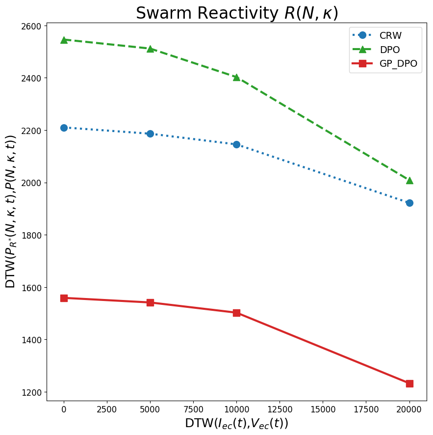
Figure 7: Swarm reactivity $R(N,\kappa)$ with $V_{2}(t,\alpha)$. Lower Y-values indicate less distance to $P_{R^{*}}(N,\kappa,t)$ and therefore greater reactivity.

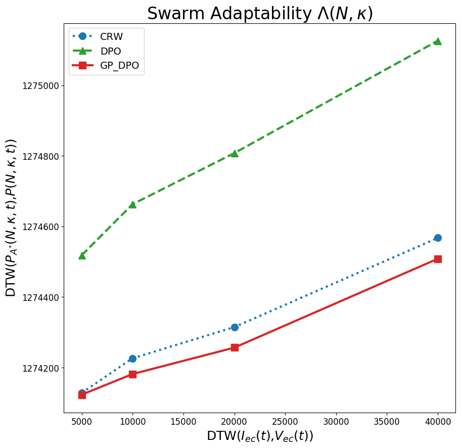
Figure 8: Swarm adaptability $A(N,\kappa)$ with an applied variance of $V_{2}(t,\alpha)$. Lower Y-values indicate less distance to $P_{A^{*}}(N,\kappa,t)$ and hence greater adaptability.

4 Discussion

From the progression in Section 3, we have been able to use the insights gained through our proposed measures at each stage of our simulated design process to build accurate hypotheses about what is likely to occur as we continue to scale up to meet the demands of our example application. The DPO method provides almost the same performance with 2,048 robots as the CRW method does with 8,192, but it is the least reactive and the least adaptive of the chosen methods. Both of these are important factors in determining method suitability in our target application, and we therefore select the CRW method with $\sim$8,192 robots to meet our needs. We did not perform method recommendations for any of the smaller arena and swarm sizes, though it is clear from the progression above that our proposed metrics can effectively be used to select the most appropriate method at any scale. While not rigorous, Section 3 provides a weakly inductive proof of the correctness and utility of the proposed metrics within the foraging domain, if not more broadly.

4.1 Conclusions and Future Work

We have presented three measurement methods for more precise characterization of swarm scalability, emergence, and flexibility, in order to provide mathematical tools to aid in the iterative design process of SR systems. We validated our proposed measures in the context of a foraging task, and have shown that they provide intuitive insight into recommending a given method for a given problem size and operating conditions. A next step in this work would be to develop a method for quantitative measurement of robustness (e.g., temporally varying swarm sizes and sensor/actuator noise). In order to facilitate future research and collaboration, the code used for this research is open source, and can be found at https://github.com/swarm-robotics/fordyca.

References

- Brutschy and others (2015) Arne Brutschy et al. The TAM: abstracting complex tasks in swarm robotics research. Swarm Intelligence, 9(1):1–22, 2015.
- Correll (2008) Nikolaus Correll. Parameter estimation and optimal control of swarm-robotic systems: A case study in distributed task allocation. In Proc. IEEE Int’l Conf. on Robotics and Automation, pages 3302–3307, May 2008.
- Cotsaftis (2009) Michel Cotsaftis. An emergence principle for complex systems. In Complex Sciences, pages 1105–1117. Springer Berlin Heidelberg, 2009.
- Dorigo (2005) Marco Dorigo. Swarm-bot: An experiment in swarm robotics. In Proc. IEEE Swarm Intelligence Symposium, pages 199–207, 2005.
- Ferrante et al. (2015) Eliseo Ferrante, Ali Emre Turgut, Edgar Duéñez-Guzmán, Marco Dorigo, and Tom Wenseleers. Evolution of Self-Organized Task Specialization in Robot Swarms. PLoS Computational Biology, 11(8), 2015.
- Frison et al. (2010) Marco Frison, Nam Luc Tran, Nadir Baiboun, Arne Brutschy, Giovanni Pini, Andrea Roli, Marco Dorigo, and Mauro Birattari. Self-organized task partitioning in a swarm of robots. In Swarm Intelligence, LNCS 6234, pages 287–298. Springer, 2010.
- Galstyan et al. (2005) Aram Galstyan, Tad Hogg, and Kristina Lerman. Modeling and mathematical analysis of swarms of microscopic robots. In Proc. IEEE Swarm Intelligence Symposium, SIS 2005, pages 209–216, 2005.
- Georgé and Gleizes (2005) Jean-Pierre Georgé and Marie-Pierre Gleizes. Experiments in Emergent Programming Using Self-organizing Multi-agent Systems. Multi-Agent Systems and Applications IV, 3690:450–459, 2005.
- Hamann and Wörn (2008) Heiko Hamann and Heinz Wörn. A framework of space-time continuous models for algorithm design in swarm robotics. Swarm Intelligence, 2(2-4):209–239, 2008.
- Hamann (2013) Heiko Hamann. Towards swarm calculus: urn models of collective decisions and universal properties of swarm performance. Swarm Intelligence, 7:145–172, 2013.
- Harwell and Gini (2018) John Harwell and Maria Gini. Broadening applicability of swarm-robotic foraging through constraint relaxation. IEEE Int’l Conf. on Simulation, Modeling, and Programming for Autonomous Robots (SIMPAR), pages 116–122, May 2018.
- Hecker and Moses (2015) Joshua P. Hecker and Melanie E. Moses. Beyond pheromones: evolving error-tolerant, flexible, and scalable ant-inspired robot swarms. Swarm Intelligence, 9(1):43–70, 2015.
- Jekel et al. (2018) Charles F. Jekel, Gerhard Venter, Martin P. Venter, Nielen Stander, and Raphael T. Haftka. Similarity measures for identifying material parameters from hysteresis loops using inverse analysis. International Journal of Material Forming, pages 1–24, 2018.
- Karp and Flatt (1990) Alan H. Karp and Horace P. Flatt. Measuring parallel processor performance. Commun. ACM, 33(5):539–543, May 1990.
- Labella and Dorigo (2006) Thomas H. Labella and Marco Dorigo. Division of labor in a group of robots inspired by ants’ foraging behavior. ACM Trans. on Autonomous and Adaptive Systems (TAAS), 1(1):4–25, September 2006.
- Lerman et al. (2004) Kristina Lerman, Alcherio Martinoli, and Aram Galstyan. A review of probabilistic macroscopic models for swarm robotic systems. In Swarm Robotics, LNCS 3342. Springer Berlin Heidelberg, 2004.
- Liu et al. (2007) W. Liu, a. F. T. Winfield, J. Sa, J. Chen, and L. Dou. Towards energy optimization: Emergent task allocation in a swarm of foraging robots. Adaptive Behavior, 15(3):289–305, 2007.
- Lopes et al. (2016) Yuri K. Lopes, Stefan M. Trenkwalder, André B. Leal, Tony J. Dodd, and Roderich Groß. Supervisory control theory applied to swarm robotics. Swarm Intelligence, 10(1):65–97, 2016.
- Matthey et al. (2009) Löic Matthey, Spring Berman, and Vijay Kumar. Stochastic strategies for a swarm robotic assembly system. Proc. IEEE Int’l Conf. on Robotics and Automation, pages 1953–1958, 2009.
- Pinciroli et al. (2012) Carlo Pinciroli et al. ARGoS: a modular, parallel, multi-engine simulator for multi-robot systems. Swarm Intelligence, 6(4):271–295, 2012.
- Pini et al. (2011a) Giovanni Pini, Arne Brutschy, Mauro Birattari, and Marco Dorigo. Task partitioning in swarms of robots: Reducing performance losses due to interference at shared resources. In Informatics in Control Automation and Robotics, LNEE 85, pages 217–228. Springer, 2011.
- Pini et al. (2011b) Giovanni Pini, Arne Brutschy, Marco Frison, Andrea Roli, Marco Dorigo, and Mauro Birattari. Task partitioning in swarms of robots: An adaptive method for strategy selection. Swarm Intelligence, 5(3-4):283–304, 2011.
- Rouff and others (2004) Christopher Rouff et al. Properties of a formal method for prediction of emergent behaviors in swarm-based systems. In Proc. 2nd International Conference on Software Engineering and Formal Methods, 2004.
- Şahin (2005) Erol Şahin. Swarm robotics: From sources of inspiration to domains of application. In Swarm Robotics, LNCS 3342, pages 10–20. Springer, 2005.
- Szabo et al. (2014) Claudia Szabo, Yong Meng Teo, and Gautam K. Chengleput. Understanding complex systems: Using interaction as a measure of emergence. In Proc. Winter Simulation Conference, pages 207–218, Dec 2014.
- Winfield and Sa (2005) Alan F. T. Winfield and Jin Sa. On formal specification of emergent behaviours in swarm robotic systems. Science, pages 363–371, 2005.
- Winfield et al. (2008) Alan F. T. Winfield, Wenguo Liu, Julien Nembrini, and Alcherio Martinoli. Modelling a wireless connected swarm of mobile robots. Swarm Intelligence, 2(2-4):241–266, December 2008.