Zero-one laws for existential first order sentences of bounded quantifier depth

Abstract.

For any fixed positive integer $k$, let $\alpha_{k}$ denote the smallest $\alpha\in(0,1)$ such that the random graph sequence $\left\{G\left(n,n^{-\alpha}\right)\right\}_{n}$ does not satisfy the zero-one law for the set $\mathcal{E}_{k}$ of all existential first order sentences that are of quantifier depth at most $k$. This paper finds upper and lower bounds on $\alpha_{k}$, showing that as $k\rightarrow\infty$, we have $\alpha_{k}=\left(k-2-t(k)\right)^{-1}$ for some function $t(k)=\Theta(k^{-2})$. We also establish the precise value of $\alpha_{k}$ when $k=4$.

1. Introduction

Given a graph $G$, we denote by $V(G)$ the set of its vertices and by $E(G)$ the set of its edges; when $G$ is clear from the context, we simply write $V$ and $E$ respectively. We set $e(G)=|E(G)|$ and $v(G)=|V(G)|$. For two vertices $x$ and $y$ in $V$, we say that $\{x,y\}\in E$ when $x$ and $y$ is adjacent. When the graph and its edge set are evident, we also alternatively use the notation $x\sim y$. We denote by $\mathbb{N}$ the set of all positive integers and by $\mathbb{N}_{0}$ the set of all non-negative integers.

A sentence is a formula in mathematical logic that does not have free variables (see [[11], Subsection 2.1] for basic definitions in mathematical logic). The first order logic on graphs comprises finite sentences involving the following components:

• the vertices as propositional variables, denoted in general by lower case letters such as $x,y,z\ldots$;

• the relation of vertex equality (denoted $x=y$) and the relation of vertex adjacency (denoted $x\sim y$);

• Boolean connectives $\wedge,\vee,\neg,\implies,\Leftrightarrow$;

• existential (denoted $\exists$) and universal (denoted $\forall$) quantification, allowed only over vertices.

We refer the reader to [11, 12, 13, 5] for further reading on first order logic. Examples of first order sentences include

$$\exists x[\forall y[\neg x\sim y]],$$

which expresses the property of a graph that it contains an isolated vertex, and

$$\exists x[\exists y[[x\sim y]\wedge\forall z[x\sim z\implies z=y]]],$$

which expresses the property of a graph that there exists a vertex with degree precisely $1$, i.e. precisely $1$ neighbour. The quantifier depth, also referred to as the quantifier rank, of a first order sentence is defined as the maximum number of nested quantifiers in the sentence; we refer the reader to [[11], Definition 3.8] for the formal definition. We call a first order sentence existential if i) all its quantifiers are existential, ii) negations are allowed only in front of atomic formulas. Neither of the examples above is an existential first order sentence; an example of such a sentence would be

$$\exists x[\exists y\exists z[[x\sim y]\wedge[x\sim z]\wedge[\neg y=z]]],$$

which expresses the property that there exists a vertex with at least $2$ children. Given a first order sentence $\gamma$ and a graph $G$, the notation $G\models\gamma$ indicates that $\gamma$ is true on $G$.

We recall the Erdős-Rényi random graph model $G(n,p(n))$ – starting with $n$ vertices that are denoted $1,\ldots,n$, the edge between vertices $i$ and $j$ is added with probability $p(n)$, mutually independently over all pairs $\{i,j\}$. We say that a graph property $A$ holds asymptotically almost surely (abbreviated henceforth as a.a.s.) on $\{G(n,p(n))\}$ if the probability that $A$ holds on $G(n,p(n))$ approaches $1$ as $n\rightarrow\infty$; similarly, we say that a sentence $\gamma$ is a.a.s. true on $\{G(n,p(n))\}$ if $\lim_{n\rightarrow\infty}\operatorname{\mathbf{P}}\left[G(n,p(n))\models\gamma\right]=1$.

Definition 1.1.

Given a set $\mathcal{L}$ of first order sentences, we say that the random graph sequence $\left\{G(n,p(n))\right\}_{n}$, for a given sequence $\{p(n)\}$ of edge probability functions, satisfies the zero-one law for $\mathcal{L}$ if for every sentence $\gamma$ in $\mathcal{L}$, the limit $\lim_{n\rightarrow\infty}\operatorname{\mathbf{P}}\left[G(n,p(n))\models\gamma\right]$ exists and equals either $0$ or $1$.

In [4], the following well-known theorem was established.

Theorem 1.2.

For $\alpha\in(0,1)$, the random graph sequence $\left\{G(n,n^{-\alpha})\right\}_{n}$ satisfies the zero-one law for first order logic if and only if $\alpha$ is irrational.

In [1], it was shown that when first order sentences of quantifier depth at most $k$, for a given positive integer $k$, are considered, $\left\{G(n,n^{-\alpha})\right\}_{n}$ satisfies the zero-one law for all $\alpha<(k-2)^{-1}$, and it fails to satisfy the zero-one law when $\alpha=(k-2)^{-1}$. This is stated in the following theorem:

Theorem 1.3.

If $0<\alpha<\frac{1}{k-2}$, then the random graph sequence $\left\{G(n,n^{-\alpha})\right\}_{n}$ satisfies the zero-one law for the set $\mathcal{F}_{k}$ of all first order sentences of quantifier depth of at most $k$; for $\alpha=\frac{1}{k-2}$, the random graph sequence $\left\{G(n,n^{-\alpha})\right\}_{n}$ does not satisfy the zero-one law.

In this paper, we consider the next most natural question: what range of $\alpha$ in $(0,1)$ will allow $\left\{G(n,n^{-\alpha})\right\}_{n}$ to satisfy the zero-one law when we consider existential first order sentences of bounded quantifier depth? Theorem 1.4 gives the statement of the main result of this paper.

Theorem 1.4.

For any positive integer $k$, let $\mathcal{E}_{k}$ denote the set of all existential first order sentences of quantifier depth at most $k$. Let $\alpha_{k}$ be the minimum $\alpha$ in $(0,1)$ such that $\left\{G\left(n,n^{-\alpha_{k}}\right)\right\}_{n}$ does not satisfy the zero-one law for $\mathcal{E}_{k}$. Then

$$\alpha_{k}=\left\{k-2-\Theta\left(\frac{1}{k^{2}}\right)\right\}^{-1}\text{ as }k\rightarrow\infty.$$ (1.1)

For $k=4$, we have $\alpha_{k}=\frac{7}{13}$.

Since the set $\mathcal{E}_{k}$ is a fragment of $\mathcal{F}_{k}$, for $\alpha\in(0,1)$, if $\left\{G(n,n^{-\alpha})\right\}_{n}$ satisfies the zero-one law for $\mathcal{F}_{k}$, then it satisfies the zero-one law for $\mathcal{E}_{k}$ as well. Hence from Theorem 1.3, it follows that $\alpha_{k}\geq\frac{1}{k-2}$. One may even expect that $\alpha_{k}$ would be significantly larger than $\frac{1}{k-2}$. But Theorem 1.4 shows that the order of magnitude, as $k\rightarrow\infty$, of the difference $\alpha_{k}-\frac{1}{k-2}$ is only $O(k^{-4})$, which is surprisingly small. In this sense, $\mathcal{F}_{k}$ is more expressive than $\mathcal{E}_{k}$, but not by much.

We give here a brief discussion of existing literature that deals with questions of a similar flavour. In [15], it was shown that there exists an existential monadic second order (EMSO) sentence $\psi$ over a vocabulary of $4$ binary relations and $9$ first-order variables such that, if, for each $n\in\mathbb{N}$, we denote by $\mu_{n}(\psi)$ the fraction of finite models with domain $\{0,1,\ldots,n-1\}$ for which $\psi$ holds, then the asymptotic probability $\mu(\psi)=\displaystyle\lim_{n\rightarrow\infty}\mu_{n}(\psi)$ does not exist, establishing the failure of zero-one laws for EMSO logic. In [16], this was improved by establishing the existence of an EMSO sentence $\psi^{\prime}$ on undirected graphs, over a vocabulary comprising only $1$ binary relation, which has no asymptotic probability. In [17], denoting by $L_{\infty,\omega}^{k}$ the logic comprising arbitrarily many conjunctions and disjunctions but at most $k$ distinct variables, it was shown that the random graph sequence $\left\{G(n,n^{-\alpha})\right\}_{n}$ satisfies the zero-one law for $L_{\infty,\omega}^{k}$ when $k=\lceil 1/\alpha\rceil$, whereas $\left\{G(n,n^{-\alpha})\right\}_{n}$ fails to satisfy convergence laws for $L_{\infty,\omega}^{k+1}$ if $\alpha=1/m$ for $m>2$. Finally, in [18], it was shown that for every $k\in\mathbb{N}$ and $\epsilon>0$, there exists $\alpha\in\left((k-1)^{-1},(k-1)^{-1}+\epsilon\right)$ such that $\left\{G(n,n^{-\alpha})\right\}_{n}$ does not satisfy the zero-one law for first order sentences with $k$ variables, whereas it does satisfy the zero-one law for this logic for $\alpha\in(0,(k-1)^{-1}]$.

In Section 2, we describe several definitions, tools and results from the literature that are to be used in the proof of Theorem 1.4, in Sections 3 and 4 respectively we discuss our derivation of the upper and lower bounds on $\alpha_{k}$ as $k\rightarrow\infty$, and in Section 5, we discuss the derivation of the exact value of $\alpha_{4}$ (part of the proof that $\alpha_{4}=\frac{7}{13}$ is in Appendix, Section 6).

2. Tools and results used in our paper

We start by describing a suitable version of the well-known Ehrenfeucht-Fraïsse games used to analyse existential first order sentences on graphs. For $n\in\mathbb{N}$, let $[n]=\left\{1,\ldots,n\right\}$.

Definition 2.1.

Given two graphs $G$ and $H$ and a positive integer $k$, the existential Ehrenfeucht game of $k$ rounds, denoted $\operatorname{EHR}[G,H,k]$, is played by Spoiler and Duplicator as follows. At the very beginning of the game, Spoiler chooses one of the graphs $G$ and $H$. Without loss of generality, assume that he chooses $G$. Each of the $k$ rounds consists the choice of a vertex from $G$ by Spoiler, followed by the choice of a vertex from $H$ by Duplicator. Suppose $x_{i}$ is the vertex selected from $G$ and $y_{i}$ that from $H$ in round $i$, for $i\in[k]$. Duplicator wins if all of the following conditions hold: for all $i,j\in[k]$,

1. $x_{i}=x_{j}\Leftrightarrow y_{i}=y_{j}$;

2. $x_{i}\sim x_{j}\Leftrightarrow y_{i}\sim y_{j}$.

We define the relation $\sim_{k}$ as follows: given two graphs $G$ and $H$, we say $G\sim_{k}H$ if Duplicator wins $\operatorname{EHR}[G,H,k]$. This is an equivalence relation which partitions the space of all graphs into finitely many equivalence classes (see [Section 2.2, [5]] and [[11], Lemma 3.13]). The following well-known theorem states the connection between existential Ehrenfeucht games and existential first order sentences of bounded quantifier depth (see [10], [[11], Theorem 3.9], [12] and [13]).

Theorem 2.2.

Given any two graphs $G$ and $H$ and any $k\in\mathbb{N}$, $G\sim_{k}H$ if and only if, for any existential first order sentence $\gamma$ of quantifier depth at most $k$, either both $G\models\gamma$ and $H\models\gamma$, or both $G\models\neg\gamma$ and $H\models\neg\gamma$, i.e. $G$ and $H$ have the same truth value for all existential first order sentences of quantifier depth at most $k$.

Corollary 2.3.

Duplicator wins $\operatorname{EHR}\left[G_{1},G_{2},k\right]$ a.a.s. for $G_{1}\sim G\left(m,p(m)\right)$ and $G_{2}\sim G\left(n,p(n)\right)$ that are independent of each other, as $m,n\rightarrow\infty$, if and only if $\left\{G\left(n,p(n)\right)\right\}_{n}$ satisfies the zero-one law for existential first order logic of quantifier depth $k$.

Let us now switch to some very helpful results describing distributions of small subgraphs inside the random graph.

Definition 2.4.

Let $H$ and $G$ be graphs on vertex sets $\left\{x_{1},\ldots,x_{k}\right\}$ and $\left\{x_{1},\ldots,x_{\ell}\right\}$ respectively with $H\subset G$. A graph $\widetilde{G}$ on $\left\{\widetilde{x}_{1},\ldots,\widetilde{x}_{\ell}\right\}$ is a strict $(G,H)$-extension of a graph $\widetilde{H}$ on $\left\{\widetilde{x}_{1},\ldots,\widetilde{x}_{k}\right\}$ if $\widetilde{H}\subset\widetilde{G}$ and $\{x_{i},x_{j}\}\in E(G)\setminus E(H)$ iff $\left\{\widetilde{x}_{i},\widetilde{x}_{j}\right\}\in E\left(\widetilde{G}\right)\setminus E\left(\widetilde{H}\right)$ for all $i,j\in[\ell]$.

Setting $v(G,H)=|V(G)\setminus V(H)|$ and $e(G,H)=|E(G)\setminus E(H)|$, for $\alpha>0$, we define

$$f_{\alpha}(G,H)=v(G,H)-\alpha e(G,H).$$ (2.1)

We define the pair $(G,H)$ to be $\alpha$-safe if for every $H\subset S\subseteq G$, we have $f_{\alpha}(S,H)>0$.

Let $\widetilde{H}=\left\{\widetilde{x}_{1},\ldots,\widetilde{x}_{k}\right\}$ be a subset of the vertex set $[n]$ of $G(n,p(n))$. For each subset $W$ of $[n]\setminus\widetilde{H}$ of cardinality $\ell-k$, if we can enumerate the vertices of $W$ as $\widetilde{x}_{k+1},\ldots,\widetilde{x}_{\ell}$ such that the induced subgraph on $W\cup\widetilde{H}$ is a strict $(G,H)$-extension of the induced subgraph on $\widetilde{H}$, we set $\mathbf{1}_{W}=1$; otherwise $\mathbf{1}_{W}=0$. We define the random variable

$$N_{(G,H)}\left(\widetilde{x}_{1},\ldots,\widetilde{x}_{k}\right)=\sum_{W\subset\mathscr{V}_{n}\setminus\widetilde{H},|W|=\ell-k}\mathbf{1}_{W}.$$ (2.2)

Theorem 2.5.

[See [2] and [3]] Suppose we are given graphs $G$ and $H$ and $\alpha>0$ such that the pair $(G,H)$ is $\alpha$-safe. Then for any $\epsilon>0$,

$$\lim_{n\rightarrow\infty}\operatorname{\mathbf{P}}\Big{[}\left|N_{(G,H)}\left(\widetilde{x}_{1},\ldots,\widetilde{x}_{k}\right)-\operatorname{\mathbf{E}}\left[N_{(G,H)}\left(\widetilde{x}_{1},\ldots,\widetilde{x}_{k}\right)\right]\right|\leq\epsilon\operatorname{\mathbf{E}}\left[N_{(G,H)}\left(\widetilde{x}_{1},\ldots,\widetilde{x}_{k}\right)\right]\\ \forall\left\{\widetilde{x}_{1},\ldots,\widetilde{x}_{k}\right\}\subset\mathscr{V}_{n}\text{ in }G(n,n^{-\alpha})\Big{]}=1.$$ (2.3)

Moreover, we have, for all $\widetilde{x}_{1},\ldots,\widetilde{x}_{k}\in\mathscr{V}_{n}$,

$$\operatorname{\mathbf{E}}\left[N_{(G,H)}\left(\widetilde{x}_{1},\ldots,\widetilde{x}_{k}\right)\right]\sim\Theta\left(n^{f_{\alpha}(G,H)}\right).$$ (2.4)

Definition 2.6 (Alice’s restaurant property).

For $r\in\mathbb{N}$, graph $G$, $a,b\in\mathbb{N}_{0}$ with $a+b\leq r$, distinct vertices $x_{1},\ldots,x_{a},y_{1},\ldots,y_{b}$, we call a vertex $v$, distinct from all $x_{i}$’s and $y_{j}$’s, an $(a,b)$-witness with respect to $\left(\left\{x_{1},\ldots,x_{a}\right\},\left\{y_{1},\ldots,y_{b}\right\}\right)$ if $v\sim x_{i}$ for all $i\in[a]$ and $v\nsim y_{j}$ for all $j\in[b]$. A graph $G$ satisfies the full level-$r$ extension property, sometimes referred to as Alice’s restaurant property, if for every $a,b\in\mathbb{N}_{0}$ with $a+b\leq r$ and every distinct $x_{1},\ldots,x_{a},y_{1},\ldots,y_{b}$, there exists an $(a,b)$-witness with respect to $\left(\left\{x_{1},\ldots,x_{a}\right\},\left\{y_{1},\ldots,y_{b}\right\}\right)$ in $G$.

We state here a useful lemma that shows that given $r\in\mathbb{N}$, the random graph sequence $\left\{G(n,n^{-\alpha})\right\}_{n}$ a.a.s. has the full level-$r$ extension property for all sufficiently small $\alpha$. See [[6], Theorem 1.7] for a proof of this fact.

Lemma 2.7.

For any positive integer $r$, the random graph sequence $\left\{G(n,n^{-\alpha})\right\}_{n}$ a.a.s. has the full level-$r$ extension property whenever $\alpha<\frac{1}{r}$.

Thus for $\alpha<\frac{1}{r}$, Duplicator a.a.s. wins $\operatorname{EHR}\left[G_{1},G_{2},r+1\right]$ for $G_{1}\sim G\left(m,p(m)\right)$ and $G_{2}\sim G\left(n,p(n)\right)$, independent of each other, as $m,n\rightarrow\infty$.

To prove that, for given $k\in\mathbb{N}$ and suitable $\alpha_{k}$, $\left\{G\left(n,n^{-\alpha_{k}}\right)\right\}_{n}$ does not satisfy the zero-one law for existential first order sentences of quantifier depth $k$, we come up with a sentence of quantifier depth $k$ that implies the existence of a small, suitable (in some sense) fixed graph as an induced subgraph in $G\left(n,n^{-\alpha_{k}}\right)$. For this, we require some tools from random graph theory describing the asymptotic behaviour of the number of copies of a given finite graph as an induced subgraph in $G\left(n,n^{-\alpha_{k}}\right)$ as $n\rightarrow\infty$. This motivates the quantities defined below.

For a finite graph $G$ with $|V(G)|=v$ and $|E(G)|=e$, we call $\rho(G)=\frac{e}{v}$ the density of the graph. We define the maximal density of a finite $G$, denoted $\operatorname{\rho_{\max}}(G)$, as the maximum of $\rho(H)$ over all subgraphs $H$ of $G$. A finite $G$ is called balanced if $\rho(H)\leq\rho(G)$ for every subgraph $H$ of $G$; it is called strictly balanced if $\rho(H)<\rho(G)$ for every proper subgraph $H$ of $G$; it is called unbalanced otherwise. Clearly $\operatorname{\rho_{\max}}(G)=\rho(G)$ for strictly balanced $G$.

The next two theorems discuss the asymptotic probability of $G(n,p(n))$ containing a given, finite graph as an induced subgraph – whereas Theorem 2.8 discusses the case where the given graph is strictly balanced, Theorem 2.9 discusses the more general scenario where it may be balanced or unbalanced.

Theorem 2.8.

[See [[7], Lemma 1], [[8], Theorem 4], and [9]] Let $H_{1},\ldots,H_{m}$ be given strictly balanced, non-isomorphic finite graphs such that $\rho(H_{1})=\cdots=\rho(H_{m})=\rho_{0}$. Let $a_{i}$ be the number of automorphisms of $H_{i}$ for $i\in[m]$. Set $\alpha=\frac{1}{\rho_{0}}$, and for some $c>0$, consider $\left\{G(n,cn^{-\alpha})\right\}_{n}$. If $N_{H_{i}}^{n}$ denotes the number of induced copies of $H_{i}$ in $G(n,cn^{-\alpha})$ for $n\in\mathbb{N}$ and $i\in[m]$, then the random vector $\left(N^{n}_{H_{1}},\ldots,N^{n}_{H_{m}}\right)$ converges in distribution to the random vector $\left(\xi_{1},\ldots,\xi_{m}\right)$ where $\xi_{1},\ldots,\xi_{m}$ are independent with $\xi_{i}\sim\operatorname{Poisson}\left(a_{i}^{-1}c^{e_{i}}\right)$, where $e_{i}$ is the number of edges in $H_{i}$.

For a given finite graph $G$, we define $\Phi_{G}(n,p(n))=\min\left\{\operatorname{\mathbf{E}}\left[N^{n}_{H}\right]:H\subseteq G,e(H)>0\right\}$.

Theorem 2.9.

[See [[14], Theorem 3.9]] For a given finite graph $G$ with at least one edge, for every edge probability sequence $\{p(n)\}_{n\in\mathbb{N}}$, we have

$$\exp\left\{-\frac{1}{1-p(n)}\Phi_{G}(n,p(n))\right\}\leq\operatorname{\mathbf{P}}\left[G(n,p(n))\text{ contains induced }G\right]\leq\exp\left\{-\Theta\left(\Phi_{G}(n,p(n))\right)\right\}.$$ (2.5)

From Theorem 2.9 and [[14], Section 3.3], we conclude that

$$0<\liminf_{n\rightarrow\infty}\operatorname{\mathbf{P}}\left[G\left(n,n^{-1/\operatorname{\rho_{\max}}(G)}\right)\text{ contains induced }G\right]\\ \leq\limsup_{n\rightarrow\infty}\operatorname{\mathbf{P}}\left[G\left(n,n^{-1/\operatorname{\rho_{\max}}(G)}\right)\text{ contains induced }G\right]<1.$$ (2.6)

A function $r(n)$ is called a threshold function for some graph property $P$ if a.a.s. $\{G(n,p(n))\}$ does not satisfy $P$ whenever $p(n)\ll r(n)$ and a.a.s. $\{G(n,p(n))\}$ satisfies $P$ whenever $p(n)\gg r(n)$, or vice versa.

Theorem 2.10 (See [9], [14] and [2], Theorem 4.4.2).

If $G$ is strictly balanced and as before, $N^{n}_{G}$ denotes the number of induced copies of $G$ in $G\left(n,p(n)\right)$, then $n^{-1/\rho(G)}$ is the threshold function for the property $\left\{N^{n}_{G}\geq 1\right\}$.

3. Upper bound

This section is devoted to finding an upper bound on $\alpha_{k}$ as defined in Theorem 1.4, which involves coming up with:

1. a sentence $\varphi_{k}\in\mathcal{E}_{k}$,

2. a finite set $\Sigma_{k}$ of finite graphs such that $\varphi_{k}$ is true on a graph $G$ if and only if $G$ contains $\Gamma$ as an induced subgraph for some $\Gamma\in\Sigma_{k}$.

The sentence $\varphi_{k}$ states that there exists a clique of size $k-3$, comprising vertices $a_{1},\ldots,a_{k-3}$, henceforth called the roots, such that:

1. for distinct $i,j\in[k-3]$, there exists a vertex $v_{i,j}$ that is adjacent to $a_{\ell}$ for all $\ell\in[k-3]\setminus\{i,j\}$ but not to $a_{i}$ and $a_{j}$, and we call these $v_{i,j}$ ground vertices;

2. for each $v_{i,j}$ and $\ell\in[k-3]$, there exists a vertex $v_{i,j,\ell}$ which is adjacent to $v_{i,j}$ and $a_{t}$ for all $t\in[k-3]\setminus\{\ell\}$, but not to $a_{\ell}$, and we call these $v_{i,j,\ell}$ first-level to $v_{i,j}$;

3. for each $v_{i,j}$, each $v_{i,j,\ell}$, and $m\in[k-3]$, there exists a vertex $v_{i,j,\ell,m}$ which is adjacent to $v_{i,j}$, $v_{i,j,\ell}$ and $a_{t}$ for all $t\in[k-3]\setminus\{m\}$, but not to $a_{m}$, and we call these $v_{i,j,\ell,m}$ second-level to $v_{i,j}$ and $v_{i,j,\ell}$;

4. for each $v_{i,j}$ and each $v_{i,j,\ell}$, there exists a vertex $w_{i,j,\ell}$ which is adjacent to $v_{i,j}$, $v_{i,j,\ell}$ and $a_{t}$ for all $t\in[k-3]$, and we call these $w_{i,j,\ell}$ universal to $v_{i,j}$ and $v_{i,j,\ell}$.

The definition makes it immediate that $\varphi_{k}$ is existential first order with quantifier depth precisely $k$.

Henceforth, a vertex $v_{i,j,\ell}$ that is first-level to ground vertex $v_{i,j}$ is simply referred to as a first-level vertex, a vertex $v_{i,j,\ell,m}$ that is second-level to ground vertex $v_{i,j}$ and first-level vertex $v_{i,j,\ell}$ is referred to as a second-level vertex, and a vertex $w_{i,j,\ell}$ that is universal to $v_{i,j}$ and $v_{i,j,\ell}$ is referred to as a universal vertex (the notations reveal which ground and / or first-level vertices they correspond to).

By definition of $\varphi_{k}$, there exists a finite family $\Sigma_{k}$ of finite graphs $\Gamma$ comprising only the following: (i) the $k-3$ roots, (ii) the ${k-3\choose 2}$ ground vertices, (iii) for each ground vertex, the vertices first-level to it, (iv) for each ground vertex and each corresponding first-level vertex, the vertices second-level to them, (v) for each ground vertex and each corresponding first-level vertex, the vertex universal to them, such that $G\models\varphi_{k}$ if and only if $G$ contains an induced subgraph isomorphic to some $\Gamma$ in $\Sigma_{k}$.

Theorem 3.1.

If $\alpha_{0}^{-1}:=\min\left\{\operatorname{\rho_{\max}}(\Gamma):\Gamma\in\Sigma_{k}\right\}$, then $\alpha_{0}^{-1}$ is at least $k-2-O\left(\frac{1}{k^{2}}\right)$.

The proof comprises a few lemmas. For $\Gamma\in\Sigma_{k}$, we call a first-level vertex $v_{i,j,\ell}$ unique if it coincides with no other first-level vertex, and a second-level vertex $v_{i,j,\ell,m}$ unique if it coincides with no other vertex in $\Gamma$ (i.e. with neither any first-level vertex nor any other second-level vertex). Let $\Gamma$ contain $a$ unique first-level vertices and $b$ unique second-level vertices $v_{i,j,\ell,m}$ such that the corresponding first-level vertex $v_{i,j,\ell}$ is also unique. We consider the subgraph $H$ of $\Gamma$ induced on: (i) all roots, (ii) all ground vertices, (iii) all unique first-level vertices, (iv) all unique second-level vertices whose corresponding first-level vertices are also unique, (v) all universal vertices $w_{i,j,\ell}$ whose corresponding first-level vertices $v_{i,j,\ell}$ are unique, and let the number of distinct such vertices be $\mu$.

In $H$, there are (i) ${k-3\choose 2}$edges with both end-points roots, (ii) $(k-5){k-3\choose 2}$edges with one end-point a root and another a ground vertex, (iii) $a(k-3)$edges with one end-point a unique first-level vertex and the other a root or a ground vertex, (iv) $b(k-2)$edges with one end-point a unique second-level vertex and the other a root or a ground vertex or a unique first-level vertex. For each universal $w_{i,j,\ell}$ with $v_{i,j,\ell}$ unique, $w_{i,j,\ell}$ is adjacent to all roots and the corresponding ground vertex $v_{i,j}$, thus contributing $\mu(k-2)$ many edges, whereas each unique first-level vertex will have an edge with one of these universal vertices, contributing additional $a$ edges. Thus

$$\rho(H) \geq\frac{{k-3\choose 2}+(k-5){k-3\choose 2}+a(k-3)+b(k-2)+\mu(k-2)+a}{k-3+{k-3\choose 2}+a+b+\mu}$$

$$=\frac{\frac{(k-3)(k-4)^{2}}{2}+(a+b+\mu)(k-2)}{\frac{(k-3)(k-2)}{2}+a+b+\mu}.$$ (3.1)

If $b\geq\frac{k^{4}}{4}$, then $\rho(H)$ is at least $k-2-O(k^{-2})$.

Lemma 3.2.

For $\epsilon\in\left(0,\frac{1}{2}\right)$, if $a<\left(\frac{1}{2}-\epsilon\right)k^{3}$, then $\operatorname{\rho_{\max}}(\Gamma)>k-2$ for $k$ sufficiently large.

Proof.

Let $\lambda$ be the total number of distinct first-level vertices in $\Gamma$. Recall that $\Gamma$ contains $a$ unique first-level vertices. If a first-level vertex is not unique, it coincides with at least one other first-level vertex. Thus the remaining $(k-3){k-3\choose 2}-a$ non-unique first-level vertices contribute at most $\frac{1}{2}\left\{(k-3){k-3\choose 2}-a\right\}$ distinct vertices. Therefore

$$\lambda\leq a+\frac{1}{2}\left\{(k-3){k-3\choose 2}-a\right\}<\left(\frac{1}{2}-\frac{\epsilon}{2}\right)k^{3}(1+o(1)).$$ (3.2)

Consider the subgraph $H$ of $\Gamma$ comprising: (i) all roots, (ii) all ground vertices, (iii) all first-level vertices, (iv) all universal vertices (let there be $\mu$ distinct such vertices).

There are ${k-3\choose 2}$ edges in $H$ with both end-points roots and $(k-5){k-3\choose 2}$ edges with one end-point a root and the other a ground vertex. Each of the distinct first-level vertices is adjacent to $k-4$ roots, hence there are $\lambda(k-4)$ edges in $H$ with one end-point a root and another a first-level vertex. When a first-level vertex $v$ is not unique, there exists some $\ell$ and some subset $S$ of $\left\{\{i,j\}:i\neq j,i,j\in[k-3]\right\}$ with $|S|\geq 2$ such that $v=v_{i,j,\ell}$ for all $\{i,j\}\in S$. The edges in $H$ whose one end-point is $v$ and the other a ground vertex, are given by $\left\{v_{i,j},v\right\}=\left\{v_{i,j},v_{i,j,\ell}\right\}$ for all $\{i,j\}\in S$, and they are distinct. Thus the number of edges in $H$ whose one end-point is a first-level vertex and the other a ground vertex is at least $(k-3){k-3\choose 2}$. Each distinct universal vertex is adjacent to $k-3$ roots, and to at least one ground vertex (for example, if universal vertices $w_{i,j,\ell}$ and $w_{i,j,\ell^{\prime}}$, for distinct $\ell$ and $\ell^{\prime}$, coincide, then edges $\left\{w_{i,j,\ell},v_{i,j}\right\}$ and $\left\{w_{i,j,\ell^{\prime}},v_{i,j}\right\}$ will coincide too, and will be counted once). Thus the number of edges in $H$ whose one end-point is a universal vertex and another a root or a ground vertex is at least $\mu(k-2)$. Finally, each first-level vertex is adjacent to at least one universal vertex, even when the first-level vertex is non-unique and the universal vertex coincides with another universal vertex (for example, the first-level vertices $v_{i_{1},j_{1},\ell}$ and $v_{i_{2},j_{2},\ell}$ may coincide, and the universal vertices $w_{i_{1},j_{1},\ell}$ and $w_{i_{2},j_{2},\ell}$ may coincide, so that edges $\left\{v_{i_{1},j_{1},\ell},w_{i_{1},j_{1},\ell}\right\}$ and $\left\{v_{i_{2},j_{2},\ell},w_{i_{2},j_{2},\ell}\right\}$ coincide and are counted once). Thus the number of edges in $H$ whose one end-point is a universal vertex and the other a first-level vertex is at least $\lambda$. Thus

$$\rho(H) \geq\frac{{k-3\choose 2}+(k-5){k-3\choose 2}+\lambda(k-4)+{k-3\choose 2}(k-3)+\mu(k-2)+\lambda}{(k-3)+{k-3\choose 2}+\lambda+\mu}$$

$$=k-2+\frac{\frac{1}{2}(k-3)^{2}(k-8)-\lambda}{\frac{1}{2}(k-3)(k-2)+\lambda+\mu}$$

$$\geq k-2+\frac{\frac{1}{2}(k-3)^{2}(k-8)-\left(\frac{1}{2}-\frac{\epsilon}{2}\right)k^{3}}{\frac{1}{2}(k-3)(k-2)+\lambda+\mu}>k-2$$ (3.3)

for all $k$ large enough. Consequently, $\operatorname{\rho_{\max}}(\Gamma)\geq\rho(H)>k-2$.

∎

By our definition, a unique first-level vertex is forbidden from coinciding with another first-level vertex, but may coincide with a second-level vertex. If $v_{i,j,\ell}$ is a unique first-level vertex that coincides with the second-level vertex $v_{i_{1},j_{1},\ell_{1},\ell}$ for some $\{i_{1},j_{1}\}\neq\{i,j\}$, we call the edge $\left\{v_{i,j,\ell},v_{i_{1},j_{1}}\right\}$ a skewed edge. A first-level vertex can coincide with either another first-level vertex or a second-level vertex. Suppose two first-level vertices $v_{i_{1},j_{1},\ell_{1}}$ and $v_{i_{2},j_{2},\ell_{2}}$ are adjacent. If there exists no $m\in[k-3]$ such that $v_{i_{2},j_{2},\ell_{2}}=v_{i_{1},j_{1},\ell_{1},m}$ nor $m^{\prime}\in[k-3]$ such that $v_{i_{1},j_{1},\ell_{1}}=v_{i_{2},j_{2},\ell_{2},m^{\prime}}$, then the edge $\left\{v_{i_{1},j_{1},\ell_{1}},v_{i_{2},j_{2},\ell_{2}}\right\}$ only serves to unnecessarily increase the density. Thus we may assume that two first-level vertices are adjacent only if at least one of them coincides with a second-level vertex. We call an edge with both end-points first-level vertices a first-level edge.

Lemma 3.3.

Suppose the number of skewed edges in $\Gamma$ is $g$ and that of first-level edges is $h$. Suppose $g+h\geq 2k^{2}$, then $\operatorname{\rho_{\max}}(\Gamma)>k-2$ for all $k$ sufficiently large.

Proof.

Consider the subgraph $H$ of $\Gamma$ comprising: (i) all roots, (ii) all ground vertices, (iii) all first-level vertices (let the number of distinct first-level vertices be $\lambda$, as in Lemma 3.2), (iv) all universal vertices (let the number of distinct universal vertices be $\mu$). As in Lemma 3.2, we argue that

$$\rho(H) \geq\frac{{k-3\choose 2}+(k-5){k-3\choose 2}+\lambda(k-4)+(k-3){k-3\choose 2}+g+\ell+\mu(k-2)+\lambda}{(k-3)+{k-3\choose 2}+\lambda+\mu}$$

$$=k-2+\frac{\frac{1}{2}(k-3)^{2}(k-8)+(g+\ell)-\lambda}{\frac{1}{2}(k-3)(k-2)+\lambda+\mu}$$

$$\geq k-2+\frac{\frac{1}{2}(k-3)^{2}(k-8)+2k^{2}-(k-3){k-3\choose 2}}{\frac{1}{2}(k-3)(k-2)+\lambda+\mu}$$

$$=k-2+\frac{2k^{2}-2(k-3)^{2}}{\frac{1}{2}(k-3)(k-2)+\lambda+\mu}>k-2.$$ (3.4)

∎

Lemmas 3.2 and 3.3 show that we only need to consider the scenario where $a>\left(\frac{1}{2}-\epsilon\right)k^{3}$ for every $\epsilon\in(0,1/2)$ and $\ell+g<2k^{2}$. As $k\rightarrow\infty$, this implies that there are at least $\left(\frac{1}{2}-\epsilon\right)k^{3}$ unique first-level vertices which are non-adjacent to all other first-level vertices and all ground vertices other than the corresponding ground vertex, i.e. such a unique first-level vertex $v_{i,j,\ell}$ is adjacent to no ground vertex $v_{i^{\prime},j^{\prime}}$ with $\{i^{\prime},j^{\prime}\}\neq\{i,j\}$. We call such a unique first-level vertex pure. No second-level vertex can coincide with a pure first-level vertex.

Lemma 3.4.

For any $\epsilon\in(0,1/8)$, if $\Gamma$ contains $\widetilde{a}\geq\left(\frac{1}{2}-\epsilon\right)k^{3}$ pure first-level vertices and $b<\frac{k^{4}}{4}$, then $\operatorname{\rho_{\max}}(\Gamma)>k-2$ for all $k$ sufficiently large.

Proof.

Let $\widetilde{\lambda}$ be the number of second-level vertices in $\Gamma$ with the corresponding first-level vertices pure. Recall that the number of unique second-level vertices in $\Gamma$ with the corresponding first-level vertices also unique is $b$, and the pure first-level vertices form a subset of the unique first-level vertices. If $v_{i,j,\ell,m}$ is a non-unique second-level vertex with the corresponding first-level vertex $v_{i,j,\ell}$ pure, then $v_{i,j,\ell,m}$ coincides with another second-level vertex.

There are at most $b$ unique second-level vertices $v_{i,j,\ell,m}$ with $v_{i,j,\ell}$ pure, and $(k-3)^{2}{k-3\choose 2}-b$, not necessarily distinct, second-level vertices that are either not unique, or unique but the corresponding first-level vertices are not unique. Thus there are at most $(k-3)^{2}{k-3\choose 2}-b$ second-level vertices that coincide with some other second-level vertices, and hence at most $\frac{1}{2}\left\{(k-3)^{2}{k-3\choose 2}-b\right\}$ distinct second-level vertices each of which is non-unique and the corresponding first-level vertex is pure. This gives us

$$\widetilde{\lambda}\leq b+\frac{1}{2}\left\{(k-3)^{2}{k-3\choose 2}-b\right\}<\frac{3k^{4}}{8},$$ (3.5)

since $b<\frac{k^{4}}{4}$. Suppose $H$ is the subgraph of $\Gamma$ comprising (i) all roots, (ii) all ground vertices, (iii) all pure first-level vertices, (iv) all second-level vertices whose corresponding first-level vertices are pure, (v) all universal vertices whose corresponding first-level vertices are pure, and let the number of distinct such vertices be $\mu$.

There are ${k-3\choose 2}$ edges in $H$ with both end-points roots and $(k-5){k-3\choose 2}$ edges with one end-point a ground vertex and another a root. Each pure first-level vertex is adjacent to $k-4$ roots and $1$ ground vertex – thus there are $\widetilde{a}(k-3)$ edges in $H$ with one end-point a pure first-level vertex and another a root or a ground vertex. The $k-3$ second-level vertices corresponding to a single pure first-level vertex are distinct from each other. Hence there are $\widetilde{a}(k-3)$ edges with one end-point a second-level vertex and the other a pure first-level vertex. Each second-level vertex in $H$ is adjacent to $k-4$ roots and at least one ground vertex. Thus there are at least $\widetilde{\lambda}(k-3)$ edges in $H$ with one end-point a second-level vertex and the other a root or a ground vertex. Each universal vertex is adjacent to $k-3$ roots and at least one ground vertex, hence there are at least $\mu(k-2)$ edges in $H$ with one end-point a universal vertex and the other a root or a ground vertex. Each pure first-level vertex is adjacent to a single universal vertex, hence there are $\widetilde{a}$ edges in $H$ with one end-point a universal vertex and the other a pure first-level vertex. Thus

$$\rho(H) \geq\frac{{k-3\choose 2}+(k-5){k-3\choose 2}+\widetilde{a}(k-3)+\widetilde{a}(k-3)+\widetilde{\lambda}(k-3)+\mu(k-2)+\widetilde{a}}{(k-3)+{k-3\choose 2}+\widetilde{a}+\widetilde{\lambda}+\mu}$$

$$=k-2+\frac{\widetilde{a}(k-3)-\widetilde{\lambda}-2(k-3)^{2}}{(k-3)+{k-3\choose 2}+\widetilde{a}+\widetilde{\lambda}+\mu}$$

$$>k-2+\frac{\left(\frac{1}{2}-\epsilon\right)k^{3}(k-3)-\frac{3k^{4}}{8}-2(k-3)^{2}}{(k-3)+{k-3\choose 2}+\widetilde{a}+\widetilde{\lambda}+\mu},$$ (3.6)

hence as long as $\epsilon\in(0,1/8)$, we have $\operatorname{\rho_{\max}}(\Gamma)\geq\rho(H)>k-2$ for all $k$ large enough.

∎

Combining everything, we have the proof of Theorem 3.1. Let $\Sigma_{k}^{0}=\left\{S_{1},\ldots,S_{m}\right\}$, for some $m\in\mathbb{N}$, denote the subset of $\Sigma_{k}$ comprising only those graphs whose maximal density equals $\alpha_{0}^{-1}$ as defined in Theorem 3.1. Let $H_{i}$ be a strictly balanced subgraph of $S_{i}$ with $\rho(H_{i})=\operatorname{\rho_{\max}}(S_{i})=\alpha_{0}^{-1}$ for all $i\in[m]$. As $H_{1},\ldots,H_{m}$ are non-isomorphic and strictly balanced, from Theorem 2.8 we have

$$\operatorname{\mathbf{P}}\left[\bigcup_{i=1}^{m}\left\{G\left(n,n^{-\alpha_{0}}\right)\text{ contains induced }H_{i}\right\}\right]=1-\operatorname{\mathbf{P}}\left[N_{H_{i}}^{n}=0\forall i\in[m]\right]\rightarrow 1-\prod_{i=1}^{m}e^{-\lambda_{i}},$$ (3.7)

where $\lambda_{i}=a_{i}^{-1}$, with $a_{i}$ the number of automorphisms of $H_{i}$, for $i\in[m]$. For any $S\in\Sigma_{k}\setminus\Sigma_{k}^{0}$, if $H$ is a strictly balanced subgraph of $S$ with $\rho(H)=\operatorname{\rho_{\max}}(S)>\alpha_{0}^{-1}$, then by Theorem 2.10, a.a.s. $G\left(n,n^{-\alpha_{0}}\right)$ contains no induced copy of $H$ and hence no induced copy of $S$. Thus

$$\operatorname{\mathbf{P}}\left[G\left(n,n^{-\alpha_{0}}\right)\models\varphi_{k}\right]=\operatorname{\mathbf{P}}\left[\bigcup_{\Gamma\in\Sigma_{k}}\left\{G\left(n,n^{-\alpha_{0}}\right)\text{ contains induced }\Gamma\right\}\right]$$

$$\leq \operatorname{\mathbf{P}}\left[\bigcup_{\Gamma\in\Sigma_{k}^{0}}\left\{G\left(n,n^{-\alpha_{0}}\right)\text{ contains induced }\Gamma\right\}\right]+\sum_{\Gamma\in\Sigma_{k}\setminus\Sigma_{k}^{0}}\operatorname{\mathbf{P}}\left[G\left(n,n^{-\alpha_{0}}\right)\text{ contains induced }\Gamma\right]$$

$$= \operatorname{\mathbf{P}}\left[\bigcup_{i=1}^{m}\left\{G\left(n,n^{-\alpha_{0}}\right)\text{ contains induced }S_{i}\right\}\right]+o(1).$$ (3.8)

Since $H_{i}$ is a subgraph of $S_{i}$, hence the event $\left\{G\left(n,n^{-\alpha_{0}}\right)\text{ contains induced }S_{i}\right\}$ implies that the event $\left\{G\left(n,n^{-\alpha_{0}}\right)\text{ contains induced }H_{i}\right\}$ holds. Hence we can write

$$\operatorname{\mathbf{P}}\left[\bigcup_{i=1}^{m}\left\{G\left(n,n^{-\alpha_{0}}\right)\text{ contains induced }S_{i}\right\}\right]\leq\operatorname{\mathbf{P}}\left[\bigcup_{i=1}^{m}\left\{G\left(n,n^{-\alpha_{0}}\right)\text{ contains induced }H_{i}\right\}\right],$$ (3.9)

so that, combining (3.7) and (3.9), we conclude that

$$\limsup_{n\rightarrow\infty}\operatorname{\mathbf{P}}\left[\bigcup_{i=1}^{m}\left\{G\left(n,n^{-\alpha_{0}}\right)\text{ contains induced }S_{i}\right\}\right]\leq 1-\prod_{i=1}^{m}e^{-\lambda_{i}}.$$ (3.10)

From Theorem 2.9, noting that $\operatorname{\rho_{\max}}(S_{1})=\alpha_{0}^{-1}$, we get

$$\liminf_{n\rightarrow\infty}\operatorname{\mathbf{P}}\left[\bigcup_{i=1}^{m}\left\{G\left(n,n^{-\alpha_{0}}\right)\text{ contains induced }S_{i}\right\}\right]\\ \geq\liminf_{n\rightarrow\infty}\operatorname{\mathbf{P}}\left[G\left(n,n^{-\alpha_{0}}\right)\text{ contains induced }S_{1}\right]>0,$$ (3.11)

as desired.

4. Lower bound

To get a lower bound on $\alpha_{k}$ as defined in Theorem 1.4, we consider $\operatorname{EHR}\left[G_{1},G_{2},k\right]$ where $G_{1}\sim G(m,m^{-\alpha})$ and $G_{2}\sim G(n,n^{-\alpha})$ are generated independently, for $\alpha=\left(k-2-t(k)\right)^{-1}$ with a suitable $t(k)=\Theta(k^{-2})$. Assume without loss of generality that Spoiler plays on $G_{1}$, the vertices chosen from $G_{1}$ are denoted $x_{i}$ and those from $G_{2}$ denoted $y_{i}$, $i\in[k]$. From Lemma 2.7, when $\alpha<(k-3)^{-1}$, the full level-$(k-3)$ extension property holds a.a.s. in $G(n,n^{-\alpha})$, which Duplicator uses for the first $k-4$ rounds to respond to Spoiler (she can use this property up to round $k-2$, but doing so may result in her losing). For $m\in\mathbb{N}$, we define

$$\mathfrak{E}_{m}=\left\{\vec{e}=(e_{1},\ldots,e_{m}):e_{i}\in\{0,1\}\right\},$$ (4.1)

and denote $|\vec{e}|=\sum_{i=1}^{m}e_{i}$ for any $\vec{e}\in\mathfrak{E}_{m}$. In round $k-3$, Spoiler chooses $x_{k-3}$ such that $x_{k-3}\sim x_{i}$ iff $e_{i}=1$ for $i\in[k-4]$, for some $\vec{e}\in\mathfrak{E}_{k-4}$.

Suppose $H$ is a graph on vertices $a_{1},\ldots,a_{k-4}$, and let a vertex $a_{k-3}$ be adjacent to $a_{i}$ iff $e_{i}=1$ for all $i\in[k-4]$, for the $\vec{e}$ mentioned above. Consider the graph $G$, with $H\subset G$, where $G\setminus H$ comprises the following vertices, edges and non-edges:

1. $a_{k-2}$, adjacent to all of $a_{1},\ldots,a_{k-3}$;

2. $a_{k-1}$, adjacent to all of $a_{1},\ldots,a_{k-2}$;

3. $a_{k-1,j}$, adjacent to $a_{\ell}$ for all $\ell\in[k-2]\setminus\{j\}$ and non-adjacent to $a_{j}$ for all $j\in[k-2]$;

4. $a_{k}$, adjacent to all of $a_{1},\ldots,a_{k-2},a_{k-1}$;

5. $a_{k}^{i}$, adjacent to $a_{\ell}$ for all $\ell\in[k-1]\setminus\{i\}$ and non-adjacent to $a_{i}$, for all $i\in[k-2]$;

6. $a_{k}^{k-1,j}$, adjacent to $a_{1},\ldots,a_{k-2},a_{k-1,j}$ for all $j\in[k-2]$;

7. $a_{k,i}^{k-1,j}$, adjacent to $a_{\ell}$ for $\ell\in[k-2]\setminus\{i\}$ and to $a_{k-1,j}$, and non-adjacent to $a_{i}$ for $i,j\in[k-2]$.

Lemma 4.1.

The pair $(G,H)$ is $\alpha$-safe for some $\alpha=\left(k-2-t(k)\right)^{-1}$ with $t(k)=\Theta(k^{-2})$.

Note that, in the enumeration of the vertices above, there are $4$ clear layers: the $(k-3)$-rd layer comprises $a_{k-3}$, the $(k-2)$-nd layer comprises $a_{k-2}$, the $(k-1)$-st layer comprises $a_{k-1}$ and $a_{k-1,j}$, $j\in[k-2]$, and the $k$-th layer the rest. In the proof, we assume that the vertices of any graph $S$ with $H\subset S\subseteq G$ are ordered such that those in a layer of smaller index appear earlier. For any vertex $u\in S$, we say that $u$ brings $e$ edges if there are exactly $e$ edges between $u$ and the vertices in $S$ that appear before $u$ in the above order.

Proof.

For $S$ with $H\subset S\subseteq G$, suppose

• $\mathcal{A}_{0}=S\cap\left\{a_{k},a_{k}^{k-1,j},j\in[k-2]\right\}$ and $\gamma_{0}=\left|\mathcal{A}_{0}\right|$, and each vertex in this set brings at most $k-1$ edges;

• $\mathcal{A}=\left\{a_{k-1},a_{k-1,j}:j\in[k-2]\right\}\cap S$ and $\gamma=|\mathcal{A}|$, at most one vertex from this set brings $k-2$ edges and every other vertex brings at most $k-3$ edges;

• $\beta=\left|S\cap\left\{a_{k}^{i},a_{k,i}^{k-1,j}:i,j\in[k-2]\right\}\right|$, and each vertex in this set brings at most $k-2$ edges;

• $c=\left|S\cap\left\{a_{k-3},a_{k-2}\right\}\right|$, and each vertex brings at most $k-3$ edges.

At most $\gamma$ vertices out of $\mathcal{A}_{0}$ bring $k-1$ edges each, and each of the rest at most $k-2$ edges. Let $\delta=\gamma_{0}-\gamma$ if $\gamma_{0}\geq\gamma$, and $\delta=0$ otherwise. When $c=0$, each vertex in $S$ brings at most $k-3$ edges, hence

$$\frac{e(S,H)}{v(S,H)}\leq k-3.$$ (4.2)

When $c=1$, the single vertex in the set $S\cap\left\{a_{k-3},a_{k-2}\right\}$ brings $k-4$ edges. Thus

$$\frac{e(S,H)}{v(S,H)} \leq\frac{(\gamma_{0}-\delta)(k-1)+\delta(k-2)+(\gamma-1)(k-3)+(k-2)+\beta(k-2)+(k-4)}{\gamma_{0}+\gamma+\beta+1}$$

$$=\frac{(\gamma_{0}-\delta)(k-1)+\delta(k-2)+\gamma(k-3)+1+\beta(k-2)+(k-4)}{(\gamma_{0}-\delta)+\gamma+\delta+\beta+1},$$ (4.3)

and as $\delta(k-2)+\gamma(k-3)+1+\beta(k-2)+(k-4)<(k-1)\left\{\gamma+\delta+\beta+1\right\}$, the fraction in (4) is strictly increasing in $\gamma_{0}-\delta$. As $\gamma_{0}-\delta\leq\gamma$, hence

$$\frac{e(S,H)}{v(S,H)} \leq\frac{\gamma(k-1)+\delta(k-2)+\gamma(k-3)+1+\beta(k-2)+(k-4)}{\gamma+\gamma+\delta+\beta+1}$$

$$=\frac{\gamma(2k-4)+\delta(k-2)+\beta(k-2)+(k-3)}{2\gamma+\delta+\beta+1}$$

$$=k-2-\frac{1}{2\gamma+\delta+\beta+1}\leq k-2-\Theta\left(\frac{1}{k^{2}}\right).$$ (4.4)

When $c=2$, we have

$$\frac{e(S,H)}{v(S,H)} \leq\frac{(\gamma_{0}-\delta)(k-1)+\delta(k-2)+(\gamma-1)(k-3)+(k-2)+\beta(k-2)+2(k-3)}{\gamma_{0}+\gamma+\beta+2}$$

$$=\frac{(\gamma_{0}-\delta)(k-1)+\delta(k-2)+\gamma(k-3)+1+\beta(k-2)+2(k-3)}{(\gamma_{0}-\delta)+\gamma+\delta+\beta+2}$$ (4.5)

so that, since $\delta(k-2)+\gamma(k-3)+1+\beta(k-2)+2(k-3)<(k-1)\left\{\gamma+\delta+\beta+2\right\}$, the fraction in (4) is strictly increasing in $\gamma_{0}-\delta$. As $\gamma_{0}-\delta\leq\gamma$, hence

$$\frac{e(S,H)}{v(S,H)} \leq\frac{\gamma(k-1)+\delta(k-2)+\gamma(k-3)+1+\beta(k-2)+2(k-3)}{\gamma+\gamma+\delta+\beta+2}$$

$$=\frac{\gamma(2k-4)+\delta(k-2)+\beta(k-2)+1+2(k-3)}{2\gamma+\delta+\beta+2}$$

$$=k-2-\frac{1}{2\gamma+\delta+\beta+2}\leq k-2-\Theta\left(\frac{1}{k^{2}}\right).$$ (4.6)

∎

Theorem 2.5 and Lemma 4.1 together guarantee that, given $y_{1},\ldots,y_{k-4}$ and $\vec{e}$ such that Spoiler’s chosen $x_{k-3}$ is adjacent to $x_{i}$ iff $e_{i}=1$ for all $i\in[k-4]$, there exist in $G_{2}$ vertices $a_{k-3}$, $a_{k-2}$, $a_{k-1}$, $a_{k}$, $a_{k-1,j}$ for $j\in[k-2]$, $a_{k}^{i}$ for $i\in[k-2]$, $a_{k}^{k-1,j}$ for $j\in[k-2]$, $a_{k,i}^{k-1,j}$ for $i,j\in[k-2]$, as described before Lemma 4.1, with $y_{1},\ldots,y_{k-4}$ playing the roles of $a_{1},\ldots,a_{k-4}$. Duplicator sets $y_{k-3}=a_{k-3}$. We split Spoiler’s move in round $k-2$ into two possibilities, discussed in Subsections 4.1 and Subsection 4.2.

4.1. First possibility for round $k-2$:

Suppose Spoiler chooses $x_{k-2}$ that is adjacent to all of $x_{1},\ldots,x_{k-3}$. Then Duplicator selects $y_{k-2}=a_{k-2}$. If Spoiler selects $x_{k-1}$ adjacent to all of $x_{1},\ldots,x_{k-2}$, Duplicator selects $y_{k-1}=a_{k-1}$. If Spoiler selects $x_{k}$ adjacent to $x_{1},\ldots,x_{k-1}$, Duplicator sets $y_{k}=a_{k}$. If Spoiler selects $x_{k}$ that is adjacent to $x_{\ell}$ for all $\ell\in[k-1]\setminus\{i\}$ for some $i\in[k-2]$, Duplicator sets $y_{k}=a_{k}^{i}$. If Spoiler selects $x_{k}$ adjacent to $x_{1},\ldots,x_{k-2}$ and non-adjacent to $x_{k-1}$, Duplicator sets $y_{k}=a_{k}^{k-1,1}$. By definition, $a_{k}^{k-1,1}$ is adjacent to $y_{1},\ldots,y_{k-4},y_{k-3}=a_{k-3},y_{k-2}=a_{k-2}$ and $a_{k-1,1}$, but non-adjacent to $y_{k-1}=a_{k-1}$, and hence serves as a winning response for Duplicator.

If Spoiler selects $x_{k-1}$ adjacent to $x_{\ell}$ for all $\ell\in[k-2]\setminus\{j\}$ and non-adjacent to $x_{j}$, for some $j\in[k-2]$, Duplicator sets $y_{k-1}=a_{k-1,j}$. If Spoiler selects $x_{k}$ adjacent to $x_{1},\ldots,x_{k-1}$, Duplicator sets $y_{k}=a_{k}^{k-1,j}$. If Spoiler selects $x_{k}$ adjacent to $x_{\ell}$ for all $\ell\in[k-1]\setminus\{i\}$ and non-adjacent to $x_{i}$, for some $i\in[k-2]$, Duplicator sets $y_{k}=a_{k,i}^{k-1,j}$. If Spoiler selects $x_{k}$ adjacent to $x_{1},\ldots,x_{k-2}$ and non-adjacent to $x_{k-1}$, Duplicator sets $y_{k}=a_{k}$. By definition, $a_{k}$ is adjacent to $y_{1},\ldots,y_{k-4},y_{k-3}=a_{k-3},y_{k-2}=a_{k-2}$ and $a_{k-1}$ but not to $y_{k-1}=a_{k-1,j}$, and hence serves as a winning response.

If in either of the two cases above, Spoiler selects $x_{k}$ that is adjacent to at most $k-3$ out of $x_{1},\ldots,x_{k-1}$, then, denoting by $G$ and $H$ respectively the induced subgraphs of $G_{1}$ on $\{x_{1},\ldots,x_{k}\}$ and $\{x_{1},\ldots,x_{k-1}\}$, it is immediate that $(G,H)$ is $\alpha$-safe for $\alpha=(k-2-O(k^{-2}))^{-1}$. By Theorem 2.5, a.a.s. there exists $b$ in $G_{2}$ such that $b\sim y_{i}$ iff $x_{k}\sim x_{i}$ for all $i\in[k-1]$. Duplicator sets $y_{k}=b$.

Suppose Spoiler selects $x_{k-1}$ that is adjacent to at most $k-4$ out of $x_{1},\ldots,x_{k-2}$. Let $H$ be the induced subgraph of $G_{2}$ on $y_{1},\ldots,y_{k-4}$, $y_{k-3}=a_{k-3}$, $y_{k-2}=a_{k-2}$, $a_{k-1}$ and $a_{k}$ (where $a_{i}$ for $k-3\leq i\leq k$ are as in Lemma 4.1). Consider

1. $b_{k-1}$ with $b_{k-1}\sim y_{i}$ iff $x_{k-1}\sim x_{i}$ for all $i\in[k-2]$ and $b_{k-1}\sim a_{k-1}$, but $b_{k-1}\nsim a_{k}$;

2. $b_{k}^{i}$ with $b_{k}^{i}\sim b_{k-1}$ and $b_{k}^{i}\sim y_{\ell}$ for all $\ell\in[k-2]\setminus\{i\}$, but $b_{k}^{i}\nsim y_{i}$, for all $i\in[k-2]$;

and let $G$ be the graph on $y_{1},\ldots,y_{k-2},a_{k-1},a_{k},b_{k-1},b_{k}^{i},i\in[k-2]$ with $H\subset G$ and $E(G)\setminus E(H)$ comprising precisely the edges and non-edges described above.

Lemma 4.2.

The pair $(G,H)$ is $\alpha$-safe for $\alpha=(k-2-t(k))^{-1}$ for a suitable $t(k)=\Theta(k^{-2})$.

Proof.

Consider $S$ with $H\subset S\subseteq G$. As in Lemma 4.1, there are two layers, the $(k-1)$-st comprising $b_{k-1}$ and the $k$-th one the rest. If $b_{k-1}\in S$, it brings at most $k-3$ edges. Let $\gamma=\left|S\cap\left\{b_{k}^{i}:i\in[k-2]\right\}\right|$: each vertex in this set brings $k-2$ edges. We then have

$$\frac{e(S,H)}{v(S,H)}\leq\frac{(k-3)+(k-2)\gamma}{1+\gamma}=k-2-\frac{1}{\gamma+1}\leq k-2-\Theta\left(\frac{1}{k^{2}}\right).$$ (4.7)

If $b_{k-1}\notin S$, then each vertex in $S$ brings at most $k-3$ edges, hence (4.2) holds.

∎

By Lemma 4.2 and Theorem 2.5, the vertices $b_{k-1}$, $b_{k}^{i}$, $i\in[k-2]$, exist a.a.s. in $G_{2}$. Duplicator sets $y_{k-1}=b_{k-1}$. If Spoiler selects $x_{k}$ adjacent to all of $x_{1},\ldots,x_{k-1}$, Duplicator sets $y_{k}=a_{k-1}$. If Spoiler selects $x_{k}$ that is adjacent to $x_{\ell}$ for all $\ell\in[k-1]\setminus\{i\}$ for some $i\in[k-2]$, and non-adjacent to $x_{i}$, Duplicator sets $y_{k}=b_{k}^{i}$. If Spoiler selects $x_{k}$ adjacent to $x_{1},\ldots,x_{k-2}$ and non-adjacent to $x_{k-1}$, Duplicator sets $y_{k}=a_{k}$. By definition, $a_{k}$ is adjacent to all of $y_{1},\ldots,y_{k-4},y_{k-3}=a_{k-3},y_{k-2}=a_{k-2}$ and $a_{k-1}$, but not to $b_{k-1}$, and hence serves as a winning response. If Spoiler selects $x_{k}$ that is adjacent to at most $k-3$ out of $x_{1},\ldots,x_{k-1}$, we argue as above that Duplicator finds a winning response via Theorem 2.5.

4.2. Second possibility for round $k-2$:

Spoiler chooses $x_{k-2}$ that is adjacent to at most $k-4$ out of $x_{1},\ldots,x_{k-3}$. Let $H$ be the induced subgraph of $G_{2}$ on $y_{1},\ldots,y_{k-3}$. Consider

1. $c_{k-2}$ with $c_{k-2}\sim y_{i}$ iff $x_{k-2}\sim x_{i}$ for all $i\in[k-3]$;

2. $c_{k-1}$ which is adjacent to all of $y_{1},\ldots,y_{k-3},c_{k-2}$;

3. $c_{k-1,j}$ which is adjacent to $y_{\ell}$ for all $\ell\in[k-3]\setminus\{j\}$, adjacent to $c_{k-2}$, and non-adjacent to $y_{j}$, for all $j\in[k-3]$; $c_{k-1,k-2}$ which is adjacent to $y_{1},\ldots,y_{k-3}$ and non-adjacent to $c_{k-2}$;

4. $c_{k}$ which is adjacent to all of $y_{1},\ldots,y_{k-3},c_{k-2},c_{k-1}$;

5. $c_{k}^{i}$ which is adjacent to $y_{\ell}$ for all $\ell\in[k-3]\setminus\{i\}$, adjacent to $c_{k-2}$ and $c_{k-1}$, and non-adjacent to $y_{i}$, for all $i\in[k-3]$; $c_{k}^{k-2}$ which is adjacent to $y_{1},\ldots,y_{k-3},c_{k-1}$ and non-adjacent to $c_{k-2}$;

6. $c_{k}^{k-1,j}$ which is adjacent to all of $y_{1},\ldots,y_{k-3},c_{k-2},c_{k-1,j}$, for all $j\in[k-2]$;

7. for each $j\in[k-2]$, $c_{k,i}^{k-1,j}$ which is adjacent to $y_{\ell}$ for all $\ell\in[k-3]\setminus\{i\}$, to $c_{k-2}$ and $c_{k-1,j}$, and non-adjacent to $y_{i}$, for each $i\in[k-3]$; $c_{k,k-2}^{k-1,j}$ which is adjacent to $y_{1},\ldots,y_{k-3},c_{k-1,j}$ and non-adjacent to $c_{k-2}$.

and let $G$ be the graph on $y_{1},\ldots,y_{k-3},c_{k-2},c_{k-1},c_{k-1,j},j\in[k-2],c_{k},c_{k}^{i},i\in[k-2],c_{k}^{k-1,j},j\in[k-2],c_{k,i}^{k-1,j},i,j\in[k-2]$, with $H\subset G$ and $E(G)\setminus E(H)$ comprising precisely the edges and non-edges described above.

Lemma 4.3.

The pair $(G,H)$ is $\alpha$-safe for $\alpha=(k-2-t(k))^{-1}$ for a suitable $t(k)=\Theta(k^{-2})$.

Proof.

As in Lemma 4.1, there are three layers in which the vertices in a graph $S$ with $H\subset S\subseteq G$ can be added: the $(k-2)$-nd layer comprising only $c_{k-2}$, the $(k-1)$-st comprising $c_{k-1}$, $c_{k-1,j}$ for $j\in[k-2]$, and the $k$-th layer the rest; we also have the same ordering of vertices in any $S$ with $H\subset S\subseteq G$ and the same meaning of “bringing edges”. Suppose

• $\mathcal{A}_{0}=S\cap\left\{c_{k},c_{k}^{k-1,j}:j\in[k-2]\right\}$ with $\gamma_{0}=\left|\mathcal{A}_{0}\right|$, and each vertex in this set brings at most $k-1$ edges;

• $\mathcal{A}=S\cap\left\{c_{k-1},c_{k-1,j}:j\in[k-2]\right\}$ with $\gamma=|\mathcal{A}|$, and at most one vertex in this set brings at most $k-2$ edges, and each of the others at most $k-3$ edges;

• $\beta=\left|S\cap\left\{c_{k}^{i},c_{k,i}^{k-1,j}:i,j\in[k-2]\right\}\right|$, and each vertex in this set brings at most $k-2$ edges;

• $c=|S\cap\{c_{k-2}\}|$, and if this set is non-empty, it brings at most $k-4$ edges.

At most $\gamma$ vertices in $\mathcal{A}_{0}$ bring $k-1$ edges each, and the remaining bring at most $k-2$ edges each. Let $\delta=\gamma_{0}-\gamma$ if $\gamma_{0}\geq\gamma$, and $\delta=0$ otherwise. If $c=0$, each vertex in $S$ brings at most $k-3$ edges, hence (4.2) holds. If $c=1$, the same analysis as the $c=1$ case of Lemma 4.1 applies.

∎

By Lemma 4.3 and Theorem 2.5, the vertices $c_{k-2},c_{k-1},c_{k-1,j},j\in[k-2],c_{k},c_{k}^{i},i\in[k-2],c_{k}^{k-1,j},j\in[k-2],c_{k,i}^{k-1,j},i,j\in[k-2]$ exist a.a.s. in $G_{2}$. Duplicator sets $y_{k-2}=c_{k-2}$. If Spoiler selects $x_{k-1}$ which is adjacent to $x_{1},\ldots,x_{k-2}$, Duplicator sets $y_{k-1}=c_{k-1}$. If, after that, Spoiler selects $x_{k}$ that is adjacent to $x_{1},\ldots,x_{k-1}$, Duplicator sets $y_{k}=c_{k}$. If Spoiler selects $x_{k}$ such that $x_{k}$ is adjacent to $x_{\ell}$ for all $\ell\in[k-1]\setminus\{i\}$ for some $i\in[k-2]$ and non-adjacent to $x_{i}$, Duplicator sets $y_{k}=c_{k}^{i}$. If Spoiler selects $x_{k}$ that is adjacent to $x_{1},\ldots,x_{k-2}$ and non-adjacent to $x_{k-1}$, Duplicator sets $y_{k}=c_{k}^{k-1,1}$. By definition, $c_{k}^{k-1,1}$ is adjacent to $y_{1},\ldots,y_{k-3},y_{k-2}=c_{k-2}$ and $c_{k-1,1}$ and non-adjacent to $y_{k-1}=c_{k-1}$, hence serves as a winning response.

If Spoiler selects $x_{k-1}$ which is adjacent to $x_{\ell}$ for all $\ell\in[k-2]\setminus\{j\}$ and non-adjacent to $x_{j}$, for some $j\in[k-2]$, Duplicator sets $y_{k-1}=c_{k-1,j}$. If, after that, Spoiler selects $x_{k}$ which is adjacent to $x_{1},\ldots,x_{k-1}$, Duplicator sets $y_{k}=c_{k}^{k-1,j}$. If Spoiler selects $x_{k}$ which is adjacent to $x_{\ell}$ for all $\ell\in[k-1]\setminus\{i\}$ and non-adjacent to $x_{i}$ for some $i\in[k-2]$, Duplicator sets $y_{k}=c_{k,i}^{k-1,j}$. If Spoiler selects $x_{k}$ which is adjacent to $x_{1},\ldots,x_{k-2}$ and non-adjacent to $x_{k-1}$, Duplicator sets $y_{k}=c_{k}$. By definition, $c_{k}$ is adjacent to $y_{1},\ldots,y_{k-3},y_{k-2}=c_{k-2}$ and to $c_{k-1}$ but not to $c_{k-1,j}$, hence serves as a winning response.

In both the cases above, if Spoiler chooses $x_{k}$ that is adjacent to at most $k-3$ out of $x_{1},\ldots,x_{k-1}$, Duplicator wins by the same argument as outlined previously, using Theorem 2.5. Suppose Spoiler selects $x_{k-1}$ that is adjacent to at most $k-4$ out of $x_{1},\ldots,x_{k-2}$. By Lemma 4.2, we conclude that there exist, a.a.s. in $G_{2}$, the following vertices, edges and non-edges:

1. $d_{k-1}$ with $d_{k-1}\sim y_{i}$ iff $x_{k-1}\sim x_{i}$ for all $i\in[k-2]$ and $d_{k-1}\sim c_{k-1}$, but $d_{k-1}\nsim c_{k}$;

2. $d_{k}^{i}$ which is adjacent to $y_{\ell}$ for all $\ell\in[k-2]\setminus\{i\}$, adjacent to $d_{k-1}$, and non-adjacent to $y_{i}$, for each $i\in[k-2]$.

Duplicator sets $y_{k-1}=d_{k-1}$. If Spoiler selects $x_{k}$ which is adjacent to all of $x_{1},\ldots,x_{k-1}$, Duplicator sets $y_{k}=c_{k-1}$. If Spoiler selects $x_{k}$ which is adjacent to $x_{\ell}$ for all $\ell\in[k-1]\setminus\{i\}$ for some $i\in[k-2]$, and non-adjacent to $x_{i}$, Duplicator sets $y_{k}=d_{k}^{i}$. If Spoiler selects $x_{k}$ which is adjacent to $x_{1},\ldots,x_{k-2}$ and not to $x_{k-1}$, Duplicator sets $y_{k}=c_{k}$. Finally, if Spoiler chooses $x_{k}$ that is adjacent to at most $k-3$ out of $x_{1},\ldots,x_{k-1}$, Duplicator wins by the same argument as outlined previously, using Theorem 2.5.

5. Existential first order sentences of quantifier depth $4$

In this section, we consider the class $\mathcal{E}_{4}$ of all existential first order sentences with quantifier depth at most $4$. From Theorem 1.3, we conclude that for all $0<\alpha<\frac{1}{2}$, the random graph $G(n,n^{-\alpha})$ satisfies the zero-one law for $\mathcal{E}_{4}$. Our goal, therefore, is to find the minimum $\alpha_{4}\in\left[\frac{1}{2},1\right)$ such that the random graph $G(n,n^{-\alpha})$ fails to satisfy the zero-one law for $\mathcal{E}_{4}$.

To this end, our purpose is to come up with an $\alpha_{4}\in\left[\frac{1}{2},1\right)$, a finite graph $G_{0}$ and an $\mathcal{E}_{4}$-sentence $\varphi$ such that

• for every $\alpha<\alpha_{4}$, $G(n,n^{-\alpha})$ obeys the zero-one law for $\mathcal{E}_{4}$;

• a.a.s., $\varphi$ is true on $G(n,n^{-\alpha_{4}})$ if and only if $G(n,n^{-\alpha_{4}})$ contains an induced subgraph isomorphic to $G_{0}$;

• $G_{0}$ is strictly balanced and its density equals $1/\alpha_{4}$.

Then, by Theorem 2.8, we know that the limit of the probability that $G\left(n,n^{-\alpha_{4}}\right)$ contains a copy of $G_{0}$ is a positive real strictly less than $1$.

We first state here the sentence $\varphi$. For any vertices $a_{1},a_{2},b_{1},b_{2},b_{3}$, define the sentence

$$\psi_{1}(a_{1},a_{2},b_{1},b_{2},b_{3})=[b_{1}\sim a_{1}]\wedge[b_{1}\sim a_{2}]\wedge[b_{2}\sim a_{1}]\wedge[b_{2}\nsim a_{2}]\wedge[b_{3}\nsim a_{1}]\wedge[b_{3}\sim a_{2}],$$ (5.1)

and for vertices $a_{1},a_{2},a_{3},b_{1},b_{2},b_{3},b_{4}$, define the sentence

$$\psi_{2}(a_{1},a_{2},a_{3},b_{1},b_{2},b_{3},b_{4})=[b_{1}\sim a_{1}]\wedge[b_{1}\sim a_{2}]\wedge[b_{1}\sim a_{3}]\wedge[b_{2}\sim a_{1}]\wedge[b_{2}\sim a_{2}]\wedge[b_{2}\nsim a_{3}]\\ \wedge[b_{3}\sim a_{1}]\wedge[b_{3}\nsim a_{2}]\wedge[b_{3}\sim a_{3}]\wedge[b_{4}\nsim a_{1}]\wedge[b_{4}\sim a_{2}]\wedge[b_{4}\sim a_{3}].$$ (5.2)

The sentence $\varphi$ is now stated as follows:

$$\exists x\exists a\exists a_{1,1}\exists a_{1,0}\exists a_{0,1}\exists a_{1,1}^{1,1}\exists a^{\prime}_{1,1}\exists a_{1,1}^{1,0}\exists a_{1,1}^{0,1}\exists a_{1,0}^{1,1}\exists a^{\prime}_{1,0}\exists a_{1,0}^{1,0}\exists a_{1,0}^{0,1}\exists a_{0,1}^{1,1}\exists a^{\prime}_{0,1}\exists a_{0,1}^{1,0}\exists a_{0,1}^{0,1}\\ \exists b\exists b_{1,1}\exists b_{1,0}\exists b_{0,1}\exists b_{1,1}^{1,1}\exists b_{1,1}^{1,0}\exists b^{\prime}_{1,1}\exists b_{1,1}^{0,1}\exists b_{1,0}^{1,1}\exists b^{\prime}_{1,0}\exists b_{1,0}^{1,0}\exists b_{1,0}^{0,1}\exists b_{0,1}^{1,1}\exists b^{\prime}_{0,1}\exists b_{0,1}^{1,0}\exists b_{0,1}^{0,1}[x\sim a]\wedge\\ \left[\psi_{1}(x,a,a_{1,1},a_{1,0},a_{0,1})\right]\wedge\left[\psi_{2}\left(x,a,a_{1,1},a_{1,1}^{1,1},a^{\prime}_{1,1},a_{1,1}^{1,0},a_{1,1}^{0,1}\right)\right]\wedge\left[\psi_{2}\left(x,a,a_{1,0},a_{1,0}^{1,1},a^{\prime}_{1,0},a_{1,0}^{1,0},a_{1,0}^{0,1}\right)\right]\wedge\\ \left[\psi_{2}\left(x,a,a_{0,1},a_{0,1}^{1,1},a^{\prime}_{0,1},a_{0,1}^{1,0},a_{0,1}^{0,1}\right)\right]\wedge[x\nsim b]\wedge\left[\psi_{1}(x,b,b_{1,1},b_{1,0},b_{0,1})\right]\wedge\\ \left[\psi_{2}\left(x,b,b_{1,1},b_{1,1}^{1,1},b^{\prime}_{1,1},b_{1,1}^{1,0},b_{1,1}^{0,1}\right)\right]\wedge\left[\psi_{2}\left(x,b,b_{1,0},b_{1,0}^{1,1},b^{\prime}_{1,0},b_{1,0}^{1,0},b_{1,0}^{0,1}\right)\right]\\ \wedge\left[\psi_{2}\left(x,b,b_{0,1},b_{0,1}^{1,1},b^{\prime}_{0,1},b_{0,1}^{1,0},b_{0,1}^{0,1}\right)\right].$$ (5.3)

We now show that the graph $G_{0}$, shown in Figure 1, is such that:

1. the graph $G_{0}$ is strictly balanced;

2. if a graph $G$ contains an induced subgraph isomorphic to $G_{0}$, then $G\models\varphi$; if a graph $G\models\varphi$, then $G$ contains either an induced subgraph isomorphic to $G_{0}$ or it contains an induced subgraph with at most $43$ vertices whose maximal density is at least as large as $\operatorname{\rho_{\max}}(G_{0})=\rho(G_{0})$ (this identity follows from the observation that $G_{0}$ is strictly balanced).

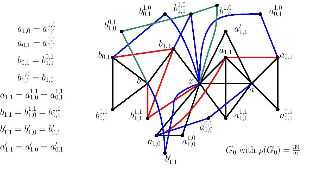
Figure 1.

We first prove the claim in (i), in the following lemma:

Lemma 5.1.

The graph $G_{0}$ in Figure 1 is strictly balanced.

Proof.

Observe that $G_{0}$ can be split into two edge-disjoint parts having only $x$ in common, illustrated in Figure 2.

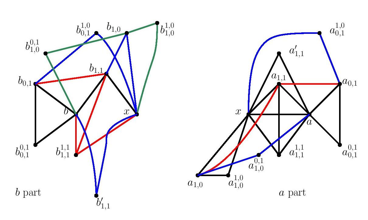
Figure 2.

The vertices in the $a$ part can be added in the following sequence:

1. in step $0$, the vertex $x$,

2. in step $1$, the vertex $a$, bringing $1$ edge,

3. in step $2$, the vertices $a^{\prime}_{1,1}$ and $a_{1,1}$, each bringing precisely $2$ edges,

4. in step $3$, the vertices $a_{1,0}$ and $a_{0,1}$, each bringing precisely $2$ edges,

5. in step $4$, the vertices $a_{1,0}^{1,0}$, $a_{0,1}^{0,1}$, $a_{1,0}^{0,1}$ and $a_{0,1}^{1,0}$, each bringing precisely $2$ edges,

6. in step $5$, the vertex $a_{1,1}^{1,1}$, bringing $3$ edges.

The vertices in the $b$ part can be added in the following sequence:

1. in step $0$, the vertex $x$,

2. in step $1$, the vertex $b_{1,1}$, bringing $1$ edge,

3. in step $2$, the vertices $b_{1,1}^{1,1}$ and $b_{1,0}$, each bringing $2$ edges,

4. in step $3$, the vertices $b$ and $b_{1,0}^{1,0}$, each bringing $2$ edges,

5. in step $4$, the vertices $b_{0,1}$, $b^{\prime}_{1,1}$, $b_{1,0}^{0,1}$, each bringing $2$ edges,

6. in step $5$, the vertices $b_{0,1}^{1,0}$ and $b_{0,1}^{0,1}$, each bringing $2$ edges.

If we consider a subgraph $H$ of $G_{0}$ containing $x$, $a$, $b_{1,1}$, and $y_{i}$ vertices from step $i$ of $a$ part and $z_{i}$ vertices from step $i$ of $b$ part for $i\in\{2,3,4,5\}$, with $y_{2},y_{3},z_{2},z_{3},z_{5}\in\{0,1,2\}$, $y_{4},z_{4}\in\{0,1,2,3,4\}$ and $y_{5}\in\{0,1\}$, the number of edges in $H$ is at most $1+2\sum_{i=2}^{4}(y_{i}+z_{i})+3y_{5}+2z_{5},$ whereas the number of vertices is $3+\sum_{i=2}^{5}(y_{i}+z_{i})$. Letting $y=\sum_{i=2}^{4}(y_{i}+z_{i})+z_{5}$ and $z=y_{5}$, $\rho(H)$ is at most

$$\frac{1+2y+3z}{3+y+z}.$$ (5.4)

We note here that

$$\frac{3+2y+3z}{4+y+z}-\frac{1+2y+3z}{3+y+z} =\frac{5-z}{(4+y+z)(3+y+z)},$$

which is positive since $z\leq 1$. Thus the density increases with $y$. Similarly, the density increases with $z$. Thus $\rho(H)<\rho(G_{0})$ whenever $H$ is a proper subgraph of $G_{0}$ containing $x$, $a$, $b_{1,1}$. When $H$ excludes at least one of $x$, $a$ and $b_{1,1}$, its density is even lower, since in both $a$ and $b$ parts, the vertex added in step $2$ brings $1$ edge, and subsequent vertices bring at most $2$ edges each, except possibly for $a_{1,1}^{1,1}$ if it is included in $H$.

∎

The first part of (ii) is trivial. The appropriate values of $v(G_{0})$, $e(G_{0})$ and $\rho(G_{0})$ are given in Figure 1. We now prove the second part of (ii). For $\varphi$ to be true on a graph $G$, the bare minimum we need are the following vertices, edges and non-edges in $G$:

1. $x$, $a$, $b$ where $x\sim a$ and $b\nsim x$;

2. $a_{1,1}$ with $a_{1,1}\sim x$, $a_{1,1}\sim a$;

3. $a_{1,0}$ with $a_{1,0}\sim x$ and $a_{1,0}\nsim a$;

4. $a_{1,1}^{1,1}$ with $a_{1,1}^{1,1}\sim x$, $a_{1,1}^{1,1}\sim a$ and $a_{1,1}^{1,1}\sim a_{1,1}$;

5. $a^{\prime}_{1,1}$ with $a^{\prime}_{1,1}\sim x$, $a^{\prime}_{1,1}\sim a$, $a^{\prime}_{1,1}\nsim a_{1,1}$;

6. $a_{1,0}^{1,0}$ with $a_{1,0}^{1,0}\sim x$, $a_{1,0}^{1,0}\sim a_{1,0}$ and $a_{1,0}^{1,0}\nsim a$;

7. $b_{0,1}$ with $b_{0,1}\sim b$, $b_{0,1}\nsim x$;

8. $b_{0,1}^{0,1}$ with $b_{0,1}^{0,1}\sim b$, $b_{0,1}^{0,1}\sim b_{0,1}$ and $b_{0,1}^{0,1}\nsim x$.

Let us call this subgraph $H$ with $v(H)=10$ and $e(H)=14$ (see Figure 3).

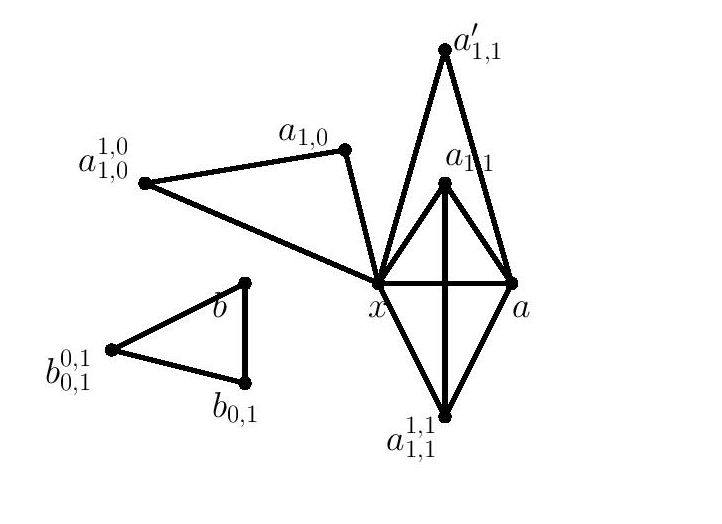
Figure 3.

The set of variables left to evaluate is

$$S_{0}=\Big{\{}b_{1,1},a_{0,1},a_{0,1}^{0,1},a_{1,1}^{1,0},a_{1,1}^{0,1},a_{1,0}^{1,1},a^{\prime}_{1,0},a_{1,0}^{0,1},a_{0,1}^{1,1},a^{\prime}_{0,1},a_{0,1}^{1,0},b_{1,1}^{1,1},b^{\prime}_{1,1},b_{1,1}^{1,0},b_{1,1}^{0,1},b_{1,0},b_{1,0}^{1,1},b^{\prime}_{1,0},\\ b_{1,0}^{1,0},b_{1,0}^{0,1},b_{0,1}^{1,1},b^{\prime}_{0,1},b_{0,1}^{1,0}\Big{\}}.$$ (5.5)

In what follows, we consider a family $\Sigma$ of finite graphs $\Gamma$ with at most $43$ vertices, adding vertices evaluating the elements of $S_{0}$ to $H$, such that if $G\models\varphi$, it contains an induced subgraph isomorphic to some $\Gamma\in\Sigma$. We show that $\operatorname{\rho_{\max}}(\Gamma)>\rho(G_{0})$ for each $\Gamma\in\Sigma\setminus G_{0}$ by considering various scenarios, the most difficult of which is discussed in Subsection 5.1 below, and the rest in the Appendix (Section 6). The notation introduced below, unless otherwise stated, will be used in the Appendix.

5.1. The most difficult scenario:

Here we assume that $a_{0,1}$ and $a_{0,1}^{0,1}$ are added as new vertices to $H$, thus yielding the graph $H_{0}$ as in Figure 4, with $17$ edges and $12$ vertices.

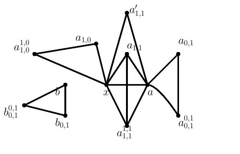
Figure 4.

Either $b_{1,1}$ is a new vertex added to $H_{0}$, in which case we add edges $\{b_{1,1},x\}$ and $\{b_{1,1},b\}$, or it belongs to

$$S_{1}=\left\{a,a_{1,0},a_{1,1},a_{1,1}^{1,1},a^{\prime}_{1,1},a_{1,0}^{1,0}\right\},$$ (5.6)

in which case we add $\{b_{1,1},b\}$. We denote by $H^{\prime}_{0}$ the graph obtained after accounting for $b_{1,1}$. We define the vertices:

1. $v_{1}$ is adjacent to all of $x$, $b$ and $b_{0,1}$,

2. $v_{2}$ is adjacent to all of $x$, $b$ and $b_{1,1}$,

3. $v_{3}$ is adjacent to all of $x$, $a$ and $a_{1,0}$,

4. $v_{4}$ is adjacent to all of $x$, $a$ and $a_{0,1}$,

and we call them the first-level vertices. We call a first-level vertex old if it coincides with a vertex in $H^{\prime}_{0}$, we call it unique if it is added as a new vertex to $H^{\prime}_{0}$ and does not coincide with any other first-level vertex, and banal otherwise. The graph obtained after we have accounted for all first-level vertices is denoted $H_{1}$. We define the vertices:

1. $u_{1}$ is adjacent to $x$ and $b_{0,1}$, non-adjacent to $b$,

2. $u_{2}$ is adjacent to $x$ and $b$, non-adjacent to $b_{1,1}$,

3. $u_{3}$ is adjacent to $b$ and $b_{1,1}$, non-adjacent to $x$,

4. $u_{4}$ is adjacent to $x$ and $b_{1,1}$, non-adjacent to $b$,

5. $u_{5}$ is adjacent to $a$ and $a_{1,0}$, non-adjacent to $x$,

6. $u_{6}$ is adjacent to $x$ and $a_{1,1}$, non-adjacent to $a$,

7. $u_{7}$ is adjacent to $a$ and $a_{1,1}$, non-adjacent to $x$,

8. $u_{8}$ is adjacent to $x$ and $a_{0,1}$, non-adjacent to $a$.

We call these second-level vertices. We call a second-level vertex old if it coincides with a vertex in $H^{\prime}_{0}$, we call it banal if it coincides with a first-level vertex that is not old (in other words, coincides with a vertex in $V(H_{1})\setminus V\left(H^{\prime}_{0}\right)$), and we call it unique otherwise. Note that two or more unique second-level vertices are allowed to coincide with each other.

Remark 5.2.

Note that we have not yet considered a vertex evaluating $b_{1,0}$, its “extensions” which are vertices evaluating $b_{1,0}^{1,1}$, $b^{\prime}_{1,0}$, $b_{1,0}^{1,0}$, $b_{1,0}^{0,1}$, as well as $b^{\prime}_{0,1}$, $a^{\prime}_{0,1}$ and $a^{\prime}_{1,0}$. As it happens, some of these end up coinciding with some of the vertices in Figure 1.

If $v_{3}$ is old, it either coincides with a vertex in

$$S_{2}=\left\{a_{1,1},a_{1,1}^{1,1},a^{\prime}_{1,1}\right\},$$ (5.7)

in which case we add $\{v_{3},a_{1,0}\}$, or $v_{3}=b_{1,1}$ when $b_{1,1}\in V\left(H^{\prime}_{0}\right)\setminus V(H_{0})$, in which case we add $\{b_{1,1},a\}$ and $\{b_{1,1},a_{1,0}\}$. When $v_{4}$ is old, either $v_{4}\in S_{2}$, in which case we add $\{v_{4},a_{0,1}\}$, or with $b_{1,1}$ when $b_{1,1}\in V\left(H^{\prime}_{0}\right)\setminus V(H_{0})$, in which case we add $\{b_{1,1},a\}$ and $\{b_{1,1},a_{0,1}\}$. When $v_{1}$ is old and coincides with $b_{1,1}$, we add $\{b_{1,1},b_{0,1}\}$; if $v_{1}\in S_{1}\setminus\{b_{1,1}\}$, we add $\{v_{1},b\}$ and $\{v_{1},b_{0,1}\}$. When $v_{2}$ is old, the possibilities according to $b_{1,1}$ are:

1. if $b_{1,1}\in V\left(H^{\prime}_{0}\right)\setminus V(H_{0})$, and $v_{2}\in S_{1}$, we add $\{v_{2},b\}$ and $\{v_{2},b_{1,1}\}$;

2. if $b_{1,1}=a_{1,0}$, and $v_{2}=a_{1,0}^{1,0}$, we add $\{a_{1,0}^{1,0},b\}$; if $v_{2}\neq a_{1,0}^{1,0}$, we add $\{v_{2},a_{1,0}\}$ and $\{v_{2},b\}$;

3. if $b_{1,1}=a_{1,0}^{1,0}$ and $v_{2}=a_{1,0}$, we add $\{a_{1,0},b\}$; if $v_{2}\neq a_{1,0}$, we add $\{v_{2},a_{1,0}^{1,0}\}$ and $\{v_{2},b\}$;

4. if $b_{1,1}=a_{1,1}$ and $v_{2}\in\{a_{1,0},a_{1,0}^{1,0}\}$, we add $\{v_{2},b\}$ and $\{v_{2},a_{1,1}\}$; if $v_{2}\in\{a,a_{1,1}^{1,1}\}$, we add $\{v_{2},b\}$;

5. if $b_{1,1}=a_{1,1}^{1,1}$ and $v_{2}\in\{a_{1,0},a^{\prime}_{1,1},a_{1,0}^{1,0}\}$, we add $\{v_{2},b\}$ and $\{v_{2},a_{1,1}^{1,1}\}$; if $v_{2}\in\{a,a_{1,1}\}$, we add $\{v_{2},b\}$;

6. if $b_{1,1}=a^{\prime}_{1,1}$ and $v_{2}\in\{a_{1,1}^{1,1},a_{1,0},a_{1,0}^{1,0}\}$, we add $\{v_{2},b\}$ and $\{v_{2},a^{\prime}_{1,1}\}$; if $v_{2}=a$, we add $\{v_{2},b\}$;

7. if $b_{1,1}=a$, then $v_{2}\in S_{2}$, and we add $\{v_{2},b\}$.

Lemma 5.3.

Suppose $\nu_{1}$ is the number of new, distinct first-level vertices (including both unique and banal ones) that are added to $H^{\prime}_{0}$. Then the number of edges that we need to add on account of all first-level vertices is at least $2\nu_{1}+5$ when $b_{1,1}\in V\left(H^{\prime}_{0}\right)\setminus V(H_{0})$ and $v_{2}$ is old; in all other cases, this number is at least $2\nu_{1}+4$.

Proof.

When $b_{1,1}\in V\left(H^{\prime}_{0}\right)\setminus V(H_{0})$ and both $v_{2}$ and $v_{3}$ are old, they bring edges $\{b_{1,1},a\}$, $\{b_{1,1},a_{1,0}\}$, $\{a_{1,0},b\}$ when $v_{2}=a_{1,0}$ and $v_{3}=b_{1,1}$, or edges $\{v_{3},a_{1,0}\}$, $\{v_{2},b\}$, $\{v_{2},b_{1,1}\}$ when $v_{3}\neq b_{1,1}$, and $4$ edges otherwise. If $v_{2}$ is old and $v_{3}$ is not, then $v_{2}$ brings edges $\{v_{2},b\}$ and $\{v_{2},b_{1,1}\}$. If $v_{1}$ is old, it brings $\{v_{1},b_{0,1}\}$; if $v_{4}$ is old, it brings $\{v_{4},a_{0,1}\}$. This shows that the number of edges added due to old first-level vertices is at least one more than the number of old first-level vertices when $v_{2}$ is old.

When $b_{1,1}\in V\left(H^{\prime}_{0}\right)\setminus V(H_{0})$ but $v_{2}$ is not old, we get $\{v_{3},a_{1,0}\}$ when $v_{3}$ is old, $\{v_{4},a_{0,1}\}$ when $v_{4}$ is old, $\{v_{1},b_{0,1}\}$ when $v_{1}$ is old; when $b_{1,1}\in V(H_{0})$, we additionally get $\{v_{2},b\}$ when $v_{2}$ is old. Since $\{v_{1},b_{0,1}\}$, $\{v_{2},b\}$, $\{v_{3},a_{1,0}\}$ and $\{v_{4},a_{0,1}\}$ are all distinct, hence the number of edges added due to old first-level vertices bring is at least as large as the number of old first-level vertices here.

Whether $b_{1,1}\in V\left(H^{\prime}_{0}\right)\setminus V(H_{0})$ or not, any $2$ first-level vertices coinciding in a banal vertex bring at least $4$ edges, any $3$ coinciding in a banal vertex bring at least $5$ edges, and all $4$ coinciding in a banal vertex bring at least $6$ edges. This concludes the proof.

∎

Lemma 5.4.

If $s$ banal second-level vertices coincide with a first-level vertex $v_{i}$, except for when $u_{2}$ and $v_{1}$ coincide, at least $s$ additional edges are introduced due to these second-level vertices. If $s$ many unique second-level vertices coincide with each other, they together bring at least $s+1$ edges.

Proof.

The only second-level vertices that can coincide with $v_{1}$ are $u_{2}$, $u_{6}$ and $u_{8}$: when $v_{1}=u_{2}$, we add no edge; when $v_{1}=u_{6}$, we add $\{v_{1},a_{1,1}\}$; when $v_{1}=u_{8}$, we add $\{v_{1},a_{0,1}\}$. The only second-level vertices that can coincide with $v_{2}$ are $u_{6}$ and $u_{8}$: when $v_{2}=u_{6}$, we add $\{v_{2},a_{1,1}\}$; when $v_{2}=u_{8}$, we add $\{v_{2},a_{0,1}\}$. The only second-level vertices that can coincide with $v_{i}$, for $i\in\{3,4\}$, are $u_{1}$, $u_{2}$ and $u_{4}$: when $v_{i}=u_{1}$, we add $\{v_{i},b_{0,1}\}$; when $v_{i}=u_{2}$, we add $\{v_{i},b\}$; when $v_{i}=u_{4}$, we add $\{v_{i},b_{1,1}\}$. This proves the first part of Lemma 5.4.

Some or all of $u_{3}$, $u_{5}$ and $u_{7}$ may coincide (and none of them may coincide with any other second-level vertex) – $u_{3}$ brings $\{u_{3},b\}$ and $\{u_{3},b_{1,1}\}$, $u_{5}$ brings $\{u_{5},a\}$ and $\{u_{5},a_{1,0}\}$ and $u_{7}$ brings $\{u_{7},a\}$ and $\{u_{7},a_{1,1}\}$. Of these, only $\{u_{5},a\}$ and $\{u_{7},a\}$ coincide if $u_{5}=u_{7}$. Among the remaining vertices $u_{1}$, $u_{2}$, $u_{4}$, $u_{6}$ and $u_{8}$, there are two inclusion-maximum sets $\left\{u_{1},u_{4},u_{6},u_{8}\right\}$ and $\left\{u_{2},u_{6},u_{8}\right\}$ that may coincide. In the former case, $u_{6}$ brings $\{u_{6},a_{1,1}\}$, $u_{8}$ brings $\{u_{8},a_{0,1}\}$, $u_{1}$ brings $\{u_{1},b_{0,1}\}$ and $u_{4}$ brings $\{u_{4},b_{1,1}\}$, which are all distinct; additionally, the common vertex is adjacent to $x$. In the latter case, $u_{6}$ brings $\{u_{6},a_{1,1}\}$, $u_{8}$ brings $\{u_{8},a_{0,1}\}$ and $u_{2}$ brings $\{u_{2},b\}$, which are all distinct; additionally, the common vertex is adjacent to $x$. ∎

Let $\nu_{2}$ denote the number of unique second-level vertices we add to the graph $H_{1}$ and $e$ the number of edges that are added to $H_{1}$ due to non-unique second-level vertices. Let the graph obtained after accounting for all second-level vertices be denoted $H_{2}$.

5.1.1. First subcase:

We consider $b_{1,1}\in V\left(H^{\prime}_{0}\right)\setminus V(H_{0})$ and $v_{2}$ not old. If the first-level vertices bring precisely $2\nu_{1}+4$ edges together, and each distinct, unique second-level vertex brings precisely $2$ edges, then $\rho(H_{2})$ is at least

$$\frac{17+2+(2\nu_{1}+4)+2\nu_{2}+e}{12+1+\nu_{1}+\nu_{2}}=\frac{23+2(\nu_{1}+\nu_{2})+e}{13+(\nu_{1}+\nu_{2})}.$$ (5.8)

For this to be strictly less than $\frac{13}{7}$, we require $(\nu_{1}+\nu_{2})+7e<8$. Thus, either $e=1$ and $\nu_{1}+\nu_{2}=0$, which is not possible since $\nu_{1}+\nu_{2}=0$ implies $\nu_{1}=0$, which implies that $v_{2}$ is old, contradicting our hypothesis, or else $e=0$ and $\nu_{1}+\nu_{2}\leq 7$. In what follows, no two unique second-level vertices are allowed to coincide, nor any banal second-level vertex allowed to exist except when $v_{1}$ is not old and $v_{1}=u_{2}$, because of Lemma 5.4. We now split the analysis into a few cases depending on the value of $\nu_{1}$, keeping in mind that $v_{2}$ is not old:

1. When $\nu_{1}=1$, so that $\nu_{2}\leq 6$: First, suppose all of $v_{1},v_{3},v_{4}$ are old – they together bring precisely $3$ edges only when $v_{3},v_{4}\in S_{2}$ and $v_{1}=b_{1,1}$, and these edges are $\{v_{3},a_{1,0}\}$, $\{v_{4},a_{0,1}\}$, and $\{v_{1},b_{0,1}\}=\{b_{1,1},b_{0,1}\}$; the edge incident on $b_{1,1}$ and added due to $v_{2}$ is $\{v_{2},b_{1,1}\}$. In $H_{1}$, the only neighbours of $a_{1,0}$ are $x$, $a_{1,0}^{1,0}$ and $v_{3}$, so that there exists no vertex that can play the role of $u_{5}$; the only neighbours of $b_{0,1}$ are $b$, $b_{0,1}^{0,1}$ and $v_{1}$, so that no vertex plays the role of $u_{1}$; the only neighbours of $a_{0,1}$ are $a$, $a_{0,1}^{0,1}$ and $v_{4}$, so that no vertex plays the role of $u_{8}$; the only neighbours of $b_{1,1}$ are $x$, $b$ and $v_{2}$, so that no vertex plays the role of $u_{4}$; the only common neighbours of $x$ and $b$ are $b_{1,1}$ and $v_{2}$, so that no vertex plays the role of $u_{2}$. Thus $u_{1}$, $u_{2}$, $u_{4}$, $u_{5}$, $u_{8}$ need to be added as distinct, unique second-level vertices.

   When not all of $v_{1},v_{3},v_{4}$ are old, in addition to $u_{1}$, $u_{2}$, $u_{4}$, $u_{5}$, $u_{8}$, we need to add at least one of $u_{3}$, $u_{6}$, $u_{7}$ as a unique, distinct second-level vertices (note that if $v_{1}$ is not old, it coincides with $v_{2}$ since $\nu_{1}=1$, hence $u_{2}$ cannot coincide with $v_{1}$).

   When $v_{1},v_{3},v_{4}$ are old, we have room to add one new vertex and $2$ new edges to $H_{2}$; when $v_{1},v_{3},v_{4}$ are not all old, we can neither add a new vertex nor a new edge to $H_{2}$. We now consider all the possibilities for $b_{1,0}$:

   • If $b_{1,0}$ coincides with $a_{1,0}$, since the only neighbours of $a_{1,0}$ are $x$, $a_{1,0}^{1,0}$ and $v_{3}$, hence no vertex in $H_{2}$ can play the role of $b_{1,0}^{1,1}$ or $b_{1,0}^{0,1}$ without adding further edges. We thus have to add both of these as new vertices.

   • If $b_{1,0}$ coincides with $u_{1}$, since the only neighbours of $u_{1}$ are $x$ and $b_{0,1}$, hence no vertex in $H_{2}$ can play the role of $b_{1,0}^{1,1}$ or $b_{1,0}^{1,0}$ without adding further edges. We thus have to add both of these as new vertices.

   • If $b_{1,0}$ coincides with $u_{4}$, since the only neighbours of $u_{4}$ are $b_{1,1}$ and $x$, hence no vertex in $H_{2}$ can play the role of $b_{1,0}^{1,0}$ or $b_{1,0}^{0,1}$ without adding further edges. We thus have to add both of these as new vertices.

   • If we add $b_{1,0}$ as a new vertex, it brings precisely $1$ edge, and we are allowed to add one more edge but no new vertices. This is not enough to account for all of $b_{1,0}^{1,1}$, $b_{1,0}^{1,0}$ and $b_{1,0}^{0,1}$.

   Thus it never suffices to add a single new vertex and $2$ new edges to $H_{2}$, thus violating the condition $\nu_{2}\leq 6$.

2. When $\nu_{1}=2$: In this case, we need $\nu_{2}\leq 5$. If $v_{3}$ and $v_{4}$ are old, the only neighbours to $b_{1,1}$ in $H_{1}$ are $x$, $b$ and $v_{2}$, so that no vertex in $H_{1}$ plays the role of $u_{3}$ nor of $u_{4}$. If $v_{3}$ and $v_{1}$ are old, the only neighbours of $a_{1,1}$ are $x$, $a$, $a_{1,1}^{1,1}$ and possibly $a_{1,0}$ if $v_{3}=a_{1,1}$, so that no vertex in $H_{1}$ plays the role of $u_{7}$. If $v_{4}$ and $v_{1}$ are old, the only neighbours of $a_{1,1}$ are $x$, $a$, $a_{1,1}^{1,1}$ and possibly $a_{0,1}$ if $v_{4}=a_{1,1}$, so that no vertex in $H_{1}$ plays the role of $u_{6}$. Moreover, as in (i), all of $u_{1}$, $u_{5}$, $u_{4}$, $u_{8}$ need to be added as unique, distinct second-level vertices in each of the above cases; when $v_{1}$ and $v_{3}$ are old or $v_{1}$ and $v_{4}$ are old, we also need to add $u_{2}$ as a new vertex. Clearly, this forces $\nu_{2}\geq 6$. If less than $2$ first-level vertices are old, even more second-level vertices need to be added as unique, distinct second-level vertices.

3. When $\nu_{1}\geq 3$: In this case, we need $\nu_{2}\leq 4$. We argue as above that $u_{1}$, $u_{5}$, $u_{4}$, $u_{8}$ all need to be added as unique, distinct second-level vertices. If $v_{1}$ is old, then both $u_{6}$ and $u_{7}$ need to be added as distinct, unique second-level vertices; if $v_{3}$ or $v_{4}$ is old, we add both $u_{3}$ and $u_{4}$ as new second-level vertices. All these show that $u\leq 4$ is a condition that clearly cannot be met.

5.1.2. Second subcase:

We consider $b_{1,1}\in V\left(H^{\prime}_{0}\right)\setminus V(H_{0})$ and $v_{2}$ old. By Lemma 5.3, the number of edges added due to all first-level vertices is $2\nu_{1}+5$. Since each distinct unique second-level vertex brings at least $2$ edges, $\rho(H_{2})$ is at least

$$\frac{17+2+(2\nu_{1}+5)+2\nu_{2}+e}{12+1+\nu_{1}+\nu_{2}}=\frac{24+2(\nu_{1}+\nu_{2})+e}{13+(\nu_{1}+\nu_{2})},$$ (5.9)

and for this to be strictly less than $\frac{13}{7}$, we require $\nu_{1}+\nu_{2}+7e<1$, implying $\nu_{1}=\nu_{2}=e=0$. From the proof of Lemma 5.3, we note that the number of edges contributed by all $4$ old first-level vertices is precisely $5$ only under one of the following situations.

If $v_{2}=a_{1,0}$ and $v_{3}=b_{1,1}$, the edges due to first-level vertices are $\{b_{1,1},a\}$, $\{b_{1,1},a_{1,0}\}$, $\{a_{1,0},b\}$, $\{v_{1},b_{0,1}\}$ and $\{v_{4},a_{0,1}\}$ (if $v_{1}\neq b_{1,1}$, then we must have $v_{1}=a_{1,0}$). Note that the only neighbours of $b_{0,1}$ in $H_{1}$ are $b$, $b_{0,1}^{0,1}$ and $v_{1}$, all of which are adjacent to $b$, so that no vertex in $H_{1}$ plays the role of $u_{1}$. Thus we have to add $u_{1}$ as a unique second-level vertex, thus violating the required condition $\nu_{2}=0$.

If $v_{3}\neq b_{1,1}$, the edges due to first-level vertices are $\{v_{3},a_{1,0}\}$, $\{v_{2},b\}$, $\{v_{2},b_{1,1}\}$, $\{v_{1},b_{0,1}\}$ and $\{v_{4},a_{0,1}\}$ (if $v_{1}\neq b_{1,1}$, then we must have $v_{1}=v_{2}$). Once again, $u_{1}$ needs to be added as a unique second-level vertex, violating $\nu_{2}=0$.

5.1.3. Third subcase:

When $b_{1,1}\in V(H_{0})$, if each unique second-level vertex brings precisely $2$ edges, $\rho(H_{2})$ is at least

$$\frac{17+1+(2\nu_{1}+4)+2\nu_{2}+e}{12+\nu_{1}+\nu_{2}}=\frac{22+2(\nu_{1}+\nu_{2})+e}{12+(\nu_{1}+\nu_{2})}.$$ (5.10)

For this to be strictly less than $\frac{13}{7}$, we require $(\nu_{1}+\nu_{2})+7e<2$, forcing $e=0$ and $\nu_{1}+\nu_{2}\leq 1$. The only neighbours of $a_{0,1}$ in $H_{1}$ are $a$, $a_{0,1}^{0,1}$ and $v_{4}$, and the only neighbours to $b_{0,1}$ are $b$, $b_{0,1}^{0,1}$ and $v_{1}$, so that there exist no vertices playing the roles of $u_{8}$ and $u_{1}$. Since both $u_{1}$ and $u_{8}$ need to be added as unique second-level vertices, they must coincide, but by Lemma 5.4, the common vertex will bring $3$ edges instead of precisely $2$.

5.2. Showing that for $\alpha<\frac{7}{13}$, zero-one law for $\mathcal{E}_{4}$ holds for $\left\{G(n,n^{-\alpha})\right\}_{n}$:

For $\alpha<\frac{7}{13}$, when $G_{1}\sim G(m,m^{-\alpha})$ and $G_{2}\sim G(n,n^{-\alpha})$ are independent, we show that a.a.s. Duplicator wins $\operatorname{EHR}[G_{1},G_{2},4]$. Let Spoiler play on $G_{1}$ and Duplicator on $G_{2}$ without loss of generality, and the vertices picked in $G_{1}$ are denoted $x_{i}$ and in $G_{2}$ by $y_{i}$, for $i\in[4]$. A.a.s. as $m,n\rightarrow\infty$, both $G_{1}$ and $G_{2}$ contain induced subgraphs isomorphic to $G_{0}$, and Duplicator makes use of the copy of $G_{0}$ present inside $G_{2}$ in her winning strategy. Given our description of $G_{0}$, it is clear, for the most part (in particular, for the first $2$ rounds), how Duplicator responds to Spoiler while playing on the copy of $G_{0}$ inside $G_{2}$. We point out here some of the less obvious responses.

Lemma 5.5.

A.a.s. for every subgraph of $G_{2}$ that is isomorphic to $G_{0}$, and whose vertices are named the same as the corresponding vertices of $G_{0}$, there exist the following vertices, edges and non-edges in $G_{2}$:

1. vertex $c$ that is non-adjacent to $x$, $a$ and $a^{\prime}_{1,1}$ but adjacent to $a_{1,1}$;

2. vertex $c^{1,0}$ that is adjacent to $c$ and $x$ but not to $a$;

3. vertex $c^{0,1}$ that is adjacent to $c$ and $a$ but not to $x$.

4. vertex $d$ that is non-adjacent to $x$, $b$ and $b^{\prime}_{1,1}$ but adjacent to $b_{1,1}$;

5. vertex $d^{1,0}$ that is adjacent to $d$ and $x$ but not to $b$;

6. vertex $d^{0,1}$ that is adjacent to $d$ and $b$ but not to $x$.

Proof.

Let $H$ be the induced subgraph on $x,a,a_{1,1},a^{\prime}_{1,1}$ and $G$ that on $x,a,a_{1,1},a^{\prime}_{1,1},c,c^{1,0},c^{0,1}$ in $G_{2}$ such that $E(G)\setminus E(H)$ comprises precisely the edges and non-edges described in the statement of Lemma 5.5. Consider $H\subset S\subseteq G$ with $c\in S$. It is straightforward to see that $e(S,H)$ is at most $\frac{5}{3}$ times $v(S,H)$, and hence $f_{\alpha}(S,H)>0$ for $\alpha<\frac{7}{13}$. The argument is similar for the vertices $d$, $d^{1,0}$ and $d^{0,1}$. From Theorem 2.5, the rest follows.

∎

Suppose Spoiler picks $x_{3}$ that is non-adjacent to $x_{1}$ and $x_{2}$ – then Duplicator sets $y_{3}=c$ if $y_{2}=a$, and $y_{3}=d$ otherwise (i.e. if $y_{2}=b$). If Spoiler selects $x_{4}$ that is adjacent to $x_{1},x_{2},x_{3}$, then Duplicator sets $y_{4}=a_{1,1}$ if $y_{2}=a$, and $y_{4}=b_{1,1}$ otherwise. If Spoiler selects $x_{4}$ that is adjacent to $x_{1}$, $x_{2}$ but not to $x_{3}$, Duplicator sets $y_{4}=a^{\prime}_{1,1}$ when $y_{2}=a$ and $y_{4}=b^{\prime}_{1,1}$ otherwise. If Spoiler selects $x_{4}$ that is adjacent to $x_{1}$, $x_{3}$ but not to $x_{2}$, then Duplicator sets $y_{4}=c^{1,0}$ when $y_{2}=a$ and $y_{4}=d^{1,0}$ otherwise. If Spoiler selects $x_{4}$ that is adjacent to $x_{2}$, $x_{3}$ but not to $x_{1}$, then Duplicator sets $y_{4}=c^{0,1}$ when $y_{2}=a$ and $y_{4}=d^{0,1}$ otherwise. Finally, no matter what $x_{1},x_{2},x_{3}$ may have been, suppose Spoiler selects $x_{4}$ that is adjacent to at most one of $x_{1},x_{2},x_{3}$. If $G$ is the subgraph of $G_{1}$ induced on $\{x_{1},x_{2},x_{3},x_{4}\}$ and $H$ that on $\{x_{1},x_{2},x_{3}\}$, the pair $(G,H)$ is $\alpha$-safe for all $\alpha<1$ – hence, by Theorem 2.5, Duplicator a.a.s. finds $y_{4}$ in $G_{2}$ such that $y_{4}\sim y_{i}$ iff $x_{4}\sim x_{i}$ for $i\in[3]$.

6. Appendix

Here we compile the remaining cases to complete the proof of (ii) of Section 5. At the very outset, we recall the sets $S_{1}$ and $S_{2}$ defined in (5.6) and (5.7) respectively. In Remarks 6.1 through 6.5, we collect all the possibilities for $b_{1,1}$ and the first-level vertices that we consider in § 6.1 through § 6.12.

Remark 6.1.

If $b_{1,1}\in V\left(H^{\prime}_{0}\right)\setminus V(H_{0})$, we add edges $\{b_{1,1},x\}$ and $\{b_{1,1},b\}$, and if $b_{1,1}\in S_{1}\setminus\{a\}$, we add $\{b_{1,1},b\}$. In § 6.1, § 6.2, § 6.3, § 6.5, § 6.7 and § 6.11, we do not add any edge if $b_{1,1}=a$, otherwise we add edge $\{a,b\}$.

Remark 6.2.

In § 6.2 and § 6.5, we do not consider $v_{1}$ at all, whereas in § 6.4, § 6.6, § 6.8 and § 6.12, we do not consider $v_{1}$ when $b_{1,1}=a$, since in all these scenarios, $a$ plays the role of $v_{1}$. What follows excludes these cases. If $v_{1}\in S_{1}\setminus\{a,b_{1,1}\}$, we add edges $\{v_{1},b\}$ and $\{v_{1},b_{0,1}\}$, and if $v_{1}=b_{1,1}$, we add $\{b_{1,1},b_{0,1}\}$. In § 6.1, § 6.3, § 6.7 and § 6.11, we add edge $\{a,b_{0,1}\}$ when $v_{1}=a$, in § 6.4, § 6.6, § 6.8 and § 6.12, we add edge $\{a,b\}$ when $v_{1}=a$, and in § 6.9 and § 6.10, we add both $\{a,b\}$ and $\{a,b_{0,1}\}$ when $v_{1}=a$.

Remark 6.3.

In § 6.1, § 6.2, § 6.3, § 6.5, § 6.7 and § 6.11, we do not consider $v_{2}$ whenever $b_{1,1}\in S_{2}$, since $a$ plays the role of $v_{2}$; moreover, in these subsections, we add only edge $\{a,b_{1,1}\}$ whenever $b_{1,1}\in V\left(H^{\prime}_{0}\right)\setminus V(H_{0})$ and $v_{2}=a$. For all other cases, we have:

1. if $b_{1,1}\in V\left(H^{\prime}_{0}\right)\setminus V(H_{0})$, $v_{2}\in S_{1}$ and we add $\{v_{2},b\}$ and $\{v_{2},b_{1,1}\}$;

2. if $b_{1,1}=a$, $v_{2}\in S_{2}$ and we add $\{v_{2},b\}$;

3. if $b_{1,1}=a_{1,1}$, either $v_{2}\in\left\{a,a_{1,1}^{1,1}\right\}$ and add $\{v_{2},b\}$, or $v_{2}\in\left\{a_{1,0},a_{1,0}^{1,0}\right\}$ and we add $\{v_{2},a_{1,1}\}$ and $\{v_{2},b\}$;

4. if $b_{1,1}=a_{1,1}^{1,1}$, either $v_{2}\in\left\{a,a_{1,1}\right\}$ and add $\{v_{2},b\}$, or $v_{2}\in\left\{a^{\prime}_{1,1},a_{1,0},a_{1,0}^{1,0}\right\}$ and we add $\{v_{2},b\}$ and $\left\{v_{2},a_{1,1}^{1,1}\right\}$;

5. if $b_{1,1}=a^{\prime}_{1,1}$, either $v_{2}=a$ and we add $\{a,b\}$, or $v_{2}\in\left\{a_{1,1}^{1,1},a_{1,0},a_{1,0}^{1,0}\right\}$ and add $\{v_{2},b\}$ and $\{v_{2},a^{\prime}_{1,1}\}$;

6. if $b_{1,1}=a_{1,0}$, either $v_{2}=a_{1,0}^{1,0}$ and we add $\left\{a_{1,0}^{1,0},b\right\}$, or $v_{2}\in S_{2}$ and we add $\{v_{2},a_{1,0}\}$ and $\{v_{2},b\}$;

7. if $b_{1,1}=a_{1,0}^{1,0}$, either $v_{2}=a_{1,0}$ and we add $\{a_{1,0},b\}$, or $v_{2}\in S_{2}$ and we add $\left\{v_{2},a_{1,0}^{1,0}\right\}$ and $\{v_{2},b\}$.

Remark 6.4.

If $v_{3}$ is old, either $v_{3}\in S_{2}$, in which case we add the edge $\{v_{3},a_{1,0}\}$, or else $v_{3}=b_{1,1}$ when $b_{1,1}\in V\left(H^{\prime}_{0}\right)\setminus V(H_{0})$, and we add the edges $\{b_{1,1},a\}$ and $\{b_{1,1},a_{1,0}\}$.

Remark 6.5.

In § 6.1, § 6.2 and § 6.3, we do not consider $v_{4}$ whenever $b_{1,1}\in S_{2}$, since $b_{1,1}$ plays the role of $v_{4}$. In all other cases, if $v_{4}\in S_{2}$ and we add edge $\{v_{4},b\}$ in § 6.1 through § 6.3, $\{v_{4},b_{0,1}\}$ in § 6.4 through § 6.6, $\{v_{4},a_{0,1}\}$ in § 6.7 through § 6.9, and $\left\{v_{4},b_{0,1}^{0,1}\right\}$ in § 6.10 through § 6.12. If $b_{1,1}\in V\left(H^{\prime}_{0}\right)\setminus V(H_{0})$ and $v_{4}=b_{1,1}$, we add only the edge $\{a,b_{1,1}\}$ in § 6.1 through § 6.3, edges $\{a,b_{1,1}\}$ and $\{b_{1,1},b_{0,1}\}$ in § 6.4 through § 6.6, edges $\{a,b_{1,1}\}$ and $\{b_{1,1},a_{0,1}\}$ in § 6.7 through § 6.9, and edges $\{a,b_{1,1}\}$ and $\left\{b_{1,1},b_{0,1}^{0,1}\right\}$ in § 6.10 through § 6.12.

6.1. Second case:

Here we assume that $a_{0,1}=b$ and $a_{0,1}^{0,1}$ is added as a new vertex; we then add edges $\{a,b\}$, $\left\{b,a_{0,1}^{0,1}\right\}$, $\left\{a_{0,1}^{0,1},a\right\}$ to get $H_{0}$ in Figure 5 with $17$ edges and $11$ vertices. We split the analysis according to $b_{1,1}$.

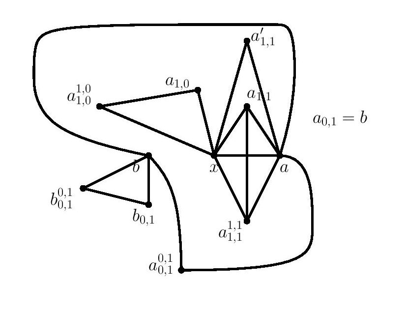
Figure 5.

6.1.1. When $b_{1,1}\in V\left(H^{\prime}_{0}\right)\setminus V(H_{0})$:

Neither the edge $\left\{v_{3},a_{1,0}\right\}$ that is added due to an old $v_{3}$ nor the edge $\{v_{1},b_{0,1}\}$ added due to an old $v_{1}$ coincides with any other edge added due to old first-level vertices. Only when $v_{2}$ and $v_{4}$ are simultaneously old and $v_{2}=a$ and $v_{4}=b_{1,1}$, a single edge is added due to $2$ old first-level vertices. If $2$ first-level vertices are banal and coincide, the common vertex brings at least $4$ edges; if $3$ of them are banal and coincide, the common vertex brings at least $5$ edges; if all of them are banal and coincide, the common vertex brings at least $6$ edges.

As before, $\nu_{1}$ denotes the number of distinct new first-level vertices. When $\nu_{1}\leq 2$, the number of edges added due to all first-level vertices is $2\nu_{1}+3$ and not higher only if both $v_{2}$ and $v_{4}$ are old with $v_{2}=a$ and $v_{4}=b_{1,1}$, and either $v_{1}$ is new or $v_{1}\in\{a,b_{1,1}\}$ (if not, we get two edges $\{v_{1},b\}$ and $\{v_{1},b_{0,1}\}$ from $v_{1}$, making the number of edges due to all first-level vertices at least $2\nu_{1}+4$). Therefore, in $H_{1}$, the graph obtained after accounting for all first-level vertices, $b_{0,1}$ has neighbours $b$, $b_{0,1}^{0,1}$ and $v_{1}$, so that there exists no vertex in $H_{1}$ that is adjacent to $x$ and $b_{0,1}$ but not to $b$. Similarly, $a_{1,0}$ has neighbours $x$, $a_{1,0}^{1,0}$ and $v_{3}$, so that there exists no vertex in $H_{1}$ that is adjacent to $a$ and $a_{1,0}$ but not to $x$. Hence the second-level vertices $u_{1}$ and $u_{5}$ cannot be found in $H_{1}$ without adding further edges. Now, the density of $H_{2}$, the graph obtained after accounting for all second-level vertices, is

$$\rho(H_{2})\geq\frac{17+2+(2\nu_{1}+3)+2\nu_{2}+e}{11+1+\nu_{1}+\nu_{2}}=\frac{22+2(\nu_{1}+\nu_{2})+e}{12+(\nu_{1}+\nu_{2})},$$ (6.1)

and for this to be less than $\frac{13}{7}$, we require $(\nu_{1}+\nu_{2})+7e<2$, which implies $e=0$ and $\nu_{1}+\nu_{2}\leq 1$. The condition $e=0$ implies both $u_{1}$ and $u_{5}$ need to be added as unique second-level vertices, and the condition $\nu_{1}+\nu_{2}\leq 1$ implies that at most one of them can be added as a unique second-level vertex. Thus we arrive at a contradiction.

When $\nu_{1}\geq 3$, the number of edges added due to all first-level vertices is at least $2\nu_{1}+4$, making $\rho(H_{2})$ at least

$$\frac{17+2+2\nu_{1}+4+2\nu_{2}+e}{11+1+\nu_{1}+\nu_{2}}=\frac{23+2(\nu_{1}+\nu_{2})+e}{12+(\nu_{1}+\nu_{2})}\geq\frac{23}{12}>\frac{13}{7}.$$ (6.2)

6.1.2. When $b_{1,1}=a$:

Once again, neither edge $\{v_{3},a_{1,0}\}$ added if $v_{3}$ is old nor edge $\{v_{1},b_{0,1}\}$ added if $v_{1}$ is old coincides with any other edge added due to old first-level vertices. When $v_{2}$ and $v_{4}$ are both old and $v_{2}=v_{4}=v$, a single edge $\{v,b\}$ is added due to them.

If $v_{2}$ and $v_{4}$ are banal and coincide, the common vertex is adjacent to $x$, $b$, $a$; any other pair of coinciding banal first-level vertices bring at least $4$ edges. If $v_{1},v_{2},v_{4}$ are banal and coincide, the common vertex is adjacent to $x$, $b$, $b_{0,1}$, $a$; if $v_{2},v_{3},v_{4}$ are banal and coincide, the common vertex is adjacent to $x$, $b$, $a$, $a_{1,0}$; all other triplets of coinciding banal first-level vertices bring at least $5$ edges. If $v_{1},v_{2},v_{3},v_{4}$ are banal and coincide, the common vertex is adjacent to $x$, $b$, $b_{0,1}$, $a$, $a_{1,0}$.

These show that the number of edges added due to all first-level vertices is $2\nu_{1}+3$ and not higher when $\nu_{1}\leq 3$, $v_{2}$ and $v_{4}$ coincide, whether banal or old, and $v_{1}$ is either new or $v_{1}=a$ or $v_{1}=v_{2}=v_{4}$. Thus

$$\rho(H_{2})\geq\frac{17+(2\nu_{1}+3)+2\nu_{2}+e}{11+\nu_{1}+\nu_{2}}=\frac{20+2(\nu_{1}+\nu_{2})+e}{11+(\nu_{1}+\nu_{2})},$$ (6.3)

and for this to be less than $\frac{13}{7}$, we need $(\nu_{1}+\nu_{2})+7e<3$, which implies $e=0$ and $\nu_{1}+\nu_{2}\leq 2$. In $H_{1}$, the only neighbours of $b_{0,1}$ are $b$, $b_{0,1}^{0,1}$ and $v_{1}$, so that no vertex plays the role of $u_{1}$; the only neighbours of $a_{1,0}$ are $x$, $a_{1,0}^{1,0}$ and $v_{3}$, so that no vertex plays the role of $u_{5}$; the only neighbours of $b$ are $b_{0,1}$, $b_{0,1}^{0,1}$, $a_{0,1}^{0,1}$, $a$ and $v$, where $v_{2}=v_{4}=v$ either belongs to $S_{2}$ or to $V\left(H_{1}\right)\setminus V\left(H^{\prime}_{0}\right)$, and hence there exists no vertex in $H_{1}$ that plays the role of $u_{8}$ which is adjacent to $x$ and $a_{0,1}=b$ but not to $a$. Thus none of $u_{1}$, $u_{5}$, $u_{8}$ can be found in $H_{1}$ without adding further edges. The condition $e=0$ implies that all of them need to be added as unique second-level vertices, which violates the condition $\nu_{1}+\nu_{2}\leq 2$.

When $\nu_{1}=4$, we get at least $12$ edges, making $\rho(H_{2})$ at least

$$\frac{17+12+2\nu_{2}+e}{11+4+\nu_{2}}=\frac{29+2\nu_{2}+e}{15+\nu_{2}}\geq\frac{29}{15}>\frac{13}{7}.$$ (6.4)

6.1.3. When $b_{1,1}=a_{1,0}$:

Any two old first-level vertices bring at least $2$ edges. If $v_{2},v_{3},v_{4}$ are old, they bring $2$ edges and not more only if $v_{2}=v_{3}=v_{4}=v$ for some $v\in S_{2}$, and these edges are $\{v,b\}$ and $\{v,a_{1,0}\}$. Any other triplet of old first-level vertices bring at least $3$ edges. If all first-level vertices are old, they bring $3$ edges and not more only in the following two scenarios: i) either $v_{2}=v_{3}=v_{4}=v_{1}=v$ for some $v\in S_{2}$, and the edges added are $\{v,b\}$, $\{v,a_{1,0}\}$ and $\{v,b_{0,1}\}$; ii) or $v_{2}=v_{3}=v_{4}=v$ for some $v\in S_{2}$ and $v_{1}\in\{a,a_{1,0}\}$, and the edges added are $\{v,b\}$, $\{v,a_{1,0}\}$ and $\{v_{1},b_{0,1}\}$. Any $2$ coinciding banal first-level vertices bring at least $4$ edges; if $v_{2}$, $v_{3}$ and $v_{4}$ are banal and coincide, the common vertex is adjacent to $x$, $a$, $b$, $a_{1,0}$, whereas any other triplet of coinciding banal first-level vertices bring at least $5$ edges; if all are banal and coincide, the common vertex is adjacent to $x$, $a$, $b$, $a_{1,0}$ and $b_{0,1}$. Thus the first-level vertices contribute at least $2\nu_{1}+3$ edges when $\nu_{1}\leq 2$ and at least $2\nu_{1}+4$ when $\nu_{1}\geq 3$, making $\rho(H_{2})$ at least

$$\frac{17+1+2\nu_{1}+3+2\nu_{2}+e}{11+\nu_{1}+\nu_{2}}=\frac{21+2(\nu_{1}+\nu_{2})+e}{11+(\nu_{1}+\nu_{2})}\geq\frac{21}{11}>\frac{13}{7}.$$ (6.5)

6.1.4. When $b_{1,1}=a_{1,0}^{1,0}$:

The edge $\{v_{3},a_{1,0}\}$ is added when $v_{3}$ is old; the edge $\{v_{1},b_{0,1}\}$ is added when $v_{1}$ is old; the edge $\{v_{4},b\}$ is added when $v_{4}$ is old. These edges are all distinct (even if $v_{1}=a_{1,0}$, the edges $\{v_{3},a_{1,0}\}$ and $\{v_{1},b_{0,1}\}$ do not coincide since $v_{3}\in S_{2}$ and thus $v_{3}\neq b_{0,1}$). Finally, if $v_{2}\in S_{2}$, it brings both the edges $\{v_{2},b\}$ and $\left\{v_{2},a_{1,0}^{1,0}\right\}$, so that even if $v_{2}=v_{4}$, the edge $\left\{v_{2},a_{1,0}^{1,0}\right\}$ does not coincide with any of the previously mentioned edges; if $v_{2}=a_{1,0}$, it brings edge $\{a_{1,0},b\}$, which does not coincide with $\{v_{4},b\}$ since $v_{4}\in S_{2}$, does not coincide with $\{v_{3},a_{1,0}\}$ since $v_{3}\in S_{2}$, and clearly $\{v_{1},b_{0,1}\}\neq\{a_{1,0},b\}$.

The number of edges added due to all first-level vertices is at least $2\nu_{1}+4$, so that

$$\rho(H_{2})\geq\frac{17+1+(2\nu_{1}+4)+2\nu_{2}+e}{11+\nu_{1}+\nu_{2}}=\frac{22+2(\nu_{1}+\nu_{2})+e}{11+(\nu_{1}+\nu_{2})}\geq 2>\frac{13}{7}.$$ (6.6)

6.1.5. When $b_{1,1}\in S_{2}$:

Here we only consider $v_{1}$ and $v_{3}$. The number of edges due to them is $2\nu_{1}+2$ and not higher only if $v_{1}$ is new of $v_{1}\in\left\{a,b_{1,1}\right\}$, giving us the edges $\{v_{1},b_{0,1}\}$ and $\{v_{3},a_{1,0}\}$. Then

$$\rho(H_{2})\geq\frac{17+1+(2\nu_{1}+2)+2\nu_{2}+e}{11+\nu_{1}+\nu_{2}}=\frac{20+2(\nu_{1}+\nu_{2})+e}{11+(\nu_{1}+\nu_{2})}.$$ (6.7)

For this to be less than $\frac{13}{7}$, we need $\nu_{1}+\nu_{2}+7e<3$, implying that $\nu_{1}+\nu_{2}\leq 2$ and $e=0$. The only neighbours of $b_{0,1}$ in $H_{1}$ are $b$, $b_{0,1}^{0,1}$ and $v_{1}$; the only neighbours of $a_{1,0}$ in $H_{1}$ are $x$, $a_{1,0}^{1,0}$ and $v_{3}$; the only common neighbours of $x$ and $b$ in $H_{1}$ are $b_{1,1}$ and $a$. Thus there exist no vertices in $H_{1}$ that play the roles of $u_{1}$, $u_{5}$ and $u_{2}$ without adding further edges, forcing us to add them as distinct unique second-level vertices and violating the condition $\nu_{1}+\nu_{2}\leq 2$.

6.2. Third case:

We assume that $a_{0,1}=b$ and $a_{0,1}^{0,1}=b_{0,1}$, and add edges $\{a,b\}$ and $\left\{a,b_{0,1}\right\}$ to get $H_{0}$ in Figure 6 with $16$ edges and $10$ vertices.

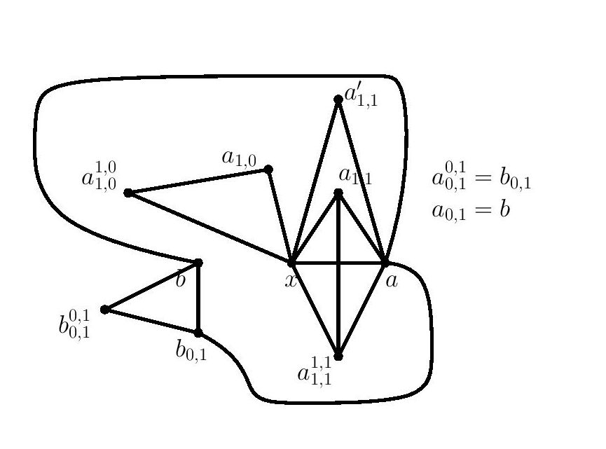
Figure 6.

6.2.1. When $b_{1,1}\in V\left(H^{\prime}_{0}\right)\setminus V(H_{0})$:

The only scenario where $2$ old first-level vertices contribute a single edge is when $v_{4}=b_{1,1}$ and $v_{2}=a$ and this edge is $\{a,b_{1,1}\}$; if old, $v_{3}$ brings at least the edge $\{v_{3},a_{1,0}\}$. Any $2$ coinciding banal first-level vertices bring at least $4$ edges; if all $3$ are banal and coincide, they bring $6$ edges. Thus the first-level vertices contribute $2\nu_{1}+2$ edges and no more only when $\nu_{1}\leq 1$ and $v_{2}=a$, $v_{4}=b_{1,1}$, making $\rho(H_{2})$ at least

$$\frac{16+2+2\nu_{1}+2+2\nu_{2}+e}{10+1+\nu_{1}+\nu_{2}}=\frac{20+2(\nu_{1}+\nu_{2})+e}{11+(\nu_{1}+\nu_{2})},$$ (6.8)

which is less than $\frac{13}{7}$ only if $(\nu_{1}+\nu_{2})+7e<3$, implying $e=0$ and $\nu_{1}+\nu_{2}\leq 2$. The only neighbours of $a_{1,0}$ in $H_{1}$ are $x$, $a_{1,0}^{1,0}$ and $v_{3}$; the only neighbours of $b_{0,1}$ in $H_{1}$ are $a$, $b$ and $b_{0,1}^{0,1}$; the only common neighbours of $x$ and $b$ are $b_{1,1}$ and $a$ with $a\sim b_{1,1}$ in $H_{1}$. Thus there exist no vertices in $H_{1}$ playing the roles of $u_{1}$, $u_{5}$ and $u_{2}$, requiring them to be added as distinct unique second-level vertices, violating $\nu_{1}+\nu_{2}\leq 2$. When $\nu_{1}\geq 2$, we get at least $2\nu_{1}+3$ edges from first-level vertices, making $\rho(H_{2})\geq\frac{21}{11}>\frac{13}{7}$.

6.2.2. When $b_{1,1}=a$:

The edge added due to $v_{2}$ being old is $\{v_{2},b\}$, that due to $v_{3}$ being old is $\{v_{3},a_{1,0}\}$, and that due to $v_{4}$ being old is $\{v_{4},b\}$. If $v_{2}$ and $v_{4}$ are banal and coincide, the common vertex is adjacent to $x$, $b$, $a$; if $v_{2},v_{3},v_{4}$ are banal and coincide, the common vertex is adjacent to $x$, $b$, $a$, $a_{1,0}$. The first-level vertices thus contribute $2\nu_{1}+2$ edges and no more only when $v_{2}=v_{4}$, whether old or banal. Thus

$$\rho(H_{2})\geq\frac{16+2\nu_{1}+2+2\nu_{2}+e}{10+\nu_{1}+\nu_{2}}=\frac{18+2(\nu_{1}+\nu_{2})+e}{10+(\nu_{1}+\nu_{2})},$$ (6.9)

which is less than $\frac{13}{7}$ only if $(\nu_{1}+\nu_{2})+7e<4$, implying $e=0$ and $\nu_{1}+\nu_{2}\leq 3$. The only neighbours of $b_{0,1}$ in $H_{1}$ are $b$, $b_{0,1}^{0,1}$ and $a$, where both $b_{0,1}^{0,1}$ and $a$ are adjacent to $b$, hence there exists no vertex in $H_{1}$ playing the role of $u_{1}$. The only neighbours of $a_{1,0}$ are $x$, $a_{1,0}^{1,0}$ and $v_{3}$, where both $a_{1,0}^{1,0}$ and $v_{3}$ are adjacent to $x$, hence there exists no vertex in $H_{1}$ playing the role of $u_{5}$. The only common neighbours of $x$ and $b$ in $H_{1}$ are $a$ and $v_{2}=v_{4}$ which is adjacent to $b_{1,1}=a$, and hence there exists no vertex in $H_{1}$ playing the role of $u_{2}$. Since $u_{1}$, $u_{2}$, $u_{5}$ need to be added as distinct unique second-level vertices, all first-level vertices and all other second-level vertices must be old.

The only way both $u_{6}$ and $u_{7}$ are old is if $v_{2}=v_{3}=v_{4}=a_{1,1}$, in which case $u_{6}=a_{1,0}$ and $u_{7}=b$; also, $u_{3}=b_{0,1}$ and $u_{4}\in\left\{a^{\prime}_{1,1},a_{1,1}^{1,1}\right\}$ will work, whereas $u_{8}=u_{2}$. We must have $b_{1,0}\in\left\{a^{\prime}_{1,1},a_{1,1}^{1,1},a_{1,0},a_{1,0}^{1,0},u_{1}\right\}$. If $b_{1,0}=a^{\prime}_{1,1}$, its neighbours are $x$ and $a$, and if $b_{1,0}=a_{1,1}^{1,1}$, its neighbours are $x$, $a$ and $a_{1,1}$, hence there exist no vertices in $H_{2}$ playing the roles of $b_{1,0}^{1,0}$ and $b_{1,0}^{0,1}$. If $b_{1,0}=a_{1,0}$, its neighbours are $u_{5}$, $a_{1,1}$, $x$ and $a_{1,0}^{1,0}$, there exists no vertex playing the role of $b_{1,0}^{0,1}$. If $b_{1,0}=a_{1,0}^{1,0}$, its neighbours are $x$ and $a_{1,0}$, hence there exist no vertices playing the roles of $b_{1,0}^{1,1}$ and $b_{1,0}^{0,1}$. If $b_{1,0}=u_{1}$, its neighbours are $x$ and $b_{0,1}$, hence there exist no vertices playing the roles of $b_{1,0}^{1,1}$ and $b_{1,0}^{1,0}$.

6.2.3. When $b_{1,1}=a_{1,0}$:

The first-level vertices contribute $2\nu_{1}+2$ edges only if $v_{2}=v_{3}=v_{4}$, whether old or banal; else at least $2\nu_{1}+3$ edges. Thus

$$\rho(H_{2})\geq\frac{16+1+(2\nu_{1}+2)+2\nu_{2}+e}{10+\nu_{1}+\nu_{2}}=\frac{19+2(\nu_{1}+\nu_{2})+e}{10+\nu_{2}}\geq\frac{19}{10}>\frac{13}{7}.$$ (6.10)

6.2.4. When $b_{1,1}=a_{1,0}^{1,0}$:

The first-level vertices contribute at least $2\nu_{1}+3$ edges, so that

$$\rho(H_{2})\geq\frac{16+1+2\nu_{1}+3+2\nu_{2}+e}{10+\nu_{1}+\nu_{2}}=\frac{20+2(\nu_{1}+\nu_{2})+e}{10+(\nu_{1}+\nu_{2})}\geq 2>\frac{13}{7}.$$ (6.11)

6.2.5. When $b_{1,1}\in S_{2}$:

We only consider $v_{3}$, which, if old, brings $1$ edge, and if new, brings $3$ edges. In the former scenario, if each unique second-level vertex brings precisely $2$ edges, we have

$$\rho(H_{2})\geq\frac{16+1+1+2\nu_{2}+e}{10+\nu_{2}}=\frac{18+2\nu_{2}+e}{10+\nu_{2}}.$$ (6.12)

For this to be less than $\frac{13}{7}$, we need $\nu_{2}+7e<4$, implying $e=0$ and $\nu_{2}\leq 3$. As above, we argue that $u_{1}$, $u_{2}$, $u_{5}$ need to be added as distinct, unique second-level vertices, which leaves no room for any other new vertex nor new edge. If $u_{6}$ and $u_{7}$ are to exist in $H_{1}$, we need $b_{1,1}=v_{3}=a_{1,1}$, giving $u_{6}=a_{1,0}$ and $u_{7}=b$; we set $u_{8}=u_{2}$ and $u_{4}=a_{1,1}^{1,1}$. But the only common neighbour of $b$ and $b_{1,1}=a_{1,1}$ in $H_{1}$ is $a$, which is adjacent to $x$, hence $u_{3}$ needs to be added as a unique second-level vertex. If $u_{3}$ coincides with $u_{5}$, then the common unique second-level vertex brings $4$ edges, which violates our assumption above.

When $v_{3}$ is a unique first-level vertex,

$$\rho(H_{2})\geq\frac{16+1+3+2\nu_{2}+e}{10+1+\nu_{2}}=\frac{20+2\nu_{2}+e}{11+\nu_{2}}.$$ (6.13)

For this to be less than $\frac{13}{7}$, we need $\nu_{2}+7e<3$, forcing $e=0$ and $\nu_{2}\leq 2$. As above, we need to add $u_{1}$, $u_{2}$, $u_{5}$ as distinct, unique second-level vertices, violating the condition $\nu_{2}\leq 2$.

6.3. Fourth case:

We assume that $a_{0,1}=b$ and $a_{0,1}^{0,1}=b_{0,1}^{0,1}$, adding edges $\left\{a,b\right\}$ and $\left\{a,b_{0,1}^{0,1}\right\}$ to get$H_{0}$ in Figure 7 with $16$ edges and $10$ vertices.

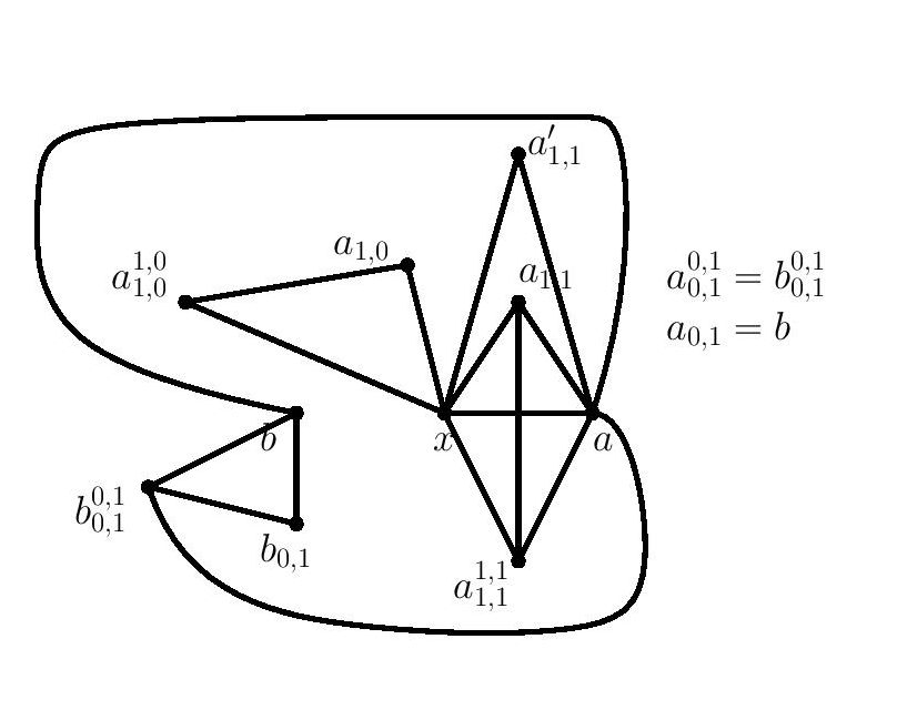
Figure 7.

6.3.1. When $b_{1,1}\in V\left(H^{\prime}_{0}\right)\setminus V(H_{0})$:

We add at least the edge $\{v_{3},a_{1,0}\}$ when $v_{3}$ is old, at least the edge $\{v_{1},b_{0,1}\}$ when $v_{1}$ is old, and these are distinct from any other edge added due to old first-level vertices. When $v_{2}$ and $v_{4}$ are both old, they together bring a single edge and not more only when $v_{2}=a$ and $v_{4}=b_{1,1}$. Any $2$ coinciding banal first-level vertices bring at least $4$ edges, any $3$ at least $5$, and when all $4$ are banal and coincide, $6$ edges. Thus the first-level vertices contribute at least $2\nu_{1}+3$ edges (at least $2\nu_{1}+4$ when $\nu_{1}\geq 3$), making $\rho(H_{2})$ at least

$$\frac{16+2+(2\nu_{1}+3)+2\nu_{2}+e}{10+1+\nu_{1}+\nu_{2}}=\frac{21+2(\nu_{1}+\nu_{2})+e}{11+(\nu_{1}+\nu_{2})}\geq\frac{21}{11}>\frac{13}{7}.$$ (6.14)

6.3.2. When $b_{1,1}=a$:

Once again, the edge $\{v_{3},a_{1,0}\}$ added when $v_{3}$ is old and the edge $\{v_{1},b_{0,1}\}$ added when $v_{1}$ is old are distinct from all other edges added due to old first-level vertices. When $v_{2}$ and $v_{4}$ are old, they together bring a single edge and not more only when $v_{2}=v_{4}=v$ for some $v\in S_{2}$. If $v_{2}$ and $v_{4}$ are banal and coincide, the common vertex is adjacent to $x$, $b$, $a$; any other pair of coinciding banal first-level vertices bring at least $4$ edges; any $3$ coinciding banal first-level vertices which include both $v_{2}$ and $v_{4}$ bring $4$ edges, else at least $5$ edges; if all $4$ are banal and coincide, they bring $5$ edges. The first-level vertices thus bring at least $2\nu_{1}+3$ edges when $\nu_{1}\leq 3$, and $12$ edges when $\nu_{1}=4$, making

$$\rho(H_{2})\geq\frac{16+(2\nu_{1}+3)+2\nu_{2}+e}{10+\nu_{1}+\nu_{2}}=\frac{19+2(\nu_{1}+\nu_{2})+e}{10+(\nu_{1}+\nu_{2})}\geq\frac{19}{10}>\frac{13}{7}.$$ (6.15)

6.3.3. When $b_{1,1}=a_{1,0}$:

If $v_{2}$, $v_{3}$, $v_{4}$ are old, they bring $2$ edges and no more only if $v_{2}=v_{3}=v_{4}=v$ for some $v\in S_{2}$; we add at least the edge $\{v_{1},b_{0,1}\}$ when $v_{1}$ is old. If $v_{2}$, $v_{3}$, $v_{4}$ are banal and coincide, the common vertex is adjacent to $x$, $b$, $a_{1,0}$, $a$. Any other triplet of coinciding banal first-level vertices bring at least $5$ edges; any pair of coinciding banal first-level vertices bring at least $4$ edges; when all $4$ are banal and coincide, we get $5$ edges. Thus the first-level vertices bring at least $2\nu_{1}+3$ edges when $\nu_{1}\leq 2$ and at least $2\nu_{1}+4$ edges when $\nu_{1}\geq 3$, making

$$\rho(H_{2})\geq\frac{16+1+(2\nu_{1}+3)+2\nu_{2}+e}{10+\nu_{1}+\nu_{2}}=\frac{20+2(\nu_{1}+\nu_{2})+e}{10+(\nu_{1}+\nu_{2})}\geq 2>\frac{13}{7}.$$ (6.16)

6.3.4. When $b_{1,1}=a_{1,0}^{1,0}$:

If $v_{2}$ is old and equals $a_{1,0}$, and $v_{4}$ is old, note that the edges $\{a_{1,0},b\}$ and $\{v_{4},b\}$ cannot coincide as $v_{4}\in S_{2}$; similarly, if $v_{3}$ is old, $\{v_{3},a_{1,0}\}$ does not coincide with $\{a_{1,0},b\}$ as $v_{3}\in S_{2}$. The first-level vertices bring at least $2\nu_{1}+4$ edges, making

$$\rho(H_{2})\geq\frac{16+1+(2\nu_{1}+4)+2\nu_{2}+e}{10+\nu_{1}+\nu_{2}}=\frac{21+2(\nu_{1}+\nu_{2})+e}{10+(\nu_{1}+\nu_{2})}>2>\frac{13}{7}.$$ (6.17)

6.3.5. When $b_{1,1}\in S_{2}$:

The first-level vertices bring at least $2\nu_{1}+2$ edges, hence

$$\rho(H_{2})\geq\frac{16+1+2\nu_{1}+2+2\nu_{2}+e}{10+\nu_{1}+\nu_{2}}=\frac{19+2(\nu_{1}+\nu_{2})+e}{10+(\nu_{1}+\nu_{2})}\geq\frac{19}{10}>\frac{13}{7}.$$ (6.18)

6.4. Fifth case:

Here we assume that $a_{0,1}=b_{0,1}$ and add $a_{0,1}^{0,1}$ as a new vertex, along with edges $\{a,b_{0,1}\}$, $\left\{b_{0,1},a_{0,1}^{0,1}\right\}$ and $\left\{a_{0,1}^{0,1},a\right\}$ to get $H_{0}$ in Figure 8 with $17$ edges and $11$ vertices.

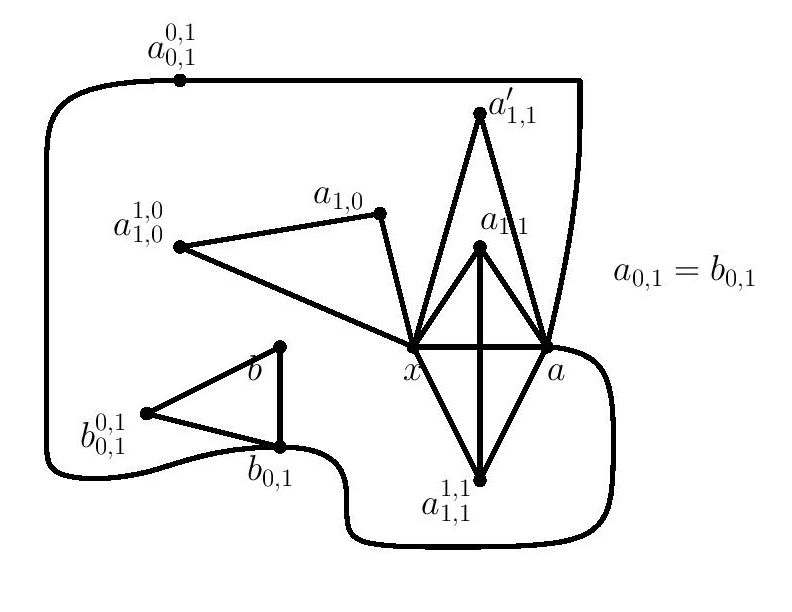
Figure 8.

6.4.1. When $b_{1,1}\in V\left(H^{\prime}_{0}\right)\setminus V(H_{0})$:

When $v_{3}$ is old, it brings at least the edge $\{v_{3},a_{1,0}\}$, which coincides with no other edge added due to old first-level vertices except possibly $\{v_{2},b_{1,1}\}$ if $v_{2}=a_{1,0}$ and $v_{3}=b_{1,1}$, but then we additionally get the edges $\{a_{1,0},b\}$ and $\{a,b_{1,1}\}$. When $v_{1}$ and $v_{2}$ are old, we get edges $\{a,b\}$ and $\{a,b_{1,1}\}$ when $v_{1}=v_{2}=a$, and at least $3$ edges otherwise; when $v_{1}$ and $v_{4}$ are old, we get edges $\{v,b\}$ and $\{v,b_{0,1}\}$ when $v_{1}=v_{4}=v$ for some $v\in S_{2}$, or $\{v_{4},b_{0,1}\}$ and $\{a,b\}$ when $v_{4}\in S_{2}$ and $v_{1}=a$, or $\{a,b_{1,1}\}$ and $\{b_{1,1},b_{0,1}\}$ when $v_{1}=v_{4}=b_{1,1}$, and at least $3$ edges otherwise. All other pairs of old first-level vertices bring at least $2$ edges. When $v_{1}$, $v_{2}$, $v_{3}$ are old, we get edges $\{a,b\}$, $\{a,b_{1,1}\}$ and $\{b_{1,1},a_{1,0}\}$ when $v_{1}=v_{2}=a$ and $v_{3}=b_{1,1}$, or $\{a,b\}$, $\{a,b_{1,1}\}$ and $\{v_{3},a_{1,0}\}$ when $v_{1}=v_{2}=a$ and $v_{3}\in S_{2}$, and at least $3$ edges otherwise. When $v_{1}$, $v_{2}$, $v_{4}$ are old, we get edges $\{a,b\}$, $\{a,b_{1,1}\}$ and $\{v_{4},b_{0,1}\}$ when $v_{1}=v_{2}=a$ and $v_{4}\in S_{2}$, or $\{v,b\}$, $\{v,b_{0,1}\}$ and $\{v,b_{1,1}\}$ when $v_{1}=v_{2}=v_{4}=v$ for some $v\in S_{2}$, or $\{a,b\}$, $\{a,b_{1,1}\}$ and $\{b_{1,1},b_{0,1}\}$ when $v_{1}=v_{2}=a$ and $v_{4}=b_{1,1}$, and at least $4$ edges otherwise. When $v_{1}$, $v_{3}$, $v_{4}$ are old, we get edges $\{b_{1,1},b_{0,1}\}$, $\{a,b_{1,1}\}$ and $\{b_{1,1},a_{1,0}\}$ when $v_{1}=v_{3}=v_{4}=b_{1,1}$, or $\{b_{1,1},b_{0,1}\}$, $\{a,b_{1,1}\}$ and $\{v_{3},a_{1,0}\}$ when $v_{1}=v_{4}=b_{1,1}$ and $v_{3}\in S_{2}$, $\{v,b\}$, $\{v,b_{0,1}\}$ and $\{v_{3},a_{1,0}\}$ when $v_{1}=v_{4}=v$ for some $v\in S_{2}$ and $v_{3}\in S_{2}$, or $\{v_{4},b_{0,1}\}$, $\{v_{3},a_{1,0}\}$ and either $\{b_{1,1},b_{0,1}\}$ or $\{a,b\}$ when $v_{4}\in S_{2}$, $v_{3}\in S_{2}$ and $v_{1}$ is either $b_{1,1}$ or $a$. When $v_{2}$, $v_{3}$, $v_{4}$ are old, they bring at least $4$ edges. When all $4$ are old, they bring at least $4$ edges.

Any $2$ coinciding banal first-level vertices bring at least $4$ edges, any $3$ bring at least $5$ edges, and when all $4$ are banal and coincide, they bring $6$ edges. Thus the first-level vertices bring at least $2\nu_{1}+4$ edges, so that

$$\rho(H_{2})\geq\frac{17+2+(2\nu_{1}+4)+2\nu_{2}+e}{11+1+\nu_{1}+\nu_{2}}=\frac{23+2(\nu_{1}+\nu_{2})+e}{12+(\nu_{1}+\nu_{2})}\geq\frac{23}{13}>\frac{13}{7}.$$ (6.19)

6.4.2. When $b_{1,1}=a_{1,1}$:

When $v_{1}$ and $v_{2}$ are old, we get edge $\{a,b\}$ if $v_{1}=v_{2}=a$, and at least $2$ edges otherwise; when $v_{1}$ and $v_{4}$ are old, we get $\{a_{1,1},b_{0,1}\}$ if $v_{1}=v_{4}=a_{1,1}$, and at least $2$ edges otherwise. Any other pair of old first-level vertices bring at least $2$ edges. When $v_{1}$, $v_{2}$, $v_{3}$ are old, they bring edges $\{a,b\}$ and $\{v_{3},a_{1,0}\}$ when $v_{1}=v_{2}=a$, and at least $3$ edges otherwise. When $v_{1}$, $v_{2}$, $v_{4}$ are old, they bring edges $\{a,b\}$ and $\{v_{4},b_{0,1}\}$ when $v_{1}=v_{2}=a$, edges $\left\{a_{1,1}^{1,1},b\right\}$ and $\left\{a_{1,1}^{1,1},b_{0,1}\right\}$ when $v_{1}=v_{2}=v_{4}=a_{1,1}^{1,1}$, edges $\{a_{1,1},b_{0,1}\}$ and $\{v_{2},b\}$ when $v_{1}=v_{4}=a_{1,1}$ and $v_{2}\in\left\{a,a_{1,1}^{1,1}\right\}$, and at least $3$ edges otherwise. When $v_{1}$, $v_{3}$, $v_{4}$ are old, they bring edges $\{a_{1,1},b_{0,1}\}$ and $\{v_{3},a_{1,0}\}$ if $v_{1}=v_{4}=a_{1,1}$, and at least $3$ edges otherwise. When $v_{2},v_{3},v_{4}$ are old, we get at least $3$ edges. When all $4$ are old, we get at least $3$ edges. Contributions from banal first-level vertices is the same as in § 6.4.1. The first-level vertices thus contribute at least $2\nu_{1}+3$ edges when $\nu_{1}\leq 2$ and at least $2\nu_{1}+4$ edges when $\nu_{1}\geq 3$, making

$$\rho(H_{2})\geq\frac{17+1+(2\nu_{1}+3)+2\nu_{2}+e}{11+\nu_{1}+\nu_{2}}=\frac{21+2(\nu_{1}+\nu_{2})+e}{11+\nu_{1}+\nu_{2}}\geq\frac{21}{11}>\frac{13}{7}.$$ (6.20)

6.4.3. When $b_{1,1}\in\left\{a_{1,1}^{1,1},a^{\prime}_{1,1}\right\}$:

The analysis is mutatis mutandis to § 6.4.2.

6.4.4. When $b_{1,1}=a_{1,0}$:

Any $2$ old first-level vertices bring at least $2$ edges, any $3$ bring at least $3$ edges; when all $4$ are old, they bring edges $\{v,a_{1,0}\}$, $\{v,b_{0,1}\}$ and $\{v,b\}$ only if $v_{1}=v_{2}=v_{3}=v_{4}=v$ for some $v\in S_{2}$, and at least $4$ edges otherwise. Any $2$ coinciding banal first-level vertices bring at least $4$ edges, any $3$ bring at least $5$ edges, and when all $4$ are banal and coincide, the common vertex is adjacent to $x$, $b$, $b_{0,1}$, $a_{1,0}$, $a$. The first-level vertices cotntribute at least $2\nu_{1}+3$ edges when $\nu_{1}\leq 1$, and at least $2\nu_{1}+4$ edges when $\nu_{1}\geq 2$, so that

$$\rho(H_{2})\geq\frac{17+1+(2\nu_{1}+3)+2\nu_{2}+e}{11+\nu_{1}+\nu_{2}}=\frac{21+2(\nu_{1}+\nu_{2})+e}{11+\nu_{1}+\nu_{2}}\geq\frac{21}{11}>\frac{13}{7}.$$ (6.21)

6.4.5. When $b_{1,1}=a_{1,0}^{1,0}$:

The first-level vertices bring at least $2\nu_{1}+4$ edges, so that

$$\rho(H_{2})\geq\frac{17+1+(2\nu_{1}+4)+2\nu_{2}+e}{11+\nu_{1}+\nu_{2}}=\frac{22+2(\nu_{1}+\nu_{2})+e}{11+(\nu_{1}+\nu_{2})}\geq 2>\frac{13}{7}.$$ (6.22)

6.4.6. When $b_{1,1}=a$:

The first-level vertices bring at least $2\nu_{1}+3$ edges, so that

$$\rho(H_{2})\geq\frac{17+1+(2\nu_{1}+3)+2\nu_{2}+e}{11+\nu_{1}+\nu_{2}}=\frac{21+2(\nu_{1}+\nu_{2})+e}{11+\nu_{1}+\nu_{2}}\geq\frac{21}{11}>\frac{13}{7}.$$ (6.23)

6.5. Sixth case:

We assume here that $a_{0,1}=b_{0,1}$ and $a_{0,1}^{0,1}=b$, and add $\{a,b\}$ and $\{a,b_{0,1}\}$, to get $H_{0}$ in Figure 9 with $16$ edges and $10$ vertices.

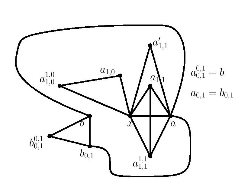
Figure 9.

6.5.1. When $b_{1,1}\in V\left(H^{\prime}_{0}\right)\setminus V(H_{0})$:

We add edge $\{v_{3},a_{1,0}\}$ when $v_{3}$ is old, edge $\{v_{4},b_{0,1}\}$ when $v_{4}$ is old, edge $\{v_{2},b_{1,1}\}$ when $v_{2}$ is old; edges $\{v_{3},a_{1,0}\}$ and $\{v_{2},b_{1,1}\}$ coincide only if $v_{2}=a_{1,0}$ and $v_{3}=b_{1,1}$, but then we additionally get edges $\{a_{1,0},b\}$ and $\{a,b_{1,1}\}$. Any $2$ coinciding banal first-level vertices bring at least $4$ edges, when all $3$ are banal and coincide, they bring $5$ edges. The first-level vertices thus contribute at least $2\nu_{1}+3$ edges, so that

$$\rho(H_{2})\geq\frac{16+2+(2\nu_{1}+3)+2\nu_{2}+e}{10+1+\nu_{1}+\nu_{2}}=\frac{21+2(\nu_{1}+\nu_{2})+e}{11+(\nu_{1}+\nu_{2})}\geq\frac{21}{11}>\frac{13}{7}.$$ (6.24)

6.5.2. When $b_{1,1}=a$:

We add edge $\{v_{3},a_{1,0}\}$ when $v_{3}$ is old, edge $\{v_{4},b_{0,1}\}$ when $v_{4}$ is old, edge $\{v_{2},b\}$ when $v_{2}$ is old, and all these are distinct. Any $2$ coinciding banal first-level vertices bring at least $4$ edges, when all $3$ are banal and coincide, they bring $5$ edges. The first-level vertices contribute at least $2\nu_{1}+3$ edges, so that

$$\rho(H_{2})\geq\frac{16+2\nu_{1}+3+2\nu_{2}+e}{10+\nu_{1}+\nu_{2}}=\frac{19+2(\nu_{1}+\nu_{2})+e}{10+(\nu_{1}+\nu_{2})}\geq\frac{19}{10}>\frac{13}{7}.$$ (6.25)

6.5.3. When $b_{1,1}\in\left\{a_{1,0},a_{1,0}^{1,0}\right\}$:

By the same argument as in § 6.5.2, the first-level vertices contribute at least $2\nu_{1}+3$ edges, so that

$$\rho(H_{2})\geq\frac{16+1+(2\nu_{1}+3)+2\nu_{2}+e}{10+\nu_{1}+\nu_{2}}=\frac{20+2(\nu_{1}+\nu_{2})+e}{10+(\nu_{1}+\nu_{2})}\geq 2>\frac{13}{7}.$$ (6.26)

6.5.4. When $b_{1,1}\in S_{2}$:

The first-level vertices $v_{3}$ and $v_{4}$ bring at least $2\nu_{1}+2$ edges, hence

$$\rho(H_{2})\geq\frac{16+1+2\nu_{1}+2+2\nu_{2}+e}{10+\nu_{1}+\nu_{2}}=\frac{19+2(\nu_{1}+\nu_{2})+e}{10+(\nu_{1}+\nu_{2})}\geq\frac{19}{10}>\frac{13}{7}.$$ (6.27)

6.6. Seventh case:

We assume that $a_{0,1}=b_{0,1}$ and $a_{0,1}^{0,1}=b_{0,1}^{0,1}$, and we add $\{a,b_{0,1}\}$ and $\left\{a,b_{0,1}^{0,1}\right\}$ to get $H_{0}$ in Figure 10 with $16$ edges and $10$ vertices.

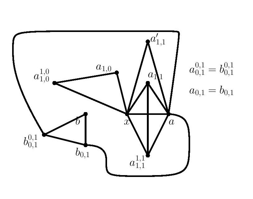
Figure 10.

6.6.1. When $b_{1,1}\in V\left(H^{\prime}_{0}\right)\setminus V(H_{0})$:

When $v_{3}$ is old, we add $\{v_{3},a_{1,0}\}$; when $v_{4}$ is old, we add $\{v_{4},b_{0,1}\}$; when $v_{2}$ is old, we add $\{v_{2},b\}$ and $\{v_{2},b_{1,1}\}$. If $v_{1}=a$, we add edge $\{a,b\}$, which can coincide with $\{v_{2},b\}$ only if $v_{2}=a$. If $v_{1}\in S_{1}\setminus\{a,b_{1,1}\}$, we add edges $\{v_{1},b\}$ and $\{v_{1},b_{0,1}\}$ – even if $v_{1}=v_{2}=v_{4}=v$ for some $v\in S_{2}$, the edges are $\{v,b_{0,1}\}$, $\{v,b\}$, $\{v,b_{1,1}\}$. Any $2$ coinciding banal first-level vertices bring at least $4$ edges; any $3$ bring at least $5$ edges; if all $4$ are banal coincide, they bring $6$ edges. The first-level vertices contribute at least $2\nu_{1}+4$ edges, so that

$$\rho(H_{2})\geq\frac{16+2+(2\nu_{1}+4)+2\nu_{2}+e}{10+1+\nu_{1}+\nu_{2}}=\frac{22+2(\nu_{1}+\nu_{2})+e}{11+(\nu_{1}+\nu_{2})}\geq 2>\frac{13}{7}.$$ (6.28)

6.6.2. When $b_{1,1}=a_{1,1}$:

The only scenario where $2$ old first-level vertices together contribute a single edge is when $v_{2}=v_{1}=a$. Any $2$ coinciding banal first-level vertices bring at least $4$ edges; any $3$ bring at least $5$ edges; if all $4$ are banal coincide, they bring $6$ edges. The first-level vertices contribute at least $2\nu_{1}+3$ edges when $\nu_{1}\leq 2$, and at least $2\nu_{1}+4$ when $\nu_{1}\geq 3$, so that

$$\rho(H_{2})\geq\frac{16+1+2\nu_{1}+3+2\nu_{2}+e}{10+\nu_{1}+\nu_{2}}=\frac{20+2(\nu_{1}+\nu_{2})+e}{10+(\nu_{1}+\nu_{2})}\geq 2>\frac{13}{7}.$$ (6.29)

6.6.3. When $b_{1,1}\in\left\{a_{1,1}^{1,1},a^{\prime}_{1,1}\right\}$:

The analysis of § 6.6.2 applies mutatis mutandis here.

6.6.4. When $b_{1,1}=a_{1,0}$:

Any $2$ old first-level vertices bring at least $2$ edges, any $3$ bring at least $3$ edges, and when all $4$ are old, they bring $3$ edges and no more only if $v_{1}=v_{2}=v_{3}=v_{4}=v$ for some $v\in S_{2}$. Any $2$ coinciding banal first-level vertices bring at least $4$ edges, any $3$ bring at least $5$, and if all $4$ are banal and coincide, the common vertex is adjacent to $x$, $a$, $b$, $b_{0,1}$ and $a_{1,0}$. Thus first-level vertices contribute at least $2\nu_{1}+3$ edges when $\nu_{1}\leq 1$ and at least $2\nu_{1}+4$ edges when $\nu_{1}\geq 2$. The remaining analysis is the same as in § 6.6.2.

6.6.5. When $b_{1,1}=a_{1,0}^{1,0}$:

The first-level vertices contribute at least $2\nu_{1}+4$ edges, so that

$$\rho(H_{2})\geq\frac{16+1+(2\nu_{1}+4)+2\nu_{2}+e}{10+\nu_{1}+\nu_{2}}=\frac{21+2(\nu_{1}+\nu_{2})+e}{10+(\nu_{1}+\nu_{2})}>2>\frac{13}{7}.$$ (6.30)

6.6.6. When $b_{1,1}=a$:

The first-level vertices bring at least $2\nu_{1}+3$ edges, and the analysis is the same as in § 6.6.2.

6.7. Eighth case:

We assume that $a_{0,1}$ is a new vertex and $a_{0,1}^{0,1}=b$, and add edges $\{a,b\}$, $\{a,a_{0,1}\}$ and $\{a_{0,1},b\}$ to get $H_{0}$ in Figure 11 with $17$ edges and $11$ vertices.

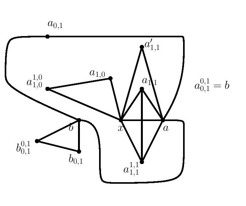
Figure 11.

6.7.1. When $b_{1,1}\in V\left(H^{\prime}_{0}\right)\setminus V(H_{0})$:

When $v_{1}$ is old, it brings $\{v_{1},b_{0,1}\}$; when $v_{2}$ is old, it brings $\{v_{2},b_{1,1}\}$; when $v_{3}$ is old, it brings $\{v_{3},a_{1,0}\}$; when $v_{4}$ is old, it brings $\{v_{4},a_{0,1}\}$. Of these, only $\{v_{3},a_{1,0}\}$ and $\{v_{2},b_{1,1}\}$ may coincide, which happens only if $v_{3}=b_{1,1}$ and $v_{2}=a_{1,0}$, but in that case we additionally get edges $\{a_{1,0},b\}$ and $\{a,b_{1,1}\}$. Any $2$ coinciding banal first-level vertices bring at least $4$ edges, any $3$ at least $5$ edges, and all $4$ bring $7$ edges. The first-level vertices thus contribute at least $2\nu_{1}+4$ edges, so that

$$\rho(H_{2})\geq\frac{17+2+(2\nu_{1}+4)+2\nu_{2}+e}{11+1+\nu_{1}+\nu_{2}}=\frac{23+2(\nu_{1}+\nu_{2})+e}{12+(\nu_{1}+\nu_{2})}\geq\frac{23}{12}>\frac{13}{7}.$$ (6.31)

6.7.2. When $b_{1,1}=a$:

When $v_{1}$ is old, it brings $\{v_{1},b_{0,1}\}$; when $v_{2}$ is old, it brings $\{v_{2},b\}$; when $v_{3}$ is old, it brings $\{v_{3},a_{1,0}\}$; when $v_{4}$ is old, it brings $\{v_{4},a_{0,1}\}$ – all these edges are distinct. Any $2$ coinciding banal first-level vertices bring at least $4$ edges, any $3$ at least $5$ edges, and all $4$ bring $6$ edges. The first-level vertices thus contribute at least $2\nu_{1}+4$ edges, so that

$$\rho(H_{2})\geq\frac{17+(2\nu_{1}+4)+2\nu_{2}+e}{11+\nu_{1}+\nu_{2}}=\frac{21+2(\nu_{1}+\nu_{2})+e}{11+(\nu_{1}+\nu_{2})}\geq\frac{21}{11}>\frac{13}{7}.$$ (6.32)

6.7.3. When $b_{1,1}\in\left\{a_{1,0},a_{1,0}^{1,0}\right\}$:

By the same argument as in § 6.7.2, the first-level vertices bring at least $2\nu_{1}+4$ edges, so that

$$\rho(H_{2})\geq\frac{17+1+(2\nu_{1}+4)+2\nu_{2}+e}{11+\nu_{1}+\nu_{2}}=\frac{22+2(\nu_{1}+\nu_{2})+e}{11+(\nu_{1}+\nu_{2})}\geq 2>\frac{13}{7}.$$ (6.33)

6.7.4. When $b_{1,1}\in S_{2}$:

The first-level vertices contribute at least $2\nu_{1}+3$ edges, so that

$$\rho(H_{2})\geq\frac{17+1+(2\nu_{1}+3)+2\nu_{2}+e}{11+\nu_{1}+\nu_{2}}=\frac{21+2(\nu_{1}+\nu_{2})+e}{11+(\nu_{1}+\nu_{2})}\geq\frac{21}{11}>\frac{13}{7}.$$ (6.34)

6.8. Ninth case:

We assume that $a_{0,1}$ is added as a new vertex and $a_{0,1}^{0,1}=b_{0,1}$, and add edges $\{a_{0,1},a\}$, $\{a_{0,1},b_{0,1}\}$ and $\{a,b_{0,1}\}$, to get $H_{0}$ in Figure 12 with $17$ edges and $11$ vertices.

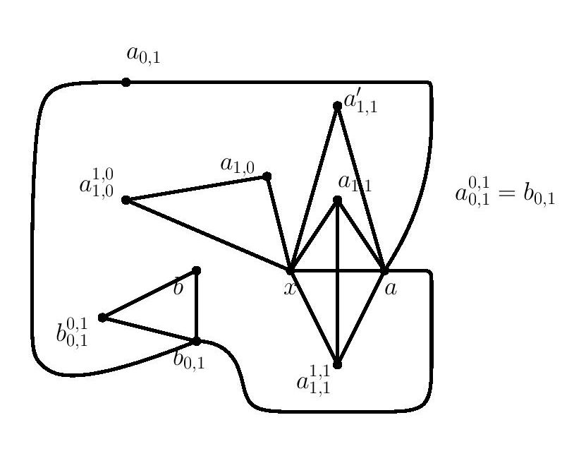
Figure 12.

6.8.1. When $b_{1,1}\in V\left(H^{\prime}_{0}\right)\setminus V(H_{0})$:

When $v_{1}\neq a$ but old, it contributes edge $\{v_{1},b_{0,1}\}$; when $v_{2}$ is old, we get $\{v_{2},b\}$ and $\{v_{2},b_{1,1}\}$; when $v_{3}$ is old, we get $\{v_{3},a_{1,0}\}$; when $v_{4}$ is old, we get $\{v_{4},a_{0,1}\}$ – of these, only $\{v_{3},a_{1,0}\}$ and $\{v_{2},b_{1,1}\}$ may coincide, but this happens only when $v_{2}=a_{1,0}$ and $v_{3}=b_{1,1}$, which brings the additional edge $\{a,b_{1,1}\}$. If $v_{1}=a$, it brings edge $\{a,b\}$, which can coincide with $\{v_{2},b\}$ only when $v_{2}=a$, but in this case we also get the edge $\{a,b_{1,1}\}$ – it either coincides with no other edge added due to old first-level vertices (when $v_{3}\neq b_{1,1}$ and $v_{4}\neq b_{1,1}$), or else we additionally get at least one of the edges $\{b_{1,1},a_{1,0}\}$ (when $v_{3}=b_{1,1}$) and $\{b_{1,1},a_{0,1}\}$ (when $v_{4}=b_{1,1}$). Any $2$ coinciding banal first-level vertices bring at least $4$ edges, any $3$ at least $5$, and all $4$ bring $7$ edges. The first-level vertices thus contribute at least $2\nu_{1}+4$ edges, so that

$$\rho(H_{2})\geq\frac{17+2+(2\nu_{1}+4)+2\nu_{2}+e}{11+1+\nu_{1}+\nu_{2}}=\frac{23+2(\nu_{1}+\nu_{2})+e}{12+(\nu_{1}+\nu_{2})}\geq\frac{23}{12}>\frac{13}{7}.$$ (6.35)

6.8.2. When $b_{1,1}=a_{1,1}$:

The only situation where $2$ old first-level vertices bring a single edge, and no more, is if $v_{1}=v_{2}=a$. When $v_{1}$ is old but $v_{1}\neq a$, it contributes edge $\{v_{1},b_{0,1}\}$, when $v_{2}$ is old, it contributes $\{v_{2},b\}$, when $v_{3}$ is old, it contributes $\{v_{3},a_{1,0}\}$, and when $v_{4}$ is old, it contributes $\{v_{4},a_{0,1}\}$, all of which are distinct. Any $2$ banal, coinciding first-level vertices bring at least $4$ edges, any $3$ bring at least $5$ edges, all $4$ banal and coinciding bring $7$ edges. The first-level vertices bring at least $2\nu_{1}+3$ edges when $\nu_{1}\leq 2$ and at least $2\nu_{1}+4$ edges when $\nu_{1}\geq 3$, so that

$$\rho(H_{2})\geq\frac{17+1+(2\nu_{1}+3)+2\nu_{2}+e}{11+\nu_{1}+\nu_{2}}=\frac{21+2(\nu_{1}+\nu_{2})+e}{11+(\nu_{1}+\nu_{2})}\geq\frac{21}{11}>\frac{13}{7}.$$ (6.36)

6.8.3. When $b_{1,1}\in\left\{a,a_{1,1}^{1,1},a^{\prime}_{1,1}\right\}$:

The analysis of § 6.8.2 applies mutatis mutandis here.

6.8.4. When $b_{1,1}\in\left\{a_{1,0},a_{1,0}^{1,0}\right\}$:

The first-level vertices contribute at least $2\nu_{1}+4$ edges, so that

$$\rho(H_{2})\geq\frac{17+1+(2\nu_{1}+4)+2\nu_{2}+e}{11+\nu_{1}+\nu_{2}}=\frac{22+2(\nu_{1}+\nu_{2})+e}{11+(\nu_{1}+\nu_{2})}\geq 2>\frac{13}{7}.$$ (6.37)

6.9. Tenth case:

We assume that $a_{0,1}$ is added as a new vertex and $a_{0,1}^{0,1}=b_{0,1}^{0,1}$, and add edges $\left\{b_{0,1}^{0,1},a\right\}$, $\left\{b_{0,1}^{0,1},a_{0,1}\right\}$ and $\{a_{0,1},a\}$ to get $H_{0}$ in Figure 13 with $17$ edges and $11$ vertices.

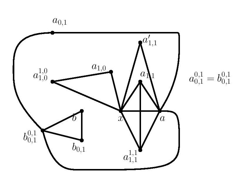
Figure 13.

When $v_{1}$ is old, it brings at least edge $\{v_{1},b_{0,1}\}$, when $v_{2}$ is old, it at least brings edge $\{v_{2},b\}$, when $v_{3}$ is old, it brings $\{v_{3},a_{1,0}\}$, and when $v_{4}$ is old, it brings $\{v_{4},a_{0,1}\}$, all of which are distinct. No matter what $b_{1,1}$ is, any $2$ coinciding banal first-level vertices bring at least $4$ edges, any $3$ bring at least $5$ edges, and all $4$ bring at least $6$ edges. The first-level vertices thus contribute at least $2\nu_{1}+4$ edges, so that when $b_{1,1}\in V\left(H^{\prime}_{0}\right)\setminus V(H_{0})$,

$$\rho(H_{2})\geq\frac{17+2+(2\nu_{1}+4)+2\nu_{2}+e}{11+1+\nu_{1}+\nu_{2}}=\frac{23+2(\nu_{1}+\nu_{2})+e}{12+(\nu_{1}+\nu_{2})}\geq\frac{23}{12}>\frac{13}{7},$$ (6.38)

and when $b_{1,1}\in S_{1}$,

$$\rho(H_{2})\geq\frac{17+1+(2\nu_{1}+4)+2\nu_{2}+e}{11+\nu_{1}+\nu_{2}}=\frac{22+2(\nu_{1}+\nu_{2})+e}{11+(\nu_{1}+\nu_{2})}\geq 2>\frac{13}{7}.$$ (6.39)

6.10. Eleventh case:

We assume that $a_{0,1}=b_{0,1}^{0,1}$ and $a_{0,1}^{0,1}$ is added as a new vertex, and we add edges $\left\{a,b_{0,1}^{0,1}\right\}$, $\left\{a,a_{0,1}^{0,1}\right\}$ and $\left\{a_{0,1}^{0,1},b_{0,1}^{0,1}\right\}$ to get $H_{0}$ in Figure 14 with $17$ edges and $11$ vertices.

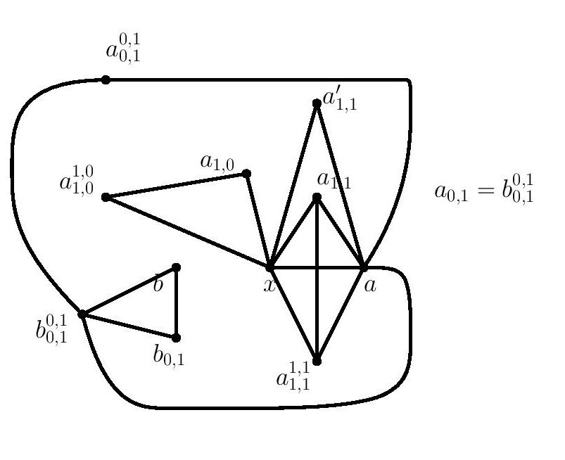
Figure 14.

The argument of § 6.9 applies mutatis mutandis here.

6.11. Twelfth case:

We assume that $a_{0,1}=b_{0,1}^{0,1}$ and $a_{0,1}^{0,1}=b$, and add edges $\left\{a,b_{0,1}^{0,1}\right\}$ and $\left\{a,b\right\}$ to get $H_{0}$ in Figure 15 with $16$ edges and $10$ vertices.

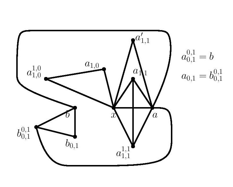
Figure 15.

6.11.1. When $b_{1,1}\in V\left(H^{\prime}_{0}\right)\setminus V(H_{0})$:

When $v_{1}$ ins old, we get $\{v_{1},b_{0,1}\}$; when $v_{4}$ is old, we get $\left\{v_{4},b_{0,1}^{0,1}\right\}$; when $v_{2}$ is old we get $\{v_{2},b_{1,1}\}$; when $v_{3}$ is old, we either get $\{v_{3},a_{1,0}\}$ when $v_{3}\neq b_{1,1}$, or $\{b_{1,1},a_{1,0}\}$ and $\{a,b_{1,1}\}$, only one of which can coincide with $\{v_{2},b_{1,1}\}$. Any $2$ coinciding banal first-level vertices bring at least $4$ edges, any $3$ at least $5$, and all $4$ bring $7$ edges. The first-level vertices thus contribute at least $2\nu_{1}+4$ edges, so that

$$\rho(H_{2})\geq\frac{16+2+(2\nu_{1}+4)+2\nu_{2}+e}{10+1+\nu_{1}+\nu_{2}}=\frac{22+2(\nu_{1}+\nu_{2})+e}{11+(\nu_{1}+\nu_{2})}\geq 2>\frac{13}{7}.$$ (6.40)

6.11.2. When $b_{1,1}=a$:

When $v_{1}$ is old, we get $\{v_{1},b_{0,1}\}$; when $v_{2}$ is old, we get $\{v_{2},b\}$; when $v_{3}$ is old, we get $\{v_{3},a_{1,0}\}$; when $v_{4}$ is old, we get $\left\{v_{4},b_{0,1}^{0,1}\right\}$ – all these edges are distinct. Any $2$ coinciding banal first-level vertices bring at least $4$ edges, any $3$ at least $5$, and all $4$ bring $6$ edges. The first-level vertices thus contribute at least $2\nu_{1}+4$ edges, so that

$$\rho(H_{2})\geq\frac{16+(2\nu_{1}+4)+2\nu_{2}+e}{10+\nu_{1}+\nu_{2}}=\frac{20+2(\nu_{1}+\nu_{2})+e}{10+(\nu_{1}+\nu_{2})}\geq 2>\frac{13}{7}.$$ (6.41)

6.11.3. When $b_{1,1}\in\left\{a_{1,0},a_{1,0}^{1,0}\right\}$:

By the same argument as in § 6.11.2, the first-level vertices contribute at least $2\nu_{1}+4$ edges, so that

$$\rho(H_{2})\geq\frac{16+1+(2\nu_{1}+4)+2\nu_{2}+e}{10+\nu_{1}+\nu_{2}}=\frac{21+2(\nu_{1}+\nu_{2})+e}{10+(\nu_{1}+\nu_{2})}>2>\frac{13}{7}.$$ (6.42)

6.11.4. When $b_{1,1}\in S_{2}$:

The first-level vertices contribute at least $2\nu_{1}+3$ edges, so that

$$\rho(H_{2})\geq\frac{16+1+(2\nu_{1}+3)+2\nu_{2}+e}{10+\nu_{1}+\nu_{2}}=\frac{20+2(\nu_{1}+\nu_{2})+e}{10+(\nu_{1}+\nu_{2})}\geq 2>\frac{13}{7}.$$ (6.43)

6.12. Thirteenth case:

We assume that $a_{0,1}=b_{0,1}^{0,1}$ and $a_{0,1}^{0,1}=b_{0,1}$, and add the edges $\left\{a,b_{0,1}^{0,1}\right\}$ and $\left\{a,b_{0,1}\right\}$ to get $H_{0}$ in Figure 16 with $16$ edges and $10$ vertices.

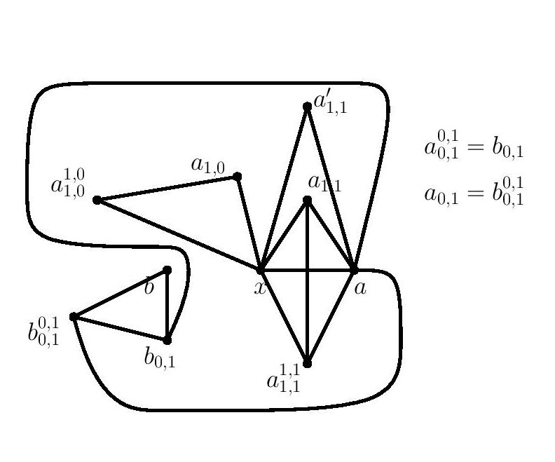
Figure 16.

6.12.1. When $b_{1,1}\in V\left(H^{\prime}_{0}\right)\setminus V(H_{0})$:

When $v_{1}$ is old but $v_{1}\neq a$, we get the edge $\{v_{1},b_{0,1}\}$; when $v_{4}$ is old, we get the edge $\left\{v_{4},b_{0,1}^{0,1}\right\}$; when $v_{3}$ is old, it brings at least the edge $\{v_{3},a_{1,0}\}$; when $v_{2}$ is old, it brings $\{v_{2},b\}$ and $\{v_{2},b_{1,1}\}$. The edges $\{v_{3},a_{1,0}\}$ and $\{v_{2},b_{1,1}\}$ can coincide only if $v_{3}=b_{1,1}$ and $v_{2}=a_{1,0}$, but then we also additionally get $\{a,b_{1,1}\}$. When $v_{1}=a$, we get the edge $\{a,b\}$, which can coincide with $\{v_{2},b\}$ if $v_{2}=a$, but we also get the edge $\{a,b_{1,1}\}$ due to $v_{2}$ which either stays distinct from all other edges added due to old first-level vertices (when $v_{3}\neq b_{1,1}$ and $v_{4}\neq b_{1,1}$), or else is accompanied by at least one of $\{b_{1,1},a_{1,0}\}$ and $\left\{b_{1,1},b_{0,1}^{0,1}\right\}$.

Any $2$ coinciding banal first-level vertices bring at least $4$ edges, any $3$ at least $5$, and all $4$ bring $7$ edges. The first-level vertices thus contribute at least $2\nu_{1}+4$ edges, so that

$$\rho(H_{2})\geq\frac{16+2+(2\nu_{1}+4)+2\nu_{2}+e}{10+1+\nu_{1}+\nu_{2}}=\frac{22+2(\nu_{1}+\nu_{2})+e}{11+(\nu_{1}+\nu_{2})}\geq 2>\frac{13}{7}.$$ (6.44)

6.12.2. When $b_{1,1}\in S_{2}$:

When $v_{3}$ is old, it adds edge $\{v_{3},a_{1,0}\}$; when $v_{4}$ is old, it add edge $\left\{v_{4},b_{0,1}^{0,1}\right\}$ – both these edges are distinct from all other edges added due to old first-level vertices. The only situation where $2$ old first-level vertices together bring a single edge, and no more, is when $v_{1}=v_{2}=a$. Any $2$ coinciding banal first-level vertices bring at least $4$ edges, any $3$ at least $5$, and all $4$ bring $7$ edges. The first-level vertices thus contribute at least $2\nu_{1}+3$ edges when $\nu_{1}\leq 2$ and at least $2\nu_{1}+4$ when $\nu_{1}\geq 3$, so that

$$\rho(H_{2})\geq\frac{16+1+(2\nu_{1}+3)+2\nu_{2}+e}{10+\nu_{1}+\nu_{2}}=\frac{20+2(\nu_{1}+\nu_{2})+e}{10+(\nu_{1}+\nu_{2})}\geq 2>\frac{13}{7}.$$ (6.45)

6.12.3. When $b_{1,1}\in\left\{a_{1,0},a_{1,0}^{1,0}\right\}$:

When $v_{1}$ is old, we get either edge $\{v_{1},b_{0,1}\}$ or $\{a,b\}$; when $v_{2}$ is old, we get $\{v_{2},b\}$ where $v_{2}\neq a$; when $v_{3}$ is old, we get $\{v_{3},a_{1,0}\}$; when $v_{4}$ is old, we get $\left\{v_{4},b_{0,1}^{0,1}\right\}$ – all these edges are distinct. Any $2$ coinciding banal first-level vertices bring at least $4$ edges, any $3$ at least $5$, and all $4$ bring at least $6$ edges. The first-level vertices thus bring at least $2\nu_{1}+4$ edges, so that

$$\rho(H_{2})\geq\frac{16+1+(2\nu_{1}+4)+2\nu_{2}+e}{10+\nu_{1}+\nu_{2}}=\frac{21+2(\nu_{1}+\nu_{2})+e}{10+(\nu_{1}+\nu_{2})}>2>\frac{13}{7}.$$ (6.46)

6.12.4. When $b_{1,1}=a$:

The first-level vertices bring at least $2\nu_{1}+3$ edges, so that

$$\frac{16+1+(2\nu_{1}+3)+2\nu_{2}+e}{10+\nu_{1}+\nu_{2}}=\frac{20+2(\nu_{1}+\nu_{2})+e}{10+(\nu_{1}+\nu_{2})}\geq 2>\frac{13}{7}.$$ (6.47)

References

- [1] Zhukovskii, Maksim, Zero-one k-law, Discrete Mathematics, Volume 312, Issue 10, Pages 1670–1688, 2012, Elsevier.
- [2] Alon, Noga and Spencer, Joel H., The probabilistic method, 2004, John Wiley & Sons.
- [3] Spencer, Joel H., Counting extensions, Journal of Combinatorial Theory, Series A, Volume 55, Issue 2, Pages 247–255, 1990, Elsevier.
- [4] Shelah, Saharon and Spencer, Joel H., Zero–one laws for sparse random graphs, Journal of the American Mathematical Society, Volume 1, Issue 1, Pages 97–115, 1988, JSTOR.
- [5] Spencer, Joel, The strange logic of random graphs, Volume 22, 2013, Springer Science & Business Media.
- [6] Spencer, Joel, Threshold spectra via the Ehrenfeucht game, Discrete Applied Mathematics, Volume 30, Issue 2–3, Pages 235–252, 1991, North-Holland.
- [7] Bollobás, Béla and Wierman, John C., Subgraph counts and containment probabilities of balanced and unbalanced subgraphs in a large random graph, Annals of the New York Academy of Sciences, Volume 576, Issue 1, Pages 63–70, 1989, Wiley Online Library.
- [8] Bollobás, Béla, Threshold functions for small subgraphs, Mathematical Proceedings of the Cambridge Philosophical Society, Volume 90, Issue 2, Pages 197–206, 1981, Cambridge University Press.
- [9] Bollobás, Béla, Random Graphs, Volume 73, 2001, Cambridge University Press.
- [10] Ehrenfeucht, Andrzej, An application of games to the completeness problem for formalized theories, Fund. Math, Volume 49, Issue 13, Pages 129-141, 1961.
- [11] Libkin, Leonid, Elements of finite model theory, 2013, Springer Science & Business Media.
- [12] Immerman, Neil, Descriptive complexity, 2012, Springer Science & Business Media.
- [13] Marker, David, Model Theory, Volume 217, 2006, Springer Science & Business Media.
- [14] Janson, Svante and Luczak, Tomasz and Rucinski, Andrzej, Random graphs, Volume 45, 2011, John Wiley & Sons.
- [15] Kaufmann, Matt, A counterexample to the law for existential monadic second-order logic, CLI Internal Note 32, 1987, Computational Logic Inc.
- [16] Le Bars, Jean-Marie, The 0–1 law fails for monadic existential second-order logic on undirected graphs, Information Processing Letters, Volume 77, Issue 1, Pages 43–48, 2001, Elsevier.
- [17] McArthur, Monica, The asymptotic behavior of on sparse random graphs, Logic and Random Structures, Pages 53–64, 1995.
- [18] Razafimahatratra, AS and Zhukovskii, M, Zero–one laws for -variable first-order logic of sparse random graphs, Discrete Applied Mathematics, Volume 276, Pages 121–128, 2020, Elsevier.