Period integrals from wall structures via tropical cycles, canonical coordinates in mirror symmetry and analyticity of toric degenerations

Abstract.

We give a simple expression for the integral of the canonical holomorphic volume form in degenerating families of varieties constructed from wall structures and with central fiber a union of toric varieties. The cycles to integrate over are constructed from tropical 1-cycles in the intersection complex of the central fiber.

One application is a proof that the mirror map for the canonical formal families of Calabi-Yau varieties constructed by Gross and the second author is trivial. We also show that these families are the completion of an analytic family, without reparametrization, and that they are formally versal as deformations of logarithmic schemes. Other applications include canonical one-parameter type III degenerations of K3 surfaces with prescribed Picard groups.

As a technical result of independent interest we develop a theory of period integrals with logarithmic poles on finite order deformations of normal crossing analytic spaces.

1. Introduction

A period of a complex manifold $X$ is the integral $\int_{\beta}\alpha$ of a holomorphic differential $k$-form $\alpha$ over a singular $k$-cycle $\beta$ on $X$. The classical example is the elliptic integral $\int dx/\sqrt{x^{3}+ax+b}$, an integral over a closed curve of the holomorphic one form $y^{-1}dx$ on the elliptic curve $y^{2}=x^{3}+ax+b$. More modern accounts emphasize the interpretation of periods in terms of Hodge theory and their dependence on varying $X$ and $\alpha$ in a holomorphic family [Gt70]. This interpretation is of fundamental importance in the study of moduli spaces [CMSP]. Another fascinating aspect of period integrals is the countable set of values obtained for algebraic varieties defined over $\mathbb{Q}$ [KZ].

The main result of this paper gives a simple closed formula of a class of period integrals for families of complex manifolds naturally arising in mirror symmetry and in the study of cluster varieties. The families $\mathcal{X}\to S$ considered have a special fiber $X_{0}$ that is a union of projective toric varieties of dimension $n$, glued pairwise along toric divisors. In particular, $X_{0}$ is normal crossings outside a subset of codimension two. The special fiber is conveniently represented by the union of momentum polytopes, glued pairwise along their facets according to the gluing of the irreducible components of $X_{0}$, thus forming a cell complex $\mathscr{P}$ with underlying topological space $B$ a pseudo-manifold, possibly with boundary. Outside codimension two, the family $\mathcal{X}\to S$ is built from toric pieces via special isomorphisms encoded in a wall structure on $B$. The special isomorphisms respect the toric holomorphic differential $n$-forms $z_{1}^{-1}dz_{1}\wedge\ldots\wedge z_{n}^{-1}dz_{n}$, which thus define a global relative holomorphic $n$-form $\Omega$ for $\mathcal{X}$ over the parameter space $S$.

For example, for any Laurent polynomial $f\in\mathbb{C}[u_{1}^{\pm 1},\ldots,u_{n-1}^{\pm 1}]$, the family of subvarieties

(1.1) $$zw=f\cdot t^{\kappa}$$

of $\mathbb{C}^{2}\times(\mathbb{C}^{*})^{n-1}$ parametrized by $t\in\mathbb{C}$ is of this form. Such families arise as mirrors to local Calabi-Yau manifolds [CKYZ],[GS14], and in mirror symmetry for varieties of general type [GKR],[AAK]. If the wall structure is not locally finite, this picture is accurate only at finite orders in the deformation parameter. A careful treatment of period integrals with logarithmic poles at $t=0$ in this setup is given in Appendix A.

In the simplest versions [GS06],[GS11a], $S$ is the spectrum of a discrete valuation ring, or a disk analytically, but in any case, $S$ is an open subset of an affine toric variety or its completion along a toric divisor [GHK],[GHS]. Thus there is a well-defined notion of monomial function on $S$.

For the domain of integration, we consider continuous deformations $\beta_{t}$ of a class of $n$-cycles $\beta$ on $X_{0}$ that generically fiber as a real $(n-1)$-torus bundle over a graph in $B$ and which intersect the singular locus of $X_{0}$ transversely in some sense. In a nutshell, our main result says that in the best cases, which include [GS11a] and [GHK], there are constants $c\in\mathbb{C}$ and a monomial $t^{q}$ on $S$ with

$$\frac{1}{(2\pi\sqrt{-1})^{n-1}}\int_{\beta_{t}}\Omega_{X_{t}}=c+\log t^{q},$$

as a holomorphic function outside $t^{q}=0$ and up to multiples of $2\pi\sqrt{-1}$. This result is highly remarkable since for algebraically parametrized families, period integrals of this form typically lead to transcendental functions. In fact, replacing $t$ by $h\cdot t$ for some invertible analytic function $h$ changes the right-hand side by a summand $\log h$. Thus while the logarithmic monomial behavior can be expected for cycles of our form, the fact that $c$ is a constant is very special to the particular construction of the family $\mathcal{X}\to S$ via a wall structure.

The most obvious application of this result is to mirror symmetry. On the complex side of mirror symmetry, one is looking at families $\mathcal{X}\to S$ of Calabi-Yau varieties with topological monodromy around the critical locus unipotent of maximally possible exponent [CdGP], [De], [Mr93]. In this situation, the limiting mixed Hodge structure on the cohomology of a nearby smooth fiber turns out to be of Hodge-Tate type [De], and exponentials of the kind of period integrals studied here provide a distinguished set of holomorphic functions on the parameter space. These functions provide a set of coordinates at points where the family is semi-universal, that is, where the Kodaira-Spencer map is an isomorphism. Since these functions only depend on discrete choices, they are known as canonical coordinates in mirror symmetry. The identification of the complexified Kähler moduli space of the mirror with complex moduli works by canonical coordinates. Thus our result says that the mirror map is monomial on the subspace generated by our cycles. In favorable situations one obtains full-dimensional pieces of the complexified Kähler cone on the mirror side.

As another important application, we prove a strong analyticity result for the canonical toric degenerations of [GS11a] and their universal refinement in [GHS], Theorem A.7. This result should be important for the symplectic study of canonical toric degenerations.

1.1. Toric degenerations from wall structures

For more precise statements we now give more details on the setup and construction. We work in the general setting of [GHS] and fix a finitely generated $\mathbb{C}$-algebra $A$ and some $k\in\mathbb{N}$. The algebra $A$ provides moduli for the construction and may be assumed to be $\mathbb{C}$ at first reading. The base ring of our degeneration is $A_{k}=A[t]/(t^{k+1})$, so $k$ determines the order of deformation to be considered.

1.1.1. Polyhedral affine manifolds $(B,\mathscr{P})$

The basic arena of all constructions is a cell complex $\mathscr{P}$ of integral polyhedra with underlying topological space $B$ an $n$-dimensional pseudo-manifold with possibly empty boundary ([GHS], Definition 1.1). All constructions happen away from codimension two. We reserve the letter $\sigma$ for maximal cells and $\rho$ for codimension one cells of $\mathscr{P}$, respectively, possibly adorned. For a cell $\tau\in\mathscr{P}$ we denote by $\Lambda_{\tau}\simeq\mathbb{Z}^{\dim\tau}$ the group of integral tangent vector fields on the interior $\operatorname{Int}\tau$ of $\tau$. We also need maximal cells of the barycentric subdivision of a codimension one cell $\rho$, and these are denoted $\underline{\rho}$. By writing $\underline{\rho}$ it is understood that $\rho$ is the codimension one cell of $\mathscr{P}$ containing $\underline{\rho}$.

Denote by $\Delta\subset B$ the union of all $(n-2)$-cells of the barycentric subdivision that lie in the $(n-1)$-skeleton of $\mathscr{P}$, that is, which are disjoint from the interiors of maximal cells. On $B\setminus\Delta$ we assume given an integral affine structure that restricts to the usual integral affine structure on the interiors of maximal cells. Note that this amounts merely to specifying, for each $\underline{\rho}$ not contained in $\partial B$, the parallel transport through $\underline{\rho}$ of a primitive integral vector complementary to $\Lambda_{\rho}$ on one of the two neighboring maximal cells $\sigma$ of $\rho$ to the other neighboring cell $\sigma^{\prime}$. The polyhedral complex $\mathscr{P}$ along with the affine structure on $B=|\mathscr{P}|$ away from $\Delta$ is what we call a polyhedral affine pseudo-manifold. We use the notation $\Delta_{2}\subset\Delta$ for the smaller set defined by the $(n-2)$-skeleton of $\mathscr{P}$.

1.1.2. Kinks $\kappa_{\underline{\rho}}$ and multivalued piecewise affine function $\varphi$

The second piece of data is the collection of exponents $\kappa\in\mathbb{N}\setminus\{0\}$ appearing in the local models (1.1) in codimension one. There is one such exponent for each $\underline{\rho}$, so these exponents may vary along a codimension one cell $\rho$. As a matter of notation, we denote the collection of all $\kappa_{\underline{\rho}}$ by the associated multivalued piecewise affine function $\varphi$ ([GHS], Definition 1.8).

1.1.3. Wall structures

The third piece of data is a wall structure $\mathscr{S}$ on our polyhedral affine pseudo-manifold, as defined in [GHS], Definition 1.22. The wall structure consists of a finite collection of walls, each wall being an $(n-1)$-dimensional rational polyhedron $\mathfrak{p}$ contained in some cell of $\mathscr{P}$, along with an algebraic function $f_{\mathfrak{p}}$. The walls define an $(n-1)$-dimensional cell complex, assumed to cover all $(n-1)$-cells $\rho\in\mathscr{P}$ and to subdivide each maximal cell of $\mathscr{P}$ into (closed) convex chambers, denoted $\mathfrak{u}$. There are thus two kinds of walls, depending on whether the minimal cell of $\mathscr{P}$ containing $\mathfrak{p}$ is a maximal cell $\sigma$ or a codimension one cell $\rho$. In the first case, walls of codimension zero, $f_{\mathfrak{p}}$ is of the form

$$f_{\mathfrak{p}}=1+az^{m}t^{\ell},$$

with $a\in A$, $\ell>0$ and $z^{m}$ the monomial in the Laurent polynomial ring $\mathbb{C}[\Lambda_{\sigma}]\simeq\mathbb{C}[z_{1}^{\pm 1},\ldots,z_{n}^{\pm 1}]$ defined by some $m\in\Lambda_{\sigma}$ tangent to $\mathfrak{p}$. The second case, walls of codimension one, cover the sources of the inductive construction of the wall structure. Such a wall is therefore also called slab and written with a different symbol $\mathfrak{b}$ instead of $\mathfrak{p}$ for easier distinction. In this case, there are no conditions on $f_{\mathfrak{b}}$ other than that the exponents of monomials be tangent to $\rho$, that is,

$$f_{\mathfrak{b}}\in A[\Lambda_{\rho}][t].$$

Here $\Lambda_{\rho}\simeq\mathbb{Z}^{n-1}$ denotes the group of integral tangent vector fields on $\rho$.

1.1.4. Construction of the scheme $X^{\circ}_{k}/A_{k}$

From the wall structure we build a scheme $X_{k}^{\circ}$ over $A_{k}=A[t]/(t^{k+1})$ assuming a consistency condition, by taking one copy $\operatorname{Spec}R_{\mathfrak{u}}$ with $R_{\mathfrak{u}}=A_{k}[\Lambda_{\sigma}]$ for each chamber $\mathfrak{u}\subseteq\sigma$ and one copy of $\operatorname{Spec}R_{\mathfrak{b}}$ with

(1.2) $$R_{\mathfrak{b}}=A_{k}[\Lambda_{\rho}][Z_{+},Z_{-}]/(Z_{+}Z_{-}-f_{\mathfrak{b}}t^{\kappa_{\underline{\rho}}})$$

for each slab $\mathfrak{b}$. A wall $\mathfrak{p}$ of codimension zero defines a wall crossing automorphism of $A_{k}[\Lambda_{\sigma}]$, for $\sigma$ the maximal cell containing $\mathfrak{p}$, see (3.12) below and [GHS], §2.3. The consistency condition in codimension zero ([GHS], Definition 2.13) is equivalent to saying that sequences of such automorphisms identify all $\operatorname{Spec}R_{\mathfrak{u}}$ for chambers contained in the same maximal cell $\sigma$ in a consistent fashion.

If a slab $\mathfrak{b}\subseteq\underline{\rho}$ is a facet of a chamber $\mathfrak{u}\subseteq\sigma$, there is an open embedding

(1.3) $$\operatorname{Spec}R_{\mathfrak{u}}\longrightarrow\operatorname{Spec}R_{\mathfrak{b}}$$

defined by the inclusion $\Lambda_{\rho}\subset\Lambda_{\sigma}$ and by identifying $Z_{+}$ with $z^{\zeta}$ for $\zeta\in\Lambda_{\sigma}$ a generator of $\Lambda_{\sigma}/\Lambda_{\rho}$ pointing from $\rho$ into $\sigma$. For the other chamber $\mathfrak{u}^{\prime}$ containing $\mathfrak{b}$, contained in the maximal cell $\sigma^{\prime}$ with $\sigma\cap\sigma^{\prime}=\rho$, the corresponding homomorphism $R_{\mathfrak{b}}\to R_{\mathfrak{u}^{\prime}}$ maps $Z_{-}$ to $z^{\zeta^{\prime}}$ with $\zeta^{\prime}$ the parallel transport of $-\zeta$ through $\underline{\rho}$. In this procedure there is a choice of co-orientation of $\rho$ that determines which maximal cell to take for $\sigma$, and a choice of $\zeta\in\Lambda_{\sigma}$, but any two choices lead to isomorphic results. Consistency in codimension one provides the necessary cocycle condition to assure the existence of a scheme $X_{k}^{\circ}$ with open embeddings of all $\operatorname{Spec}R_{\mathfrak{u}}$ and $\operatorname{Spec}R_{\mathfrak{b}}$ compatible with all wall crossing automorphisms and all open embeddings (1.3).

If $\partial B\neq\emptyset$, the codimension one cells $\underline{\rho}$ contained in $\partial B$ require a slightly different treatment that turns $\partial B$ into a divisor in $X_{k}^{\circ}$. We do not review this construction here because all our arguments take place on the complement of $\partial B$.

1.1.5. Codimension two locus, partial completion and theta functions

The fiber $X_{0}^{\circ}$ of $X_{k}^{\circ}$ over $t=0$ is a product of $\operatorname{Spec}A$ with a union of toric varieties, one for each maximal cell $\sigma$, glued pairwise canonically along toric divisors as prescribed by the combinatorics of $\mathscr{P}$. By construction, the toric varieties do not contain any toric strata of codimension larger than one. For a maximal cell $\sigma$, the fan of the corresponding toric variety is the $1$-skeleton of the normal fan of $\sigma$, so consists only of the origin and the rays. While it is always possible to add the codimension two strata to $X_{0}^{\circ}$ to arrive at a scheme $X_{0}$, the extension $X_{k}$ of the flat deformation $X^{\circ}_{k}$ of $X_{0}^{\circ}$ to $X_{0}$ is a lot more subtle and in particular, requires a consistency condition in codimension two. The approach taken in [GHK] and [GHS] to produce $X_{k}$ is to rely on the construction of a canonical $A_{k}$-module basis of the homogeneous coordinate ring, consisting of (generalized) theta functions. For $B=(S^{1})^{n}$ these functions indeed agree with Riemannian theta functions. Theta functions will only be used once in this paper, for the construction of the degenerate momentum map in Proposition 2.1. There is one generalized theta function $\vartheta_{m}$ for each integral point $m$ of $B$. We refer to [GHS] for details. Our periods are computed entirely on $X_{k}^{\circ}$ and hence the extension from $X_{k}^{\circ}$ to $X_{k}$ is largely irrelevant here.

1.1.6. Gluing data

One obvious way to introduce parameters in the construction is to compose the open embeddings $\operatorname{Spec}R_{\mathfrak{u}}\to\operatorname{Spec}R_{\mathfrak{b}}$ from (1.3) with an $A_{k}$-linear toric automorphism of $\operatorname{Spec}R_{\mathfrak{u}}$. For $R_{\mathfrak{u}}=A_{k}[\Lambda_{\sigma}]$ such an automorphism is given by a homomorphism $\Lambda_{\sigma}\to A^{\times}$. The choices $s_{\sigma\underline{\rho}}\in\operatorname{Hom}(\Lambda_{\sigma},A^{\times})$ for each $\underline{\rho},\sigma$ with $\underline{\rho}\subset\sigma$ is called (open) gluing data. All previous notions generalize, with consistency in codimension one and two now checked with the open embeddings (1.3) twisted by the given gluing data. Gluing data may spoil projectivity or even the existence of the completed central fiber $X_{0}\supset X_{0}^{\circ}$. Since the details of this extension are not relevant for the present paper, we refer the interested reader to [GHS], Section 5. Gluing data change the period integral and will play an important role in the application to analyticity, hence have to be taken into consideration.

For simplicity of notation we write $X_{0}$ and $X_{k}$ instead of $X_{0}^{\circ}$ and $X_{k}^{\circ}$ in the following discussion, but work only away from strata of codimension larger than one.

1.2. Singular cycles on $X_{0}$ from tropical $1$-cycles

The $n$-cycles considered are defined from $n$-cycles $\beta$ on $X_{0}$ that generically fiber as a finite union of real $(n-1)$-torus bundles over a graph $\beta_{\operatorname{trop}}$ in $B$. The torus fiber over a non-vertex point of $\beta_{\operatorname{trop}}$ in the interior of a maximal cell $\sigma\in\mathscr{P}$ is an orbit under the conormal torus $\xi^{\perp}\otimes U(1)\simeq U(1)^{n-1}$ inside the real torus $\operatorname{Hom}(\Lambda_{\sigma},\mathbb{Z})\otimes_{\mathbb{Z}}U(1)\simeq U(1)^{n}$ acting on the toric irreducible component $X_{\sigma}\subseteq X_{0}$ defined by $\sigma$. The matching of the various orbits at a vertex amounts to the local vanishing of the boundary of $\beta_{\operatorname{trop}}$ as a singular $1$-cycle with twisted coefficients in the local system $\Lambda$.

1.2.1. The degenerate momentum map $\mu:X_{0}\to B$

To globalize we observe that each maximal cell $\sigma$ comes with a momentum map $\mu_{\sigma}:X_{\sigma}\to\sigma$ of the corresponding irreducible component $X_{\sigma}\subseteq X_{0}$. For trivial gluing data (all $s_{\sigma\underline{\rho}}=1$), the $\mu_{\sigma}$ agree on codimension one strata to define a degenerate momentum map $\mu:X_{0}\to B$. This map should be viewed as a limiting SYZ-fibration [SYZ]. There is a partial collapse of torus fibers over the deeper strata of $X_{0}$ described explicitly by the Kato-Nakayama space of $X_{0}$ as a log space, see [AS] for some details. For non-trivial gluing data, the $\mu_{\sigma}$ have to be composed with diffeomorphisms of the maximal cells $\sigma$ to make them match over common strata. In the projective setting one can use generalized theta functions for a canonical construction, otherwise there may be obstructions to the existence of $\mu$ in codimension two. The following is Proposition 2.1.

Proposition 1.1.

If $X_{0}$ is projective, there exists a degenerate momentum map $\mu:X_{0}\to B$. Without the projectivity assumption, such a map exists at least on the complement of the union of toric strata of $X_{0}$ of codimension two.

1.2.2. The log singular locus $Z\subset X_{0}$, its amoeba image $\mathcal{A}\subset B$ and the adapted affine structure on $B\setminus(\Delta_{2}\cup\mathcal{A})$

For each codimension one cell $\rho\in\mathscr{P}$ and any slab $\mathfrak{b}\subset\rho$, the closure of the zero locus of $f_{\mathfrak{b}}$ defines a hypersurface $Z_{\rho}$ in the codimension one locus $X_{\rho}\subset X_{0}$. By consistency, this zero locus is independent of the chosen slab on $\rho$. From the local equation in codimension one (1.1),(1.2), it follows that $Z_{\rho}$ is the locus where the degeneration is not semi-stable and is indeed singular even from the logarithmic point of view. We define the log singular locus,

$$Z=\bigcup_{\rho}Z_{\rho},$$

a codimension two subset of $X_{0}$ lying in the singular locus of $X_{0}$. The image of $Z$ under our degenerate momentum map,

$$\mathcal{A}=\mu(Z),$$

is called its amoeba image. In fact, for each codimension one cell, $\mathcal{A}\cap\operatorname{Int}\rho$ is a diffeomorphic image of the hypersurface amoeba of $f_{\mathfrak{b}}$, for any slab $\mathfrak{b}\subset\rho$. If the base ring $A$ is higher dimensional, we first take a base change $A\to\mathbb{C}$ to restrict to a slice of the deformation $X_{k}\to\operatorname{Spec}A_{k}$ or work with a small analytic subset of $\operatorname{Spec}A$ for otherwise $\mathcal{A}$ may be too large to be useful.

For $x\in B\setminus(\Delta_{2}\cup\mathcal{A})$ and $\mathfrak{b}$ a slab containing $x$, the restriction of $f_{\mathfrak{b}}$ to $\mu^{-1}(x)$ has no zeros. Thus there exists a unique $m_{x}\in\Lambda_{\rho}$ with the restriction of $z^{-m_{x}}f_{\mathfrak{b}}:\mu^{-1}(x)\to\mathbb{C}^{*}$ contractible. This means that the adapted local equation

(1.4) $$Z_{+}\big{(}z^{-m_{x}}Z_{-}\big{)}=\big{(}z^{-m_{x}}f_{\mathfrak{b}}\big{)}t^{\kappa_{\underline{\rho}}}$$

locally analytically describes the toric normal crossings degeneration

$$zw=t^{\kappa_{\underline{\rho}}}$$

by taking $z=Z_{+}$, $w=Z_{-}/f_{\mathfrak{b}}$. This observation motivates the definition of an adapted integral affine structure on $B\setminus(\Delta_{2}\cup\mathcal{A})$ that defines the parallel transport of $-\zeta^{\prime}\in\Lambda_{\sigma^{\prime}}$ through $x$ to be $\zeta-m_{x}$ instead of $\zeta$, the integral tangent vector chosen in connection with the gluing (1.3).

The set of integral tangent vectors for the adapted affine structure now defines a local system $\Lambda$ on $B\setminus(\Delta_{2}\cup\mathcal{A})$ of free abelian groups of rank $n$. The dual local system $\mathcal{H}\!\text{{om}}(\Lambda,\underline{\mathbb{Z}})$ is denoted $\check{\Lambda}$. Note that if $x\in B\setminus(\Delta_{2}\cup\mathcal{A})$ lies in a maximal cell $\sigma$, we have a canonical isomorphism of the stalk $\Lambda_{x}$ with $\Lambda_{\sigma}$.

1.2.3. Tropical $1$-cycles

With the adapted affine structure on $B\setminus(\Delta_{2}\cup\mathcal{A})$ we are now in a position to define the affine geometric data representing our singular $n$-cycles on $X_{0}$.

Definition 1.2.

A tropical one-cycle $\beta_{\operatorname{trop}}$ is a twisted singular one-cycle on $B\setminus(\Delta_{2}\cup\mathcal{A})$ with coefficients in the sheaf of integral tangent vectors $\Lambda$, that is, $\beta_{\operatorname{trop}}\in Z_{1}(B\setminus(\Delta_{2}\cup\mathcal{A}),\Lambda)$.

Thus a tropical one cycle is an oriented graph $\Gamma$ together with a map $h:\Gamma\to B\setminus(\Delta_{2}\cup\mathcal{A})$ and for each edge $e\subseteq\Gamma$ a section $\xi_{e}$ of $(h|_{e})^{*}\Lambda$ such that for each vertex $v$ the cycle condition $\sum_{e\ni v}\pm\xi_{e}=0$ holds, with sign depending on $e$ being oriented toward or away from $v$. We typically assume without restriction that $\xi_{e}\neq 0$ for all $e$. One way to obtain such cycles is from a tropical curve with a chosen orientation on each edge; the tangent vector for an edge $e$ is then given by the oriented integral generator of the tangent space of $e$ multiplied by the weight of the edge. The balancing (cocycle) condition for tropical curves implies that the associated twisted singular chain is a cycle. We may thus think of twisted singular cycles carrying integral tangent vectors as flabby versions of tropical curves. This motivates the use of the word “tropical”.

1.2.4. The singular cycle $\beta$ associated to a tropical $1$-cycle $\beta_{\operatorname{trop}}$

Fix a parameter value $a\in\operatorname{Spec}(A)_{\mathrm{an}}$ and let $X_{0}(a)$ be the fiber of $X_{0}$ over $a$. Let us now assume for simplicity that $\beta_{\operatorname{trop}}$ is transverse to the $(n-1)$-skeleton of $\mathscr{P}$ and that each of its edges $e$ is embedded into a single maximal cell $\sigma$. For each edge $e$, choose a section $S_{e}\subset X_{\sigma}$ of $\mu_{\sigma}:X_{\sigma}\to\sigma$ over $e$, chosen compatibly over vertices. Then define a chain $\beta_{e}$ over $e$ as the orbit of $S_{e}$ under the subgroup of $\operatorname{Hom}(\Lambda_{\sigma},U(1))\simeq U(1)^{n}$ mapping $\xi_{e}$ to $1$. If $\xi_{e}$ is primitive, this subgroup equals $\xi^{\perp}\otimes U(1)\simeq U(1)^{n-1}$, otherwise it is the product of this $(n-1)$-torus with $\mathbb{Z}/m_{e}\mathbb{Z}$ for $m_{e}\in\mathbb{N}\setminus\{0\}$ the index of divisibility of $\xi_{e}$. At a vertex $v$ of $\beta_{\operatorname{trop}}$ the cycle condition $\sum_{e\ni v}\pm\xi_{e}=0$, with signs adjusting for the orientation of the edges at $v$, implies that the boundaries over $v$ of the chains $\beta_{e}$ bound an $n$-chain $\Gamma_{v}$ over $v$. The singular $n$-cycle associated to $\beta_{\operatorname{trop}}$ is now defined as

$$\beta=\sum_{e}\beta_{e}+\sum_{v}\Gamma_{v}.$$

The section $S_{e}$ is only unique in homology up to adding closed circles in fibers; the orbit of such a circle yields a copy of the fiber class of $\mu_{\sigma}$, which is homologically trivial in $X_{0}(a)$, so we obtain the following.

Lemma 1.3.

The association $\beta_{\operatorname{trop}}\mapsto\beta$ induces a well-defined homomorphism

$$H_{1}(B\setminus(\Delta_{2}\cup\mathcal{A}),\Lambda)\to H_{n}(X_{0}(a),\mathbb{Z}).$$

Remark 1.4.

For $n=2$, the construction of $n$-cycles from tropical one-cycles was done before in [Sy] with a minor variation: Symington’s tropical cycles have boundary in the amoeba image $\mathcal{A}$ of the affine structure, that is, they are relative cycles in $H_{1}(B,\mathcal{A};\iota_{*}\Lambda)$ for $\iota:B\setminus\mathcal{A}\hookrightarrow B$ the inclusion. Note that in this dimension, $\mathcal{A}\subset B$ is a finite set. Symington’s alternative definition gives nothing new compared to our cycles since relative one-cycles with boundary on $\mathcal{A}$ are homologous to cycles with little loops around $\mathcal{A}$ and this process lifts to singular cycles on $X_{0}(a)$. Similar relative cycles in higher dimension are more peculiar; one needs to replace $\iota_{*}\Lambda$ by a subsheaf of $\iota_{*}\Lambda$, see [Ru19] for details.

If $\beta_{\operatorname{trop}}$ is the tropical cycle associated to a tropical curve and the section $S$ the restriction of the positive real locus in a real degeneration situation, as discussed in [AS], then $\beta$ is a Lagrangian cell complex. A related situation for $n=3$ arises in [MR] for $n=3$.

More generally, a similar procedure produces singular cycles in $H_{n-p+q}(X_{0}(a),\mathbb{Z})$ from cycles in $H_{q}(B,\iota_{*}\bigwedge^{p}\Lambda)$, well-defined up to adding cycles constructed from $H_{q-1}(B,\iota_{*}\bigwedge^{p-1}\Lambda)$. For tropical cycles with boundary in $\mathcal{A}$, more care needs to be taken. See [CBM] for an application of relative tropical 2-cycles to conifold transitions, see also [Ru19].

The point of using the adapted affine structure on $B\setminus(\Delta_{2}\cup\mathcal{A})$ is as follows. For any analytic family $\mathcal{X}\to D$ with central fiber $X_{0}(a)$ and given by (1.2) locally in codimension one, there is a continuous family of $n$-cycles $\beta(t)$ for $t\in D\setminus\mathbb{R}_{<0}$ with $\beta(0)=\beta$. The reason for having to remove $\mathbb{R}_{<0}$ in this statement is the topological monodromy action on $\beta(t)$ for varying $t$ in a loop around the origin.

At a vertex $v$ of $\beta_{\operatorname{trop}}$ on a slab $\mathfrak{b}\subseteq\rho$, the local situation is as follows. If $\xi_{e}\in\Lambda_{\rho}$, then, in adapted coordinates, $zw=t^{\kappa_{\underline{\rho}}}$ describes $\mathcal{X}$ locally, and the cycle $\beta$ is locally a product of an $(n-2)$-chain $\gamma\approx U(1)^{n-2}$ with the union of two disks $|z|\leq 1$, $|w|\leq 1$. In this case, $\beta(t)$ equals $\gamma$ times the cylinder $zw=t^{\kappa_{\underline{\rho}}}$, $|z|,|w|\leq 1$ and the local topological monodromy is trivial. Otherwise, $\beta$ is locally the product of an $(n-1)$-chain $\gamma\approx U(1)^{n-1}$ with a curve $\iota$ connecting $z=1,w=0$ with $z=0,w=1$. In deforming to $t\neq 0$ we can again leave $\gamma$ untouched, but the curve $\iota$ deforms to a curve $\iota(t)$ on the cylinder connecting $(z,w)=(1,1/t^{\kappa_{\underline{\rho}}})$ to $(z,w)=(1/t^{\kappa_{\underline{\rho}}},1)$. The topological monodromy acts on $\iota(t)$ by a $\kappa_{\underline{\rho}}$-fold Dehn twist. These Dehn-twists leave an expected ambiguity of the construction of $\beta(t)$ by multiples of the vanishing cycle $\alpha\approx(S^{1})^{n}$. Note that there are also continuous families of cycles homologous to $\alpha$ that converge to a fiber of the degenerate momentum map $\mu$. In particular, $\alpha$ can be interpreted as a fiber of the SYZ fibration. Note also that $\alpha$ can be viewed as constructed from a generator of $H_{0}(B\setminus(\Delta_{2}\cup\mathcal{A}),\iota_{*}\bigwedge^{0}\Lambda)$ in the generalized construction mentioned in Remark 1.4.

1.2.5. Picard-Lefschetz transformation and $c_{1}(\varphi)$

The effect of Picard-Lefschetz transformations on our singular cycles can be written down purely in terms of affine geometry. Since this expression appears in our period integrals, we review it here. The multivalued piecewise affine function $\varphi$ defines a cohomology class in $H^{1}(B\setminus(\Delta_{2}\cup\mathcal{A}),\check{\Lambda})$ denoted $c_{1}(\varphi)$, see [GHS], §1.2. Cap product then defines an integer valued pairing with tropical cycles, that we denote

(1.5) $$\langle c_{1}(\varphi),\beta_{\operatorname{trop}}\rangle\in\mathbb{Z}.$$

Explicitly, this pairing can be computed as follows. Assume without restriction that $\beta_{\operatorname{trop}}$ is transverse to the $(n-1)$-skeleton of $\mathscr{P}$. Then for a vertex $v$ of $\beta_{\operatorname{trop}}$ on a slab $\mathfrak{b}\subseteq\underline{\rho}$, let $e,e^{\prime}$ be the adjacent edges following the orientation of $\beta_{\operatorname{trop}}$. Denoting $\sigma$ the maximal cell containing $e$, let $\check{d}_{e}\in\check{\Lambda}_{\sigma}$ be the primitive generator of $\Lambda_{\rho}^{\perp}$ evaluating positively on tangent vectors pointing from $\rho$ into $\sigma$. Then $v$ contributes the summand $\langle\check{d}_{e},\xi_{e}\rangle\cdot\kappa_{\underline{\rho}}$ to $\langle c_{1}(\varphi),\beta_{\operatorname{trop}}\rangle$, the sum taken over all vertices of $\beta_{\operatorname{trop}}$ on slabs.

The following is Proposition 2.8.

Proposition 1.5.

Let $\beta_{\operatorname{trop}}\in Z_{1}(B\setminus(\Delta_{2}\cup\mathcal{A}),\Lambda)$ be a tropical one-cycle and let $\beta\in H_{n}(X_{0}(a),\mathbb{Z})$ be the associated singular $n$-cycle. Then the Picard-Lefschetz transformation of the deformation $\beta_{t}$ of $\beta$ to an analytic smoothing $X_{t}$ of $X_{0}(a)$ acts by

$$\beta_{t}\longmapsto\beta_{t}+\langle c_{1}(\varphi),\beta_{\operatorname{trop}}\rangle\cdot\alpha.$$

Here $\alpha\in H_{n}(X_{t},\mathbb{Z})$ is the vanishing cycle.

1.3. Statements of main results

We need two more ingredients before being able to state the main theorem.

1.3.1. Pairing $\beta$ with gluing data

Our gluing data $s=(s_{\sigma\underline{\rho}})$ also produces a first cohomology class, this time in $H^{1}(B\setminus(\Delta_{2}\cup\mathcal{A}),\check{\Lambda}\otimes A^{\times})$. Just as $c_{1}(\varphi)$, this cohomology class can be evaluated on tropical cycles via the cap product to obtain an element of $A^{\times}$. We write

(1.6) $$\langle s,\beta_{\operatorname{trop}}\rangle\in A^{\times}$$

for this pairing. In the notation used for $c_{1}(\varphi)$ above, a vertex $v$ of $\beta_{\operatorname{trop}}$ on a slab contained in $\underline{\rho}$ now contributes $\big{(}s_{\sigma^{\prime}\underline{\rho}}/s_{\sigma\underline{\rho}}\big{)}^{\langle\check{d}_{e},\xi_{e}\rangle}$ as a multiplicative factor in the definition of $\langle s,\beta_{\operatorname{trop}}\rangle$.

1.3.2. The complex Ronkin function

For each value of the parameter space $\operatorname{Spec}A$, each slab function $f_{\mathfrak{b}}$ defines a holomorphic function on $\operatorname{Hom}(\Lambda_{\rho},\mathbb{C}^{*})\simeq(\mathbb{C}^{*})^{n-1}$. Such a holomorphic function $f$ has an associated Ronkin function [Ro] on $\mathbb{R}^{n-1}$, defined by

$$N_{f}(x)=\frac{1}{(2\pi\sqrt{-1})^{n-1}}\int_{\operatorname{Log}^{-1}(x)}\frac{\log|f(z_{1},\ldots,z_{n-1})|}{z_{1}\cdots z_{n-1}}dz_{1}\ldots dz_{n-1},$$

with $\operatorname{Log}(z_{1},\ldots,z_{n})=(\log|z_{1}|,\ldots,\log|z_{n}|)$. This function is piecewise affine on the complement of the hypersurface amoebae $\mathcal{A}_{f}=\operatorname{Log}(f=0)$ and otherwise continuous and strictly convex. It plays a fundamental role in the study of amoebas [PR]. The derivative of $N_{f}$ at a point $x\in\mathbb{R}^{n}\setminus\mathcal{A}_{f}$ is the homology class of the restriction of $f$ to $\operatorname{Log}^{-1}(x)$, as a map $U(1)^{n-1}\to\mathbb{C}^{*}$. In particular, $N_{f}$ is locally constant near $x$ if and only if this map is contractible.

Our period integrals involve the complex version of the Ronkin function for our slab functions $f_{\mathfrak{b}}$. Let $x\in\operatorname{Int}\mathfrak{b}$ and $m_{x}\in\Lambda_{\rho}$ be as in the definition of the adapted affine structure above. Taking $z_{1},\ldots,z_{n-1}$ any toric coordinates on $\operatorname{Spec}\mathbb{C}[\Lambda_{\rho}]$, we define the complex Ronkin function of $f_{\mathfrak{b}}$ at $x$ by

(1.7) $$\mathcal{R}(z^{-m_{x}}f_{\mathfrak{b}},x):=\frac{1}{(2\pi\sqrt{-1})^{n-1}}\int_{\mu^{-1}(x)}\frac{\log\big{(}z^{-m_{x}}f_{\mathfrak{b}}(z_{1},\ldots,z_{n-1})\big{)}}{z_{1}\cdots z_{n-1}}dz_{1}\ldots dz_{n-1}\in\mathbb{C}\llbracket t\rrbracket.$$

Under variation of parameters, that is, changing $A\to\mathbb{C}$, the log singular locus $Z$ and in turn the image $\mathcal{A}$ moves. But as long as $x\not\in\mathcal{A}$, the complex Ronkin function varies analytically with the parameters, hence defines a holomorphic function on appropriate open subsets of $\operatorname{Spec}(A)_{\mathrm{an}}$. Note also that the real part of $\mathcal{R}(z^{-m_{x}}f_{\mathfrak{b}},x)$ equals $N_{z^{-m_{x}}f_{\mathfrak{b}}}$. But $z^{-m_{x}}f_{\mathfrak{b}}$ is topologically contractible by the definition of $m_{x}$ and hence $N_{z^{-m_{x}}f_{\mathfrak{b}}}$ is locally constant. In turn, the complex Ronkin function is also locally constant, so does not depend on the choice of $x$ inside a connected component of $\mathfrak{b}\setminus\mathcal{A}$. Reference [PR] contains some more results on the complex Ronkin function, notably a power series expansion in terms of the coefficients of $f_{\mathfrak{b}}$. In general the information captured by the complex Ronkin function does not seem to be well-understood.

Given a tropical cycle $\beta_{\operatorname{trop}}$ as before, we weight the complex Ronkin function at a vertex $v$ of $\beta_{\operatorname{trop}}$ on a slab $\mathfrak{b}$ by $\langle\check{d}_{e},\xi_{e}\rangle\mathcal{R}(z^{-m_{v}}f_{\mathfrak{b}},v)$, notations as above. The sum of all these contributions is denoted

(1.8) $$\mathcal{R}(\beta_{\operatorname{trop}})\in\mathcal{O}(U)\llbracket t\rrbracket,$$

for $U\subset\operatorname{Spec}(A)_{\mathrm{an}}$ an open subset preserving the condition $x\not\in\mathcal{A}$ as discussed.

The complex Ronkin function $\mathcal{R}(z^{-m_{v}}f_{\mathfrak{b}},v)$ is trivial (constant $0$) in one important situation.

Proposition 1.6.

Assume that in a neighborhood of $\mu^{-1}(x)$ there is a convergent infinite product expansion

$$z^{-m_{x}}f_{\mathfrak{b}}=\prod_{i=1}^{\infty}(1+a_{i}z^{m_{i}}t^{\ell_{i}})$$

with $a_{i}\in A$ and all $m_{i}\neq 0$. Then $\mathcal{R}(z^{-m_{x}}f_{\mathfrak{b}},x)=0$.

Proof.

By assumption we have a convergent Laurent expansion of $\log(z^{-m_{x}}f_{\mathfrak{b}})$:

$$\log\big{(}z^{-m_{x}}f_{\mathfrak{b}}\big{)}=\sum_{i}\log\big{(}1+a_{i}z^{m_{i}}t^{\ell_{i}}\big{)}=\sum_{i}\sum_{j>0}\frac{(-1)^{j-1}}{j}a_{i}^{j}z^{jm_{i}}t^{j\ell_{i}}.$$

The integral defining the complex Ronkin function can then be done term-wise. Since $m_{i}\neq 0$ for any $i$, the integral of $z^{jm_{i}}$ over the real torus $\mu^{-1}(x)$ vanishes. ∎

For the slab functions appearing in the wall structures of [GS11a], the criterion of Proposition 1.6 is fulfilled by the so-called normalization condition, see [GS11a], §3.6.

1.3.3. Period integrals

Let us now assume that we have a polyhedral affine manifold $(B,\mathscr{P})$, gluing data $s=(s_{\sigma\underline{\rho}})$ and a wall structure on $B$ consistent in codimension zero and one to order $k$, parametrized by a finitely generated $\mathbb{C}$-algebra $A$. We then obtain $X_{k}^{\circ}$, the flat deformation of $X_{0}^{\circ}$ over $A_{k}=A[t]/(t^{k+1})$ and, for each point $a\in\operatorname{Spec}(A)_{\mathrm{an}}$, the amoeba image $\mathcal{A}=\mu(Z)\subset B$ of the log singular locus $Z$ in the fiber $X_{0}^{\circ}(a)$ of $X_{0}^{\circ}$ over $a$. Let $\Omega$ be the canonical relative holomorphic $n$-form on $X_{k}^{\circ}/A_{k}$ coming with the construction.

Here is the first main result of the paper, proved in §3.6.

Theorem 1.7.

Let $\beta_{\operatorname{trop}}\in Z_{1}(B\setminus(\Delta_{2}\cup\mathcal{A}),\Lambda)$ be a tropical one-cycle and $\beta$ an associated singular $n$-cycle on $X_{0}^{\circ}(a)$. Then using notations introduced in (1.5),(1.6) and (1.8), it holds

(1.9) $$\exp\bigg{(}\frac{1}{(2\pi\sqrt{-1})^{n-1}}\int_{\beta}\Omega\bigg{)}=\exp\big{(}\mathcal{R}(\beta_{\operatorname{trop}})\big{)}\cdot\langle s,\beta_{\operatorname{trop}}\rangle\cdot t^{\langle c_{1}(\varphi),\beta_{\operatorname{trop}}\rangle}.$$

According to Proposition A.5 and Proposition A.6, this result is well-defined up to multiplication with $\exp(h\cdot t^{k+1})$ with $h\in\hat{A}\llbracket t\rrbracket$ for $\hat{A}$ the completion of $A$ at the maximal ideal corresponding to $a$, and it agrees up to such changes with the corresponding analytic integral for any flat analytic family $\mathcal{X}\to U\times\mathbb{D}$ over an analytic open subset $U\times\mathbb{D}\subset\operatorname{Spec}(A[t])_{\mathrm{an}}$ with reduction modulo $t^{k+1}$ equal to $X_{k}^{\circ}$.

In the statement of Theorem 1.7, the ambiguity of $\beta$ from adding multiples of the vanishing cycle $\alpha$ disappears by exponentiation since $\int_{\alpha}\Omega=(2\pi\sqrt{-1})^{n}$ (Lemma 3.1).

In practice one has a mutually compatible system of wall structures $\mathscr{S}_{k}$ consistent to increasing order $k$ and with an increasing, often unbounded number of walls for $k\to\infty$. Theorem 1.7 then gives a formula for the period integral as an element of the quotient field completion $\hat{A}\llbracket t\rrbracket$. In this formula only the complex Ronkin function $\mathcal{R}(\beta_{\operatorname{trop}})$ potentially varies with $k$, capturing higher order corrections to the slab functions $f_{\mathfrak{b}}$ as $k\to\infty$.

Remark 1.8.

A straightforward generalization of Theorem 1.7 deals with base spaces $A\llbracket Q\rrbracket$ for $Q$ a toric monoid as in [GHS]. Then $c_{1}(\varphi)\in H^{1}(B\setminus(\Delta_{2}\cup\mathcal{A}),\check{\Lambda}\otimes Q^{\operatorname{gp}})$ and $f_{\mathfrak{b}}\in A[\Lambda_{\rho}][Q]$. Thus $\langle c_{1}(\varphi),\beta_{\operatorname{trop}}\rangle\in Q^{\operatorname{gp}}$ and the right-hand side of formula 1.9 makes sense as an element of $\hat{A}[Q^{\operatorname{gp}}]$ when writing the monomials of $\mathbb{C}[Q^{\operatorname{gp}}]$ as $t^{q}$ for $q\in Q^{\operatorname{gp}}$. This more general form follows easily from the stated version by testing the statement on a dense set of $\operatorname{Spf}A\llbracket Q\rrbracket$ by base-changing via various morphisms $\operatorname{Spf}\big{(}\hat{A}\llbracket t\rrbracket\big{)}\to\operatorname{Spf}\big{(}\hat{A}\llbracket Q\rrbracket\big{)}$.

A particularly nice situation occurs when $B$ has simple singularities, as introduced in [GS06], Definition 1.60. Morally, these are the singularities that are indecomposable from the affine geometric point of view. In dimension two, simple singularities lead to local models with slab functions with at most one simple zero, that is $zw=(1+\lambda u)\cdot t^{\kappa}$ for some $\lambda\in\mathbb{C}$. In dimension three, the local models are $zw=(1+\mu u_{1}+\nu u_{2})\cdot t^{\kappa}$ or $xyz=(1+\lambda u)\cdot t^{\kappa}$ with $\lambda,\mu,\nu\in\mathbb{C}$. Then the algorithm of [GS11a] produces a canonical formal family $\mathfrak{X}\to\operatorname{Spf}\big{(}A\llbracket t\rrbracket\big{)}$ with central fiber $\operatorname{Spec}A$ classifying log Calabi-Yau spaces over the standard log point with intersection complex $(B,\mathscr{P})$, see [GHS], Theorem A7. Our second main theorem says that locally this family is the completion of an analytic family.

Theorem 1.9 (Theorem 4.4).

Assume that $(B,\mathscr{P})$ has simple singularities, $B$ is orientable and $\partial B$ again an affine manifold with singularities (e.g. empty). Then for each closed point $a\in\operatorname{Spec}A$ there exists an analytic open neighborhood $U$ of $a$ in $\operatorname{Spec}(A)_{\mathrm{an}}$, a disk $\mathbb{D}\subset\mathbb{C}$ and an analytic toric degeneration

$$\mathcal{Y}\longrightarrow U\times\mathbb{D}$$

with completion at $(a,0)$ isomorphic, as a formal scheme over $A\llbracket t\rrbracket$, to the corresponding completion of the canonical toric degeneration $\mathfrak{X}\to\operatorname{Spf}\big{(}A\llbracket t\rrbracket\big{)}$ from [GHS], Theorem A.8.

Moreover, this completion is a hull for the logarithmic divisorial log deformation functor defined in [GS10], Definition 2.7.

The proof occupies Section 4. The hard part of this theorem is that it is not just an approximation result: the isomorphism of the two formal families does not require any change of parameters. Thus the canonical toric degenerations from [GS11a] really are just an algebraic order by order description of an analytic log-versal family with monomial period integrals, that is, written in canonical coordinates.

History of the results. The tropical construction of $n$-cycles and the main period computation in this paper, for the case of [GS11a] with trivial gluing data, has been sketched by the second author in a talk at the conference “Symplectic Geometry and Physics” at ETH Zürich, September 3–7, 2007. Details have been worked out in a first version of the paper in 2014 [RS]. The present paper is an essentially complete rewriting of that version, carefully treating period integrals with logarithmic poles in finite order deformations, giving an intrinsic formulation of all terms in the main period theorem (Theorem 1.7), including a treatment of non-normalized slab functions via the Ronkin function and giving a proof of analyticity and versality of canonical toric degenerations (Theorem 4.4 and §4.3).

1.4. Applications

We apply Theorem 1.7 in several interesting examples.

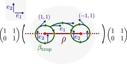
Figure 1.1. A one-dimensional slab $\rho$ with two focus-focus singularities (red) on the left and a two-dimensional slab with amoeba image in red on the right. Tropical one-cycles $\beta_{\operatorname{trop}}$ are given respectively in green and their meeting points with the slabs in orange. Blue arrows on the left give the sections of $\Lambda$ carried by edges of $\beta_{\operatorname{trop}}$.

1.4.1. Mirror dual of $K_{\mathbb{P}^{1}}$

We consider (1.1) alias (1.2) for $f_{\mathfrak{b}}\in\mathbb{C}[u,u^{-1}]$ featuring two zeros as follows

(1.10) $$zw=(au^{-1}+1)(1+bu)t^{\kappa}$$

with $\kappa>0$ and $a,b\in\mathbb{C}^{\times}$, $a\neq b$. The corresponding affine manifold $B$ is shown on the left in Figure 1.1, c.f. Figure 2.2 in [GS14]. The two focus-focus singularities are the images of the zeros of $f_{\mathfrak{b}}$ under the momentum map. Figure 1.1 also shows a tropical one-cycle $\beta_{\operatorname{trop}}$, and Theorem 1.7 yields

(1.11) $$\exp\Big{(}\frac{1}{2\pi\sqrt{-1}}\int_{\beta}\Omega\Big{)}=a\cdot b,$$

for $\beta$ the associated singular $2$-cycle. Indeed, one checks that the contributions in $t$ arising from the two orange points on the same green circle cancel. There are also no contributions from the trivial gluing data. By the product expansion (1.10) and Proposition 1.6, the Ronkin term vanishes at the two inner crossing points where this expansion is valid. However, for the two outer crossings, $f_{\mathfrak{b}}$ is to be multiplied by $z^{-m_{x}}$, which is $u$ and $u^{-1}$, respectively. These crossings produce the constant factors $a$ and $b$ in (1.11).

The geometry here arises as the mirror dual of $K_{\mathbb{P}^{1}}$, a smoothing of the $A_{1}$-singularity. Indeed, $a=b=1$ yields an $A_{1}$-singularity at $x=y=u+1=0$. Our period computes the integral over the vanishing $2$-sphere.

1.4.2. Mirror dual of $K_{\mathbb{P}^{2}}$

We go up one dimension and consider a particular $f_{\mathfrak{b}}\in\mathbb{C}[x^{\pm 1},y^{\pm 1}]$ whose zero-set is an elliptic curve so that (1.1) gives

(1.12) $$zw=(1+x+y+s(xy)^{-1})t^{\kappa}$$

for $s\in\mathbb{C}^{\times}$ a parameter. This geometry arises as the mirror dual of $K_{\mathbb{P}^{2}}$, as studied before in [CKYZ], §2.2 and from a toric degeneration point of view in [GS11b], Example 5.2 and [GS14], Figure 2.1. The corresponding real affine manifold is shown on the right of Figure 1.1 with the amoeba of the elliptic curve the solid red area. The amoeba complement in the slab has one bounded and three unbounded components. The monomial $z^{-m_{p}}$ at a point $p$ inside one of the components equals $1,x^{-1},y^{-1},xy$, respectively. To compute the contribution of the Ronkin function, we write $z^{-m_{p}}\cdot f_{\mathfrak{b}}$ as an infinite product as discussed in [GS14]. Define integers $a_{ijk}$ by the identity

(1.13) $$1+x+y+z=\prod_{i,j,k=0}^{\infty}(1+a_{ijk}x^{i}y^{j}z^{k})$$

and then $h:=\prod_{k=1}^{\infty}(1+a_{kkk}s^{k})$. Inserting $z=s(xy)^{-1}$ in (1.13) now yields a factorization of the slab function $f_{\mathfrak{b}}$ in (1.12) as the product of $h$ and terms fulfilling the hypothesis of Proposition 1.6. Thus the Ronkin term of the period integral at each of the three crossings of the tropical cycle in the bounded center region of the amoeba complement equals $\log(h)$. The Ronkin terms for crossings of the unbounded regions vanish readily by Proposition 1.6, except for the constant term of $xy\cdot f_{\mathfrak{b}}$, which yields $\log(s)$.

Thus, by Theorem 1.7, the exponentiated period integral for the tropical cycle $\beta_{\operatorname{trop}}$ depicted in green in Figure 1.1 yields

(1.14) $$\exp\Big{(}\frac{1}{(2\pi\sqrt{-1})^{2}}\int_{\beta}\Omega\Big{)}=h^{3}\cdot s.$$

The smoothing algorithm of [GS11a] replaces $f_{\mathfrak{b}}$ by $f_{\mathfrak{b}}+g$, where $g=-2s+5s^{2}-32s^{3}+\ldots$ is determined by the normalization condition saying that $\log(f_{\mathfrak{b}}+g)$ has no pure $s$-powers ([GS11a], §3.6). See also [GZ], p.14 and [GS14], Example 3.1,(2). With the normalized slab function $f_{\mathfrak{b}}+g$, the factor $h^{3}$ disappears, leaving only $s$ for the exponentiated period integral (1.14). This illustrates the mechanism relating the normalization condition and the fact that the exponentials of periods for the canonical toric degenerations of [GS11a] are monomials in the base of the family, see also §1.4.5 below. For a related enumerative interpretation of the normalization condition see [CCLT], Theorem 1.6.

1.4.3. Degenerations of K3 surfaces with prescribed Picard group

For a K3 surface $Y$ with holomorphic volume form $\Omega$, an integral homology class $\beta\in H_{2}(Y,\mathbb{Z})$ is the first Chern class of a holomorphic line bundle if and only if its Poincaré-dual class $\hat{\beta}\in H^{2}(Y,\mathbb{C})$ is of type $(1,1)$. Since $\hat{\beta}$ is real, this condition can be detected by the vanishing of $\int_{\beta}\Omega$:

(1.15) $$\int_{\beta}\Omega=\int_{\beta}\overline{\Omega}=\int_{Y}\hat{\beta}\wedge\Omega\stackrel{{\scriptstyle!}}{{=}}0.$$

Combining this observation with Theorem 1.7 and Theorem 1.9, we obtain the following computation of the Picard lattice of general fibers of the canonical toric degenerations of K3 surfaces constructed in [GS11a]. In this case $B$ is a $2$-sphere and the amoeba locus $\mathcal{A}$ consists of at most $24$ points. This number is achieved if all singularities are of focus-focus type, that is, have local affine monodromy conjugate to $\left(\begin{smallmatrix}1&0\\ 1&1\end{smallmatrix}\right)$. This is the case iff all slab functions have simple zeroes with pairwise different absolute values, for example if $(B,\mathscr{P})$ has simple singularities as explained before Theorem 1.9. In any case, we assume that the affine structure on $B$ extends over the vertices of $\mathscr{P}$, so we can disregard $\Delta_{2}$. The result is then expressed in terms of the singular homology group $H_{1}(B,\iota_{*}\Lambda)$ with $\iota:B\setminus\mathcal{A}\to B$ the inclusion. Before stating the result, we make some comments on this homology group and how it relates to the K3 lattice.

First, if a singular $1$-cycle with coefficients in $\iota_{*}\Lambda$ passes through a point of $\mathcal{A}$, then the integral tangent vector carried at this point is invariant under local integral affine monodromy and hence can be perturbed away from $\mathcal{A}$. In other words, push-forward by $\iota$ defines a surjection

(1.16) $$\iota_{*}:H_{1}(B\setminus(\Delta_{2}\cup\mathcal{A}),\Lambda)\longrightarrow H_{1}(B,\iota_{*}\Lambda).$$

Second, for $\mathcal{Y}\to U\times\mathbb{D}$ the analytic family from Theorem 1.9 and $a\in U\subset\operatorname{Spec}(A)_{\mathrm{an}}$, $t\in\mathbb{D}\setminus\{0\}$, let $Y_{t}=Y_{t}(a)$ denote the fiber over $(a,t)$. Our construction of tropical cycles defines a homomorphism

$$H_{1}(B\setminus\mathcal{A},\Lambda)\longrightarrow H_{2}(Y_{t},\mathbb{Z})/\langle\alpha\rangle,\quad\beta_{\operatorname{trop}}\longmapsto\beta,$$

with $\alpha$ the vanishing cycle. This homomorphism is compatible with the respective intersection pairings (cap product), as is the previous homomorphism (1.16). Third, $H_{1}(B\setminus\mathcal{A},\Lambda)$ together with its intersection pairing only depends on the linear part of the monodromy representation, hence can be computed in any model, by the classical uniqueness result for this monodromy representation ([ML], Theorem on p. 225). For one particular model, Symington in [Sy], §11, has given a basis of tropical cycles spanning the even unimodular lattice $-E_{8}^{\oplus 2}\oplus H^{\oplus 2}$ of rank $20$ and signature $(2,18)$, and these also map to a basis of $H_{1}(B,\iota_{*}\Lambda)$ under (1.16) by unimodularity and a rank computation. This lattice is the orthogonal complement of a hyperbolic plane $H$ in the K3 lattice spanned by a fiber and a section of a K3 surface fibered in Lagrangian tori over $B$. In our situation this fiber class is $\alpha_{t}$ and we have identifications of lattices

$$H_{1}(B,\iota_{*}\Lambda)=\big{\{}\beta_{t}\in H_{2}(Y_{t},\mathbb{Z})\,\big{|}\,\beta_{t}\in\alpha_{t}^{\perp}\big{\}}\big{/}\langle\alpha\rangle\simeq-E_{8}^{\oplus 2}\oplus H^{\oplus 2}.$$

Our period integrals now identify the Picard lattice of $H_{2}(Y_{t},\mathbb{Z})$ inside this lattice.

Corollary 1.10.

Let $\pi:\mathcal{Y}\to U\times\mathbb{D}$ be the analytic version from Theorem 1.9 of the canonical degenerating family of K3 surfaces defined by a polyhedral affine structure $(B,\mathscr{P})$ with underlying topological space $S^{2}$ and simple singularities, strictly convex multivalued piecewise affine function $\varphi$ and gluing data $s\in H^{1}(B,\iota_{*}\check{\Lambda}\otimes\mathbb{C}^{*})$. Then the Picard group of a general fiber $Y_{t}$ of $\pi$ is canonically isomorphic to

$$\big{\{}\beta_{\operatorname{trop}}\in H_{1}(B,\iota_{*}\Lambda)\,\big{|}\,\beta_{\operatorname{trop}}\in c_{1}(\varphi)^{\perp},\,\langle s,\beta_{\operatorname{trop}}\rangle=1\big{\}}.$$

Proof.

Theorem 1.7 implies that $\int_{\beta_{t}}\Omega_{Y_{t}}$ can only be constant if $\langle c_{1}(\varphi),\beta_{\operatorname{trop}}\rangle=0$. If this is the case then $\int_{\beta_{t}}\Omega_{Y_{t}}$ extends holomorphically over $t=0$ and thus $\langle s,\beta_{\operatorname{trop}}\rangle=1$ is equivalent to $\int_{\beta_{t}}\Omega_{Y_{t}}\in(2\pi\sqrt{-1})^{n}\mathbb{Z}$. Noting that $\int_{\alpha_{t}}\Omega_{Y_{t}}=(2\pi\sqrt{-1})^{n}$ for $\alpha_{t}\in H_{2}(Y_{t},\mathbb{Z})$ the class of the vanishing cycle from Proposition 1.5, the equality in (1.16) implies that $\beta_{t}$ is the image of the Poincaré-dual of an integral $(1,1)$ class under the quotient map $H_{2}(Y_{t},\mathbb{Z})\to H_{2}(Y_{t},\mathbb{Z})/\langle\alpha_{t}\rangle$. Since $\alpha_{t}$ can be chosen Lagrangian, it can not be Poincaré-dual to the class of a holomorphic line bundle. Hence the image of $\beta_{t}$ in $H_{2}(Y_{t},\mathbb{Z})/\langle\alpha_{t}\rangle$ is enough to determine the Picard lattice. ∎

Thus for trivial gluing data $s=1$, or $s$ of finite order in $H^{1}(B,\iota_{*}\check{\Lambda}\otimes\mathbb{C}^{*})$, the Picard lattice of $Y_{t}$ has next to largest rank $19$. We thus retrieve families studied intensely, see e.g. [Mr84], [Do].

It is also possible to treat the more general families with non-simple singularities from [GHS], §A.4, by treatment as a limit of a situation with focus-focus singularities. Such models lead to one-parameter families with $A_{k}$-singularities. For trivial gluing data, their resolution still provides families of K3 surfaces with Picard rank $19$. Non-simple singularities are necessary for producing families of K3 surfaces with large Picard rank of low degree. Further details will appear in [GHKS].

Related results from a more elementary perspective have been obtained in [Ya].

1.4.4. Degenerations of rational elliptic surfaces

Another application is to toric degenerations of rational elliptic surfaces. In this case, the formula for period integrals in Theorem 1.7 has been used in the thesis of Lisa Bauer to prove a Torelli theorem for toric degenerations of rational elliptic surfaces with simple singularities. We refer to [Ba],§5 for details.

1.4.5. Canonical Coordinates in Mirror Symmetry

A canonical system of holomorphic coordinates on the base $V$ of a maximally unipotent Calabi-Yau degeneration $\mathcal{Y}\to V$ was first proposed in [Mr93], [De] as follows. Let $\mathcal{Y}_{0}$ denote the maximally degenerate fiber, $V\subset\mathbb{C}^{r}$ a small neighborhood of $0$ and $\mathcal{Y}_{t}$ a regular fiber. Assume the discriminant $D=D_{1}+\ldots+D_{s}\subset V$ is the intersection with $V$ of a union of coordinate hyperplanes and let $T_{i}:H_{n}(\mathcal{Y}_{t},\mathbb{Z})\to H_{n}(\mathcal{Y}_{t},\mathbb{Z})$ be the monodromy transformation along a simple loop around $D_{i}$. If $Y_{0}$ is reduced with simple normal crossings then the $T_{i}$ are unipotent, so $N_{i}=-\log(T_{i})$ is well-defined. Set $N=\sum_{i}\lambda_{i}N_{i}$ for any $\lambda_{i}>0$.

The monodromy weight filtration is the unique filtration $W_{0}\subseteq W_{1}\subseteq W_{2}\subseteq\ldots\subseteq W_{2n}$ on $H_{n}(\mathcal{Y}_{t},\mathbb{Q})$ with the properties $N(W_{i})\subseteq W_{i-2}$ and that $N^{k}:\operatorname{Gr}^{W}_{n+k}\to\operatorname{Gr}^{W}_{n-k}$ is an isomorphism for $\operatorname{Gr}^{W}_{i}=W_{i}/W_{i-1}$. Schmid gave a decreasing filtration $F^{\bullet}_{\lim}$ on $H^{n}(\mathcal{Y}_{t},\mathbb{C})$ which combines with the Poincaré dual filtration $\tilde{W}_{i}:=W^{\perp}_{2n-i}$ to give a mixed Hodge structure. The degeneration $\mathcal{Y}\to V$ is maximally unipotent if this mixed Hodge structure is Hodge-Tate. The latter property implies that $W_{2i}=W_{2i+1}$. If $\mathcal{Y}_{t}$ is Calabi-Yau, then $\dim_{\mathbb{Q}}W_{0}=1$ and $\dim_{\mathbb{Q}}W_{2}/W_{0}=\dim H^{1}(\mathcal{Y}_{t},\Theta_{\mathcal{Y}_{t}})$, so at least dimension-wise it makes sense to expect that a set of cycles $\beta_{1},\ldots,\beta_{r}\in H_{n}(\mathcal{Y}_{t},\mathbb{Z})$ that descends to a basis of $W_{2}/W_{0}$ gives rise to a set of coordinates $h_{i}:=\exp(\int_{\beta_{i}}\Omega)$ for $\Omega$ a suitably normalized relative $n$-form of $\mathcal{Y}\to V$. This was proved in [Mr93], [De]. These coordinates are canonical in the sense of being unique up to an integral change of basis of $W_{2}/W_{0}$. The $h_{i}$ also agree with exponentials of flat coordinates for the special geometry on the Calabi-Yau moduli space defined by the Weil-Petersson metric [Ti],[Sr],[Fr].

Motivated from [SYZ], the Leray filtration of the momentum map was found to coincide with the above weight filtration for $n=3$ [Gr98] §4, so generators for $W_{2}/W_{0}$ should be obtained from one-cycles in $B$ with values in $\Lambda$, as also suggested in [KS] §7.4.1. Note however, this can only work if $H_{1}(B,\iota_{*}\Lambda)$ has large enough rank and it is easy to produce examples where this fails. A way to ensure the rank matches is by requiring $B$ to be simple, see [GS10], [Ru19]. In the simple situation, Corollary 4.6 and §4.3 give directly that the exponentiated periods from cycles in $H^{1}(B,\iota_{*}\Lambda)$ provide coordinates on a versal family. At least in the case with simple singularities, it is expected that the image of the homomorphism

(1.17) $$H_{1}(B\setminus(\Delta_{2}\cup\mathcal{A}),\Lambda)\to H_{n}(Y_{t},\mathbb{Q})/\langle\alpha_{t}\rangle$$

generates $W_{2}$. In general, $W_{0}=\operatorname{im}N^{n}$ and

$$W_{2}=\big{(}\operatorname{im}N^{n-2}\cap\operatorname{ker}N\big{)}+\big{(}\operatorname{im}N^{n-1}\cap\operatorname{ker}N^{2}\big{)}.$$

By Proposition 1.5, $\alpha_{t}\in\operatorname{ker}(N)$ and $\beta\in\operatorname{ker}(N^{2})$ for every $\beta$ obtained from a tropical one-cycle. By [GS10], $N$ can be identified with the Lefschetz operator on the mirror. Thus, by the rotation of the Hodge diamond [GS10] and up to identifying the composition $Y_{t}\to Y_{0}\stackrel{{\scriptstyle\mu}}{{\to}}B$ with a compactification of $T^{*}_{B\setminus(\Delta_{2}\cup\mathcal{A})}/\check{\Lambda}\to B\setminus(\Delta_{2}\cup\mathcal{A})$ in the upcoming work [RZ], we find $\alpha_{t}\in\operatorname{im}N^{n}$ and the image of (1.17) indeed generates $W_{2}$. The geometry over $B\setminus(\Delta_{2}\cup\mathcal{A})$ has been investigated extensively in [AS].

1.5. Relation to other works

Beyond algebraic curves, explicit computations of period integrals we found to be quite rare in the literature. In higher dimensions, residue calculations can sometimes be used to compute certain periods by the Griffiths-Dwork method of reduction of pole order [Dw], [Gt69]. Equation (3.7) in [CdGP] gives a famous example of such a computation in the context of mirror symmetry. More recently the same type of period calculation became the main protagonist in a prominent conjecture for the classification of Fano manifolds [CCGGK]. Other period integrals are often determined indirectly as solutions of differential equations coming from the flatness of the Gauss-Manin connection, usually at the expense of losing the connection to topology, that is, to the integral structure. Even more recently, [AGIS] computed periods of a section of the SYZ fibration to small $t$-order in a maximal degeneration as considered also in this article. Also worth mentioning are the explicit computation of periods for local Calabi-Yau manifolds, Proposition 3.5 in [DK] and the numerical approximation of period integrals over polyhedral cells carried out in §2 in [CS]. A particular local situation similar to the example in §1.4.1 has been computed independently by Sean Keel (unpublished).

Acknowledgments

It should be obvious that this papers would not have been possible without the long term collaboration of the second author with Mark Gross on toric degenerations and their use in mirror symmetry. The final shape of the result owes a lot to the collaboration of the second author with M. Gross, P. Hacking and S. Keel on generalized theta functions and concerning compactified moduli spaces of K3 surfaces [GHS],[GHKS]. We also benefited from discussions with H. Argüz, L. Bauer, D. Matessi, D. van Straten and E. Zaslow on various aspects of this article.

2. From tropical cycles to singular chains

Throughout let $B$ be an oriented tropical manifold possibly with boundary and with polyhedral decomposition $\mathscr{P}$, convex MPL-function $\varphi$, open gluing data $s$ and a consistent order $k$ structure for this data, as explained in §1.1. Let $X^{\circ}_{k}$ be the scheme over $\mathbb{C}[t]/(t^{k+1})$ obtained from this data by gluing the standard pieces $\operatorname{Spec}R_{\mathfrak{b}}^{k}$ and $\operatorname{Spec}R_{\mathfrak{u}}$. Our computation of the period integrals is entirely on $X^{\circ}_{k}$. For this computation in Sections 2 and 3 we therefore do not impose the additional consistency requirements needed to assume the existence of the partial compactification $X_{k}$ or even the existence of $X_{0}$, nor do we need an extension of $X^{\circ}_{k}$ to an analytic family. An exception is the discussion of the degenerate momentum map $X_{0}\to B$, which is of independent interest.

For simplicity of presentation we work here with fixed gluing data $s$, that is, with $A=\mathbb{C}$ as base ring in §1.1. General $A$ can easily be treated by either introducing analytic parameters in all formulas or, for reduced $A$, by verifying the claimed period formula (1.9) on a dense set of gluing data.

2.1. A generalized momentum map for $X_{0}$

For trivial gluing data, $X_{0}$ exists as a projective variety with irreducible components the toric varieties $X_{\sigma}$ with momentum polyhedra the maximal cells $\sigma$ of $\mathscr{P}$. If $\sigma,\sigma^{\prime}$ intersect in a codimension one cell $\rho$ of $\mathscr{P}$ then the $(n-1)$-dimensional toric variety $X_{\rho}$ is a joint toric prime divisor of $X_{\sigma},X_{\sigma^{\prime}}$, with the identification toric, that is, mapping the distinguished points in the big cells to one another. It is then not hard to see that the momentum maps $\mu_{\sigma}:X_{\sigma}\to\sigma$ patch to define a generalized momentum map $\mu:X_{0}\to B=\bigcup_{\sigma\in\mathscr{P}}\sigma$.

For general gluing data, the momentum maps $\mu_{\sigma}$ may not agree on joint toric strata and it is not clear that $\mu$ exists. Assuming projectivity, we present here a canonical construction of $\mu$ and otherwise prove the existence of $\mu$ away from codimension two strata.

Proposition 2.1.

Assume that $X_{0}$ is projective. Then there is a continuous map

$$\mu:X_{0}\longrightarrow B$$

which on each irreducible component $X_{\sigma}\subset X_{0}$ restricts to a momentum map for the toric $U(1)^{n}$-action and some $U(1)^{n}$-invariant Kähler form on $X_{\sigma}$.

Without the projectivity assumption, $\mu$ can be constructed on the complement $X_{0}^{\circ}$ of the codimension two toric strata.

Proof.

In the projective case, the central fiber $X_{0}$ can be constructed as $\operatorname{Proj}S$ with $S$ a graded $\mathbb{C}$-algebra generated by one rational function $\vartheta_{m}$ on $X_{0}^{\circ}$ for each integral point $m$ of $B$, see [GHS], §5.2 (where $S$ is denoted $S[B](\tilde{\bar{\mathbf{s}}})$). If $m$ lies in a maximal cell $\sigma$ then $\vartheta_{m}$ restricts to a non-zero multiple of the monomial $z^{m}$ on $X_{\sigma}$ defined by toric geometry. Define the Kähler form $\omega$ on $X_{0}$ as the pull-back of the Fubini-Study form $\omega_{\rm FS}$ on projective space under the embedding $\Phi:X_{0}\to\mathbb{P}^{N}$ defined by the $\vartheta_{m}$, with $N+1$ the number of integral points on $B$. Denote by $\mathfrak{t}$ the Lie algebra of the $n$-torus $T_{\sigma}$ acting on $X_{\sigma}$ and write $\sigma$ as a momentum polytope in $\mathfrak{t}^{*}$. Now define $\mu$ on $X_{\sigma}$ by

(2.1) $$\mu_{\sigma}:X_{\sigma}\longrightarrow\sigma\subset\mathfrak{t}^{*},\quad\mu_{\sigma}(z)=\frac{\sum_{m\in\sigma\cap\Lambda_{\sigma}}|\vartheta_{m}(z)|^{2}\cdot m}{\sum_{m\in\sigma\cap\Lambda_{\sigma}}|\vartheta_{m}(z)|^{2}}.$$

We claim that $\mu_{\sigma}$ is a momentum map for the $U(1)^{n}$-action on $X_{\sigma}$ with respect to $\omega|_{X_{\sigma}}$. Indeed, denote by $\Delta_{N}$ the $N$-simplex with one vertex $v_{m}$ for each integral point $m\in B(\mathbb{Z})$. We view $\Delta_{N}$ as an integral polytope in $\mathfrak{\tilde{t}}^{*}$ with $\mathfrak{\tilde{t}}$ the Lie algebra of the torus $U(1)^{N+1}$ acting diagonally on $\mathbb{P}^{N}$. Let $\mu:\mathbb{P}^{N}\to\mathfrak{\tilde{t}}^{*}$ be the usual momentum map defined by a formula analogous to (2.1) with $\vartheta_{m}$ replaced by the monomials of degree $1$. Then there is an integral affine map $\Delta_{N}\to\mathfrak{t}^{*}$, which for $m\in\sigma$ maps the vertex $v_{m}$ to $m$ and the other vertices to arbitrary integral points. The induced map $\mathfrak{\tilde{t}}^{*}\to\mathfrak{t}^{*}$ defines a morphism of tori $\kappa:T_{\sigma}\to U(1)^{N+1}$ for which the composition $X_{\sigma}\to X_{0}\stackrel{{\scriptstyle\Phi}}{{\to}}\mathbb{P}^{N}$ is equivariant.

Now $\mu_{\sigma}$ factors over the momentum map $\mu$ for $\mathbb{P}^{N}$ as follows:

$$\mu_{\sigma}:X_{\sigma}\longrightarrow X_{0}\stackrel{{\scriptstyle\Phi}}{{\longrightarrow}}\mathbb{P}^{N}\stackrel{{\scriptstyle\mu}}{{\longrightarrow}}\mathfrak{\tilde{t}}^{*}\stackrel{{\scriptstyle\kappa^{*}}}{{\longrightarrow}}\mathfrak{t}^{*}.$$

Thus if $\xi\in\mathfrak{t}$ and $\tilde{\xi}$ is the induced vector field on $X_{\sigma}$, we can check the momentum map property for $\mu_{\sigma}$ as follows:

$$d(\xi\circ\mu_{\sigma})=d(\xi\circ\kappa^{*}\circ\mu\circ\Phi)=\Phi^{*}d(\kappa_{*}(\xi)\circ\mu)=\Phi^{*}(\iota_{\Phi_{*}\tilde{\xi}}\omega_{\rm FS})=\iota_{\tilde{\xi}}\omega.$$

If $X_{0}$ is not projective, the complement $X_{0}^{\circ}$ of the codimension two locus is the fibered sum of its irreducible components, with a toric divisor $X^{\circ}_{\rho}$ contained in two components $X^{\circ}_{\sigma}$, $X^{\circ}_{\sigma^{\prime}}$ identified via a toric automorphism, that is, by multiplication with an element $g$ of the $(n-1)$-torus $T_{\rho}$ acting on $X_{\rho}$. Let $\mu_{\sigma}:X_{\sigma}\to\sigma$ and $\mu_{\sigma^{\prime}}:X_{\sigma^{\prime}}\to\sigma^{\prime}$ be the standard toric momentum maps. Since $\sigma\cap\sigma^{\prime}=\rho$, the restrictions of $\mu_{\sigma}$, $\mu_{\sigma^{\prime}}$ to $X_{\rho}$, viewed as a toric divisor in $X_{\sigma}$ and $X_{\sigma^{\prime}}$, agree with the standard momentum map $\mu_{\rho}:X_{\rho}\to\rho$. By equivariance of $\mu_{\rho}$ with respect to the torus action there exists a diffeomorphism $\Phi:\rho\to\rho$ such that

$$\mu_{\rho}(g\cdot z)=\Phi\big{(}\mu_{\rho}(z)\big{)}$$

holds for any $z\in X_{\rho}$. Use $\Phi$ to change the identification of $\rho$ as a facet of $\sigma^{\prime}$, but leave the embedding $\rho\to\sigma$ unchanged. Repeating this construction for all $\rho$ leads to a directed system of all polyhedra $\rho,\sigma\in\mathscr{P}$ of dimensions $n-1$ and $n$. After removing all faces of dimension strictly less than $n-1$, a colimit of this directed system in the category of topological spaces exists and is a topological manifold. It is also not hard to see that this colimit is homeomorphic and cell-wise diffeomorphic to the complement $B\setminus\Delta_{2}\subset B$ of the $(n-2)$-skeleton of $\mathscr{P}$. Since we have a compatible description of $X_{0}^{\circ}$ as a colimit, we obtain the desired momentum map $\mu:X_{0}^{\circ}\longrightarrow B\setminus\Delta_{2}$ that on $X_{\sigma}$ is the composition of $\mu_{\sigma}$ with the restriction $\sigma\to B$ of the cell-wise diffeomorphism. ∎

Note that by [Dl], Théorème 2.1, two momentum maps on a toric variety are related by a homeomorphism that is a diffeomorphism at smooth points. In particular, for non-trivial gluing data our global momentum map restricts on any irreducible component $X_{\sigma}\subset X_{0}$ to the standard toric momentum map $X_{\sigma}\to\sigma$ composed with a homeomorphism of $X_{\sigma}$ that is a diffeomorphism away from strata of codimension at least two. Note also that in the Kähler setting, the Hamiltonian vector field on $X_{\sigma}$ defined by a co-vector $\xi\in\Lambda_{\sigma}^{*}$ is given by the action of the algebraic subtorus $\mathbb{G}_{m}=\operatorname{Spec}\mathbb{C}[\mathbb{Z}]\subseteq\operatorname{Spec}\mathbb{C}[\Lambda_{\sigma}]$ defined by $\xi:\Lambda_{\sigma}\to\mathbb{Z}$.

2.2. Canonical affine structure on $B\setminus(\Delta_{2}\cup\mathcal{A})$

Let $\mu:X_{0}^{\circ}\to B\setminus\Delta_{2}$ be a generalized momentum map as produced by Proposition 2.1. Denote by $Z\subset X_{0}^{\circ}$ the log singular locus, an algebraic subset of dimension $n-2$ defined by the vanishing of the slab functions. Further denote by $\Delta_{k}\subset B$ the $(n-k)$-skeleton of $\mathscr{P}$, that is, the union of all cells of $\mathscr{P}$ of dimensions at most $n-k$. The amoeba image $\mathcal{A}:=\mu(Z)$ is contained in the $(n-1)$-skeleton $\Delta_{1}\subset B$. For $\rho\in\mathscr{P}$ an $(n-1)$-cell, $\mathcal{A}\cap\operatorname{Int}\rho$ is diffeomorphic to the classical amoeba in $\mathbb{R}^{n-1}$ defined by any of the slab functions $f_{\mathfrak{b}}$ for $\mathfrak{b}\subset\rho$, viewed as an element of the ring of Laurent polynomials $\mathbb{C}[\Lambda_{\rho}]$. For the following discussion only the reduction $f_{\underline{\rho}}$ of $f_{\mathfrak{b}}$ modulo $t$ is relevant. The notation $f_{\underline{\rho}}$ is justified because by consistency in codimension one the reduction of $f_{\mathfrak{b}}$ modulo $t$ only depends on the cell $\underline{\rho}\subset\rho$ of the barycentric subdivision containing $\mathfrak{b}$. The fiber of $\mu$ over a point $x\in\rho\setminus\mathcal{A}$ is the torus fiber of $X_{\rho}\to\rho$ over $x$. We will now show that there is a natural extension of the integral affine structure on $B\setminus\Delta_{1}$, the union of the interiors of maximal cells, to $B\setminus(\Delta_{2}\cup\mathcal{A})$ as follows.

Construction 2.2.

(Construction of the affine structure on $B\setminus(\Delta_{2}\cup\mathcal{A})$.) On the interior of a maximal cell $\sigma\subseteq B$ define the integral affine structure by the Arnold-Liouville theorem for the restriction of our momentum map from Proposition 2.1. For $\rho$ an $(n-1)$-cell with $\sigma,\sigma^{\prime}$ the adjacent maximal cells and $\mathfrak{b}\subseteq\underline{\rho}$ a slab, recall from §1.1.4 that the defining equation

(2.2) $$Z_{+}Z_{-}=f_{\mathfrak{b}}t^{\kappa_{\underline{\rho}}}$$

involves monomials $Z_{+}=c_{+}z^{\zeta}$, $Z_{-}=c_{-}z^{\zeta^{\prime}}$ on the toric varieties $X_{\sigma},X_{\sigma^{\prime}}$. Here $\zeta,\zeta^{\prime}$ generate the normal spaces $\Lambda_{\sigma}/\Lambda_{\rho}$ and $\Lambda_{\sigma^{\prime}}/\Lambda_{\rho}$, respectively, and parallel transport through any point in $\underline{\rho}\supseteq\mathfrak{b}$ in the affine structure on $B\setminus\Delta$ carries $\zeta$ to $-\zeta^{\prime}$. The constants $c_{\pm}\in\mathbb{C}^{*}$ are determined by gluing data, namely $c_{+}=s_{\sigma\underline{\rho}}(\zeta)$, $c_{-}=s_{\sigma^{\prime}\underline{\rho}}(\zeta^{\prime})$. This equation depends on the choice of $\underline{\rho}\subset\rho$, a cell of the subdivision of $\rho$ defined by $\Delta\cap\rho$, but any other choice just leads to a multiplication of the equation with a monomial $cz^{m_{\underline{\rho}\underline{\rho}^{\prime}}}$ with $m_{\underline{\rho}\underline{\rho}^{\prime}}\in\Lambda_{\rho}$ and $c\in\mathbb{C}$.

We now use these local models to define an adapted affine structure on $B$ outside $\Delta_{2}\cup\mathcal{A}$. Since the integral affine structures on $\sigma,\sigma^{\prime}$ already agree on $\rho$, for the definition of a chart at $x\in\operatorname{Int}(\underline{\rho})\setminus\mathcal{A}$ it remains to declare the parallel transport of $\zeta$ through $\operatorname{Int}\underline{\rho}$ as $-\zeta^{\prime}+m_{x}$ for some $m_{x}\in\Lambda_{\rho}$. The restriction of the reduction $f_{\underline{\rho}}$ of $f_{\mathfrak{b}}$ modulo $t$ to $\mu^{-1}(x)=\operatorname{Hom}(\Lambda_{\rho},U(1))\,\simeq\,(S^{1})^{n-1}$ defines a map

$$\operatorname{Hom}(\Lambda_{\rho},U(1))\longrightarrow\mathbb{C}^{*}\stackrel{{\scriptstyle\arg}}{{\longrightarrow}}U(1).$$

The image of the first arrow lies in $\mathbb{C}^{*}$ because $f_{\underline{\rho}}|_{\mu^{-1}(x)}$ has no zeroes for $x\not\in\mathcal{A}$. The positive generator of $H^{1}(U(1),\mathbb{Z})\simeq\mathbb{Z}$ pulls back to the desired element

(2.3) $$m_{x}\in\Lambda_{\rho}=H^{1}\big{(}\operatorname{Hom}(\Lambda_{\rho},U(1)),\mathbb{Z}\big{)}.$$

It is worthwhile noticing that $m_{x}$ agrees with the order of the amoeba complement selected by $x$, as defined in [FPT], Definition 2.1. In particular, $m_{x}$ is locally constant on $\operatorname{Int}\rho\setminus\mathcal{A}$.

Remark 2.3.

With the definition of the affine structure in Construction 2.2 we are now in a position to rewrite the local equation (2.2) in a form suitable for the local construction of $n$-cycles from tropical curves. For $x\in\operatorname{Int}(\underline{\rho})\setminus\mathcal{A}$ let $\tilde{\zeta}\in\Lambda_{\sigma}$ be any tangent vector generating $\Lambda_{\sigma}/\Lambda_{\rho}$ and pointing from $\rho$ into $\sigma$. Then $\tilde{\zeta}=\zeta+m$ for some $m\in\Lambda_{\rho}$. Thus defining

$$\tilde{Z}_{+}=z^{m}\cdot Z_{+},\quad\tilde{Z}_{-}=z^{-m-m_{x}}Z_{-},$$

Equation (2.2) can also be written as

(2.4) $$\tilde{Z}_{+}\tilde{Z}_{-}=(z^{-m_{x}}f_{\mathfrak{b}})t^{\kappa_{\underline{\rho}}}.$$

The point is that by the definition of $m_{x}$ in (2.3), this equation differs from a standard normal crossings equation $zw=t^{\kappa_{\underline{\rho}}}$ by the factor $z^{-m_{x}}f_{\mathfrak{b}}$. This factor is homotopically trivial as a map from $\mu^{-1}(x)$ to $\mathbb{C}^{*}$. This is a crucial property in the construction of an $n$-cycle in Lemma 2.7 below fulfilling the condition (Cy II) needed in our treatment of finite order period integrals in Appendix A.

We emphasize that while these conventions look technical, our formula (1.9) for the period integral involves the Ronkin function associated to $z^{-m_{x}}f_{\mathfrak{b}}$ and hence is sensitive to the definition of $m_{x}$. See §1.4.1 and §1.4.2 for two simple examples.

Remark 2.4.

We defined an affine structure on $B\setminus(\Delta_{2}\cup\mathcal{A})$ in Construction 2.2. On the other hand, [GHS] works with an affine structure on $B\setminus\Delta$ for the formulation of the wall structure. These two affine structures are related in the following way. Recall that $\Delta\subset B$ is the $(n-2)$-skeleton of the barycentric subdivision of the $(n-1)$-skeleton of $\mathscr{P}$.

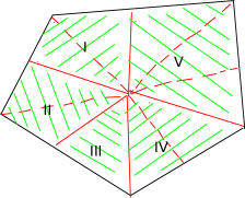
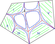
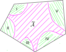
Figure 2.1. Refinement of the affine structure of [GHS] and the common enlargement $\tilde{\mathcal{A}}$ of $\mathcal{A}$ and $\Delta$. Parallel transport through the shaded areas with the same labels agrees.

In many cases, including [GS11a] and [GHK], there is an enlargement $\tilde{\mathcal{A}}$ of $\Delta_{2}\cup\mathcal{A}$ with $\Delta\subset\tilde{\mathcal{A}}$ and such that there is a deformation retraction $\tilde{\mathcal{A}}\to\Delta$. See Figure 2.1 for a sketch of a typical situation. In particular, tropical $1$-cycles on $B\setminus\Delta$ can be identified with tropical $1$-cycles on $B\setminus\tilde{\mathcal{A}}$. Replacing $\tilde{\mathcal{A}}$ by $\mathcal{A}$ then potentially allows the consideration of further tropical cycles, those that are not homologous to tropical cycles on $B\setminus\tilde{\mathcal{A}}$, that is, “passing through holes of $\mathcal{A}$”. In this sense our affine structure on $B\setminus\mathcal{A}$ is a refinement of the affine structure used in [GHS].

2.3. Construction of $n$-cycles on $X_{0}^{\circ}$ from tropical cycles on $B\setminus(\Delta_{2}\cup\mathcal{A})$

We consider tropical cycles $\beta_{\operatorname{trop}}$ as defined in Definition 1.2 for the integral affine structure from Construction 2.2. The purpose of this section is to construct an $n$-cycle $\beta$ on $X^{\circ}_{0}$ suitable for applying the results of Appendix A for the computation of the period integral $\int_{\beta}\Omega$ on $X^{\circ}_{k}$.

Assumption 2.5.

For our computation we make a few more assumptions on $\beta_{\operatorname{trop}}$ that with hindsight can be imposed without restriction and with no influence on the period integral.

1. Each point of intersection of $\beta_{\operatorname{trop}}$ with a wall is a vertex of $\beta_{\operatorname{trop}}$ and an interior point of the wall. Any edge contains at most one vertex contained in a wall.

2. Any vertex of $\beta_{\operatorname{trop}}$ of valency at least three is contained in the interior of a chamber.

3. Let $v$ be a vertex of $\beta_{\operatorname{trop}}$ contained in an $(n-1)$-cell $\rho\in\mathscr{P}$. Denote by $e$, $e^{\prime}$ the edges adjacent to $v$ with $\beta_{\operatorname{trop}}$ oriented from $e$ to $e^{\prime}$. Then $v$ is an interior point of a unique slab $\mathfrak{b}$, $v\in\mathfrak{b}\setminus\mathcal{A}$, and all vertices of $e$ and $e^{\prime}$ are bivalent. We also assume that $e$ is contained in the image under the momentum map $\mu:X_{\sigma}\to\sigma$ of the closure of an orbit of the one-dimensional algebraic torus acting on $X_{\sigma}$ and fixing the toric divisor $X_{\rho}\subset X_{\sigma}$ corresponding to $\rho$ point-wise, and similarly for $e^{\prime}$ and $\sigma^{\prime}$.

   Finally, we assume $\xi_{e}$ to be a primitive vector and if $\xi_{e}\not\in\Lambda_{\rho}$ then $\xi_{e}$ generates $\Lambda_{\sigma}/\Lambda_{\rho}$.

All these assumptions can be realized without changing the class of $\beta_{\operatorname{trop}}$ in $H_{1}(B\setminus(\Delta_{2}\cup\mathcal{A}),\Lambda)$. For example, the last assumption stated in ($\beta_{\mathrm{III}}$) can always be achieved as follows. Write $\xi_{e}=a\zeta+bm$ in $\Lambda_{\sigma}$ with $\zeta\in\Lambda_{\sigma}$ a generator of $\Lambda_{\sigma}/\Lambda_{\rho}$, $a,b\in\mathbb{Z}$ and $m\in\Lambda_{\rho}$ primitive. Then replace both $e,e^{\prime}$ by $a+b$ copies, with the first $a$ copies carrying $\zeta$ and the last $b$ copies carrying $m$. This replacement preserves the cycle property, that is, the balancing condition at vertices (2.9). A further subdivision of each new edge is needed to obtain bivalent vertices for all edges intersecting the slab.

Note in particular that each edge $e$ of our tropical cycles $\beta_{\operatorname{trop}}$ is considered a subset of $B$ and the map $h:\beta_{\operatorname{trop}}\to B$ mentioned after Definition 1.2 is defined on $e$ by the inclusion $e\to B$.

Construction 2.6.

(Construction of the $n$-cycle $\beta$ on $X_{0}^{\circ}$.) For each edge $e$ of $\beta_{\operatorname{trop}}$ let $S(e)\subseteq X_{0}^{\circ}$ be a differentiable section of $\mu$ over $e$, chosen compatibly over vertices. Note that for trivial gluing data and $\sigma$ the maximal cell containing $e$, one may choose for $S(e)$ the intersection of $\mu^{-1}(e)$ with the positive real locus of $X_{\sigma}$, but in general there is no such canonical choice. For arbitrary gluing data, we make an arbitrary choice, except if the edge $e$ has a vertex $v$ on an $(n-1)$-cell $\rho$. In this case, if $\sigma$ denotes the maximal cell containing $e$, we require $S(e)$ to be contained in the closure of an orbit of the action of the one-dimensional subtorus of $\operatorname{Spec}\mathbb{C}[\Lambda_{\sigma}]$ fixing $X_{\rho}\subset X_{\sigma}$ point-wise. Note that this condition is in agreement with the conditions imposed on $e$ in ($\beta_{\mathrm{III}}$) of Assumption 2.5. Note also that an equivalent way to state this additional condition is to ask any monomial $z^{m}\in\mathbb{C}[\Lambda_{\sigma}]$ with $m\in\Lambda_{\rho}$ to take constant values on $S(e)$.

For an edge $e$ of $\beta_{\operatorname{trop}}$ contained in a maximal cell $\sigma$ and carrying the tangent vector $\xi_{e}\in\Lambda_{\sigma}$, define $\overline{\beta}_{e}\subseteq X_{\sigma}$ as the orbit of $S(e)$ under the subgroup

(2.5) $$\tilde{T}_{e}=\big{\{}\phi\in\operatorname{Hom}(\Lambda_{\sigma},U(1))\,\big{|}\,\phi(\xi_{e})=1\big{\}}$$

of the real $n$-torus $T_{\sigma}=\operatorname{Hom}(\Lambda_{\sigma},U(1))$ acting on $X_{\sigma}$. In coordinates, the orbits of $\operatorname{Hom}(\Lambda_{\sigma},U(1))\simeq U(1)^{n}$ are the loci of constant absolute values of all monomials, that is, $|z^{m}|=\mathrm{const}$ for all $m\in\Lambda_{\sigma}$. An orbit of $\tilde{T}_{e}$ inside such an orbit is then given by $\arg(z^{\xi_{e}})=\mathrm{const}$. Note also that if $\xi_{e}$ is an $m_{e}$-fold multiple of a primitive vector $\bar{\xi}_{e}$ then $\tilde{T}_{e}$ is a product of $\mathbb{Z}/m_{e}\mathbb{Z}$ with the real $(n-1)$-torus

(2.6) $$T_{e}=\big{\{}\phi\in\operatorname{Hom}(\Lambda_{\sigma},U(1))\,\big{|}\,\phi(\bar{\xi}_{e})=1\big{\}}=\xi_{e}^{\perp}\otimes_{\mathbb{Z}}U(1).$$

The cyclic group $\mathbb{Z}/m_{e}\mathbb{Z}$ acts by multiplication by roots of unity on $z^{\bar{\xi}_{e}}$. Thus if $e$ is disjoint from all $(n-1)$-cells, $\overline{\beta}_{e}$ is topologically a disjoint union of $m_{e}$ copies of the product of an interval with $T_{e}$.

If one of the vertices $v$ of $e$ is contained in an $(n-1)$-cell $\rho$, then over $v$ one has to replace $T_{e}$ by its image $T_{e,v}=(\xi_{e}^{\perp}/\mathbb{Z}\check{d}_{\rho})\otimes_{\mathbb{Z}}U(1)$ under the restriction map

(2.7) $$\operatorname{Hom}(\Lambda_{\sigma},U(1))\longrightarrow\operatorname{Hom}(\Lambda_{\rho},U(1)).$$

Here $\check{d}_{\rho}\in\check{\Lambda}_{\sigma}=\operatorname{Hom}(\Lambda_{\sigma},\mathbb{Z})$ is a primitive normal vector to $\Lambda_{\rho}\subset\Lambda_{\sigma}$. Note that $T_{e}\to T_{e,v}$ is a finite cover of degree $|\langle\check{d}_{\rho},\xi_{e}\rangle|$ unless $\xi_{e}\in\Lambda_{\rho}$. In the latter case $T_{e}\to T_{e,v}$ contracts the circle generated by $\check{d}_{\rho}$.

To define the orientation of $\overline{\beta}_{e}$ note that $\Lambda_{\sigma}$ is oriented since $B$ is. Then $\xi_{e}$ induces a distinguished orientation on $T_{e}$ as follows. Define a basis $\bar{v}_{2},\ldots,\bar{v}_{n}$ of $\Lambda_{\sigma}/\mathbb{Z}\bar{\xi}_{e}$ to be oriented if $\bar{\xi}_{e},v_{2},\ldots,v_{n}$ is an oriented basis of $\Lambda_{\sigma}$, for any lift $v_{2},\ldots,v_{n}\in\Lambda_{\sigma}$ of $\bar{v}_{2},\ldots,\bar{v}_{n}$. Then also $\xi_{e}^{\perp}=(\Lambda_{\sigma}/\mathbb{Z}\bar{\xi}_{e})^{*}$ is oriented and in turn $T_{e}$. Now define the orientation of $\overline{\beta}_{e}$ by means of the identification

$$\overline{\beta}_{e}\simeq S_{e}\times\tilde{T}_{e}\simeq S_{e}\times T_{e}\times(\mathbb{Z}/m_{e}\mathbb{Z}),$$

with $S_{e}$ oriented by $e$. After triangulating we can view $\overline{\beta}_{e}$ as a singular chain. If $e$ in the interior of a maximal cell is oriented from vertex $v_{-}$ to $v_{+}$, the boundary $\partial\overline{\beta}_{e}$ decomposes as follows:

(2.8) $$\partial\overline{\beta}_{e}=\partial_{+}\overline{\beta}_{e}-\partial_{-}\overline{\beta}_{e},\quad\partial_{+}\overline{\beta}_{e}=\{v_{+}\}\times\tilde{T}_{e},\ \partial_{-}\overline{\beta}_{e}=\{v_{-}\}\times\tilde{T}_{e}.$$

If $e$ intersects the codimension one cell $\rho$ in one of the vertices $v_{\pm}$, the same formula holds with the factor $\tilde{T}_{e}$ in the boundary component over $v_{\pm}$ replaced by the image $\tilde{T}_{e,{v_{\pm}}}$ under the map (2.7) above, with multiplicity $|\langle\check{d}_{\rho},\xi_{e}\rangle|$. In particular, for $\xi_{e}\in\Lambda_{\rho}$, we have $\partial_{\pm}\overline{\beta}_{e}=0$ for the appropriate index $\pm$.

In any case, if $v\in\beta_{\operatorname{trop}}$ is a vertex of valency two with adjacent edges $e,e^{\prime}$ ordered according to the orientation of $\beta_{\operatorname{trop}}$, then $\partial_{+}\overline{\beta}_{e}=\partial_{-}\overline{\beta}_{e^{\prime}}$, so these two parts of the boundary cancel in $\partial(\overline{\beta}_{e}+\overline{\beta}_{e^{\prime}})$.

By ($\beta_{\textrm{II}}$), a vertex $v$ of valency at least three is contained in the interior of a maximal cell $\sigma$. Denote by $S(v)$ the point of intersection of $S(e)$ with $\mu^{-1}(v)$, for any edge $e$ adjacent to $v$. As discussed above, $\tilde{T}_{e}\cdot S(v)$ is a union of translations of the $(n-1)$-dimensional subtorus $T_{e}$ of $\mu^{-1}(v)=\operatorname{Hom}(\Lambda_{\sigma},U(1))$. The class of $\tilde{T}_{e}$ in $H_{n-1}(\mu^{-1}(v),\mathbb{Z})$ is Poincaré-dual to $\xi_{e}\in\Lambda_{\sigma}=H^{1}(\mu^{-1}(v),\mathbb{Z})$. Define $\varepsilon_{e,v}=1$ if $\tilde{T}_{e}\cdot S(v)$ is positively oriented as part of the boundary of $\overline{\beta}_{e}$ and $\varepsilon_{e,v}=-1$ otherwise. By (2.8) we have $\varepsilon_{e,v}=1$ if $e$ is oriented toward $v$. Now the balancing condition for $\beta_{\operatorname{trop}}$ at $v$ says

(2.9) $$\sum_{e\ni v}\varepsilon_{e,v}\xi_{e}=0.$$

Hence $\sum_{e\ni v}\varepsilon_{e,v}\cdot[\tilde{T}_{e}\cdot S(v)]=0$ in $H_{n-1}(\mu^{-1}(v),\mathbb{Z})$. Thus there exists an $n$-chain $\Gamma_{v}\subset\mu^{-1}(v)$ whose boundary equals the negative of this sum. The chain $\Gamma_{v}$ is unique up to adding integral multiples of $\mu^{-1}(v)$. For brevity of notation we define $\Gamma_{v}=0$ if $v$ is a bivalent vertex. By construction, the sum of chains $\sum_{e}\overline{\beta}_{e}+\sum_{v}\Gamma_{v}$ defines an $n$-cycle on $X_{0}^{\circ}$.

To arrive at a cycle of the form treated in Construction A.3, we may need to adjust some of the boundary components of edges adjacent to slabs, as will become clear in the proof of Lemma 2.7 below. To this end we admit the insertion of chains on some of such edges as follows. Let $v$ be a vertex contained in a slab and $e$, $e^{\prime}$ the adjacent edges, with $\beta$ oriented from $e$ to $e^{\prime}$. We now admit to subtract from $\overline{\beta}_{e^{\prime}}$ a chain $\Gamma_{e^{\prime}}$, while adding $\Gamma_{e^{\prime}}$ in the chart $\operatorname{Spec}R^{k}_{\mathfrak{u}^{\prime}}$ defined the chamber $\mathfrak{u}^{\prime}$ containing $e^{\prime}$ to the collection of chains. For notational convenience we define $\Gamma_{e}=0$ for all other edges $e$ and $\Gamma_{v}=0$ for all two-valent vertices $v$. The resulting chain for any edge $e$ (modified or not) is now denoted $\beta_{e}$. Thus we have $\beta_{e}=\overline{\beta}_{e}$ unless $e$ is oriented away from a vertex $v_{-}$ lying on a slab.

Finally we define

(2.10) $$\beta:=\sum_{e}\beta_{e}+\sum_{v}\Gamma_{v}+\sum_{e}\Gamma_{e}.$$

It follows from the construction that $\partial\beta=0$, so $\beta$ is a singular cycle on $X_{0}^{\circ}$. Up to specifying the slab add-ins $\Gamma_{e^{\prime}}$ in Lemma 2.7 below, this ends the construction of $\beta$.

To decompose $\beta$ in the form $\sum_{i}\beta_{i}$ demanded in Construction A.3, take for the constituents $\beta_{i}$ one of the following.

1. $\beta_{e}$ with $e$ disjoint from $(n-1)$-cells;

2. $\Gamma_{v}$ for $v$ a vertex of valency at least three;

3. The sum $\beta_{e}+\beta_{e^{\prime}}$ for the two edges $e,e^{\prime}$ adjacent to a vertex $v$ contained in an $(n-1)$-cell;

4. A slab add-in $\Gamma_{e^{\prime}}$ whenever this chain is non-zero.

Lemma 2.7.

For a cycle $\beta=\sum_{i}\beta_{i}$ from Construction 2.6 there exist charts $\Phi_{i}:\tilde{U}_{i}\to X_{k}^{\circ}$ and a choice of slab add-ins $\Gamma_{e^{\prime}}$, such that the charts $\Phi_{i}$ and chains $\beta_{i}$ fulfill (Ch I), (Ch II) and (Cy I), (Cy II) of Construction A.3, respectively.

Proof. Step I: Construction of adapted charts. By ($\beta_{\mathrm{I}}$) of Assumption 2.5 for the tropical cycle $\beta_{\operatorname{trop}}$, the constituents of the form $\beta_{i}=\beta_{e}$ or $\beta_{i}=\Gamma_{v}$ are contained in a single chamber $\mathfrak{u}$. Denote by $\sigma$ the maximal cell containing $\mathfrak{u}$. As explained in §1.1.4, the chart of $X_{k}^{\circ}$ defined by $\mathfrak{u}$ provides an open embedding

(2.11) $$\operatorname{Spec}R^{k}_{\mathfrak{u}}=\operatorname{Spec}\big{(}\mathbb{C}[\Lambda_{\sigma}]\big{)}\times O_{k}\longrightarrow X_{k}^{\circ},$$

which, viewed as a morphism of analytic log spaces, we take for $\Phi_{i}$. Thus $\tilde{U}_{i}=\operatorname{Spec}\big{(}\mathbb{C}[\Lambda_{\sigma}]\big{)}\times O_{k}$. Here we write $O_{k}=\operatorname{Spec}\mathbb{C}[t]/(t^{k+1})$ as in Appendix A. The reduction $U_{i}$ of $\tilde{U}_{i}$ is isomorphic to $(\mathbb{C}^{*})^{n}$. In the notation of Construction A.3, such $\Phi_{i}$ are charts of type I.

In the third instance of two edges $e,e^{\prime}$ with $\beta_{i}=\eta_{e}+\beta_{e^{\prime}}$ and $\beta_{\operatorname{trop}}$ oriented from $e$ to $e^{\prime}$ and meeting in a vertex $v$ on a slab $\mathfrak{b}\subseteq\underline{\rho}$, by (1.2) we similarly have an open embedding

$$\operatorname{Spec}R^{k}_{\mathfrak{b}}\longrightarrow X_{k}^{\circ},$$

with $R^{k}_{\mathfrak{b}}=CC[\Lambda_{\mathfrak{b}}][\tilde{Z}_{+},\tilde{Z}_{-},t]/(\tilde{Z}_{+}\tilde{Z}_{-}-z^{-m_{v}}f_{\mathfrak{b}}t^{\kappa_{i}},t^{k+1})$, $\kappa_{i}=\kappa_{\underline{\rho}_{\mathfrak{b}}}$. Here we use the adapted coordinates $\tilde{Z}_{\pm}$ from (2.4) with $\tilde{\zeta}=\pm\xi_{e}$ in case $\xi_{e}\not\in\Lambda_{\rho}$. Denote also by $\mathfrak{u},\mathfrak{u}^{\prime}$ and $\sigma,\sigma^{\prime}$ the chambers and maximal cells containing the images of $e,e^{\prime}$, respectively.

To bring the ring $R^{k}_{\mathfrak{b}}$ into the form required by (Ch II) of Construction A.3, we now set

(2.12) $$z=\tilde{Z}_{+},\quad w=\tilde{Z}_{-}/(z^{-m_{v}}f_{\mathfrak{b}}),$$

to obtain an open embedding of the open neighborhood $\operatorname{Spec}(R^{k}_{\mathfrak{b}})_{f_{\mathfrak{b}}}\subseteq\operatorname{Spec}R^{k}_{\mathfrak{b}}$ of $\mu^{-1}(v)$ into

(2.13) $$\operatorname{Spec}\big{(}\mathbb{C}[\Lambda_{\rho}][z,w,t]/(zw-t^{\kappa_{i}},t^{k+1})\big{)}.$$

A further shrinking of neighborhood leads to the desired chart of the form $\tilde{U}_{i}=V_{i}\times H_{\kappa_{i}}$ with $V_{i}\subset\operatorname{Hom}(\Lambda_{\mathfrak{b}},\mathbb{C}^{*})\simeq(\mathbb{C}^{*})^{n-1}$ open and $H_{\kappa_{i}}$ the base change to $O_{k}$ of an appropriate bounded open subset of $\big{\{}(z,w,t)\in\mathbb{C}^{3}\big{|}\,zw=t^{\kappa_{i}}\big{\}}$. With the possible rescaling of $z,w$ from Remark A.4 understood, this is a chart of type II with $\kappa_{i}=\kappa_{i}$. Denote by $\sigma$ the maximal cell containing $e$, and by $\sigma^{\prime}$ the other maximal cell adjacent to $\mathfrak{b}$.

Note also that the projection $V_{i}\times H_{\kappa_{i}}\to V_{i}$ is a restriction of the map

(2.14) $$\operatorname{Spec}R^{k}_{\mathfrak{b}}\longrightarrow\operatorname{Spec}\mathbb{C}[\Lambda_{\rho}]$$

induced by the inclusion $\Lambda_{\rho}\subset\Lambda_{\sigma}$, and this map is equivariant for the homomorphism of tori $T_{e}\to T_{e,v}$ discussed in Construction 2.6. By construction, $S(e)$ lies in the fiber of this projection since any monomial $z^{m}$ with $m\in\Lambda_{\rho}$ is constant on $S(e)$.

Step II: Checking (Cy I),(Cy II) for $\beta_{e}=\bar{\beta}_{e}$ and for $\Gamma_{v}$. We need to check that $\beta_{i}$ is of the form specified in (Cy II) of Construction A.3. This discussion is entirely on the central fiber $X_{0}^{\circ}$, with the toric local model $\mathbb{C}[\Lambda_{\sigma^{\prime}}]=\mathbb{C}[\Lambda_{\rho}][\tilde{Z}_{-}^{\pm 1}]$ and the non-toric one $\mathbb{C}[\Lambda_{\rho}][z,w]/(zw)$.

Condition (Cy I) is readily fulfilled if $\beta_{i}=\beta_{e}$ and $e$ is disjoint from all slabs and for $\beta_{i}=\Gamma_{v}$. It remains to consider the case $\beta_{i}=\beta_{e}$ and $e\cap\rho\neq\emptyset$ for some $\rho$.

The part $\beta_{e}$ of $\beta_{i}$ lying over $\sigma$ is again easily seen to be of the required form, with the added flexibility of Remark A.4 understood:

(i) If $\xi_{e}\in\Lambda_{\rho}$ then the action of the $(n-1)$-torus $\tilde{T}_{e}=T_{e}$ defined in (2.5) on $\mathbb{C}[\Lambda_{\rho}]$ has a one-dimensional kernel, while the action on $z=\tilde{Z}_{+}$ is non-trivial. Hence, in the chart (2.13), we have $\beta_{e}=\gamma_{i}\times\big{\{}|z|\leq\varepsilon_{i}\big{\}}$ with $\gamma_{i}$ an $(n-2)$-dimensional orbits of the action of $T_{e,v}\simeq U(1)^{n-1}$ on $\operatorname{Spec}\mathbb{C}[\Lambda_{\rho}]\simeq(\mathbb{C}^{*})^{n-1}$ and some $\varepsilon_{i}\in\mathbb{R}_{>0}$. We do not bother to compute $\gamma_{i}$ explicitly because our integral over such chains vanishes in any case.

(ii) If $\xi_{e}\not\in\Lambda_{\rho}$ then $\xi_{e}=\pm\tilde{\zeta}$. Hence the action of $\tilde{T}_{e}=T_{e}$ is trivial on $z=\tilde{Z}_{+}$ and the restriction map $T_{e}\to T_{e,v}$ of (2.7) is an isomorphism. Thus $\beta_{e}=\gamma_{i}\times z(S(e))$ with $\gamma_{i}$ a $T_{e}$-orbit and $z(S(e))$ a curve inside $\mathbb{C}$ connecting $z\big{(}S(v_{-})\big{)}$ to $0$ for $v_{-}$ the other vertex of $e$.

Step III: Construction of $\beta_{e^{\prime}}$. The situation for the other constituent $\beta_{e^{\prime}}$ of $\beta_{i}$ is less straightforward. Recall that $\beta_{e^{\prime}}=\overline{\beta}_{e^{\prime}}-\Gamma_{e^{\prime}}$ with $\overline{\beta}_{e^{\prime}}$ constructed above via the torus action and the momentum map $\mu$, while the slab add-in $\Gamma_{e^{\prime}}$ was still to be determined. Denote by $v_{+}$ the vertex of $e^{\prime}$ mapping to the interior of $\sigma^{\prime}$, the maximal cell containing $e^{\prime}$. By construction, $\overline{\beta}_{e^{\prime}}$ has the boundary component $\partial_{+}\overline{\beta}_{e^{\prime}}$ mapping to $v_{+}$ by the momentum map. This boundary component $\partial_{+}\overline{\beta}_{e^{\prime}}$ is the torus orbit $T_{e^{\prime}}\cdot S(v_{+})=\tilde{T}_{e^{\prime}}\cdot S(v_{+})$ in $\operatorname{Hom}(\Lambda_{\sigma^{\prime}},\mathbb{C}^{*})$, the reduction modulo $t$ of the chart $\operatorname{Spec}R^{k}_{\mathfrak{u}^{\prime}}$.

For the following discussion, let $e_{1},\ldots,e_{n}\in\Lambda_{\sigma^{\prime}}$ be an oriented basis with $e_{1}=\tilde{\zeta}^{\prime}$ the parallel transport of $-\tilde{\zeta}\in\Lambda_{\sigma}$ through $v$, and $e_{2},\ldots,e_{n}\in\Lambda_{\rho}$, and let $\hat{z}_{1},\ldots,\hat{z}_{n}\in R^{k}_{\mathfrak{u}^{\prime}}$ denote the corresponding monomials. Then $T_{e^{\prime}}$ is identified with a subtorus of $U(1)^{n}$ acting diagonally on $\hat{z}_{1},\ldots,\hat{z}_{n}$. For $\theta\in T_{e^{\prime}}$ denote by $(\theta_{1},\ldots,\theta_{n})$ the corresponding image in $U(1)^{n}$, with $U(1)=\big{\{}z\in\mathbb{C}\,\big{|}\,|z|=1\big{\}}$.

In these coordinates, $\partial_{+}\overline{\beta}_{e^{\prime}}$ has the parametrization

$$T_{e^{\prime}}\ni\theta=(\theta_{1},\ldots,\theta_{n})\longmapsto\theta\cdot a=\big{(}\theta_{1}a_{1},\theta_{2}a_{2},\ldots,\theta_{n}a_{n}\big{)},$$

with $a_{\mu}=\hat{z}_{\mu}\big{(}S(v_{+})\big{)}$ for $\mu=1,\ldots,n$ and $a=(a_{1},\ldots,a_{n})$.

On the other hand, Condition (Cy II) of Construction A.3 tells us that $\beta_{e^{\prime}}$ must be homologous relative to its boundary to the chain $\hat{\beta}_{e^{\prime}}$ defined analogously, but using the chart $\Phi_{i}$ modeled on $\mathbb{C}[\Lambda_{\rho}][z,w]/(zw-t^{\kappa_{i}},t^{k+1})$ and $w$ replacing $\hat{z}_{1}$. Explicitly, in the coordinates $w,z_{2},\ldots,z_{n}$ of the chart $\Phi_{i}$, with $z_{2},\ldots,z_{n}$ defined by $e_{2},\ldots,e_{n}\in\Lambda_{\rho}$, the chain $\hat{\beta}_{e^{\prime}}$ is defined by the parametrization

(2.15) $$S(e^{\prime})\times T_{e^{\prime}}\longrightarrow(\mathbb{C}^{*})^{n},\quad(p,\theta)\longmapsto\big{(}\theta_{1}w(p),\theta_{2}z_{2}(p),\ldots,\theta_{n}z_{n}(p)\big{)}.$$

The two sets of coordinates are related by

(2.16) $$c_{1}\hat{z}_{1}=(f_{\mathfrak{b}}/z^{m_{v}})\,w,\quad c_{2}\hat{z}_{2}=z_{2},\ldots,c_{n}\hat{z}_{n}=z_{n},$$

with constants $c_{\mu}=s_{\sigma^{\prime}\underline{\rho}}(e_{\mu})\in\mathbb{C}^{*}$ given by gluing data. The action of $U(1)^{n}$ on $z_{2},\ldots,z_{n}$ is compatible with the action on $\hat{z}_{2},\ldots,\hat{z}_{n}$, but not so on $w$. Let $\hat{f}_{\mathfrak{b}}\in\mathbb{C}[t][\hat{z}_{2},\ldots,\hat{z}_{n}]$ be a Laurent polynomial with the property that the reduction of $\hat{z}^{-m_{v}}\hat{f}_{\mathfrak{b}}$ modulo $t^{k+1}$ is the image of $z^{-m_{v}}f_{\mathfrak{b}}$ under the gluing map $R^{k}_{\mathfrak{b}}\to R^{k}_{\mathfrak{u}^{\prime}}$, and denote by $\hat{f}_{\underline{\rho}}$ the reduction of $\hat{f}_{\mathfrak{b}}$ modulo $t$. Then the first equation in (2.16) can be rewritten as

(2.17) $$\hat{z}_{1}=c_{1}^{-1}(\hat{f}_{\mathfrak{b}}/\hat{z}^{m_{v}})\,w.$$

To describe $\partial_{+}\hat{\beta}_{e^{\prime}}$ only the reduction modulo $t$ is relevant and hence $f_{\mathfrak{b}}$ reduces to $f_{\underline{\rho}}$. Thus in the coordinates $\hat{z}_{1},\ldots,\hat{z}_{n}$, the boundary $\partial_{+}\hat{\beta}_{e^{\prime}}$ has the parametrization

(2.18) $$T_{e^{\prime}}\ni\theta=(\theta_{1},\ldots,\theta_{n})\longmapsto\Big{(}c_{1}^{-1}\big{(}\hat{f}_{\underline{\rho}}/\hat{z}^{m_{v}}\big{)}(\theta a)\cdot\theta_{1}b_{1},\theta_{2}a_{2},\ldots,\theta_{n}a_{n}\Big{)},$$

where $b_{1}=w\big{(}S(v_{+})\big{)}$. For simplicity of notation we view here $\hat{f}_{\underline{\rho}}/\hat{z}^{m_{v}}$ as a Laurent polynomial in $n$ variables by the inclusion $\Lambda_{\rho}\subset\Lambda_{\sigma^{\prime}}$.

Step IV: Construction of slab add-ins $\Gamma_{e^{\prime}}$. Now that we have explicit parametrizations of both $\partial\hat{\beta}_{e^{\prime}}$ and $\partial\bar{\beta}_{e^{\prime}}$, we are ready to construct the slab add-in $\Gamma_{e^{\prime}}$ as a chain connecting these boundary cycles. Note that the factor in the first entry of the right-hand side of (2.18) agrees with the restriction of $f_{\underline{\rho}}/z^{m_{v}}$ on the fiber of the momentum map $\mu:X_{0}^{\circ}\to B$ over $v$:

$$\big{(}\hat{f}_{\underline{\rho}}/\hat{z}^{m_{v}}\big{)}(\theta a)=\big{(}\hat{f}_{\underline{\rho}}/\hat{z}^{m_{v}}\big{)}(\theta_{2}a_{2},\ldots,\theta_{n}a_{n})=\big{(}f_{\underline{\rho}}/z^{m_{v}}\big{)}\big{(}\theta_{2}b_{2},\ldots,\theta_{n}b_{n}\big{)},$$

with $b_{2}=z_{2}(S(v)),\ldots,b_{n}=z_{n}(S(v))$. The point is that, by the definition of $m_{v}$ in Construction 2.2, this map is homotopically trivial as a map $T_{e^{\prime}}\to\mathbb{C}^{*}$. Thus there is a differentiable homotopy $\gamma:[0,1]\times T_{e^{\prime}}\longrightarrow\mathbb{C}^{*}$ with

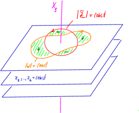
Figure 2.2. A slab add-in (case $\xi_{e^{\prime}}\in\Lambda_{\rho}$)

(2.19) $$\gamma(0,\theta)=\big{(}\hat{f}_{\underline{\rho}}/\hat{z}^{m_{v}}\big{)}(\theta a),\quad\gamma(1,\theta)=a_{1}c_{1}/b_{1},$$

where $a_{1}=\hat{z}_{1}\big{(}S(v_{+})\big{)}$, $b_{1}=w\big{(}S(v_{+})\big{)}$ and $c_{1}=s_{\sigma^{\prime}\underline{\rho}}(\tilde{\zeta}^{\prime})$. We now define the slab add-in $\Gamma_{e^{\prime}}$ in the coordinates $\hat{z}_{1},\ldots,\hat{z}_{n}$ of $R^{k}_{\mathfrak{u}^{\prime}}$ by the parametrization
$\displaystyle\hskip 34.44434pt[0,1]\times T_{e^{\prime}}\longrightarrow\operatorname{Hom}(\Lambda_{\sigma^{\prime}},\mathbb{C}^{*})$ $\displaystyle(s,\theta)\longmapsto\big{(}\gamma(s,\theta)\cdot\theta_{1}b_{1}/c_{1},\theta_{2}a_{2},\ldots,\theta_{n}a_{n}\big{)},$
with the given orientation of the domain. Figure 2.2 provides a sketch for the case $\xi_{e^{\prime}}\in\Lambda_{\rho}$. The horizontal planes indicate the level sets of $\hat{z}_{2},\ldots,\hat{z}_{n}$, which for both $\overline{\beta}_{e^{\prime}}$ and $\hat{\beta}_{e^{\prime}}$ vary in the same $U(1)^{n-2}$-orbit, the orbit containing $(\hat{z}_{2},\ldots,\hat{z}_{n})\big{(}S(v_{+})\big{)}=(\hat{z}_{2},\ldots,\hat{z}_{n})(S(e^{\prime}))$. The shaded region is the part of $\Gamma_{e}$ in this level set. The circle and curve show the intersection of $\partial_{+}\overline{\beta}_{e^{\prime}}$ and $\partial_{+}\hat{\beta}_{e^{\prime}}$ with one of the level sets in this $U(1)^{n-2}$-orbit. In the other case $\xi_{e^{\prime}}\not\in\Lambda_{\rho}$ there is a $U(1)^{n-1}$-orbit of level sets and on each level set in this orbit, $\partial_{+}\overline{\beta}_{e^{\prime}}$, $\partial_{+}\hat{\beta}_{e^{\prime}}$ define two points in the $\hat{z}_{1}$-plane, connected by the homotopy $\gamma$.

By construction, $\partial\Gamma_{e^{\prime}}=\partial_{+}\overline{\beta}_{e^{\prime}}-\partial_{+}\hat{\beta}_{e^{\prime}}$ and hence $\beta_{e^{\prime}}=\overline{\beta}_{e^{\prime}}-\Gamma_{e^{\prime}}$ has boundary $\partial_{+}\hat{\beta}_{e^{\prime}}-\partial_{-}\overline{\beta}_{e^{\prime}}$. Letting the endpoint $S(v_{+})$ vary as $s\in S(e^{\prime})$, $\gamma$ can be extended to a continuous family $\gamma_{s}$ of homotopies between the $T_{e^{\prime}}$-orbits in $\overline{\beta}_{e^{\prime}}$ and in $\hat{\beta}_{e^{\prime}}$ containing $s$. The corresponding family of $n$-chains sweeps out an $(n+1)$-chain $\tilde{\Gamma}$ with

$$\partial\tilde{\Gamma}=\overline{\beta}_{e^{\prime}}-\Gamma_{e^{\prime}}-\hat{\beta}_{e^{\prime}}.$$

Thus $\beta_{e^{\prime}}$ and $\hat{\beta}_{e^{\prime}}$ are homologous relative to their boundaries as needed in (Cy II).

We add the slab add-in $\Gamma_{e^{\prime}}$ as an additional chain, taken inside the chart (2.11) for the chamber $\mathfrak{u}^{\prime}$ containing $e^{\prime}$. With this definition for the slab add-ins, we have verified the requirements of Construction A.3 for all constituents $\beta_{i}$ of $\beta$. ∎

Proposition 2.8.

Let $\mathcal{X}\to\mathbb{D}$ be a family with $X_{0}^{\circ}$ as central fiber and locally analytically isomorphic to (1.4), together with a family of $n$-cycles $\beta(t)$ with $\beta(0)=\beta$ as in Proposition A.6. Then the Picard-Lefschetz monodromy $T$ along a counter-clockwise loop in $\mathbb{D}$ based at $t_{0}\neq 0$ acting on $n$-homology classes is given by

$$(T-\operatorname{id})(\beta_{t_{0}})=\langle c_{1}(\varphi),\beta_{\operatorname{trop}}\rangle\cdot[\alpha]=\sum_{i}\kappa_{i}\langle\check{d}_{\rho_{i}},\xi_{i}\rangle[\alpha].$$

Here $\alpha$ denotes the vanishing cycle and the sum is over the points $v$ of intersection of $\beta_{\operatorname{trop}}$ with codimension one cells $\rho=\rho_{i}$ as explained in §1.2.5.

Proof.

We apply Lemma A.7 to the specific situation laid out in the proof of Lemma 2.7. This already justifies what we are summing over. For each summand, we are in the situation (ii) stated in Step II of the proof, where $\xi_{e}\not\in\Lambda_{\rho}$ and $\beta_{e}=\gamma_{i}\times z(S(e))$. A clockwise loop in the $w$-plane gives a counter-clockwise loop in the $z$-plane, call this $S^{1}$. Hence, by Lemma A.7, $(T-\operatorname{id})(\beta_{e}+\beta_{e^{\prime}})=\kappa_{i}[\gamma_{i}\times S^{1}]$, on the level of chains up to homology. The vanishing cycle $\alpha$ is represented by an orbit of the diagonal action of $U(1)^{n}$ in the coordinates $z^{\xi_{e}},z_{2},\ldots,z_{n}$ obtained from an oriented basis $\xi_{e},e_{2},\ldots,e_{n}$ with $e_{j}\in\Lambda_{\rho}$. Relating this orbit to $\gamma_{i}\times S^{1}$, we have $z=z^{\varepsilon\xi_{e}}$ for $\varepsilon=\langle\check{d}_{\rho},\xi_{e}\rangle=\pm 1$. Recall that $\gamma_{i}$ is a $T_{e}$-orbit, so taken together with $S^{1}$, the circle in the $z$-plane, this cycle is indeed homologous to $\alpha$ up to sign. The signs work out as stated. ∎

3. Computation of the period integrals

The purpose of this section is to prove Theorem 1.7. We continue to use the setup from Section 2. In particular, we have $X_{k}^{\circ}$, an $n$-dimensional log scheme over $O_{k}=\operatorname{Spec}\mathbb{C}[t]/(t^{k+1})$ with restriction to $X_{k}^{\circ}\setminus Z$ log smooth over $O_{k}$. Here $O_{k}$ is given the log structure induced from the toric log structure on $\operatorname{Spec}\mathbb{C}[t]$. Denote by $\Omega^{n}_{X_{k}^{\circ}/O_{k}}$ the sheaf of relative log differentials of degree $n$, which is locally free away from $Z$. The construction of $X_{k}^{\circ}$ comes with a canonical relative logarithmic $n$-form $\Omega\in\Gamma(X_{k}^{\circ},\Omega^{n}_{X_{k}^{\circ}/O_{k}})$. If $\sigma$ is a maximal cell and $e_{1},\ldots,e_{n}$ is an oriented lattice basis of $\Lambda_{\sigma}$, then, in the corresponding local coordinates $z_{1}=z^{e_{1}},\ldots,z_{n}=z^{e_{n}}$ of $\operatorname{Spec}(R^{k}_{\sigma})=\operatorname{Spec}\big{(}\mathbb{C}[t,z_{1},\ldots,z_{n}]/(t^{k+1})\big{)}$, it holds

(3.1) $$\Omega=\operatorname{dlog}z_{1}\wedge\ldots\wedge\operatorname{dlog}z_{n}=z_{1}^{-1}dz_{1}\wedge\ldots\wedge z_{n}^{-1}dz_{n}.$$

We often also work with polar coordinates $z_{j}=r_{j}e^{\sqrt{-1}\alpha_{j}}$. To avoid cluttering some formulas with exponentials, we work with $\theta_{j}=e^{\sqrt{-1}\alpha_{j}}\in U(1)=S^{1}$ rather than with $\alpha_{j}\in\mathbb{R}/2\pi$, as already in the proof of Lemma 2.7. In particular, $\operatorname{dlog}z_{j}=\operatorname{dlog}r_{j}+\sqrt{-1}d\alpha_{j}$ now reads $\operatorname{dlog}z_{j}=\operatorname{dlog}r_{j}+\operatorname{dlog}\theta_{j}$ and it holds

(3.2) $$\int_{S^{1}}\operatorname{dlog}\theta_{j}=\sqrt{-1}\int_{S^{1}}d\alpha_{j}=2\pi\sqrt{-1}.$$

Recall that $Z$ intersected with the interior of a codimension one stratum $X_{\rho}\cap X_{0}^{\circ}\subset X_{0}^{\circ}$ is given by the zero locus of $f_{\underline{\rho}}$, the reduction of $f_{\mathfrak{b}}$ modulo $t$ for any slab $\mathfrak{b}\subseteq\underline{\rho}\subset\rho$. In Construction 2.2 we defined an adapted affine structure on $B\setminus(\Delta_{2}\cup\mathcal{A})$ for $\mathcal{A}=\mu(Z)$ the image of $Z$ under the generalized momentum map $\mu:X_{0}^{\circ}\to B$. For a tropical cycle $\beta_{\operatorname{trop}}$ on $B\setminus(\Delta_{2}\cup\mathcal{A})$ fulfilling Assumption 2.5 and $\beta$ the associated $n$-cycle from Construction 2.6, we now compute $\int_{\beta}\Omega$ in the form $h+g\log t$ with $h,g\in\mathbb{C}[t]/(t^{k+1})$ following Appendix A.

We first compute the period of $\Omega$ over a general fiber of the momentum map $\mu:X_{0}^{\circ}\to B$ of Proposition 2.1.

Lemma 3.1.

Let $v\in B$ be contained in the interior of a maximal cell $\sigma$ and $\alpha=\mu^{-1}(v)$, viewed as an $n$-cycle in $X_{0}^{\circ}$ with the natural orientation. Then, in the sense of finite order period integrals (Construction A.3),

$$\int_{\alpha}\Omega=(2\pi\sqrt{-1})^{n}\in\mathbb{C}[t]/(t^{k+1}).$$

Proof.

The cycle $\alpha$ is contained in a single chart $\tilde{U}_{1}=\operatorname{Spec}R^{k}_{\mathfrak{u}}$ of type (Ch I), for any chamber $\mathfrak{u}\subseteq\sigma$. Using (3.2), we obtain

$$\int_{\alpha}\Omega=\int_{(S^{1})^{n}}\operatorname{dlog}\theta_{1}\wedge\ldots\wedge\operatorname{dlog}\theta_{n}=(2\pi\sqrt{-1})^{n}.$$

∎

According to Proposition A.6, Lemma 3.1 proves the ambiguity of $\int_{\beta}\Omega$ up to multiples of $(2\pi\sqrt{-1})^{n}$, hence the stated well-definedness of the exponentiated period integral in Theorem 1.7.

We now turn to the computation of $\int_{\beta}\Omega$ for $\beta$ as in (2.10).

3.1. Integration over $\beta_{i}=\beta_{e}$ with $\Phi_{i}$ a chart of type I

Let $e$ be an edge of $\beta_{\operatorname{trop}}$ in the interior of a maximal cell $\sigma$, with vertices $v_{\pm}$ and $e$ oriented from $v_{-}$ to $v_{+}$. As in Construction 2.6 write $\xi_{e}=m_{e}\cdot\bar{\xi}_{e}$ with $m_{e}\in\mathbb{N}$ and $\bar{\xi}_{e}\in\Lambda_{\sigma}$ primitive. Complete $\bar{\xi}_{e}=e_{1}$ to an oriented basis $e_{1},\ldots,e_{n}$ of $\Lambda_{\sigma}$. Then the inclusion $\mathbb{Z}^{n-1}\to\Lambda_{\sigma}$ defined by $e_{2},\ldots,e_{n}$ induces an identification of $T_{e}$ with $U(1)^{n-1}$ acting diagonally on $(\mathbb{C}^{*})^{n-1}$ with coordinates $z_{2}=z^{e_{2}},\ldots,z_{n}=z^{e_{n}}$ and acting trivially on $z^{\overline{\xi}_{e}}$. Recall also from Construction 2.6 that $\beta_{e}=\overline{\beta}_{e}$ is defined as the orbit of $S(e)$ under $\tilde{T}_{e}=T_{e}\times\mathbb{Z}/m_{e}\mathbb{Z}$, with $\mathbb{Z}/m_{e}\mathbb{Z}$ acting on $z^{\overline{\xi}_{e}}$ by roots of unity.

According to Definition A.1 and (3.1), it holds

$$\Phi_{i}^{+}(\Omega)=\operatorname{dlog}z^{\bar{\xi}_{e}}\wedge\operatorname{dlog}z_{2}\wedge\ldots\wedge\operatorname{dlog}z_{n}.$$

In view of (A.6), we now compute

$$\int_{\beta_{i}}\Phi_{i}^{+}(\Omega) = \int_{S(e)\times\tilde{T}_{e}}\operatorname{dlog}z^{\overline{\xi}_{e}}\wedge\operatorname{dlog}z_{2}\wedge\ldots\wedge\operatorname{dlog}z_{n}$$

$$= \int_{S(e)\times T_{e}\times\mathbb{Z}/m_{e}\mathbb{Z}}\operatorname{dlog}z^{\overline{\xi}_{e}}\wedge\operatorname{dlog}\theta_{2}\wedge\ldots\wedge\operatorname{dlog}\theta_{n}$$

$$= (2\pi\sqrt{-1})^{n-1}\int_{S(e)\times\mathbb{Z}/m_{e}}\operatorname{dlog}z^{\overline{\xi}_{e}}$$

$$= (2\pi\sqrt{-1})^{n-1}\sum_{\nu=0}^{m_{e}-1}\Big{(}\log\big{(}\epsilon^{\nu}z^{\overline{\xi}_{e}}\big{(}S(v_{+})\big{)}\big{)}-\log\big{(}\epsilon^{\nu}z^{\overline{\xi}_{e}}\big{(}S(v_{-})\big{)}\big{)}\Big{)},$$

where $\epsilon$ denotes a primitive $m_{e}$-th root of unity. Expanding $\log(\epsilon^{\nu}z^{\overline{\xi}_{e}}(S(v_{\pm}))=\log\epsilon^{\nu}+\log z^{\overline{\xi}_{e}}(S(v_{\pm}))$, each term $\log\epsilon^{\nu}$ in the sum occurs twice with opposite signs, leaving us with an $m_{e}$-fold sum of $\log z^{\overline{\xi}_{e}}\big{(}S(v_{+})\big{)}-\log z^{\overline{\xi}_{e}}\big{(}S(v_{-})\big{)}$. Thus the sum equals the difference of $\log z^{\xi_{e}}=m_{e}\log z^{\bar{\xi}_{e}}$ at the two endpoints of $S(e)$, that is,

(3.3) $$\int_{\beta_{e}}\Omega=(2\pi\sqrt{-1})^{n-1}\Big{(}\log z^{\xi_{e}}\big{(}S(v_{+})\big{)}-\log z^{\xi_{e}}\big{(}S(v_{-})\big{)}\Big{)},$$

for $e$ oriented from $v_{-}$ to $v_{+}$.

3.2. Integration over $\Gamma_{v}$

We need the following lemma.

Lemma 3.2.

Let $\mu_{k}\subset U(1)$ denote the subgroup of $k$-th roots of unity. For any two positive integers $n$ and $m$, the subsets

$$A=\mu_{m}\cup\mu_{n}\quad\hbox{ and }\quad B=\mu_{m+n}\setminus((\mu_{m}\cup\mu_{n})\cap\mu_{m+n})$$

of $U(1)=S^{1}$ alternate, that is, following the circle, we alternately cross a point from $A$ and $B$.

Proof.

First assume $m=n$. Then we have $A=\{\exp(2\pi\sqrt{-1}\frac{2k}{2m})\mid k\in\mathbb{Z}\}$ and $B=\{\exp(2\pi\sqrt{-1}\frac{2k+1}{2m})\mid k\in\mathbb{Z}\}$ and the assertion holds. Next assume $m\neq n$. Set $d=\gcd(m,n)$. We may view the situation as a $d$-fold cover of the case where $m$ and $n$ are coprime. As the assertion transfers to the cover, we may assume that $\gcd(m,n)=1$ and then $\mu_{m}\cap\mu_{n}=\{1\}$ and $\operatorname{lcm}(m+n,n)=n(m+n)$ and $\operatorname{lcm}(m+n,m)=m(m+n)$. Hence

$$\mu_{m+n}\cap(\mu_{m}\cup\mu_{n})=\{1\},$$

so in particular $A$ and $B$ have the same number of elements, $m+n-1$. Now assume to the contrary of the assertion that there are consecutive elements in $B$ with no element of $A$ in between. This means there are integers $a,b,c$ such that

$$\frac{a}{m},\frac{b}{n}<\frac{c}{m+n}<\frac{c+1}{m+n}<\frac{a+1}{m},\frac{b+1}{n}.$$

Multiplying common denominators yields

$$0<(a+1)(m+n)-(c+1)m,\quad 0<(b+1)(m+n)-(c+1)n,$$

$$a(m+n)<cm,\quad b(m+n)<cn.$$

Plugging the third and fourth inequalities into the first and second, respectively, with subsequent summation of the resulting equations yields

$$0<(a+b+2)(m+n)-(c+1)(m+n)<m+n$$

which has no solution with $a,b,c\in\mathbb{Z}$. ∎

Recall the definition of $\Gamma_{v}\subset\mu^{-1}(v)=\operatorname{Hom}(\Lambda_{v},U(1))$ from Construction 2.6.

Lemma 3.3.

Let $v\in\beta_{\operatorname{trop}}$ be a vertex of valency $\upnu\geq 3$. Then

(3.4) $$\frac{1}{(2\pi\sqrt{-1})^{n}}\int_{\Gamma_{v}}\Omega=\left\{\begin{array}[]{ll}0,&\upnu\hbox{ is even,}\\ 1/2,&\upnu\hbox{ is odd.}\end{array}\right.$$

up to adding integers.

Proof. By construction, $\Gamma_{v}$ is a singular $n$-chain on the $n$-torus $\mu^{-1}(v)$. The restriction of $\Omega$ to this torus is $\operatorname{dlog}\theta_{1}\wedge\ldots\wedge\operatorname{dlog}\theta_{n}$, which agrees with $(2\pi\sqrt{-1})^{n}$ times the $U(1)^{n}$-invariant volume form $d\mathrm{vol}$ of total volume $1$. Thus the statement concerns the volume of $\Gamma_{v}$ as a fraction of the volume of $\mu^{-1}(v)$.

We have $\sum_{e\ni v}\varepsilon_{e,v}\xi_{e}=0$. Set $\xi_{j}:=\varepsilon_{e_{j},v}\xi_{e_{j}}$ for $e_{1},\ldots,e_{r}$ an enumeration of the edges containing $v$.

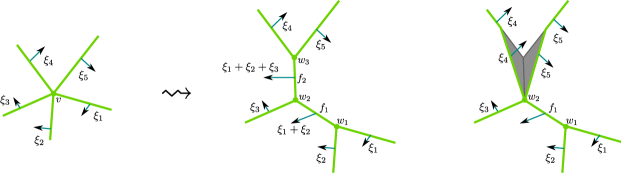
Figure 3.1. Making a vertex trivalent by the insertion of new edges and a 2-chain (in grey) that deletes one of the new edges: $f_{2}$

We decompose $v$ into trivalent vertices via insertion of $\upnu-3$ new edges $f_{1},\ldots,f_{\upnu-3}$ meeting the existing edges in the configuration, as depicted in Figure 3.1. Precisely, we replace $v$ by a chain of new edges $f_{1},\ldots,f_{\upnu-3}$ such that the ending point of $f_{j}$ is the starting point of $f_{j+1}$. Let $w_{1},\ldots,w_{\upnu-2}$ denote the vertices in this chain, the indices arranged so that $w_{1}$ meets $e_{1},e_{2}$, $w_{2}$ meets $e_{3}$, $w_{3}$ meets $e_{4}$ and so forth, finally $w_{\upnu-2}$ meets $e_{\upnu-1},e_{\upnu}$. The edge $f_{j}$ is decorated with the section $\xi_{1}+\ldots+\xi_{j+1}$. One checks that at each vertex $w_{j}$ the balancing condition (2.9) holds. One also checks that the new tropical curve is homologous to the original one. Indeed, adding boundaries of suitable 2-cycles, we can successively slide down the edges $e_{3},e_{4},\ldots$ to $w_{1}$. In this process the sections along $f_{1},\ldots,f_{\upnu-3}$ get modified and when all $e_{j}$ have been moved to the first vertex, the sections of the $f_{j}$ are all trivial and so we end up in the original setup by setting $w_{1}=v$. Since there is an injection of groups of chains

$$C_{j}(\mathbb{R}^{n},\Lambda)\to C_{j}(\mathbb{R}^{n}\times\operatorname{Hom}(\mathbb{Z}^{n},U(1))),\qquad(c,\xi)\mapsto c\times\operatorname{Hom}(\mathbb{Z}^{n}/\xi,U(1))$$

compatible with boundary maps, we conclude that the associated $n$-cycles to the original and modified $\beta_{\operatorname{trop}}$ are homologous as well. Hence

$$\int_{\Gamma_{v}}\Omega=\int_{\Gamma_{w_{1}}}\Omega+\ldots+\int_{\Gamma_{w_{\upnu-2}}}\Omega\quad\mod(2\pi\sqrt{-1})^{n}\mathbb{Z}.$$

We have reduced the assertion to the case where $v$ is trivalent. So we assume $\upnu=3$ now. As before, set $\xi_{j}:=\varepsilon_{e_{j},v}\xi_{e_{j}}$ for $j=1,2,3$. By the balancing condition (2.9), the saturated integral span $V$ of $\xi_{1},\xi_{2},\xi_{3}$ has either rank one or two. In either case, we have a product situation where we can split $\Lambda_{v}\simeq V\oplus W$ which yields a splitting of the torus

$$\operatorname{Hom}(\Lambda_{v},U(1))\simeq\operatorname{Hom}(V,U(1))\times\operatorname{Hom}(W,U(1)),$$

and $\Gamma_{v}$ also splits as $\bar{\Gamma}_{v}\times\operatorname{Hom}(W,U(1))$. The integral over the invariant volume form splits similarly with the integral over $\operatorname{Hom}(W,U(1))$ giving a factor of $1$. It remains to treat the case $\Lambda_{v}=V$.

We treat the one-dimensional case first. Let $e$ be a primitive generator of $V$ and $\xi_{j}=a_{j}e$. We have $-a_{3}=a_{1}+a_{2}$. Canceling coincidental points (as these have opposite orientation) between the multi-sets $\hat{A}=\exp(2\pi\sqrt{-1}\frac{1}{a_{1}}\mathbb{Z})\cup\exp(2\pi\sqrt{-1}\frac{1}{a_{2}}\mathbb{Z})$ and $\hat{B}=\exp(2\pi\sqrt{-1}\frac{1}{a_{1}+a_{2}}\mathbb{Z})$, we obtain sets $A$ and $B$ as in the setup of Lemma 3.2. The lemma implies that $\Gamma_{v}$ up to addition of multiples of the fundamental class is homologous to a union of non-intersecting intervals with the union of endpoints being $A\cup B$. This implies that $\Gamma_{v}$ is homologous to the sum of every other interval between the pairs of points in $A\cup B$. We claim that the area of $\Gamma_{v}$ is half the area of $S^{1}$. Indeed, the sets $A$ and $B$ are both invariant under conjugation $\kappa:z\mapsto\bar{z}$. Moreover, $\kappa$ takes $\Gamma_{v}$ to the closure of its complement, so $\Gamma_{v}$ and $\kappa(\Gamma_{v})$ have the same area. Thus

$$\int_{\Gamma_{v}}d\mathrm{vol}=\frac{1}{2}\int_{S^{1}}d\mathrm{vol}=\frac{1}{2}$$

up to adding integers.

We next turn to the case where $V$ is two-dimensional. In the universal cover $V_{\mathbb{R}}^{*}=\operatorname{Hom}(V,\mathbb{R})$ of $\operatorname{Hom}(V,U(1))$, the cycles in $\operatorname{Hom}(V,U(1))$ given by requiring $\xi_{j}\mapsto 1$ for $j=1,2,3$, respectively, pull back to the infinite, discrete union of distinct straight lines $\bigcup_{j=1}^{3}(\xi_{j}^{\perp}+\mathbb{Z}^{2})$. Let $U\subset V_{\mathbb{R}}^{*}$ denote the open complement of these lines. We claim that the pullback $\tilde{\Gamma}_{v}$ of $\Gamma_{v}$ to $V_{\mathbb{R}}^{*}$ can be taken as the closure in $V_{\mathbb{R}}^{*}$ of a set of components of $U$ such that $-\tilde{\Gamma}_{v}$ is the closure of $V_{\mathbb{R}}^{*}\setminus\tilde{\Gamma}_{v}$. If this holds then by a similar argument as in the one-dimensional case we obtain $\int_{\Gamma_{v}}d\mathrm{vol}=\frac{1}{2}$ up to integers.

To see the claim, consider the map of lattices $\mathbb{Z}^{2}\to V$ mapping $e_{1}$ to $\xi_{1}$ and $e_{2}$ to $\xi_{2}$.

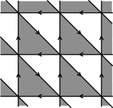
Figure 3.2. Two $\mathbb{Z}^{2}$-invariant sets of lattice triangles in $\mathbb{Z}^{2}\otimes_{\mathbb{Z}}\mathbb{R}$.

By the balancing condition, $-e_{1}-e_{2}$ then maps to $\xi_{3}$. Dually we obtain an inclusion of lattices $V^{*}\to\mathbb{Z}^{2}$ of the same index as the sublattice $\mathbb{Z}\xi_{1}+\mathbb{Z}\xi_{2}\subseteq V$. Now $\xi_{j}^{\perp}$ maps to the lines in directions $(0,1)$, $(-1,0)$ and $(1,-1)$, respectively, with the stated orientations. Together with their $\mathbb{Z}^{2}$-translations these lines subdivide $\mathbb{R}^{2}=\mathbb{Z}^{2}\otimes_{\mathbb{Z}}\mathbb{R}$ into triangular domains, see Figure 3.2: $\mathbb{Z}^{2}$-translations of the two triangles with vertices $(0,0)$, $(1,0)$, $(0,1)$ and $(1,0)$, $(1,1)$, $(0,1)$. The first triangle with the natural orientation of $\mathbb{R}^{2}$ and its $\mathbb{Z}^{2}$-translations define a $\mathbb{Z}^{2}$-invariant chain $A\subset\mathbb{R}^{2}$ with the union of lines as its boundary. Moreover, multiplication by $-1$ leads to the other triangle and its $\mathbb{Z}^{2}$-translations. Take for $\tilde{\Gamma}_{v}\subset V_{\mathbb{R}}^{*}$ the preimage of $A$ under the map $V_{\mathbb{R}}^{*}\to\mathbb{R}^{2}$. Then $\tilde{\Gamma}_{v}\cup(-\tilde{\Gamma}_{v})=V_{\mathbb{R}}^{*}$ and $\tilde{\Gamma}_{v}\cap(-\tilde{\Gamma}_{v})$ is the infinite union of lines, as claimed. ∎

3.3. Integration over $\beta_{i}=\beta_{e}+\beta_{e^{\prime}}$ with $\Phi_{i}$ a chart of type II

Let $v$ be a vertex of $\beta_{\operatorname{trop}}$ in the interior of a slab $\mathfrak{b}\subseteq\underline{\rho}$ with adjacent edges $e$, $e^{\prime}$ and $\beta_{i}=\beta_{e}+\beta_{e^{\prime}}$. We use the notation from Construction 2.6 and in addition denote $v_{-},v_{+}$ the vertices of $e,e^{\prime}$ different from $v$. The chart $\Phi_{i}$ was defined in the proof of Lemma 2.7 from $R^{k}_{\mathfrak{b}}=\mathbb{C}[\Lambda_{\mathfrak{b}}][\tilde{Z}_{+},\tilde{Z}_{-},t]/(\tilde{Z}_{+}\tilde{Z}_{-}-z^{-m_{v}}f_{\mathfrak{b}}t^{\kappa_{\underline{\rho}}},t^{k+1})$ by substituting $z=\tilde{Z}_{+}$, $w=\tilde{Z}_{-}/(z^{-m_{v}}f_{\mathfrak{b}})$. Denote by $\tilde{\zeta}\in\Lambda_{\sigma}$ the exponent with $\tilde{Z}_{+}=c_{+}z^{\tilde{\zeta}}$ for some $c_{+}\in\mathbb{C}^{*}$ as discussed in Construction 2.2 and Remark 2.3. Let $e_{1},\ldots,e_{n-1}\in\Lambda_{\rho}$ be such that $e_{1},\ldots,e_{n-1},\tilde{\zeta}\in\Lambda_{\sigma}$ is an oriented basis. Differing from the choice in Construction 2.6 and Lemma 2.7, we now take $\tilde{\zeta}$ as the last element of the basis to turn our cycles into the form required in Appendix A. In these coordinates, the logarithmic $n$-form $\Omega$ reads

$$\Omega=\operatorname{dlog}z_{1}\wedge\ldots\wedge\operatorname{dlog}z_{n-1}\wedge\operatorname{dlog}\tilde{Z}_{+}=-\operatorname{dlog}z_{1}\wedge\ldots\wedge\operatorname{dlog}z_{n-1}\wedge\operatorname{dlog}\tilde{Z}_{-},$$

and hence, since $f_{\mathfrak{b}}$ does not depend on $\tilde{Z}_{+},\tilde{Z}_{-}$,

$$\Phi_{i}^{+}(\Omega)=\operatorname{dlog}z_{1}\wedge\ldots\wedge\operatorname{dlog}z_{n-1}\wedge\operatorname{dlog}z=-\operatorname{dlog}z_{1}\wedge\ldots\wedge\operatorname{dlog}z_{n-1}\wedge\operatorname{dlog}w.$$

In the notation of (A.8), all the coefficients $g_{r},h_{r}$ of the Laurent expansion vanish and we have

$$\Phi_{i}^{+}(\Omega)=0,\quad\operatorname{res}_{\Phi_{i}}(\Omega)=\operatorname{dlog}z_{1}\wedge\ldots\wedge\operatorname{dlog}z_{n-1}.$$

Recall from Lemma 2.7 that $\beta_{e}=\overline{\beta}_{e}$, while $\beta_{e^{\prime}}=\overline{\beta}_{e^{\prime}}-\Gamma_{e^{\prime}}$ is homologous relative to its boundary to the chain $\hat{\beta}_{e^{\prime}}$ defined in (2.15). Let us first assume $\xi_{e}\not\in\Lambda_{\rho}$. Applying Formula (A.10) then gives

(3.5) $$\int_{\beta_{i}}\Omega=(-1)^{n-1}\Big{(}\int_{T_{e}}\operatorname{dlog}z_{1}\wedge\ldots\wedge\operatorname{dlog}z_{n-1}\Big{)}\big{(}\kappa_{\underline{\rho}}\log t-\log b-\log a\big{)}.$$

Here the terms with $b=w\big{(}S(v_{+})\big{)}$ and $a=z\big{(}S(v_{-})\big{)}$ adjust for $z(S(e))$ and $w(S(e^{\prime}))$ to be curves not starting or ending at $1$, see Remark A.4. The factor $(-1)^{n-1}$ comes from the fact that we oriented $\beta_{i}$ as $S(e)\times T_{e}$ rather than as $T_{e}\times S(e)$ as done in the appendix. With $\xi_{e}\not\in\Lambda_{\rho}$ we have $\xi_{e}=\overline{\xi}_{e}=\pm\tilde{\zeta}$ by ($\beta_{\mathrm{III}}$) in Assumption 2.5. Hence, up to orientation, $T_{e}$ acts as the diagonal $U(1)^{n-1}$ on $(z_{1},\ldots,z_{n-1})$. Thus by Lemma 3.1 in dimension $n-1$, the integral over $T_{e}$ equals $\pm(2\pi\sqrt{-1})^{n-1}$. To determine the sign recall that we oriented $T_{e}$ from an adapted oriented basis of $\Lambda_{\sigma}$ with first element $\overline{\xi}_{e}=\xi_{e}$. Placing $\overline{\xi}_{e}$ at the last place rather than the first changes the orientation of $T_{e}$ by $(-1)^{n-1}$, canceling the sign factor in (3.5). Finally, $\xi_{e}=\pm\tilde{\zeta}$ with the sign positive iff $\xi_{e}$ points into the maximal cell $\sigma$ containing $e$. Thus denoting by $\check{d}_{e}\in\check{\Lambda}_{\sigma}$ the generator of $\Lambda_{\rho}^{\perp}\simeq\mathbb{Z}$ with $\langle\check{d}_{e},\tilde{\zeta}\rangle=1$ we have

(3.6) $$\xi_{e}=\overline{\xi}_{e}=\langle\check{d}_{e},\overline{\xi}_{e}\rangle\cdot\tilde{\zeta}.$$

With this discussion, (3.5) yields the following:

(3.7) $$\int_{\beta_{i}}\Omega=(2\pi\sqrt{-1})^{n-1}\langle\check{d}_{e},\xi_{e}\rangle\Big{(}\kappa_{\underline{\rho}}\log t-\log w\big{(}S(v_{+})\big{)}-\log z\big{(}S(v_{-})\big{)}\Big{)}.$$

The coordinate $z=\tilde{Z}_{+}$ maps to $s_{\sigma\underline{\rho}}(\tilde{\zeta})z^{\tilde{\zeta}}$ under the generization map $R^{k}_{\mathfrak{b}}\to R^{k}_{\mathfrak{u}}$. Using (3.6) we can thus rewrite (3.7) for later use as

(3.8) $$\frac{1}{(2\pi\sqrt{-1})^{n-1}}\int_{\beta_{i}}\Omega= \langle\check{d}_{e},\xi_{e}\rangle\Big{(}\kappa_{\underline{\rho}}\log t-\log w\big{(}S(v_{+})\big{)}\Big{)}$$

$$-\log s_{\sigma\underline{\rho}}(\xi_{e})-\log z^{\xi_{e}}\big{(}S(v_{-})\big{)}.$$

In the other case, $\xi\in\Lambda_{\rho}$, our chain $\beta_{i}$ is of type (ii) in (Cy II) of Construction A.3 and $\int_{\beta_{i}}\Omega=0$ by Formula (A.10). Thus (3.8) also holds in this case because $\langle\check{d}_{e},\xi_{e}\rangle=0$.

3.4. Integration over a slab add-in $\beta_{i}=\Gamma_{e^{\prime}}$

Let $v$ be a vertex of $\beta_{\operatorname{trop}}$ mapping to a slab $\mathfrak{b}\subseteq\underline{\rho}$, with adjacent edges $e,e^{\prime}$. For the following computation we adopt the notation of the construction of a slab add-in $\Gamma_{e^{\prime}}$ in Step IV of the proof of Lemma 2.7. Formula 2.3 gives the parametrization of $\Gamma_{e^{\prime}}$ with respect to coordinates $\hat{z}_{1},\ldots,\hat{z}_{n}$ of $\operatorname{Hom}(\Lambda_{\sigma^{\prime}},\mathbb{C}^{*})$, the reduction modulo $t$ of the relevant chart $\operatorname{Spec}R^{k}_{\mathfrak{u}^{\prime}}$, where $\mathfrak{u}^{\prime}$ is the chamber containing the image of $e^{\prime}$:

$$[0,1]\times T_{e^{\prime}}\longrightarrow\operatorname{Hom}(\Lambda_{\sigma},\mathbb{C}^{*}),\quad(\theta,s)\longmapsto\big{(}\gamma(s,\theta)\cdot\theta_{1}b_{1}/c_{1},\theta_{2}a_{2},\ldots,\theta_{n}a_{n}\big{)}.$$

The map $\gamma:[0,1]\times T_{e^{\prime}}\to\mathbb{C}^{*}$ is a differentiable homotopy with

(3.9) $$\gamma(0,\theta)=(\hat{f}_{\underline{\rho}}/\hat{z}^{m_{v}})(\theta a),\quad\gamma(1,\theta)=a_{1}c_{1}/b_{1}.$$

Since the chart $\Phi_{i}$ for $\beta_{i}$ is of type (Ch I) of Construction A.10, the first case of Definition A.1 gives

$$\Phi_{i}^{+}\Omega=\operatorname{dlog}\hat{z}_{1}\wedge\ldots\wedge\operatorname{dlog}\hat{z}_{n}.$$

If $\xi_{e}\in\Lambda_{\rho}$, the period integral $\int_{[0,1]\times T_{e^{\prime}}}\Phi_{i}^{+}\Omega$ involves two-dimensional integrals over level sets of $z_{2},\ldots,z_{n}$ and hence vanishes, see Figure 2.2. In the other case $\xi_{e}\not\in\Lambda_{\rho}$, the torus $T_{e^{\prime}}$ acts trivially on $z_{1}$ and the restriction map

$$T_{e^{\prime}}\longrightarrow U(1)^{n-1},\quad\theta\longmapsto(\theta_{2},\ldots,\theta_{n})$$

is an isomorphism. Since $\hat{z}_{1}=z^{\tilde{\zeta}^{\prime}}$, this isomorphism is orientation preserving if $\xi_{e}$ points into the same maximal cell as $\tilde{\zeta}^{\prime}$, and then $\tilde{\zeta}^{\prime}=\xi_{e}$. In terms of $\check{d}_{e}\in\check{\Lambda}_{\sigma}$ used in (3.6) this is the case if and only if $\langle\check{d}_{e},\xi_{e}\rangle=-1$. We can now compute

(3.10) $$\int_{\Gamma_{e^{\prime}}}\Omega\ =\ \int_{[0,1]\times T_{e^{\prime}}}\Phi_{i}^{+}(\Omega)$$

$$=-\langle\check{d}_{e},\xi_{e}\rangle\int_{[0,1]\times U(1)^{n-1}}\partial_{s}\log\gamma(s,\theta)\,ds\wedge\operatorname{dlog}\theta_{2}\wedge\ldots\wedge\operatorname{dlog}\theta_{n}$$

$$=-\langle\check{d}_{e},\xi_{e}\rangle\int_{U(1)^{n-1}}\big{(}\log\gamma(1,\theta)-\log\gamma(0,\theta)\big{)}\,\operatorname{dlog}\theta_{2}\wedge\ldots\wedge\operatorname{dlog}\theta_{n}$$

$$=-\langle\check{d}_{e},\xi_{e}\rangle(2\pi\sqrt{-1})^{n-1}\big{(}\log(a_{1}c_{1}/b_{1})-\mathcal{R}\big{(}z^{-m_{v}}f_{\underline{\rho}},v)\big{)}.$$

As in (3.8) the sign $-\langle\check{d}_{e},\xi_{e}\rangle$ adjusts the orientation of $T_{e^{\prime}}$ with the orientation of $U(1)^{n-1}$. Note that this factor renders the formula also correct in the case $\xi_{e}\in\Lambda_{\rho}$. The last equality follows from (3.9) and the definition of the complex Ronkin function in (1.7), see §1.3.2. The term $a_{1}c_{1}/b_{1}\in\mathbb{C}^{*}$ is the constant endpoint of the homotopy $\gamma$ defined in (2.19). In the notation used there, provided $\xi_{e}\not\in\Lambda_{\rho}$, we have

$$a_{1}=\hat{z}_{1}(S(v_{+}))=z^{-\langle\check{d}_{e},\xi_{e}\rangle\xi_{e^{\prime}}}\big{(}S(v_{+})\big{)},\ \ b_{1}=w\big{(}S(v_{+})\big{)},\ \ c_{1}=s_{\sigma^{\prime}\underline{\rho}}(\tilde{\zeta}^{\prime})=s_{\sigma^{\prime}\underline{\rho}}(\xi_{e^{\prime}})^{-\langle\check{d}_{e},\xi_{e}\rangle}.$$

Thus we can write (3.10) more intrinsically as

(3.11) $$\frac{1}{(2\pi\sqrt{-1})^{n-1}}\int_{\Gamma_{e^{\prime}}}\Omega= \langle\check{d}_{e},\xi_{e}\rangle\Big{(}\mathcal{R}(z^{-m_{v}}f_{\underline{\rho}},v)+\log w\big{(}S(v_{+})\big{)}\Big{)}$$

$$+\log z^{\xi_{e^{\prime}}}\big{(}S(v_{+})\big{)}+\log s_{\sigma^{\prime}\underline{\rho}}(\xi_{e^{\prime}})$$

Note that this formula also holds if $\xi_{e}\in\Lambda_{\rho}$ and that the term $w\big{(}S(v_{+})\big{)}$ appears in (3.8) with opposite sign.

3.5. Interpolation between charts

There are two cases where we work with different charts at a vertex $v$ of $\beta$. First, if $v$ lies on a wall $\mathfrak{p}$ and the two edges $e,e^{\prime}$ adjacent to $v$ according to $(\beta_{\rm II})$ are contained in different chambers $\mathfrak{u}$, $\mathfrak{u}^{\prime}$. Second, if $v$ is adjacent to an edge intersecting a slab. In these cases there is a potentially non-trivial contribution of the interpolation term $\int_{[0,1]\times\gamma_{i}^{\mu}}\Phi_{ij}^{+}(\Omega)$ in (A.9). In all other cases, intersecting chains $\beta_{i}$ and $\beta_{j}$ lie in the interior of the same chamber and hence $\Phi_{i}=\Phi_{j}$. We now determine the contribution of the interpolation term in the remaining cases.

Let us first treat the case that $v$ lies on a wall $\mathfrak{p}$ separating chambers $\mathfrak{u}$, $\mathfrak{u}^{\prime}$. Let $\Phi_{i}:\tilde{U}_{i}\to X_{k}^{\circ}$, $\Phi_{j}:\tilde{U}_{j}\to X_{k}^{\circ}$ be the charts for the adjacent edges $e\subseteq\mathfrak{u}$, $e^{\prime}\subseteq\mathfrak{u}^{\prime}$, respectively, as defined in the proof of Lemma 2.7. Then $\tilde{U}_{i}=\tilde{U}_{j}=\operatorname{Spec}\mathbb{C}[t]/(t^{k+1})[\Lambda_{\sigma}]$ and $\Phi_{j}=\Phi_{i}\circ\Psi_{ij}$ with $\Psi_{ij}$ defined by the wall crossing isomorphism

(3.12) $$\theta_{\mathfrak{p}}:R^{k}_{\mathfrak{u}}\longrightarrow R^{k}_{\mathfrak{u}^{\prime}},\quad z^{m}\longmapsto f_{\mathfrak{p}}^{\langle\check{d}_{\mathfrak{p}},m\rangle}z^{m}.$$

Here $\check{d}_{\mathfrak{p}}\in\check{\Lambda}_{\sigma}$ is the generator of $\Lambda_{\mathfrak{p}}^{\perp}\simeq\mathbb{Z}$ evaluating positively on tangent vectors pointing from $\mathfrak{p}$ into $\mathfrak{u}$. Writing $f_{\mathfrak{p}}=1+t\tilde{f}_{\mathfrak{p}}$, the homotopy $\Phi_{ij}:[0,1]\times U_{i}\times O_{k}\to X_{k}^{\circ}$ between $\Phi_{i}$ and $\Phi_{j}$ of (A.5) can be defined by the family of $\mathbb{C}$-algebra homomorphisms

$$\theta_{\mathfrak{p}}(s):R^{k}_{\mathfrak{u}}\longrightarrow R^{k}_{\mathfrak{u}^{\prime}},\quad z^{m}\longmapsto(1+st\tilde{f}_{\mathfrak{p}})^{\langle\check{d}_{\mathfrak{p}},m\rangle}z^{m},$$

$s\in[0,1]$. Let $e_{1},\ldots,e_{n}$ be an oriented basis of $\Lambda_{\sigma}$ with $\langle\check{d}_{\mathfrak{p}},e_{1}\rangle=1$ and $e_{2},\ldots,e_{n}$ spanning $\Lambda_{\mathfrak{p}}$. Then in the corresponding coordinates $z_{1},\ldots,z_{n}$, the function $\tilde{f}_{\mathfrak{p}}$ does not depend on $z_{1}$, while $\theta_{\mathfrak{p}}(s)(z_{1})=(1+st\tilde{f}_{\mathfrak{p}})z_{1}$ and $\theta_{\mathfrak{p}}(s)(z_{\mu})=z_{\mu}$ for $\mu=2,\ldots,n$. Hence

(3.13) $$\Phi_{ij}^{+}(\Omega)=\big{(}\operatorname{dlog}z_{1}+\partial_{s}\log(1+st\tilde{f}_{\mathfrak{p}})ds\big{)}\wedge\operatorname{dlog}z_{2}\wedge\ldots\wedge\operatorname{dlog}z_{n}.$$

With $a_{i}=z_{i}(S(v))$ the coordinates of $S(e)$ over $v$, integrating out $s$, we obtain

$$\int_{[0,1]\times T_{e}}\Phi_{ij}^{+}(\Omega)\ =\ \int_{T_{e}}\log\big{(}1+t\tilde{f}_{\mathfrak{p}}(t,z_{2},\ldots,z_{n})\big{)}\operatorname{dlog}z_{2}\wedge\ldots\wedge\operatorname{dlog}z_{n}$$

$$= \int_{T_{e}}\log\big{(}1+t\tilde{f}_{\mathfrak{p}}(t,\theta_{2}a_{2},\ldots,\theta_{n}a_{n})\big{)}\operatorname{dlog}\theta_{2}\wedge\ldots\wedge\operatorname{dlog}\theta_{n}$$

Expanding the logarithm yields a finite sum of constant multiples of $t^{\ell}\theta_{2}^{\ell_{2}}\ldots\theta_{n}^{\ell_{n}}$ with $\ell,\ell_{2},\ldots,\ell_{n}\in\mathbb{N}$ and $\ell_{\mu}>0$ for at least one $\mu$. If $\xi_{e}\in\Lambda_{\mathfrak{p}}$, then similar to the situation along codimension one cells discussed in Construction 2.6, the action of $T_{e}$ on $(z_{2},\ldots,z_{n})$ has a kernel and the integral in (3.5) vanishes for trivial reasons. In the other case $\xi_{e}\not\in\Lambda_{\rho}$, the torus $T_{e}$ acts on $(z_{2},\ldots,z_{n})$ via a finite covering $T_{e}\to U(1)^{n-1}$ and the integral vanishes because $\int_{S^{1}}\theta_{\mu}^{\ell_{\mu}}\operatorname{dlog}\theta_{\mu}=0$ for an index $\mu$ with $\ell_{\mu}\neq 0$. Hence in any case, there is no interpolation contribution from changing chambers at walls.

In the second case, $\beta_{i}=\beta_{e}+\beta_{e^{\prime}}$ maps to a chart of type (Ch II). Let $e,e^{\prime}$ map to chambers $\mathfrak{u},\mathfrak{u}^{\prime}$ separated by the slab $\mathfrak{b}$ containing the common vertex $v$ of $e$ and $e^{\prime}$. As in the construction of $\beta_{i}$ in Lemma 2.7, assume $\beta$ is oriented from $e$ to $e^{\prime}$ and hence $e^{\prime}$ attaches to the non-trivial slab add-in $\Gamma_{e^{\prime}}$. Then $\beta_{e}$ was constructed with the toric coordinate $z=\tilde{Z}_{+}$ and the chart $\tilde{U}_{i}$ is compatible with $R^{k}_{\mathfrak{u}}$ in that the localization map $R^{k}_{\mathfrak{b}}\to R^{k}_{\mathfrak{u}}$ is toric. In particular, both charts provide the same local product decomposition with respect to $t$ and hence the change of coordinates map $\Psi_{ij}$ in Construction A.3 is the identity. Thus there is also no interpolation contribution from this boundary of $\beta_{i}$.

The interesting change of coordinates happens between $\beta_{e^{\prime}}$ and the slab add-in $\Gamma_{e^{\prime}}$. According to Construction A.3 we need to interpolate between the chart $\Phi_{i}:\tilde{U}_{i}\to X_{k}^{\circ}$, modeled on $\mathbb{C}[\Lambda_{\rho}][z,w,t](zw-t^{\kappa_{i}},t^{k+1})$ and used for $\beta_{e^{\prime}}$, and the chart $\Phi_{j}:\tilde{U}_{j}\to X_{k}^{\circ}$, modeled on $R^{k}_{\mathfrak{u}^{\prime}}$ and used for $\Gamma_{e^{\prime}}$. In (2.16) this change of coordinates has already been made explicit, by using toric coordinates $\hat{z}_{1},\ldots,\hat{z}_{n}$ for $\tilde{U}_{j}$ and $w,z_{2},\ldots,z_{n}$ for $\tilde{U}_{i}\setminus(w=0)$. In the notation of Construction A.3 and of (2.16)(2.17), the pull-back by $\Psi_{ij}:U_{ij}\times O_{k}\to U_{ij}\times O_{k}$ is the map

$$w\longmapsto c_{1}\hat{z}_{1}/(\hat{z}^{-m_{v}}\hat{f}_{\mathfrak{b}}),\quad z_{2}\longmapsto c_{2}\hat{z}_{2},\,\ldots,\,z_{n}\longmapsto c_{n}\hat{z}_{n},$$

while the map denoted “$\operatorname{id}$” in the appendix has the same form, but with $\hat{f}_{\mathfrak{b}}$ replaced by the reduction $f_{\underline{\rho}}$ modulo $t$. Indeed, “$\operatorname{id}$” is defined as the map $U_{ij}\times O_{k}\to U_{ij}\times O_{k}$ induced by the identity map of $U_{ij}$ as a subset of $X_{0}^{\circ}$ and extended by the product structure in the charts $\tilde{U}_{i}$ and $\tilde{U}_{j}$, respectively. Writing $\hat{f}_{\mathfrak{b}}=\hat{f}_{\underline{\rho}}+tg_{\mathfrak{b}}$, define for $s\in[0,1]$,

$$\hat{f}_{\mathfrak{b}}(s)=\hat{f}_{\underline{\rho}}+stg_{\mathfrak{b}}.$$

Then the family of maps $\Psi_{ij}(s)$, $s\in[0,1]$, defined by

(3.15) $$w\longmapsto c_{1}\hat{z}_{1}/(\hat{z}^{-m_{v}}\hat{f}_{\mathfrak{b}}(s)),\quad z_{2}\longmapsto c_{2}\hat{z}_{2},\,\ldots,\,z_{n}\longmapsto c_{n}\hat{z}_{n}$$

is a homotopy connecting $\operatorname{id}$ to $\Psi_{ij}$. Thus we can take $\Phi_{ij}(s)=\Phi_{i}^{(j)}\circ\Psi_{ij}(s)$ as the homotopy between the two restrictions of charts $\Phi_{i}^{(j)}=\Phi_{i}|_{U_{ij}\times O_{k}}$ and $\Phi_{j}^{(i)}=\Phi_{j}|_{U_{ij}\times O_{k}}$. Since $\hat{z}_{1},\ldots,\hat{z}_{n}$ was defined by an oriented basis $e_{1}=\tilde{\zeta}^{\prime},e_{2},\ldots,e_{n}$ of $\Lambda_{\sigma^{\prime}}$, replacing $\hat{z}_{1}$ by $w=c_{1}\hat{z}_{1}/(\hat{z}^{-m_{v}}\hat{f}_{\mathfrak{b}})$ shows $\Phi_{i}^{+}(\Omega)=\operatorname{dlog}w\wedge\operatorname{dlog}z_{2}\wedge\ldots\wedge\operatorname{dlog}z_{n}$. Pulling back by (3.15) then gives

$$\Phi_{ij}^{+}(\Omega)=\big{(}\operatorname{dlog}\hat{z}_{1}-\partial_{s}\log(\hat{z}^{-m_{v}}\hat{f}_{\mathfrak{b}}(s))\,ds\big{)}\wedge\operatorname{dlog}\hat{z}_{2}\wedge\ldots\wedge\operatorname{dlog}\hat{z}_{n}.$$

Similar to (3.11), the interpolation contribution to the period integral is now computed as

$$\int_{[0,1]\times T_{e^{\prime}}}\Phi_{ij}^{+}(\Omega)\ =\ \int_{T_{e^{\prime}}}\big{(}-\log(\hat{z}^{-m_{v}}\hat{f}_{\mathfrak{b}})+\log(\hat{z}^{-m_{v}}\hat{f}_{\underline{\rho}})\big{)}\,\operatorname{dlog}\hat{z}_{2}\wedge\ldots\wedge\operatorname{dlog}\hat{z}_{n}$$

$$= \langle\check{d}_{e},\xi_{e}\rangle\int_{U(1)^{n-1}}\big{(}\log(\hat{z}^{-m_{v}}\hat{f}_{\mathfrak{b}})-\log(\hat{z}^{-m_{v}}\hat{f}_{\underline{\rho}})\big{)}\,\operatorname{dlog}\theta_{2}\wedge\ldots\wedge\operatorname{dlog}\theta_{n}$$

$$= \langle\check{d}_{e},\xi_{e}\rangle(2\pi\sqrt{-1})^{n-1}\big{(}\mathcal{R}(z^{-m_{v}}f_{\mathfrak{b}},v)-\mathcal{R}(z^{-m_{v}}f_{\underline{\rho}},v)\big{)}.$$

As in (3.8), a factor $-\langle\check{d}_{e},\xi_{e}\rangle$ was inserted for the second equality to adjust for the orientation of $T_{e^{\prime}}$ and for the non-trivial kernel of the map to $U(1)^{n-1}$ in case $\xi_{e}\in\Lambda_{\rho}$, respectively.

Note that the Ronkin function for $z^{-m_{v}}f_{\underline{\rho}}$ in this result cancels with the contribution (3.11) from the slab add-in, thus only leaving the Ronkin function for $z^{-m_{v}}f_{\mathfrak{b}}$ to contribute to the global period integral.

3.6. Proof of Theorem 1.7

To compute $\frac{1}{(2\pi\sqrt{-1})^{n-1}}\int_{\beta}\Omega$, it remains to take the sum over all the computed terms. We had contributions from $\beta_{e}$ for edges disjoint from slabs (3.3), from $\Gamma_{v}$ for a vertex of higher valency (3.4), from $\beta_{i}=\beta_{e}+\beta_{e^{\prime}}$ for pairs of edges crossing a slab (3.8), from slab add-ins $\Gamma_{e^{\prime}}$ (3.11), and from interpolation terms (3.5). Note that in view of Lemma 3.1 and Proposition A.5 the result is only well-defined up to adding integral multiples of $2\pi\sqrt{-1}$.

First, for a vertex of valency ${\operatorname{val}}(v)\geq 3$ the chain $\Gamma_{v}$ contributes ${\operatorname{val}}(v)\cdot\pi\sqrt{-1}$ up to adding integral multiples of $2\pi\sqrt{-1}$. But a graph without one-valent vertices can be built inductively by successively connecting two vertices (possibly equal) by an edge. Each such addition increases $\sum_{v}{\operatorname{val}}(v)$ by $2$. Thus $\sum_{v}\int_{\Gamma_{v}}\Omega$ is a multiple of $(2\pi\sqrt{-1})^{n}$ and hence can be omitted.

The other terms are easiest to gather according to the types of vertices. For a vertex $v$ in the interior of a maximal cell $\sigma$ and each edge $e$ with vertex $v$ we have a contribution $\pm\log z^{\xi_{e}}(S(v))$ from (3.3), (3.8) or (3.11). The sign $\varepsilon_{e,v}=1$ is positive if $e$ is oriented towards $v$ and $\varepsilon_{e,v}=-1$ otherwise. By the balancing condition (2.9), the sum over all these terms vanishes:

$$\sum_{e\ni v}\log z^{\varepsilon_{e,v}\xi_{e}}=\log z^{\sum_{e\ni v}\varepsilon_{e,v}\xi_{e}}=0.$$

Collecting the remaining terms now gives

(3.17) $$\frac{1}{(2\pi\sqrt{-1})^{n-1}}\int_{\beta}\Omega$$

$$=\sum_{v}\Big{(}\langle\check{d}_{e},\xi_{e}\rangle\mathcal{R}(z^{-m_{v}}f_{\mathfrak{b}},v)+\log\frac{s_{\sigma^{\prime}\underline{\rho}}(\xi_{e^{\prime}})}{s_{\sigma\underline{\rho}}(\xi_{e})}+\langle\check{d}_{e},\xi_{e}\rangle\cdot\kappa_{\underline{\rho}}\log t\Big{)}.$$

The sum runs over all vertices $v$ of $\beta_{\operatorname{trop}}$ mapping to a slab, and in the sum $e,e^{\prime}$, $\mathfrak{b}$, $\underline{\rho}$ denote the corresponding incoming and outgoing edges, the slab containing $v$ and the corresponding codimension one cell of the barycentric subdivision, respectively. The sum over the terms containing the gluing data gives $\log\langle s,\beta_{\operatorname{trop}}\rangle$, while the sum involving $\kappa_{\underline{\rho}}$ yields

$$\sum\langle\check{d}_{e},\xi_{e}\rangle\cdot\kappa_{\underline{\rho}}=\langle c_{1}(\varphi),\beta_{\operatorname{trop}}\rangle.$$

Thus (3.17) can be written more intrinsically as

(3.18) $$\frac{1}{(2\pi\sqrt{-1})^{n-1}}\int_{\beta}\Omega$$

$$=\log\langle s,\beta_{\operatorname{trop}}\rangle+\langle c_{1}(\varphi),\beta_{\operatorname{trop}}\rangle\cdot\log t+\sum_{v}\langle\check{d}_{e},\xi_{e}\rangle\mathcal{R}(z^{-m_{v}}f_{\mathfrak{b}},v).$$

Exponentiating finally gives the expression for $\exp\big{(}(2\pi\sqrt{-1})^{-(n-1)}\int_{\beta}\Omega\big{)}$ claimed in Theorem 1.7.

4. Analyticity of formal toric degenerations

As an application of the period computations we prove analyticity of the canonical toric degenerations constructed in [GS11a] in the case that $(B,\mathscr{P})$ as simple singularities. Simple singularities are locally indecomposable from the affine geometric point of view and they give rise to locally rigid logarithmic singularities. We won’t need any details of simple singularities in this paper and refer to [GS06], Definition 1.60 for the formal definition and to [GS10], §2.2, for the local algebraic description and deformation theory. For $(B,\mathscr{P})$ with simple singularities and a choice of multivalued, strictly convex piecewise affine function $\varphi$ on $B$, it has been shown in [GS11a] and [GHS], Theorem A.2, that there is a canonical toric degeneration

(4.1) $$\mathfrak{X}\longrightarrow\mathfrak{S}=\operatorname{Spf}\big{(}A\llbracket t\rrbracket\big{)}.$$

Here $A$ is a Laurent polynomial ring, so the base of this family is the product of an algebraic torus with $\operatorname{Spf}\big{(}\mathbb{C}\llbracket t\rrbracket\big{)}$. If $\partial B\neq\emptyset$, by [GHS], Remark 2.18 and Remark 4.13, the family in (4.1) comes equipped with a divisor $\mathfrak{D}\subset\mathfrak{X}$ that is flat over $\mathfrak{S}$.

To describe the ring $A$, recall from [GS06], Theorem 5.4, that for simple singularities, the affine cohomology group $H^{1}(B,\iota_{*}\check{\Lambda}\otimes\mathbb{C}^{*})$ is canonically in bijection with the set of isomorphism classes of log schemes $(X_{0},\mathcal{M}_{X_{0}})$ over the standard log point with associated discrete data $(B,\mathscr{P},\varphi)$. The bijection works by identifying the set of isomorphism classes of log schemes with the set of equivalence classes of lifted, normalized gluing data, which in turn can be identified with the mentioned affine cohomology group. The base ring is

$$A=\mathbb{C}[H^{1}(B,\iota_{*}\check{\Lambda})^{*}],$$

the Laurent polynomial ring over $H^{1}(B,\iota_{*}\check{\Lambda})^{*}=\operatorname{Hom}(H^{1}(B,\iota_{*}\check{\Lambda}),\mathbb{Z})$. Thus $\operatorname{Spec}A$ parametrizes choices of lifted, normalized gluing data.

The construction of the family (4.1) depends on the choice of a splitting $\sigma_{0}$ of the quotient map $q_{f}:H^{1}(B,\iota_{*}\check{\Lambda})\to H^{1}(B,\iota_{*}\check{\Lambda})_{f}$ by the torsion submodule $H^{1}(B,\iota_{*}\check{\Lambda})_{t}\subseteq H^{1}(B,\iota_{*}\check{\Lambda})$. Here $\iota:B_{0}\to B$ is the inclusion of the regular locus and $\check{\Lambda}=\mathcal{H}\!\text{{om}}(\Lambda,\underline{\mathbb{Z}})$ is the sheaf of integral cotangent vectors on $B_{0}$. Such a splitting $\sigma_{0}$ is unique only up to a homomorphism $H^{1}(B,\iota_{*}\check{\Lambda})_{f}\to H^{1}(B,\iota_{*}\check{\Lambda})_{t}$. Thus if $H^{1}(B,\iota_{*}\check{\Lambda})$ has non-trivial torsion, there are finitely many such canonical families. We fix $\sigma_{0}$ and the resulting canonical family throughout this Chapter.

If $H^{2}(B,\iota_{*}\check{\Lambda})$ has torsion, the set of gluing data $H^{1}(B,\iota_{*}\check{\Lambda}\otimes\mathbb{C}^{*})$ is a disjoint union of torsors for $H^{1}(B,\iota_{*}\check{\Lambda})\otimes\mathbb{C}^{*}$, with only one of them containing trivial gluing data. Indeed, the construction of the family also depends on the choice of a possibly non-trivial element $s_{0}\in H^{1}(B,\iota_{*}\check{\Lambda}\otimes\mathbb{C}^{*})$, which selects one of these torsors. If $H^{2}(B,\iota_{*}\check{\Lambda})$ is torsion-free, trivial gluing data $s_{0}=1$ is a canonical choice. In any case, we fix $s_{0}$ throughout.

As a further ingredient in this section, recall from [GS06], Definition 1.45 (using the notation of [GHS], §A.2) that the short exact sequence

(4.2) $$0\longrightarrow\iota_{*}\check{\Lambda}\longrightarrow\breve{\mathcal{PL}}(B)\longrightarrow\breve{\mathcal{MP\!A}}(B)\longrightarrow 0,$$

gives rise to the connecting homomorphism

$$c_{1}:\breve{\operatorname{MPA}}(B)\longrightarrow H^{1}(B,\iota_{*}\check{\Lambda}).$$

This homomorphism sends a multivalued piecewise affine function $\varphi$ to its characteristic class $c_{1}(\varphi)$. Dually, we have

(4.3) $$c_{1}^{*}:H^{1}(B,\iota_{*}\check{\Lambda})^{*}\longrightarrow\breve{\operatorname{MPA}}(B)^{*}.$$

The trace homomorphism $\iota_{*}\Lambda\otimes\iota_{*}\check{\Lambda}\to\underline{\mathbb{Z}}$ combined with the sheaf homology-cohomology pairing gives a bilinear map

(4.4) $$\langle\ ,\,\rangle:H^{1}(B,\iota_{*}\check{\Lambda})\otimes H_{1}(B,\iota_{*}\Lambda)\longrightarrow\mathbb{Z}.$$

The induced homomorphism

(4.5) $$H_{1}(B,\iota_{*}\Lambda)\longrightarrow H^{1}(B,\iota_{*}\check{\Lambda})^{*},\quad\beta_{\operatorname{trop}}\longmapsto\beta_{\operatorname{trop}}^{*},$$

is an isomorphism over $\mathbb{Q}$ by the following result from [Ru19], Theorem 2.

Theorem 4.1.

Let $(B,\mathscr{P})$ be an oriented simple tropical manifold. Then (4.4) tensored with $\mathbb{Q}$ is a perfect pairing of $\mathbb{Q}$-vector spaces.

The composition of $c_{1}^{*}$ from (4.3) with the map from (4.5) and evaluation on $\varphi$ yields the homomorphism

(4.6) $$H_{1}(B,\iota_{*}\Lambda)\longrightarrow\mathbb{Z},\quad\beta_{\operatorname{trop}}\longmapsto\langle c_{1}(\varphi),\beta_{\operatorname{trop}}\rangle,$$

with $\langle c_{1}(\varphi),\beta_{\operatorname{trop}}\rangle$ given explicitly after (1.5). By Proposition 2.8, this map measures the monodromy of the $n$-cycle associated to $\beta_{\operatorname{trop}}$ in the base space of the universal family about $t=0$. Denote by

(4.7) $$H_{1}(B,\iota_{*}\Lambda)_{+}\subseteq H_{1}(B,\iota_{*}\Lambda)$$

the preimage of $\mathbb{N}\subset\mathbb{Z}$ under (4.6). If $c_{1}(\varphi)\neq 0$, this subset is a half-space and in any case, $H_{1}(B,\iota_{*}\Lambda)_{+}$ spans $H_{1}(B,\iota_{*}\Lambda)$. If $B$ is compact without boundary, $c_{1}(\varphi)\neq 0$ holds always:

Proposition 4.2.

Let $(B,\mathscr{P},\varphi)$ be a compact polarized affine manifold with singularities of the affine structure disjoint from the vertices of $\mathscr{P}$. We have $c_{1}(\varphi)\neq 0$ in each of the following situations

1. $H^{1}(B,\mathbb{Q})=0$ and $\partial B$ is again an affine manifold (including $\partial B=\emptyset$),

2. $(B,\mathscr{P})$ is simple and $\partial B=\emptyset$.

Proof.

First assume (i), so in particular $H^{1}(B,\mathbb{Z})$ is torsion. For now, assume that actually $H^{1}(B,\mathbb{Z})=0$. By chasing the long exact cohomology sequences for the third row and second column of the diagram in [GS06], Definition 1.45, and taking into account $H^{1}(B,\mathbb{Z})=0$, it follows that (1) $c_{1}(\varphi)\in H^{1}(B,\iota_{*}\check{\Lambda})$ is the image of a class $\tilde{c}_{1}(\varphi)\in H^{1}(B,\mathcal{A}\text{{ff}}(B,\mathbb{Z}))$ with $\mathcal{A}\text{{ff}}(B,\mathbb{Z})$ the sheaf of integral affine functions on $B$, (2) $c_{1}(\varphi)=0$ implies $\tilde{c}_{1}(\varphi)=0$ and (3) if $\tilde{c}_{1}(\varphi)=0$ then $\varphi$ can be represented by a piecewise-affine function. Thus under the assumptions, if $c_{1}(\varphi)=0$ there is a piecewise affine function $\tilde{\varphi}$ representing $\varphi$. If, more generally, $H^{1}(B,\mathbb{Z})$ has torsion we can still run the same argument for some suitable multiple $k\varphi$ with $k>0$ which suffices for the reasoning in the next paragraph.

Since $B$ is compact there is a point in $B$ where $\varphi$ has maximal value, and $\varphi$ being piecewise affine, this point can be taken to be a vertex. By assumption, there is an affine chart near this vertex, yielding a strictly convex, piecewise affine function on the fan defined by $\mathscr{P}$ in this chart. But such a function cannot have a maximum at the origin since, by assumption (i), the origin is contained in the interior of a straight line segment. Thus $c_{1}(\varphi)\neq 0$.

Now assume (ii). The case $H^{1}(B,\mathbb{Q})=0$ is covered by (i), so assume $H^{1}(B,\mathbb{Q})\neq 0$. Since $h^{1,0}=h^{0,1}$ by the Hodge theory of the formal nearby fiber using simplicity and [GS10], Theorem 3.22 and Theorem 4.2, we also get $H^{0}(B,\iota_{*}\Lambda)\neq 0$. Let $\xi\in H^{0}(B,\iota_{*}\Lambda)$ be non-trivial. Now assume $c_{1}(\varphi)=0$. By a similar diagram chase as above, we obtain a section $\hat{\varphi}\in H^{0}(B,\mathcal{P}\mathcal{L}/\mathbb{Z})$. For each maximal cell $\sigma$, denote by $\alpha_{\sigma}$ the cotangent vector defined by the slope of $\hat{\varphi}|_{\sigma}$. Let $\sigma$ be a maximal cell with $\nabla_{\xi}\hat{\varphi}=\langle\alpha_{\sigma},\xi\rangle$ maximal. Then $\sigma$ has a facet where $\xi$ is outward-pointing to another maximal cell $\sigma^{\prime}$ and the convexity of $\hat{\varphi}$ leads to the contradiction $\langle\alpha_{\sigma},\xi\rangle<\langle\alpha_{\sigma^{\prime}},\xi\rangle$. ∎

Remark 4.3.

If $(B,\mathscr{P},\varphi)$ is a regular subdivision of a lattice polytope, viewed as an integral affine manifold without singularities, then $H^{1}(B,\iota_{*}\check{\Lambda})=0$, so in particular $c_{1}(\varphi)=0$. We may call this the purely toric case and then the resulting family (4.1) is trivial away from $t=0$, so this case is not very interesting anyway. However, if one additionally straightens the boundary of $B$ by trading corners with affine singularities, Case (i) of Proposition 4.2 then shows $c_{1}(\varphi)\neq 0$. While the family could then still be trivial outside $t=0$, we expect that at least the divisor $\mathfrak{D}\subset\mathfrak{X}$ varies non-trivially. The simplest example here is $\mathbb{P}^{2}$ with $\mathfrak{D}$ a toric degeneration of elliptic curves — the $j$-invariant of the elliptic curve varies with $t$, see [GHS], Example 6.2.

From now on, we restrict to the case $c_{1}(\varphi)\neq 0$. Here is the main result of this section.

Theorem 4.4.

Let $(B,\mathscr{P},\varphi)$ be a compact orientable polarized integral affine manifold with simple singularities and $c_{1}(\varphi)\neq 0$ and either $\partial B=\emptyset$ or $\partial B$ itself an affine manifold. Denote by $\mathfrak{X}\to\mathfrak{S}=\operatorname{Spf}\big{(}A\llbracket t\rrbracket\big{)}$ the associated canonical toric degeneration from (4.1). Then for every closed point $x=(a,0)\in\operatorname{Spec}\big{(}A[t]\big{)}$ there exists an open neighborhood $U\subset\operatorname{Spec}(A)_{\mathrm{an}}$ of $a$, a disk $\mathbb{D}$ and a proper, flat analytic family

$$\mathcal{Y}\longrightarrow U\times\mathbb{D},$$

with completion at $x$ isomorphic over $\mathfrak{S}$ to the completion of $\mathfrak{X}\to\mathfrak{S}$ at $x$.

Remark 4.5.

In the non-orientable case one can take the orientable double cover and study the $\mathbb{Z}/2$-quotient over the $\mathbb{Z}/2$-invariant locus in $\mathfrak{S}$.

Combining this result with Theorem 1.7, we obtain monomial period integrals. To state this result, denote by $s^{m}\in A$ the Laurent monomial associated to $m\in H^{1}(B,\iota_{*}\check{\Lambda})^{*}$ as well as the corresponding holomorphic function on $\operatorname{Spec}(A)_{\mathrm{an}}$ or on $\operatorname{Spec}\big{(}A[t]\big{)}_{\mathrm{an}}$.

Corollary 4.6.

In the situation of Theorem 4.4, let $\beta_{u}\in H_{n}(X_{u},\mathbb{Z})$, $u\in U\times\mathbb{D}$, be a family of cycles in the fibers of $\mathcal{Y}\to U\times\mathbb{D}$ constructed from a tropical cycle $\beta_{\operatorname{trop}}\in H_{1}(B,\iota_{*}\Lambda)$, well-defined up to homology and up to adding multiples of the family of vanishing cycles $\alpha_{u}$. Denote by $\Omega$ the relative holomorphic $n$-form on $\mathcal{Y}$ with $\int_{\alpha}\Omega=(2\pi i)^{n}$. Then

$$\exp\bigg{(}\frac{1}{(2\pi\sqrt{-1})^{n-1}}\int_{\beta_{u}}\Omega\bigg{)}=s^{-\beta_{\operatorname{trop}}^{*}}\cdot t^{\langle c_{1}(\varphi),\beta_{\operatorname{trop}}\rangle},$$

holds as an equality of meromorphic functions on $U\times\mathbb{D}$, with $\beta_{\operatorname{trop}}^{*}$ introduced in (4.5). If $\beta_{\operatorname{trop}}\in H_{1}(B,\iota_{*}\Lambda)_{+}$ then both sides are holomorphic.

Proof.

The formula follows readily by applying Proposition A.6 and Theorem 1.7 to the reductions modulo $t^{k+1}$ of $\mathcal{Y}\to U\times\mathbb{D}$ from Theorem 4.4 and letting $k\to\infty$. The term $\mathcal{R}(\beta_{\operatorname{trop}})$ does not appear since the criterion of Proposition 1.6 holds for all slab functions thanks to the normalization condition in the smoothing algorithm, see [GS11a], §3.6. The sign in $s^{-\beta_{\operatorname{trop}}^{*}}$ differs from the sign in Theorem 1.7 due to opposite sign conventions in [GHS] and [GS11a], as discussed in [GHS], §A.1. ∎

The proof of Theorem 4.4 requires several preparations and steps, which will be put together only at the end of this section.

4.1. The $\mathbb{G}_{m}$-action on the canonical family

Let $\beta_{\operatorname{trop}}$ be a tropical cycle with $\langle c_{1}(\varphi),\beta_{\operatorname{trop}}\rangle=0$. Then Theorem 1.7 applied to the reduction modulo $t^{k+1}$ and taking $k\to\infty$ gives

(4.8) $$\exp\bigg{(}\frac{1}{(2\pi\sqrt{-1})^{n-1}}\int_{\beta}\Omega\bigg{)}=s^{-\beta_{\operatorname{trop}}^{*}}$$

for the corresponding period integral of $\mathfrak{X}\to\mathfrak{S}$. Thus such period integrals produce the pull-back of a Laurent monomial in $A=\mathbb{C}[H_{1}(B,\iota_{*}\check{\Lambda})^{*}]$ via the projection $\mathfrak{S}=\operatorname{Spf}\big{(}A\llbracket t\rrbracket\big{)}\to\operatorname{Spec}A$. The exponents of monomials thus obtained form the sublattice

(4.9) $$K^{*}=\big{\{}\beta_{\operatorname{trop}}^{*}\in H^{1}(B,\iota_{*}\check{\Lambda})^{*}\,\big{|}\,\beta_{\operatorname{trop}}\in H_{1}(B,\iota_{*}\Lambda),\ \langle c_{1}(\varphi),\beta_{\operatorname{trop}}\rangle=0\big{\}}$$

of $c_{1}(\varphi)^{\perp}\subset H^{1}(B,\iota_{*}\check{\Lambda})^{*}$. Theorem 4.1 implies that $K^{*}\subseteq c_{1}(\varphi)^{\perp}$ has full rank. Hence the period integrals of the form (4.8) generate the coordinate ring of a finite quotient (isogenous) torus $\operatorname{Spec}\big{(}\mathbb{C}[K^{*}]\big{)}$ of $\operatorname{Spec}\big{(}\mathbb{C}[c_{1}(\varphi)^{\perp}]\big{)}$. Since $c_{1}(\varphi)\neq 0$ by hypothesis, these tori have dimension one less than $\dim A$. The explanation for the missing dimension is that the action of the one-dimensional subtorus $\mathbb{G}_{m}\subseteq\operatorname{Spec}(A)$ defined by $c_{1}(\varphi)\in H^{1}(B,\iota_{*}\check{\Lambda})$ extends to an action on $\mathfrak{X}\to\operatorname{Spf}\big{(}A\llbracket t\rrbracket\big{)}$, possibly after a finite base change:

Proposition 4.7.

There exists a finite index sublattice $H\oplus F\subseteq H^{1}(B,\iota_{*}\check{\Lambda})$ containing $c_{1}(\varphi)$ such that the pull-back

$$\tilde{\mathfrak{X}}\to\tilde{\mathfrak{S}}=\operatorname{Spf}\big{(}\tilde{A}\llbracket t\rrbracket\big{)}$$

of $\mathfrak{X}\to\mathfrak{S}=\operatorname{Spf}\big{(}A\llbracket t\rrbracket)$ by the induced isogeny of tori  $\operatorname{Spec}\tilde{A}\to\operatorname{Spec}A$, $\tilde{A}=\mathbb{C}[H^{*}\oplus F^{*}]$, is equivariant for a free $\mathbb{G}_{m}$-action acting with weight $1$ on $t$. The $\mathbb{G}_{m}$-action on $\operatorname{Spec}\tilde{A}$ is defined by the $\mathbb{Z}$-grading given by evaluation at $c_{1}(\varphi)$:

$$\deg s^{m}=m\big{(}c_{1}(\varphi)\big{)},\quad m\in H^{*}\oplus F^{*}.$$

Proof.

The group action is defined in [GHS], §A.3 with a universal choice of piecewise linear function $\breve{\varphi}$, taking kinks in a universal monoid $Q$. The monoid $Q$ is the toric monoid with $\operatorname{Hom}(Q,\mathbb{Z})$ the group $\breve{\operatorname{MPA}}(B)$ of multivalued piecewise affine functions on $B$ and such that $\operatorname{Hom}(Q,\mathbb{N})$ is the submonoid of such functions with non-negative kinks. Our piecewise affine function $\varphi$ is the composition of $\breve{\varphi}$ with a homomorphism $h:Q\to\mathbb{N}$. This universal point of view produces a canonical family over $\operatorname{Spf}\big{(}A\llbracket Q\rrbracket\big{)}$, and our family is obtained by base change via the homomorphism of $\mathbb{C}$-algebras

(4.10) $$A\llbracket Q\rrbracket\longrightarrow A\llbracket t\rrbracket$$

defined by $h$.

The group action in [GHS], Proposition A.13, has character lattice $L^{*}$ for $L\subseteq\breve{\operatorname{MPA}}(B)$ a complement to the kernel of $c_{1}:\breve{\operatorname{MPA}}(B)\to H^{1}(B,\iota_{*}\check{\Lambda})$, up to finite index. The lattice $L$ has to be chosen in such a way that the isomorphic image $H=c_{1}(L)\subseteq H^{1}(B,\iota_{*}\check{\Lambda})$ lies in the image of the splitting $\sigma_{0}$ ([GHS], Lemma A.11). Inspecting the construction of $L$ in [GHS], it is clear that we can also achieve $\varphi\in L$. Going over to a sublattice, we may also assume that $\varphi$ is primitive as an element of $L$. The construction in [GHS] then provides a finite index sublattice $H\oplus F$ of $H^{1}(B,\iota_{*}\check{\Lambda})$, thus a finite unramified ring extension $\tilde{A}=\mathbb{C}[H^{*}\oplus F^{*}]$ of $A$, or geometrically an isogeny $\operatorname{Spec}\tilde{A}\to\operatorname{Spec}A$ of tori. By Proposition A.14 in [GHS], the algebraic torus $\operatorname{Spec}\big{(}\mathbb{C}[L^{*}]\big{)}$ acts on the pull-back of the universal family after the corresponding base change by

(4.11) $$\tilde{\mathfrak{S}}=\operatorname{Spf}\big{(}\tilde{A}\llbracket Q\rrbracket\big{)}\longrightarrow\mathfrak{S}=\operatorname{Spf}\big{(}A\llbracket Q\rrbracket\big{)}.$$

The action is given by the following $L^{*}$-grading on monomials. For exponents in $Q\subset\breve{\operatorname{MPA}^{*}}$, the grading is the dual of the inclusion $L\to\breve{\operatorname{MPA}}$, while for monomials in $\tilde{A}=\mathbb{C}[H^{*}\oplus F^{*}]$, the grading is the dual of the composition

$$L\stackrel{{\scriptstyle c_{1}}}{{\longrightarrow}}H\longrightarrow H\oplus F.$$

Now since $\varphi\in L$ we can compose these gradings with the dual $L^{*}\to\mathbb{Z}$ of multiplication with $\varphi$ to obtain an induced $\mathbb{Z}$-grading on $\tilde{A}\llbracket Q\rrbracket$. The composition

$$Q\longrightarrow L^{*}\longrightarrow\mathbb{Z}$$

defining the $\mathbb{Z}$-grading on $Q$ is given by evaluating at $\varphi\in\breve{\operatorname{MPA}}$, so agrees with the homomorphism of monoids $h$ inducing (4.10). Combining with (4.11), we see that the change of base morphism

$$\operatorname{Spf}\big{(}\tilde{A}\llbracket t\rrbracket\big{)}\to\operatorname{Spf}\big{(}\tilde{A}\llbracket Q\rrbracket\big{)}$$

is equivariant with respect to the inclusion of tori $\mathbb{G}_{m}\to\operatorname{Spec}\big{(}\mathbb{C}[L^{*}]\big{)}$. The induced $\mathbb{G}_{m}$-action then also lifts to the pull-back $\tilde{\mathfrak{X}}\to\operatorname{Spf}\big{(}\tilde{A}\llbracket t\rrbracket\big{)}$ of our family as claimed. The statements on the weights of the $\mathbb{G}_{m}$-action are immediate from our construction. ∎

Remark 4.8.

Since $\varphi\in L$ is primitive, so is $c_{1}(\varphi)$ in the isomorphic image $H=c_{1}(L)\subseteq H^{1}(B,\iota_{*}\check{\Lambda})$ of $L$. Thus there exists a splitting $H^{*}=\mathbb{Z}\oplus\bar{H}^{*}$, with $\bar{H}^{*}$ the image of $c_{1}(\varphi)^{\perp}$ under the map $H^{1}(B,\iota_{*}\check{\Lambda})^{*}\to H^{*}$ dual to the inclusion of $H$. Then the $\mathbb{Z}$-grading on $H^{*}\oplus F^{*}=\mathbb{Z}\oplus\bar{H}^{*}\oplus F^{*}$ is given by projection to the first factor. This implies that we have a $\mathbb{G}_{m}$-equivariant product decomposition

(4.12) $$\tilde{\mathfrak{X}}=\mathbb{G}_{m}\times\bar{\mathfrak{X}}\longrightarrow\tilde{\mathfrak{S}}=\mathbb{G}_{m}\times\bar{\mathfrak{S}}$$

of the family, with $\bar{\mathfrak{S}}=\operatorname{Spf}\big{(}\bar{A}\llbracket t\rrbracket\big{)}$, $\bar{A}=\mathbb{C}[\bar{H}^{*}\oplus F^{*}]$, and $\mathbb{G}_{m}$ acting by multiplication on the first factor and trivially on $\bar{\mathfrak{X}}$ and $\bar{\mathfrak{S}}$. Note that this product decomposition depends on the splitting $H^{*}=\mathbb{Z}\oplus\bar{H}^{*}$, which is only unique up to changing the embedding of $\mathbb{Z}$ by an element of $\bar{H}^{*}$. We fix one such choice from now on and denote the ring epimorphism induced by the projection $H^{*}=\mathbb{Z}\oplus\bar{H}^{*}\to\bar{H}^{*}$ to the second factor by

(4.13) $$\chi:\tilde{A}=\mathbb{C}[H^{*}\oplus F^{*}]\longrightarrow\bar{A}=\mathbb{C}[\bar{H}^{*}\oplus F^{*}].$$

The corresponding morphism $\operatorname{Spf}\big{(}\bar{A}\llbracket t\rrbracket\big{)}\to\operatorname{Spf}\big{(}\tilde{A}\llbracket t\rrbracket\big{)}$ identifies $\bar{\mathfrak{S}}$ with the slice $\{e\}\times\bar{\mathfrak{S}}\subset\tilde{\mathfrak{S}}$ for $e\in\mathbb{G}_{m}$ the unit point. By equivariance we can assume that a lift $\bar{a}$ of $a$ to the finite cover $\tilde{\mathfrak{S}}\to\mathfrak{S}$ lies in the slice $\bar{\mathfrak{S}}$.

To prove Theorem 4.4 it is therefore enough to prove the existence of an analytic family $\bar{\mathcal{Y}}\to\bar{U}\times\mathbb{D}$ with completion at $(\bar{a},0)$ isomorphic to the completion of $\bar{\mathfrak{X}}\to\bar{\mathfrak{S}}$ at $\bar{a}$. Indeed, (4.12) is the base-change of $\bar{\mathfrak{X}}\to\bar{\mathfrak{S}}$ by the completion at $t=0$ of the $\mathbb{C}^{*}$-invariant map

(4.14) $$\operatorname{Spec}(\bar{A})_{\mathrm{an}}\times\mathbb{C}^{*}\times\mathbb{C}\longrightarrow\operatorname{Spec}(\bar{A})_{\mathrm{an}}\times\mathbb{C},\quad(s,\lambda,t)\longmapsto(s,\lambda^{-1}t).$$

The preimage of $\bar{U}\times\mathbb{D}$ under this map is a neighborhood of the zero set of $\lambda^{-1}\cdot t$. Thus we can construct $\mathcal{Y}\to U\times\mathbb{D}$ by base change of $\bar{\mathcal{Y}}\to\bar{U}\times\mathbb{D}$ with the restriction of (4.14) to an appropriate neighborhood of $(\bar{a},1,0)$.

4.2. Analytic approximation with monomial period functions

According to Remark 4.8, it suffices to prove local analyticity of the slice $\bar{\mathfrak{X}}\to\bar{\mathfrak{S}}$ of the discussed $\mathbb{G}_{m}$-action on a finite unramified cover of our family $\mathfrak{X}\to\mathfrak{S}$. Denote by $\bar{\mathfrak{D}}\subset\bar{\mathfrak{X}}$ the restricted divisor defined by $\partial B$. For $\bar{S}\subset\operatorname{Spec}\big{(}\bar{A}[t]\big{)}_{\mathrm{an}}$ an open neighborhood of $\bar{x}=(\bar{a},0)$, for any $k\geq 0$ write $\bar{S}_{k}$ for the closed analytic subspace of $\bar{S}$ given by $(t^{k+1})$. Note that $\bar{S}_{k}$ agrees with an open subset of the analytification of the closed subscheme of $\bar{\mathfrak{S}}$ given by $(t^{k+1})$. Let $\bar{\mathfrak{X}}_{k}$, $\bar{\mathfrak{D}}_{k}$ denote the subschemes of $\bar{\mathfrak{X}}$ and $\bar{\mathfrak{D}}$ given by $(t^{k+1})$.

For the following statement recall the notion of divisorial log deformations from [GS10], Definition 2.7, a version of log smooth deformations appropriate for our particular relatively coherent log structures.

Proposition 4.9.

Assume $(B,\mathscr{P})$ is simple, $B$ compact and either $\partial B=\emptyset$ or $\partial B$ is again an affine manifold. Then there is an integer $k_{0}>0$ with the following property.

Let $\bar{\pi}:\bar{\mathcal{Y}}\to\bar{S}$ be a flat analytic family together with a Cartier divisor $\bar{\mathcal{D}}\subset\bar{\mathcal{Y}}$ that is also flat over $\bar{S}$. Assume that for some $k\geq k_{0}$ there is an isomorphism $f_{k}$ over $\bar{S}_{k}$ of the base change of the pair $(\bar{\mathcal{Y}},\bar{\mathcal{D}})$ to $\bar{S}_{k}$ with $\big{(}(\bar{\mathfrak{X}}_{k})_{\mathrm{an}},(\bar{\mathfrak{D}}_{k})_{\mathrm{an}}\big{)}$. Then $(\bar{\mathcal{Y}},\bar{\mathcal{D}})\to\bar{\mathcal{S}}$ with the divisorial log structure defined by $t=0$ is a divisorial log deformation in the sense of [GS10], Definition 2.7.

Furthermore, $f_{k}$ induces an isomorphism of the fibers over $t=0$ as log spaces when equipped with the restriction of the divisorial log structures obtained from the divisors $\{t=0\}\cup\bar{\mathcal{D}}\subset\bar{\mathcal{Y}}$ and $\{t=0\}\cup\bar{\mathfrak{D}}\subset\bar{\mathfrak{X}}$ respectively, compatible with the log morphism to $\bar{S}_{0}$ also given the restriction of the divisorial log structure via $t$ on $\bar{S}$.

Proof.

Since $\partial B$ is again an affine manifold, it is also simple and $\bar{\mathcal{D}}$ is the corresponding canonical deformation. By simplicity, [GS10], Proposition 2.2 and [Al], (6.5) Corollary, the fibers in both $\bar{\mathfrak{X}}$ and $\bar{\mathfrak{D}}$ away from $t=0$ are locally rigid. Hence, by [Ru18], Lemma 2.5 and properness, there is $N>0$ such that $t^{N}\mathcal{T}^{1}_{\bar{\mathfrak{X}}/\bar{\mathfrak{S}}}=0$ and $t^{N}\mathcal{T}^{1}_{\bar{\mathfrak{D}}/\bar{\mathfrak{S}}}=0$ where we refer to [Ru18] §3 for the definition of the sheaves $\mathcal{T}^{i}$. Let $I$ be the ideal sheaf of $\bar{\mathfrak{D}}$ in $\bar{\mathfrak{X}}$. By increasing $N$ if needed and using properness again, we may assume that the kernel of multiplication by $t^{N}$ in $\mathcal{T}^{2}({\bar{\mathfrak{X}}/\bar{\mathfrak{S}}},I)$ and in $\mathcal{T}^{2}_{\bar{\mathfrak{D}}/\bar{\mathfrak{S}}}$ are stationary, that is, do not change with larger $N$ (see [Ru18] §3.8). Choose $k_{0}>4N$ and assume $(\bar{\mathcal{Y}},\bar{\mathcal{D}})\to\bar{\mathcal{S}}$ satisfies the assumptions for this $k_{0}$. If $\bar{\mathfrak{X}}_{\mathrm{an}}\leftarrow V\to U$ is a local model at a point $y\in\bar{\mathfrak{X}}_{\mathrm{an}}$ then by [Ru18], Theorem 2.4, possibly after shrinking $V,U$, we find that also $y\in\bar{\mathcal{Y}}$ has this local model. The case $y\not\in\bar{\mathfrak{D}}$ follows directly $(Z=\emptyset)$. For $y\in\bar{\mathfrak{D}}$, let $D\subset U$ denote the divisor in the local model. We first apply [Ru18], Theorem 2.4 to $D$ and $\bar{\mathcal{D}}$ to obtain an isomorphism $\varphi:D\to\bar{\mathcal{D}}$ locally at $y$. Then use this isomorphism $\varphi$ as input in a second application of [Ru18], Theorem 2.4, now with $Z=D,Z^{\prime}=\bar{\mathcal{D}}$, to find the pair $(\bar{\mathcal{Y}},\bar{\mathcal{D}})$ isomorphic to $(U,D)$ locally at $y$. This implies that $\bar{\mathcal{Y}}$ has the same local models as $\bar{\mathfrak{X}}$ and since the latter is a divisorial deformation, so is the former. That the log structures on the central fibers agree follows from [Ru18], Theorem 5.5. ∎

By Theorem B.1, a flat analytic family $\bar{\pi}:\bar{\mathcal{Y}}\to\bar{S}$ and $\bar{\mathcal{D}}\subset\bar{\mathcal{Y}}$ satisfying the assumptions in Proposition 4.9 exists and we take one. Without loss of generality we may assume $k_{0}>\delta$ with $\delta\in\mathbb{N}$ the positive generator of the image of the map in (4.6). Thus $\delta$ is the minimal strictly positive value of $\big{\langle}c_{1}(\varphi),\beta_{\operatorname{trop}}\big{\rangle}$ for $\beta_{\operatorname{trop}}\in H_{1}(B,\iota_{*}\Lambda)$.

For both families, $\bar{\mathfrak{X}}\to\bar{\mathfrak{S}}$ and $\bar{\mathcal{Y}}\to\bar{S}$ we have our exponentiated period integrals constructed from certain $n$-cycles on $X_{\bar{x}}$. In the first case these are formal rational functions on $\bar{\mathfrak{S}}$, in the second case germs of meromorphic functions on $\bar{S}$ at $\bar{x}$. To obtain regular functions, we restrict to those $n$-cycles constructed from tropical cycles $\beta_{\operatorname{trop}}\in H_{1}(B,\iota_{*}\Lambda)_{+}$ from (4.7), that is, with $\langle c_{1}(\varphi),\beta_{\operatorname{trop}}\rangle\geq 0$. By Theorem 1.7, on $\bar{\mathfrak{X}}\to\bar{\mathfrak{S}}$, the exponentiated period integral for such cycles equals the monomial

(4.15) $$s^{-\bar{\beta}_{\operatorname{trop}}^{*}}\cdot t^{\langle c_{1}(\varphi),\beta_{\operatorname{trop}}\rangle}\in\bar{A}\llbracket t\rrbracket.$$

Here we write $s^{-\bar{\beta}_{\operatorname{trop}}^{*}}$ for the monomial in $\bar{A}$ defined by the image of $s^{-\beta_{\operatorname{trop}}^{*}}\in\tilde{A}=\mathbb{C}[H^{*}\oplus F^{*}]$ under the projection $H^{*}\oplus F^{*}\to\bar{H}^{*}\oplus F^{*}$ defining $\chi$ (4.13). We now want to apply a holomorphic coordinate change to $\bar{S}$ to achieve the same formula for the period integrals on $\bar{\mathcal{Y}}\to\bar{S}$.

For the following statement, we assume without loss of generality that the neighborhood $\bar{S}$ of $\bar{x}$ is of the form $\bar{U}\times\mathbb{D}$ with $\bar{U}\subset\operatorname{Spec}(\bar{A})_{\mathrm{an}}$ an analytic open set and $\mathbb{D}\subset\mathbb{C}$ a small open disc with coordinate $t$.

Proposition 4.10.

After a holomorphic change of coordinates of $\bar{S}=\bar{U}\times\mathbb{D}$ at $\bar{x}=(\bar{a},0)$ restricting to the identity on $\bar{U}\times\{0\}$ and leaving $t$ unchanged modulo $t^{2}$, for every tropical cycle $\beta_{\operatorname{trop}}\in H_{1}(B,\iota_{*}\Lambda)_{+}$, the exponentiated period integral on $\bar{\mathcal{Y}}\to\bar{S}$ is the monomial function

(4.16) $$h_{\beta_{\operatorname{trop}}}=s^{-\bar{\beta}^{*}_{\operatorname{trop}}}\cdot t^{\langle c_{1}(\varphi),\beta_{\operatorname{trop}}\rangle}.$$

Proof.

The choice of slice $\bar{\mathfrak{S}}\subset\tilde{\mathfrak{S}}$ was made in order for the periods of $\bar{\mathfrak{X}}\to\bar{\mathfrak{S}}$ to yield a system of coordinates at $\bar{x}\in\bar{\mathfrak{S}}$. The statement will follow by showing that the same is also true for $\bar{\mathcal{Y}}\to\bar{S}$.

By the theory of period integrals developed in Appendix A, the exponentiated period integral $h_{\beta_{\operatorname{trop}}}$ for a tropical cycle $\beta_{\operatorname{trop}}\in H_{1}(B,\iota_{*}\Lambda)_{+}$ on $\bar{U}\times\mathbb{D}^{*}$ extends holomorphically to the fiber over $t=0$; moreover, the restriction to $t=0$ depends only on the restriction of $\bar{\mathcal{Y}}\to\bar{S}$ to $t=0$. Since the analytic family $\bar{\mathcal{Y}}\to\bar{S}$ agrees with the canonical family $\bar{\mathfrak{X}}\to\bar{\mathfrak{S}}$ to order $k_{0}\geq 1$, the exponentiated period integrals for $\beta_{\operatorname{trop}}\in c_{1}(\varphi)^{\perp}$ agree with the monomial exponentiated periods $s^{-\bar{\beta}_{\operatorname{trop}}^{*}}$ for the canonical family modulo $t^{k_{0}+1}$. The exponents $-\bar{\beta}_{\operatorname{trop}}^{*}$ thus obtained cover the image under the projection $H^{*}\oplus F^{*}\to\bar{H}^{*}\oplus F^{*}$ of the sublattice $K^{*}\subset H^{1}(B,\iota_{*}\check{\Lambda})^{*}\subseteq H^{*}\oplus F^{*}$ from (4.9). Now $K^{*}$ agrees with $c_{1}(\varphi)^{\perp}$ up to finite index and $c_{1}(\varphi)^{\perp}$ maps onto a finite index sublattice of $\bar{H}^{*}\oplus F^{*}$. Thus since $\bar{A}=\mathbb{C}[\bar{H}^{*}\oplus F^{*}]$ and $\bar{U}$ is an open subset of $\operatorname{Spec}(\bar{A})_{\mathrm{an}}$, period functions $h_{\beta_{\operatorname{trop}}}$ for $\beta_{\operatorname{trop}}$ with $\langle c_{1}(\varphi),\beta_{\operatorname{trop}}\rangle=0$ span the relative cotangent space $T^{*}_{\bar{S}/\mathbb{D},\bar{x}}=T^{*}_{\bar{U},\bar{a}}$.

Let $\beta_{\operatorname{trop}}^{1},\ldots,\beta_{\operatorname{trop}}^{r}\in H_{1}(B,\iota_{*}\Lambda)$ map to a basis of $K^{*}$. Then $h_{\beta_{\operatorname{trop}}^{1}},\ldots,h_{\beta_{\operatorname{trop}}^{r}}$ are a basis of the relative cotangent space $T^{*}_{\bar{S}/\mathbb{D},\bar{a}}$, hence define local coordinates on $\bar{U}\times\{0\}$. Additionally pick some $\beta^{0}_{\operatorname{trop}}\in H_{1}(B,\iota_{*}\Lambda)_{+}$ with $\langle c_{1}(\varphi),\beta_{\operatorname{trop}}^{0}\rangle=\delta$. By (4.15) and since $\bar{\mathcal{Y}}\to\bar{S}$ agrees with $\bar{\mathfrak{X}}\to\bar{\mathfrak{S}}$ to order $k_{0}>\delta$, the exponentiated period integral for $\beta_{\operatorname{trop}}^{0}$ on $\bar{S}$ has the form

$$h_{\beta_{\operatorname{trop}}^{0}}=s\cdot t^{\delta},$$

with $s$ an invertible function on $\bar{S}$ restricting to $s^{-(\bar{\beta}_{\operatorname{trop}}^{0})^{*}}$ on the fiber over $t=0$. We claim that there exists a local biholomorphism $\Phi$ of $\bar{S}$ with

$$\Phi^{*}\big{(}h_{\beta^{0}_{\operatorname{trop}}}\big{)}=s^{-(\bar{\beta}_{\operatorname{trop}}^{0})^{*}}\cdot t^{\delta},\quad\Phi^{*}\big{(}h_{\beta_{\operatorname{trop}}^{i}}\big{)}=s^{-(\bar{\beta}_{\operatorname{trop}}^{i})^{*}},\ i=1,\ldots,r,$$

restricting to the identity on $t=0$ and leaving $t$ unchanged modulo $t^{2}$. In fact, since $h_{\beta^{1}_{\operatorname{trop}}},\ldots,h_{\beta^{r}_{\operatorname{trop}}}$ restrict to local coordinates $s_{1}=s^{-(\beta^{1}_{\operatorname{trop}})^{*}},\ldots,s_{r}=s^{-(\beta^{r}_{\operatorname{trop}})^{*}}$ on $\bar{U}\times\{0\}$, the implicit function theorem applied with $t$ as a parameter produces a local biholomorphism $\Phi_{1}$ with

$$\Phi_{1}^{*}(t)=t,\quad\Phi_{1}^{*}\big{(}h_{\beta^{i}_{\operatorname{trop}}}\big{)}=s_{i}=s^{-(\beta^{i}_{\operatorname{trop}})^{*}},\ i=1,\ldots,r.$$

Another application of the implicit function theorem with parameters $s=(s_{1},\ldots,s_{r})$ finds a local holomorphic function $a(t,s)$ such that the local biholomorphism $\Phi_{2}$ defined by

$$\Phi_{2}^{*}(t)=\big{(}1+a(t,s)t\big{)}\cdot t,\quad\Phi_{2}^{*}(s_{i})=s_{i},\ i=1,\ldots,r$$

fulfills

$$\Phi_{2}^{*}\big{(}h_{\beta^{0}_{\operatorname{trop}}}\big{)}=s^{-(\beta^{0}_{\operatorname{trop}})^{*}}\cdot t^{\delta}.$$

Note that the two sides of the last equation already agree modulo $t^{\delta+1}$; the equation to solve to find $a$ is the difference of the two sides divided by $t^{\delta}$. Then $\Phi=\Phi_{2}\circ\Phi_{1}$ defines the sought-after local biholomorphism.

Finally, the claimed identity (4.16) holds for all $\beta_{\operatorname{trop}}$ since $\beta^{0}_{\operatorname{trop}},\ldots,\beta^{r}_{\operatorname{trop}}$ span the image of the map $\beta_{\operatorname{trop}}\mapsto\beta_{\operatorname{trop}}^{*}$ from (4.5). ∎

In the proof, we have also shown the following statement.

Corollary 4.11.

Restricted to $t=0$, the functions $s^{-\bar{\beta}_{\operatorname{trop}}^{*}}$ for $\beta_{\operatorname{trop}}\in H_{1}(B,\iota_{*}\Lambda)$ with $\langle c_{1}(\varphi),\beta_{\operatorname{trop}}\rangle=0$ span the relative cotangent space of $\bar{S}$ over $\mathbb{D}$.

We endow all our spaces with the divisorial (analytic or formal) log structures defined by the divisors given by $t=0$ and $\mathfrak{D}\subset\mathfrak{X}$ or $\mathcal{D}\subset\mathcal{Y}$ and write $\mathcal{M}_{\mathfrak{X}}$, $\mathcal{M}_{\mathcal{Y}}$ etc. for the respective monoid sheaves. By Proposition 4.9 and Remark 4.8, the restriction of $(\mathcal{Y},\mathcal{M}_{\mathcal{Y}})\to(S,\mathcal{M}_{S})$ to $t=0$ is isomorphic to the restriction of $(\mathfrak{X},\mathcal{M}_{\mathfrak{X}})\to(\mathfrak{S},\mathcal{M}_{\mathfrak{S}})$ to $t=0$ as a morphism of log spaces over the standard log point. Note that for this last statement to be true it is important that in Proposition 4.10 we left $t$ unchanged modulo $t^{2}$.

For the final step of the proof we need to restore the $\mathbb{G}_{m}$-factor from Remark 4.8 from the logarithmic perspective as follows.

Proposition 4.12.

With the log structures defined as in Proposition 4.9, there is an isomorphism of analytic log spaces over the standard log point between the restrictions to the closed subspace $U\times\operatorname{Spec}\big{(}\mathbb{C}[t]/(t^{k_{0}+1})\big{)}_{\mathrm{an}}$ of the analytic family $\mathcal{Y}\to U\times\mathbb{D}\subseteq\operatorname{Spec}\big{(}A[t]\big{)}_{\mathrm{an}}$ constructed in Remark 4.8 and of $\mathfrak{X}_{\mathrm{an}}\to\mathfrak{S}_{\mathrm{an}}$, respectively.

Proof.

In Remark 4.8 the family $\mathcal{Y}\to U\times\mathbb{D}$ was constructed from $\bar{\mathcal{Y}}\to\bar{U}\times\mathbb{D}$ by a base-change with completion at $t=0$ the base change producing $\tilde{\mathfrak{X}}\to\tilde{\mathfrak{S}}$ out of $\bar{\mathfrak{X}}\to\bar{\mathfrak{S}}$. The statement therefore follows from the corresponding statement for $\bar{\mathcal{Y}}\to\bar{U}\times\mathbb{D}$ and $\bar{\mathfrak{X}}\to\bar{\mathfrak{S}}$. ∎

Remark 4.13.

Recall that the base change $\mathbb{C}[t]\to\mathbb{C}[\lambda^{\pm 1},t]$ from (4.14) maps $t$ to $\lambda^{-1}t$. Thus as a log space over the standard log point, the fiber of $\mathcal{Y}\to U\times\mathbb{D}$ over $t=0$ is not the product of the fiber of $\bar{\mathcal{Y}}\to\bar{U}\times\mathbb{D}$ with the standard log point, the product structure is modified by rescaling the pull-back of $t$ as a generator of the log structure of the standard log point by the coordinate $\lambda^{-1}$ of the $\mathbb{C}^{*}$-orbit.

4.3. Log-versality of the canonical family

To finish the proof of Theorem 4.4 and Corollary 4.6, we need to compare two formal schemes over $\hat{\mathfrak{S}}=\operatorname{Spf}\big{(}\hat{A}\llbracket t\rrbracket\big{)}$, where $\hat{A}$ is the completion of $A=\mathbb{C}[H^{1}(B,\iota_{*}\check{\Lambda})^{*}]$ at the maximal ideal $\mathfrak{m}_{a}$ defining the closed point $a$. The first is the completion $\hat{\mathfrak{X}}\to\hat{\mathfrak{S}}$ of the formal family $\mathfrak{X}\to\mathfrak{S}=\operatorname{Spf}\big{(}A\llbracket t\rrbracket\big{)}$ at $x\in\operatorname{Spec}A$; the second is the completion $\hat{\mathcal{Y}}\to\hat{\mathfrak{S}}$ of the analytic family $\mathcal{Y}\to U\times\mathbb{D}\subseteq\operatorname{Spec}\big{(}A[t]\big{)}_{\mathrm{an}}$ at $x$. To make sense of the comparison in the category of formal schemes, note also that the fiber of $\mathcal{Y}\to U\times\mathbb{D}$ over $x$ is the analytification of a scheme, the fiber $X_{x}$ of $\mathfrak{X}\to\mathfrak{S}$ over $x$. By GAGA for proper schemes ([SGA1], Théorème 4.4), the restriction of $\mathcal{Y}\to U\times\mathbb{D}$ to the $k$-th order thickening $\operatorname{Spec}\big{(}\mathcal{O}_{U\times\mathbb{D}}/\mathfrak{m}_{x}^{k+1}\big{)}$ of $x$ is then also the analytification of a scheme. We can thus also view $\hat{\mathcal{Y}}\to\operatorname{Spf}\big{(}\hat{A}\llbracket t\rrbracket\big{)}$ as a morphism of formal schemes, with the same base $\hat{\mathfrak{S}}$ and same closed fiber $X_{x}$ as $\hat{\mathfrak{X}}\to\hat{\mathfrak{S}}$.

We do the comparison of the two families by showing that both are a hull for a certain functor of log deformations of $(X_{x},\mathcal{M}_{X_{x}})$ as log spaces over $\mathbb{C}\llbracket t\rrbracket$, with the log structure on $\mathbb{C}\llbracket t\rrbracket$ defined by the chart $\mathbb{N}\to\mathbb{C}\llbracket t\rrbracket$ mapping $1\in\mathbb{N}$ to $t$. This situation fits into the traditional framework of functors of ordinary Artinian $\mathbb{C}\llbracket t\rrbracket$-algebras as treated by Schlessinger [Sl], by defining the log structure on an Artinian $\mathbb{C}\llbracket t\rrbracket$-algebra by pull-back from $\mathbb{C}\llbracket t\rrbracket$. Uniqueness of the hull in [Sl], Proposition 2.9, then implies that $\hat{\mathfrak{X}}\to\hat{\mathfrak{S}}$ and $\hat{\mathcal{Y}}\to\hat{\mathfrak{S}}$ are isomorphic as formal schemes over $\mathbb{C}\llbracket t\rrbracket$. Moreover, since the period integrals only depend on the formal family, by Proposition 4.10 and Corollary 4.11, this isomorphism turns out to be a morphism even over $\hat{\mathfrak{S}}=\operatorname{Spf}\big{(}\hat{A}\llbracket t\rrbracket\big{)}$. We now carry out the details of this idea of proof.

Recall that $\hat{\mathfrak{X}}$ and $\hat{\mathfrak{S}}$ come with log structures and the morphism $\hat{\mathfrak{X}}\to\hat{\mathfrak{S}}$ indeed lifts to a morphism of formal log schemes. For the closed point $x\in\operatorname{Spf}\big{(}\hat{A}\llbracket t\rrbracket\big{)}$ and $X_{x}=\pi^{-1}(x)$, consider the deformation functor $\mathcal{D}$ that sends a local Artinian $\mathbb{C}\llbracket t\rrbracket$-algebra $R$, viewed as a log ring by the structure homomorphism $\mathbb{C}\llbracket t\rrbracket\to R$, to the set $\mathcal{D}(R)$ of isomorphism classes of flat divisorial log deformations of $X_{x}^{\dagger}=(X_{x},\mathcal{M}_{X_{x}})$, defined in [GS10], Definition 2.7. As in [GS10] we now use a dagger superscript to indicate log spaces. We check in Theorem C.6 in Appendix C that the deformation functor $\mathcal{D}$ has a pro-representable hull. Thus there exists a complete local $\mathbb{C}\llbracket t\rrbracket$-algebra $R$ and a divisorial log deformation $\xi\in\mathcal{D}(R)$ that is a hull for $\mathcal{D}$.

By the defining property of pro-representable hulls, our two formal divisorial log deformations $\hat{\mathfrak{X}}\to\hat{\mathfrak{S}}$ and $\hat{\mathcal{Y}}\to\hat{\mathfrak{S}}$ now arise as respective pull-backs of $\xi$ by two classifying morphisms

(4.17) $$h_{\hat{\mathfrak{X}}}:\hat{\mathfrak{S}}\longrightarrow\operatorname{Spf}R,\quad h_{\hat{\mathcal{Y}}}:\hat{\mathfrak{S}}\longrightarrow\operatorname{Spf}R$$

of formal schemes over $\mathbb{C}\llbracket t\rrbracket$. We claim that both $h_{\hat{\mathfrak{X}}}$ and $h_{\hat{\mathcal{Y}}}$ are isomorphisms. Since $\hat{\mathfrak{S}}$ is smooth, it suffices to check this statement at the level of cotangent spaces. We provide a proof in the needed setup for lack of a reference.

Lemma 4.14.

Let $\varphi:(A,\mathfrak{m})\to(B,\mathfrak{n})$ be a local map of complete local Noetherian $\mathbb{C}\llbracket t\rrbracket$-algebras with residue field $\mathbb{C}$ and $B$ flat over $\mathbb{C}\llbracket t\rrbracket$. Assume that $\varphi$ induces an isomorphism $\mathfrak{m}/(tA+\mathfrak{m}^{2})\to\mathfrak{n}/(tB+\mathfrak{n}^{2})$ of relative Zariski cotangent spaces. Then $\varphi$ is an isomorphism.

Proof.

Surjectivity of $\varphi$ is [Sl], Lemma 1.1. By flatness, $B$ is a free $\mathbb{C}\llbracket t\rrbracket$-module. Let $b_{i}\in B$, $i\in I$, be a freely generating set. According to surjectivity, for any $i\in I$ we can choose $a_{i}\in A$ with $\varphi(a_{i})=b_{i}$. Then by the assumption on the map of cotangent spaces and Nakayama’s lemma in $A$, the $a_{i}$ generate $A$ as a $\mathbb{C}\llbracket t\rrbracket$-module. But the $a_{i}$ also cannot fulfill any non-trivial relation for the $b_{i}$ do not. Thus $A$ is freely generated by $a_{i}$, $i\in I$, and $\varphi$ is an isomorphism. ∎

To finish the proof of Theorem 4.4 it essentially remains to show that the differentials of the maps in (4.17) relative $\mathbb{C}\llbracket t\rrbracket$ are isomorphisms. Note that by the definition of the hull, the Zariski-tangent space of $R$ is the tangent space to our functor

$$t_{\mathcal{D}}=\mathcal{D}\big{(}\mathbb{C}[\varepsilon]\big{)}=\operatorname{Hom}_{\mathbb{C}\llbracket t\rrbracket}\big{(}R,\mathbb{C}[\varepsilon])=\operatorname{Hom}_{\mathbb{C}}(\mathfrak{m}_{R}/\mathfrak{m}_{R}^{2},\mathbb{C}).$$

By [GS10], Theorem 2.11,2, we furthermore have a canonical isomorphism

$$t_{\mathcal{D}}=H^{1}(X_{x},\Theta_{X_{x}^{\dagger}/\mathbb{C}^{\dagger}}),$$

where $\mathbb{C}^{\dagger}$ denotes the standard log point $(\operatorname{Spec}\mathbb{C},\mathbb{N}\oplus\mathbb{C}^{*})$. With this identification, the differentials $Dh_{\hat{\mathfrak{X}}}$, $Dh_{\hat{\mathcal{Y}}}$ relative $\mathbb{C}\llbracket t\rrbracket$ of 4.17 are the Kodaira-Spencer maps of our two families:

(4.18) $$Dh_{\hat{\mathfrak{X}}},Dh_{\hat{\mathcal{Y}}}:T_{\hat{\mathfrak{S}}/\mathbb{C}\llbracket t\rrbracket,x}\longrightarrow H^{1}(X_{x},\Theta_{X_{x}^{\dagger}/\mathbb{C}^{\dagger}}).$$

Proposition 4.15.

The relative differential

$$Dh_{\hat{\mathfrak{X}}}:T_{\hat{\mathfrak{S}}/\mathbb{C}\llbracket t\rrbracket,x}=H^{1}(B,\iota_{*}\check{\Lambda})\otimes\mathbb{C}\to H^{1}(X_{x},\Theta_{X_{x}^{\dagger}/\mathbb{C}^{\dagger}})$$

of the classifying morphism $h_{\hat{\mathfrak{X}}}:\hat{\mathfrak{S}}\to\operatorname{Spf}R$ for $\hat{\mathfrak{X}}\to\hat{\mathfrak{S}}$ from (4.17) coincides with the natural map given in Proposition D.1. In particular, this map is an isomorphism.

Proof.

Since we work with relative tangent spaces only the restriction to $t=0$ is relevant. For $\bar{n}\in H^{1}(B,\iota_{*}\check{\Lambda})\otimes\mathbb{C}$ denote by

$$\partial_{\bar{n}}:A=\mathbb{C}[H^{1}(B,\iota_{*}\check{\Lambda})^{*}]\longrightarrow\mathbb{C}$$

the associated $\mathbb{C}$-linear derivation defined by $\partial_{\bar{n}}(s^{m})=\langle m,\bar{n}\rangle a(m)$ for $m\in H^{1}(B,\iota_{*}\check{\Lambda})^{*}$. Here $a(m)\in\mathbb{C}$ is the reduction of $s^{m}$ modulo $\mathfrak{m}_{a}$ defining the given closed point $a\in\operatorname{Spec}A$. The pair $(a,\bar{n})$ is equivalent to the associated $\mathbb{C}$-algebra map

$$\psi:A\longrightarrow\mathbb{C}[\varepsilon]/(\varepsilon^{2}),\quad s^{m}\longmapsto a(m)+\partial_{\bar{n}}(s^{m})\varepsilon=a(m)\big{(}1+\langle m,\bar{n}\rangle\varepsilon\big{)}.$$

We are going to describe the pullback $X_{\varepsilon}\to\operatorname{Spec}\big{(}\mathbb{C}[\varepsilon]/(\varepsilon^{2})\big{)}$ of $\mathfrak{X}\to\mathfrak{S}$ under $\psi$. By functoriality in the base $S$ of the construction [GS06], Definition 2.28, $X_{\varepsilon}$ is the toric log CY space constructed from $(B,\mathscr{P},\varphi)$ for the image under $\psi$ of the gluing data $(s_{0},\sigma_{0})$ for $\mathfrak{X}$. In writing these gluing data as a pair, we used the identification

$$H^{1}(B,\iota_{*}\check{\Lambda}\otimes A^{\times})=H^{1}(B,\iota_{*}\check{\Lambda}\otimes\mathbb{C}^{*})\oplus\big{(}H^{1}(B,\iota_{*}\check{\Lambda})\otimes H^{1}(B,\iota_{*}\check{\Lambda})^{*}\big{)},$$

observing that $A^{\times}=\mathbb{C}^{*}\oplus H^{1}(B,\iota_{*}\check{\Lambda})^{*}$, the set of monomials with coefficients in $\mathbb{C}^{*}$.

For the gluing data describing $X_{\varepsilon}$, we have

(4.19) $$\big{(}\mathbb{C}[\varepsilon]/(\varepsilon^{2})\big{)}^{\times}=\mathbb{C}^{*}\oplus\mathbb{C},$$

as an abelian group, mapping the pair $(\lambda,c)\in\mathbb{C}^{*}\oplus\mathbb{C}$ to $\lambda(1+c\varepsilon)$. Thus we have the decomposition

$$H^{1}\big{(}B,\iota_{*}\check{\Lambda}\otimes(\mathbb{C}[\varepsilon]/(\varepsilon^{2}))^{\times}\big{)}=H^{1}(B,\iota_{*}\check{\Lambda}\otimes\mathbb{C}^{*})\oplus\big{(}H^{1}(B,\iota_{*}\check{\Lambda})\otimes\mathbb{C}\big{)},$$

to describe the gluing data of $X_{\varepsilon}$ as a pair as well. Since the map on invertibles induced by $\psi$

$$\mathbb{C}^{*}\oplus H^{1}(B,\iota_{*}\check{\Lambda})^{*}\longrightarrow\mathbb{C}^{*}\oplus\mathbb{C},\quad(\lambda,m)\longmapsto\big{(}\lambda a(m),\langle m,\bar{n}\rangle\big{)},$$

respects the decompositions as pairs, so does the map on cohomology induced by $\psi$. The first summand maps $s_{0}$ to $as_{0}$, the translation of $s_{0}\in H^{1}(B,\iota_{*}\check{\Lambda}\otimes\mathbb{C}^{*})$ by $a$ as an element of the algebraic torus $H^{1}(B,\iota_{*}\check{\Lambda})\otimes\mathbb{C}^{*}$ acting on gluing data. This is expected since $as_{0}$ is the gluing data giving rise to the central fiber $X_{x}$ of $\mathfrak{X}$.

To describe the image of $X_{\varepsilon}$ in $H^{1}(X_{x},\Theta_{X_{x}^{\dagger}/\mathbb{C}^{\dagger}})$ under the Kodaira-Spencer map, we need to work on the level of cocycles. We use the coverings by the open sets $W_{\tau}\subset B$ and $V_{\tau}\subset X_{x}$ from Appendix D. Let $\bar{n}$ and $as_{0}$ be represented by the cocycles $n=(n_{\omega\tau})\in\check{C}^{1}(\{W_{\tau}\}_{\tau},\iota_{*}\check{\Lambda}\otimes\mathbb{C})$ and $s=(s_{\omega\tau})\in\check{C}^{1}(\{W_{\tau}\}_{\tau},\iota_{*}\check{\Lambda}\otimes\mathbb{C}^{*})$, respectively. Write $s(1+n\varepsilon)$ for the image of $(s,n)$ under the identification

$$\check{C}^{1}(\{W_{\tau}\}_{\tau},\iota_{*}\check{\Lambda}\otimes\mathbb{C}^{*})\oplus\check{C}^{1}(\{W_{\tau}\}_{\tau},\iota_{*}\check{\Lambda}\otimes\mathbb{C})=\check{C}^{1}\big{(}\{W_{\tau}\}_{\tau},\iota_{*}\check{\Lambda}\otimes(\mathbb{C}[\varepsilon]/(\varepsilon^{2}))^{\times}\big{)}$$

induced by (4.19). Then $X_{\varepsilon}$ is canonically isomorphic to the toric log CY space for $(B,\mathscr{P},\varphi)$ defined by gluing data $s(1+n\varepsilon)$. Now for $\omega\subset\tau$ the section $n_{\omega\tau}$ of $\check{\Lambda}\otimes\mathbb{C}$ over $W_{\omega\tau}=W_{\omega}\cap W_{\tau}$ defines a logarithmic vector field $\partial_{n_{\omega\tau}}$ on $V_{\omega\tau}=V_{\omega}\cap V_{\tau}$, and this vector field describes the infinitesimal deformation $X_{\varepsilon}$ of $X_{x}$ on $V_{\omega}\cup V_{\tau}$. It thus follows from the Čech description of the Kodaira-Spencer map that the image of $X_{\varepsilon}$ under the Kodaira-Spencer map is the cohomology class of the Čech 1-cocycle $\big{(}\partial_{n_{\omega\tau}}\big{)}_{\omega,\tau}$. Now the map

$$\check{C}^{1}(\{W_{\tau}\}_{\tau},\iota_{*}\check{\Lambda}\otimes\mathbb{C})\longrightarrow\check{C}^{1}(\{V_{\tau}\}_{\tau},\Theta_{X_{x}^{\dagger}/\mathbb{C}^{\dagger}}),\quad(n_{\omega\tau})\longmapsto(\partial_{n_{\omega\tau}})$$

indeed agrees with the natural isomorphism in Proposition D.1 at the level of cochains, as claimed. ∎

Proof of Theorem 4.4 and of Corollary 4.6..

Proposition 4.15 and Lemma 4.14 show that the classifying map $h_{\hat{\mathfrak{X}}}:\hat{\mathfrak{S}}\to\operatorname{Spf}R$ for $\hat{\mathfrak{X}}\to\hat{\mathfrak{S}}$ from (4.17) is an isomorphism. The argument in Proposition 4.15 only required knowing $\hat{\mathfrak{X}}\to\hat{\mathfrak{S}}$ as a divisorial deformation to first order on the fiber over $t=0$ and, by Proposition 4.12, hence also applies to $\hat{\mathcal{Y}}\to\hat{\mathfrak{S}}$. Thus also the classifying map $h_{\hat{\mathcal{Y}}}:\hat{\mathfrak{S}}\to\operatorname{Spf}R$ for $\hat{\mathcal{Y}}\to\hat{\mathfrak{S}}$ is an isomorphism. Taking the composition $h_{\hat{\mathcal{Y}}}\circ h_{\hat{\mathfrak{X}}}^{-1}$, we now obtain an isomorphism of formal divisorial deformations of $(X_{x},\mathcal{M}_{X_{x}})$, that is, a cartesian diagram

(4.20) $$\begin{CD}\hat{\mathfrak{X}}@>{}>{}>\hat{\mathcal{Y}}\\ @V{}V{}V@V{}V{}V\\ \hat{\mathfrak{S}}@>{h_{\hat{\mathcal{Y}}}\circ h_{\hat{\mathfrak{X}}}^{-1}}>{}>\hat{\mathfrak{S}}\end{CD}$$

over $\mathbb{C}\llbracket t\rrbracket$ with horizontal maps isomorphisms. But by Proposition 4.10 and (4.15), the exponentiated period functions for $\hat{\mathfrak{X}}\to\hat{\mathfrak{S}}$ and $\hat{\mathcal{Y}}\to\hat{\mathfrak{S}}$ agree and contain a system of coordinate functions on the fiber over $t=0$ of $\bar{\mathfrak{S}}$. Since furthermore $t$ maps to $t$, in view of Remark 4.13, the lower horizontal arrow $h_{\hat{\mathcal{Y}}}\circ h_{\hat{\mathfrak{X}}}^{-1}$ in (4.20) is the identity. This finishes the proof of both Theorem 4.4 and of Corollary 4.6. ∎

Appendix A Finite order period integrals

The main result of this paper computes certain period integrals of a relative logarithmic holomorphic $n$-form for a flat analytic map $X_{k}\to\operatorname{Spec}\mathbb{C}[t]/(t^{k+1})$ over a family of $n$-cycles. The result is given in the form $g\log t+h$ with $g,h\in\mathbb{C}[t]/(t^{k+1})$. The purpose of this section is to define such integrals unambiguously despite only working in a finite order deformation and despite the appearance of the log-pole. It is also straightforward to incorporate analytic parameters by replacing the ground field $\mathbb{C}$ by an analytic $\mathbb{C}$-algebra $S=\mathbb{C}\{s_{1},\ldots,s_{n}\}/(f_{1},\ldots,f_{k})$. For the sake of readability all formulas are given over $\mathbb{C}$.

The log-pole arises by the intersection of the cycle with the singular locus $(X_{0})_{\mathrm{sing}}\subset X_{0}$, where locally $X_{0}$ is assumed to be normal crossings and $(X_{0})_{\mathrm{sing}}$ smooth. As a preparation, we take a closer look at relative logarithmic differential forms near a double locus. We work analytically and denote by $\mathbb{D}$ the unit disk in $\mathbb{C}$ and by $\hat{\mathbb{D}}$ a slightly larger disk. Let $\kappa\in\mathbb{N}\setminus\{0\}$ and denote

(A.1) $$\hat{H}_{\kappa}=\big{\{}(z,w,t)\in\hat{\mathbb{D}}^{2}\times\mathbb{D}\,\big{|}\,zw=t^{\kappa}\big{\}},$$

viewed as an analytic log space with log structure induced by the divisor with normal crossings $t=0$. The function $t$ defines a log morphism $\hat{H}_{\kappa}\to\mathbb{D}$, for $\mathbb{D}$ endowed with the divisorial log structure for $\{0\}$. To not overburden the notation, the log structure is not made explicit in the notation, but should always be clear from context. A crucial fact for the following is that a holomorphic function $f$ on $\tilde{H}_{\kappa}$ can be written uniquely as a sum

(A.2) $$f(z,w,t)=z\cdot g(z,t)+w\cdot h(w,t)+c(t)$$

with $g\in\mathbb{C}\{z,t\}$, $h\in\mathbb{C}\{w,t\}$ and $c\in\mathbb{C}\{t\}$, by replacing mixed terms $zw$ by $t^{\kappa}$ and then collecting the respective monomials.

By definition, the sheaf of relative logarithmic $1$-forms $\Omega^{1}_{\hat{H}_{\kappa}/\mathbb{D}}$ is the invertible $\mathcal{O}_{\tilde{H}_{\kappa}}$-submodule of the sheaf of relative meromorphic differential forms on $\hat{H}_{\kappa}$ generated by

$$\frac{dz}{z}=-\frac{dw}{w}.$$

Recall that this relation arises by applying $\operatorname{dlog}$ to the equation $zw=t^{\kappa}$ and modding out by $\frac{dt}{t}$. Together with

$$w^{l+1}dz =-w^{l+1}zw^{-1}dw=-t^{\kappa}w^{l-1}dw,$$

$$z^{l+1}dw =-z^{l+1}wz^{-1}dz=-t^{\kappa}z^{l-1}dz$$

for $l\geq 0$, we see that similarly to (A.2), any $\alpha\in\Gamma(\tilde{H}_{\kappa},\Omega^{1}_{\hat{H}_{\kappa}/\mathbb{D}})$ can be uniquely written in the form

(A.3) $$\alpha=g(z,t)dz+h(w,t)dw+c(t)\frac{dz}{z}=g(z,t)dz+h(w,t)dw-c(t)\frac{dw}{w}$$

with $g,h$ holomorphic functions on $\hat{\mathbb{D}}\times\mathbb{D}$ and $c$ a holomorphic function on $\mathbb{D}$.

A similar statement holds after reduction modulo $t^{k+1}$ and for forms of higher degree in higher dimensions as follows. Fix $k>0$ throughout this appendix. Let $O_{k}$ be the zero-dimensional analytic log space $\operatorname{Spec}\mathbb{C}[t]/(t^{k+1})$ with the restriction of the log structure on $\mathbb{D}$. Let $H_{\kappa}$ be the base change of $\hat{H}_{\kappa}$ to $O_{k}$. Then the reduction of (A.3) modulo $t^{k+1}$ also yields a unique decomposition, now for $\alpha\in\Gamma(H_{\kappa},\Omega^{1}_{H_{\kappa}/O_{k}})$ and with $g,h\in\mathcal{O}(\hat{\mathbb{D}})[t]/(t^{k+1})$, $c\in\mathbb{C}[t]/(t^{k+1})$.

For the higher dimensional case consider $\tilde{U}=V\times H_{\kappa}$ with $V$ a complex manifold of dimension $n-1$ and let $U$ denote the reduction of $\tilde{U}$ by $t$. If $U=U^{\prime}\cup U^{\prime\prime}$ is the decomposition of $U$ into the two irreducible components defined by $w=0$ and $z=0$ respectively, and $\tilde{V}=V\times O_{k}$, various combinations of the functions $z,w,t$ and the product structure of $\tilde{U}$ define projections

$$p_{V}:\tilde{U} \longrightarrow V p_{H_{\kappa}}:\tilde{U} \longrightarrow H_{\kappa},$$

$$p_{\tilde{V}}:\tilde{U} \longrightarrow\tilde{V}=V\times O_{k}, p_{1}:\tilde{U} \longrightarrow U^{\prime}\times O_{k}, p_{2}:\tilde{U} \longrightarrow U^{\prime\prime}\times O_{k}.$$

With this notation, the sheaf $\Omega^{p}_{\tilde{U}/O_{k}}$ of relative holomorphic logarithmic $p$-forms on $\tilde{U}$ decomposes as a direct sum,

$$\Omega^{p}_{V\times H_{\kappa}/O_{k}}=\big{(}p_{V}^{*}\Omega^{p-1}_{V}\otimes_{\mathcal{O}_{\tilde{U}}}p_{H_{\kappa}}^{*}\Omega^{1}_{H_{\kappa}/O_{k}}\big{)}\oplus p_{V}^{*}\Omega^{p}_{V}.$$

Note also that this formula can be rewritten using $p_{V}^{*}\Omega^{r}_{V}=p_{\tilde{V}}^{*}\Omega^{r}_{\tilde{V}/O_{k}}$ with $r=p-1,p$. In view of the decomposition of relative (holomorphic) logarithmic $1$-forms of $H_{\kappa}/O_{k}$ arising from (A.3), a logarithmic $p$-form $\alpha$ on $\tilde{U}$ can thus be written uniquely as a sum

(A.4) $$\alpha=\big{(}p_{1}^{*}\alpha^{\prime}\big{)}\wedge dz+\big{(}p_{2}^{*}\alpha^{\prime\prime}\big{)}\wedge dw+\big{(}p_{\tilde{V}}^{*}\alpha_{\mathrm{res}}\big{)}\wedge\frac{dz}{z}+\alpha_{\tilde{V}},$$

with $\alpha^{\prime}\in\Gamma(U^{\prime}\times O_{k},\Omega^{p-1}_{U^{\prime}\times O_{k}/O_{k}})$, $\alpha^{\prime\prime}\in\Gamma(U^{\prime\prime}\times O_{k},\Omega^{p-1}_{U^{\prime\prime}\times O_{k}/O_{k}})$, $\alpha_{\mathrm{res}}\in\Gamma(\tilde{V},\Omega^{p-1}_{\tilde{V}/O_{k}})$ and $\alpha_{\tilde{V}}\in\Gamma(\tilde{U},p_{V}^{*}\Omega^{p}_{V})$. All these differential forms can be expanded as polynomials in $t$ by means of the canonical isomorphisms

$$\begin{array}[]{rclrcl}\Omega^{p-1}_{U^{\prime}\times O_{k}/O_{k}}&=&\Omega^{p-1}_{U^{\prime}}\otimes\mathbb{C}[t]/(t^{k+1}),&\quad\Omega^{p-1}_{U^{\prime\prime}\times O_{k}/O_{k}}&=&\Omega^{p-1}_{U^{\prime\prime}}\otimes\mathbb{C}[t]/(t^{k+1})\\ \Omega^{p-1}_{\tilde{V}/O_{k}}&=&\Omega^{p-1}_{V}\otimes\mathbb{C}[t]/(t^{k+1}),&\quad p_{V}^{*}\Omega^{p}_{V}&=&\mathcal{O}_{\tilde{U}}\otimes_{p_{V}^{-1}\mathcal{O}_{V}}p_{V}^{-1}\Omega^{p}_{V}.\end{array}$$

In the last instance, for $\alpha_{\tilde{V}}$, we use the analogue of (A.2) on $\tilde{U}=V\times H_{\kappa}$ to write the coefficient functions as polynomials in $t$.

Definition A.1.

Let $\Phi:\tilde{U}\to X_{k}$ be a logarithmic morphism relative $O_{k}$ with $\tilde{U}=U\times O_{k}$ and $U$ non-singular, or $\tilde{U}=V\times H_{\kappa}$ and $V$ a complex manifold of dimension $n-1$. In the first case define

$$\Phi^{+}:\Gamma(X_{k},\Omega^{p}_{X_{k}/O_{k}})\longrightarrow\Gamma(U,\Omega^{p}_{U})\otimes_{\mathbb{C}}\mathbb{C}[t]/(t^{k+1})$$

by composing $\Phi^{*}$ with the canonical isomorphism $\Omega^{p}_{U\times O_{k}/O_{k}}=\Omega^{p}_{U}\otimes_{\mathbb{C}}\mathbb{C}[t]/(t^{k+1})$. In the second case define

$${\Phi^{+}:\Gamma(X_{k},\Omega^{p}_{X_{k}/O_{k}})}\longrightarrow\big{[}\big{(}\Gamma(U^{\prime},\Omega^{p-1}_{U^{\prime}})\oplus\Gamma(U^{\prime\prime},\Omega^{p-1}_{U^{\prime\prime}})\big{)}\otimes_{\mathbb{C}}\mathbb{C}[t]/(t^{k+1})\big{]}\oplus\Gamma(\tilde{U},p_{V}^{*}\Omega^{p-1}_{V}),$$

by decomposing $\alpha\in\Gamma(X_{k},\Omega^{p}_{X_{k}/O_{k}})$ according to (A.4) and omitting the term with the simple pole:

$$\Phi^{+}(\alpha):=\big{(}\alpha^{\prime},\alpha^{\prime\prime},\alpha_{\tilde{V}}\big{)}.$$

We call $\Phi^{+}(\alpha)$ the special pull-back of $\alpha$.

In the second case, the $\alpha_{\mathrm{res}}$-component of $\Phi^{*}\alpha$ in the decomposition (A.4) also provides a homomorphism

$$\operatorname{res}_{\Phi}:\Gamma(X_{k},\Omega^{p}_{X_{k}/O_{k}})\longrightarrow\Gamma(V,\Omega^{p-1}_{V})\otimes_{\mathbb{C}}\mathbb{C}[t]/(t^{k+1}).$$

Note that $\operatorname{res}_{\Phi}(\alpha)=\alpha_{\mathrm{res}}$ in Definition A.1 agrees with the residue of the restriction of $\Phi^{*}(\alpha)$ to the branch $w=0$. Restricting to the other branch $z=0$ changes the sign, but up to the choice of branch, $\operatorname{res}_{\Phi}(\alpha)$ is well-defined as a $(p-1)$-form on the thickened double locus $(X_{0})_{\mathrm{sing}}\times O_{k}$.

Lemma A.2.

The homomorphism $\Phi^{+}$ commutes with the exterior differential $d$.

Proof.

This follows easily from the definition. ∎

With the notion of special pull-back at hand we are now in position to define our finite order period integrals.

Construction A.3.

Let $X_{k}\to O_{k}$ be a morphism of analytic log spaces with $O_{k}$ the fat log point introduced above. Denote by $X_{0}$ the central fiber and let $\beta$ be a singular differentiable $p$-cycle on $X_{0}$. Here differentiability is defined on each singular simplex by locally composing with an embedding of $X_{0}$ into some $\mathbb{C}^{N}$. In a neighborhood of the image $|\beta|\subset X_{0}$ of $\beta$ we assume $X_{0}$ to be normal crossings and $\pi$ log smooth. Since the discussion is local around $|\beta|$ we may just as well assume these conditions to hold everywhere. We assume $\beta=\sum_{i}\beta_{i}$ with each $\beta_{i}$ a chain mapping into the image of $\Phi_{i}:\tilde{U}_{i}\to X_{k}$, a logarithmically strict open embedding over $O_{k}$ with either

(Ch I) $$\tilde{U}_{i} =U_{i}\times O_{k}\hbox{ with }U_{i}\subset\mathbb{C}^{n}\hbox{ open, or}$$

(Ch II) $$\tilde{U}_{i} =V_{i}\times H_{\kappa_{i}}\hbox{ with }V_{i}\subset\mathbb{C}^{n-1}\hbox{ open.}$$

We identify the reduction $U_{i}$ of $\tilde{U}_{i}$ with its image in $X_{0}$ and we assume the $U_{i}$ for the second type are mutually disjoint. The index $i$ runs over a finite subset of $\mathbb{N}$.

Concerning $\beta$ we assume that

• For either type of chart, $\partial\beta_{i}=\sum_{\mu}\gamma_{i}^{\mu}$ with $(p-1)$-cycles $\gamma_{i}^{\mu}$, the number of summands depending on $i$. Moreover, for each $(i,\mu)$ there exist exactly one $j\neq i$ and one $\nu$ with $|\gamma_{i}^{\mu}|\cap|\gamma_{j}^{\nu}|\neq\emptyset$. For such $(i,\mu),(j,\nu)$, it necessarily holds $\gamma_{i}^{\mu}=-\gamma_{j}^{\nu}$ since $\partial\beta=0$.

• If $\Phi_{i}$ is of type II (i.e., $U_{i}\cap(X_{0})_{\mathrm{sing}}\neq\emptyset$) then $\beta_{i}$ is homologous relative to $\partial\beta_{i}$ either to (i) $\gamma_{i}\times\Sigma$ with $\Sigma$ the two-chain $\big{[}\overline{\mathbb{D}}\times\{0\}\big{]}+\big{[}\{0\}\times\overline{\mathbb{D}}\big{]}$ in $H_{\kappa_{i}},$ or to (ii) $\gamma_{i}\times\iota$, with

  $$\iota:[-1,1]\longrightarrow H_{\kappa_{i}},\quad\lambda\longmapsto\begin{cases}(-\lambda,0,0),&-1\leq\lambda\leq 0\\ (0,\lambda,0),&0\leq\lambda\leq 1.\end{cases}$$

  In the two cases, $\gamma_{i}$ is a $(p-2)$- and $(p-1)$-cycle in $V_{i}$, respectively. In particular, $\partial\beta_{i}=\gamma_{i}^{1}-\gamma_{i}^{2}$ with $\gamma_{i}^{\mu}=\gamma_{i}\times S^{1}$ homologous to zero in the first case and $\gamma_{i}^{\mu}$ homologous to $\gamma_{i}\times\{0\}$ in the second case.

For $i\neq j$ denote $U_{ij}=U_{i}\cap U_{j}=U_{ji}$. We then have two open embeddings $\Phi_{i}^{(j)},\Phi_{j}^{(i)}:U_{ij}\times O_{k}\to X_{k}$, defined by the restrictions of $\Phi_{i}$ and $\Phi_{j}$, respectively. Note that if $U_{ij}\neq\emptyset$, at most one of the two charts can be of type II, say $U_{j}$. In this case, $U_{j}=U^{\prime}_{j}\cup U^{\prime\prime}_{j}$ decomposes into two irreducible components with only one of them intersecting $U_{ij}$, say $U^{\prime}_{j}$. In the coordinates $z,w,t$ for $H_{\kappa_{j}}$ assume that $U^{\prime}_{j}$ is defined by $w=0$. Then for $z\neq 0$ we can eliminate $w$ via $w=z^{-1}t^{\kappa_{j}}$ to obtain an identification $\tilde{U}_{j}\setminus U^{\prime\prime}_{j}=(U^{\prime}_{j}\setminus U^{\prime\prime}_{j})\times O_{k}$. The map $\Phi_{j}^{(i)}:U_{ij}\times O_{k}\to X_{k}$ is then defined by the composition

$$U_{ij}\times O_{k}\longrightarrow(U^{\prime}_{j}\setminus U^{\prime\prime}_{j})\times O_{k}\longrightarrow V_{j}\times H_{\kappa_{j}}\stackrel{{\scriptstyle\Phi_{j}}}{{\longrightarrow}}X_{k},$$

with the first two arrows the canonical open embeddings.

In any case, since $\Phi_{i}^{(j)}$, $\Phi_{j}^{(i)}$ agree on the reduction $U_{ij}$, there is a biholomorphism $\Psi_{ij}$ of $U_{ij}\times O_{k}=U_{ji}\times O_{k}$ fulfilling $\Phi_{j}^{(i)}=\Phi_{i}^{(j)}\circ\Psi_{ij}$. Using the linear structure on $U_{i}\subset\mathbb{C}^{n}$ we may then define a homotopy between $\Phi_{i}^{(j)}$ and $\Phi_{j}^{(i)}$ as follows:

(A.5) $$\Phi_{ij}:[0,1]\times U_{ij}\times O_{k}\longrightarrow X_{k},\quad\Phi_{ij}(s,.)=\Phi_{i}^{(j)}\big{(}(1-s)\cdot\operatorname{id}+s\Psi_{ij}\big{)}.$$

Note that $\Phi_{ij}$ is really a homotopy of the homomorphism between the structure sheaves, the underlying map of topological spaces stays constant throughout the homotopy. For a relative logarithmic $p$-form $\alpha$ on $X_{k}$ we define $\Phi_{ij}^{+}(\alpha)$ by using the product structure of $U_{ij}\times O_{k}$.

Now let $\alpha$ be a closed relative logarithmic $p$-form on $X_{k}/O_{k}$. If $\Phi_{i}$ is a chart of type I, we can easily define $\int_{\beta_{i}}\alpha$ by integrating over the first factor in $\Gamma(U_{i},\Omega^{p}_{U_{i}})\otimes_{\mathbb{C}}\mathbb{C}[t]/(t^{k+1})$. Explicitly, expanding $\Phi_{i}^{+}(\alpha)=\sum_{l}\alpha_{l}t^{l}$, we have

(A.6) $$\int_{\beta_{i}}\Phi_{i}^{+}(\alpha)=\sum_{l}\Big{(}\int_{\beta_{i}}\alpha_{l}\Big{)}t^{l}.$$

An analogous formula defines $\int_{[0,1]\times\gamma_{i}^{\mu}}\Phi_{ij}^{+}(\alpha)$ needed for the treatment of $\partial\beta_{i}$ below.

For charts of type II we need a different definition of the integral to take into account the change of topology that $\beta_{i}$ would undergo under deformation to $t\neq 0$. Expanding the three entries of $\Phi_{i}^{+}(\alpha)$ in power series yields

(A.7) $$\Phi_{i}^{+}(\alpha)=\Big{(}{\textstyle\sum_{r\geq 0}z^{r}p_{\tilde{V}_{i}}^{*}g_{r},\sum_{r\geq 0}w^{r}p_{\tilde{V}_{i}}^{*}h_{r}},\alpha_{\tilde{V}_{i}}\Big{)},$$

with $g_{r},h_{r}\in\Omega_{\tilde{V}_{i}}^{p-1}(\tilde{V}_{i})=\Omega_{V_{i}}^{p-1}(V_{i})\otimes\mathbb{C}[t]/(t^{k+1})$, $\alpha_{\tilde{V}_{i}}\in\Gamma(\tilde{U}_{i},p_{V_{i}}^{*}\Omega_{V_{i}}^{p})$. The two power series are absolutely and uniformly convergent for $|z|\leq 1$ and $|w|\leq 1$, respectively. For the two cases listed in (Cy II), define now

(A.8) $$\int_{\beta_{i}}\Phi_{i}^{+}(\alpha)=\begin{cases}0,&\beta_{i}=\gamma_{i}\times\Sigma\\ \sum_{r\geq 0}\frac{1-t^{(r+1)\kappa_{i}}}{r+1}\int_{\gamma_{i}}\big{(}h_{r}-g_{r}\big{)},&\beta_{i}=\gamma_{i}\times\iota.\end{cases}$$

The motivation for this definition will become clear in the proof of Proposition A.6. The factor in front of the integral should be recognized as the integral of $w^{r}dw$ over a curve in $\mathbb{D}$ connecting $t^{\kappa_{i}}$ and $1$. But note that here $t$ is only defined up to order $k$, so this interpretation should be taken with care.

Finally define $\int_{\beta}\alpha$ as a formal linear combination $g+h\log t$ with coefficients $g,h\in\mathbb{C}[t]/(t^{k+1})$ as follows:

(A.9) $$\int_{\beta}\alpha:=\sum_{i}\int_{\beta_{i}}\Phi_{i}^{+}(\alpha)+\sum_{i,\mu}\int_{[0,1]\times\gamma_{i}^{\mu}}\Phi_{ij}^{+}\alpha+\Big{(}\sum_{i}\kappa_{i}\int_{\gamma_{i}}\operatorname{res}_{\Phi_{i}}(\alpha)\Big{)}\log t.$$

Here the first sum runs over all $i$. The second sum runs over all $(i,\mu)$ with $\Phi_{i}$ of type I; in the summand, $j$ is the unique index with $j\neq i$ and $\gamma_{i}^{\mu}$ mapping also to $U_{j}$ as explained in Construction A.3, (Cy I); if also $\Phi_{j}$ is of type I we assume $i<j$. The third sum runs over all $i$ with $\Phi_{i}$ of type II. Note that the integral over the residue vanishes if $\beta_{i}$ is a cycle of type (i), that is, of the form $\gamma_{i}\times\Sigma$.

Remark A.4.

Formula (A.9) depends on the specific choice of $\iota$ for chains of type (ii) in (Cy II) above as a curve connecting $z=1$ to $w=1$. For curves connecting $z=a$ to $w=b$, the term $\kappa_{i}\log t$ in (A.9) has to be replaced by $\kappa_{i}\log t-\log b-\log a$, the result of computing $\int_{a}^{t^{\kappa_{i}}b^{-1}}\operatorname{dlog}z$. Varying $a$ and $b$ implies that the result depends on the choice of a branch of the logarithm, and hence can only be well-defined up to changing any of the terms $\kappa_{i}\int_{\gamma_{i}}\operatorname{res}_{\Phi_{i}}(\alpha)$ by integral multiples of $2\pi\sqrt{-1}\int_{\gamma_{i}}\operatorname{res}_{\Phi_{i}}(\alpha)$.

This generalized formula also shows that by replacing $z,w,t$ by $\varepsilon z,\varepsilon w,\varepsilon^{2/\kappa_{i}}t$ for a small $\varepsilon\in\mathbb{C}^{*}$, the same Formula (A.9) applies if we replace the unit disks above by disks with any radius.

For convenient referencing, for charts $\Phi_{i}$ of type (Ch II) we also introduce the notation

(A.10) $$\int_{\beta_{i}}\alpha:=\int_{\beta_{i}}\Phi_{i}^{+}(\alpha)+\kappa_{i}\Big{(}\int_{\gamma_{i}}\operatorname{res}_{\Phi_{i}}(\alpha)\Big{)}\log t.$$

Note that this definition depends on $\Phi_{i}$ whereas (A.9) does not depend on choices, as we show next.

Proposition A.5.

The integral of the closed logarithmic $p$-form $\alpha$ on $X_{k}/O_{k}$ over the $p$-cycle $\beta$ on $X_{0}$ defined in Equation (A.9) of Construction A.3 as a formal expression

$$\int_{\beta}\alpha=g\log t+h$$

with $g,h\in\mathbb{C}[t]/(t^{k+1})$, does not depend on any choices up to changing $g$ by adding integral multiples of $2\pi\sqrt{-1}\int_{\gamma_{i}}\operatorname{res}_{\Phi_{i}}(\alpha)$ for any $i$. Moreover, up to this ambiguity, the result is invariant under changing $\alpha$ by an exact form or under homotopy of $\beta$ through cycles of the same form.

Proof.

First observe that for a given cycle $\beta$, we can make $\beta_{i}$ with $\Phi_{i}$ of type II arbitrarily small. Indeed, let $\Phi_{i}$ be of type II and $\beta_{i}$ split into a sum $\beta^{\prime}_{i}+\beta^{\mathrm{smaller}}_{i}$ with $\beta^{\prime}_{i}$ mapping to $\breve{U}_{i}:=U^{\prime}_{i}\setminus U^{\prime\prime}_{i}\subset X_{0}$. Viewing $\breve{U}_{i}\times O_{k}$ as an open subspace of $\tilde{U}_{i}=V_{i}\times H_{\kappa_{i}}$ by means of $p_{1}:\tilde{U}_{i}\to U^{\prime}_{i}\times O_{k}$, the restriction $\Phi^{\prime}_{i}:=\Phi_{i}|_{\breve{U}_{i}\times O_{k}}$ defines a chart of type I. A straightforward check now shows

$$\int_{\beta_{i}}\Phi_{i}^{+}\alpha=\int_{\beta^{\prime}_{i}}(\Phi^{\prime}_{i})^{+}\alpha+\int_{\beta^{\mathrm{smaller}}_{i}}\Phi_{i}^{+}\alpha.$$

A similar refinement argument holds if we swap the roles of $U_{i}^{\prime}$ and $U_{i}^{\prime\prime}$ and also for charts of type I. Thus given two systems of open embeddings $\Phi_{i}$, $\hat{\Phi}_{j}$ we may go over to a larger indexing set and shrink the domains of definition to arrive at the situation that the indexing sets and the open sets $U_{i}\subset X_{0}$ agree.

We use the notation from Construction A.3, with a hat indicating the use of $\hat{\Phi}_{i}$. If $\Phi_{i}$, $\hat{\Phi}_{i}$ are charts of type I, the same argument as in the definition of $\Phi_{ij}$ defines a homotopy

$$\Psi_{i}:[0,1]\times\tilde{U}_{i}\longrightarrow X_{k},$$

between $\Phi_{i}=\Psi_{i}(0,.)$ and $\hat{\Phi}_{i}=\Psi_{i}(1,.)$. There also exists such a homotopy $\Psi_{i}$ for charts $\Phi_{i},\hat{\Phi}_{i}:V_{i}\times H_{\kappa_{i}}\to X_{k}$ of type II, but the construction has to be modified to preserve the equation $zw=t^{\kappa_{i}}$ as follows. By composing with $\Phi_{i}^{-1}$ we may replace $X_{k}$ by $V_{i}\times H_{\kappa_{i}}$ and assume $\Phi_{i}=\operatorname{id}$ for the construction of the homotopy. Write $\hat{\Phi}_{i}:V_{i}\times H_{\kappa_{i}}\to V_{i}\times H_{\kappa_{i}}$ component-wise as

$$\hat{\Phi}_{i}(u,z,w,t)=\big{(}U(u,z,w,t),Z(u,z,w,t),W(u,z,w,t),t\big{)}.$$

Note that $\hat{\Phi}_{i}$ commutes with the map to $O_{k}$ and reduces to the identity modulo $t$. Hence $ZW=t^{\kappa_{i}}$ and $Z,W$ reduce to $z,w$ modulo $t$. A straightforward induction on the degree in $t$ shows that there exists an invertible function $h$ on $V_{i}\times H_{\kappa_{i}}$ with $Z=z\cdot h$, $W=w\cdot h^{-1}$ and $h\equiv 1$ modulo $t$. Thus we can define $\log h$ uniquely with $\log h\equiv 0$ modulo $t$, and in turn $h^{s}=\exp(s\cdot\log h)$ for any $s\in\mathbb{R}$ is also defined. Then

$$\Psi_{i}:[0,1]\times V_{i}\times H_{\kappa_{i}}\longrightarrow V_{i}\times H_{\kappa_{i}},\quad(s,u,z,w,t)\longmapsto\big{(}(1-s)u+sU,z\cdot h^{s},w\cdot h^{-s},t)\big{)}$$

defines the desired homotopy between $\Phi_{i}=\operatorname{id}$ and $\hat{\Phi}_{i}$.

Similarly, there exist homotopies

$$\Psi_{ij}:[0,1]\times[0,1]\times U_{ij}\times O_{k}\longrightarrow X_{k}$$

between $\Phi_{ij}=\Psi_{ij}(0,.\,,.)$ and $\hat{\Phi}_{ij}=\Psi_{ij}(1,.\,,.)$. By constructing $\Psi_{ij}$ by linear interpolation between $\Psi_{i}$ and $\Psi_{j}$ as we have done, we can also achieve $\Psi_{ij}(.\,,0,.)=\Psi_{i}$, $\Psi_{ij}(.\,,1,.)=\Psi_{j}$. Since $d\alpha=0$ by assumption, these homotopies give rise to exact forms in the usual way by integration over the first entry:

$$\Phi_{i}^{*}\alpha-\hat{\Phi}_{i}^{*}\alpha=d\Big{(}\int_{0}^{1}\Psi_{i}^{*}\alpha\Big{)},\quad\Phi_{ij}^{*}\alpha-\hat{\Phi}_{ij}^{*}\alpha=d\Big{(}\int_{0}^{1}\Psi_{ij}^{*}\alpha\Big{)}.$$

Taking the respective parts of the product decomposition of $\tilde{U}_{i}$ yields the analogous formulas for special pull-back:

$$\Phi_{i}^{+}(\alpha)-\hat{\Phi}_{i}^{+}(\alpha)=d\Big{(}\int_{0}^{1}\Psi_{i}^{+}(\alpha)\Big{)},\quad\Phi_{ij}^{+}(\alpha)-\hat{\Phi}_{ij}^{+}(\alpha)=d\Big{(}\int_{0}^{1}\Psi_{ij}^{+}(\alpha)\Big{)},$$

where again we view the parameters first complex-valued and then restrict to $[0,1]\times[0,1]\subset D^{2}$. Note this computation requires Lemma A.2.

The difference of the terms appearing in the first sum on the right-hand side of (A.9) now can be written as

$$\int_{\beta_{i}}\big{(}\Phi_{i}^{+}(\alpha)-\hat{\Phi}_{i}^{+}(\alpha)\big{)}=\int_{\beta_{i}}d\Big{(}\int_{0}^{1}\Psi_{i}^{+}(\alpha)\Big{)}=\int_{\partial\beta_{i}}\int_{0}^{1}\Psi_{i}^{+}(\alpha)=\sum_{\mu}\int_{\gamma_{i}^{\mu}}\int_{0}^{1}\Psi_{i}^{+}(\alpha).$$

For the second term one computes similarly

$$\int_{[0,1]\times\gamma_{i}^{\mu}}\big{(}\Phi_{ij}^{+}(\alpha)-\hat{\Phi}_{ij}^{+}(\alpha)\big{)}=\int_{[0,1]\times\gamma_{i}^{\mu}}d\Big{(}\int_{0}^{1}\Psi_{ij}^{+}(\alpha)\Big{)}=\int_{\gamma_{i}^{\mu}}\int_{0}^{1}\big{(}\Psi_{j}^{+}(\alpha)-\Psi_{i}^{+}(\alpha)\big{)}.$$

Now each $\gamma_{i}^{\mu}$ from $\tilde{U}_{i}$ of type I equals a unique $-\gamma_{j}^{\nu}$ with $j\neq i$. If $\tilde{U}_{j}$ is of type I the contribution of $\gamma_{j}^{\nu}$ occurs with opposite sign in $\int_{\beta_{j}}\big{(}\Phi_{i}^{+}(\alpha)-\hat{\Phi}_{i}^{+}(\alpha)\big{)}$. If $\tilde{U}_{j}$ is of type II a similar cancellation arises with a contribution of the second term in (A.9), and each summand in the latter occurs exactly once. Thus the first two terms in (A.9) give the same result for $\Phi_{i}$ and $\hat{\Phi}_{i}$, while the integral over the residue is already defined independently of choices.

A similar argument shows invariance under homotopies of $\beta$ and the vanishing of $\int_{\beta}\alpha$ for exact $\alpha$. ∎

If $X_{k}\to O_{k}$ is the reduction modulo $t^{k+1}$ of an analytic family, our period integral agrees with the usual period integral, up to order $k$, assuming $\int_{\gamma_{i}}\operatorname{res}_{\Phi_{i}}(\alpha)\in\mathbb{Z}$. Otherwise we have agreement up to integral multiples of $\big{(}2\pi\sqrt{-1}\int_{\gamma_{i}}\operatorname{res}_{\Phi_{i}}(\alpha)\big{)}\log(t)$.

Proposition A.6.

In the situation of Construction A.3, assume that $X_{k}\to O_{k}$ and $\alpha$ are the reductions modulo $t^{k+1}$ of a holomorphic map $\mathcal{X}\to\mathbb{D}$ to the unit disk and of a closed, relative logarithmic $p$-form $\tilde{\alpha}$ on $\mathcal{X}$, respectively. Let $\beta_{t}$ be a continuous extension of the $p$-cycle $\beta$ on $X_{0}=\pi^{-1}(0)$ to the fibers $\mathcal{X}_{t}$ for $t\in\mathbb{D}\setminus(\mathbb{R}_{>0}e^{\sqrt{-1}\zeta})$ for some $\zeta\in[0,2\pi)$. Then possibly after replacing $\mathbb{D}$ by a smaller disk, there are holomorphic functions $\tilde{g},\tilde{h}\in\mathcal{O}(\mathbb{D})$ with

$$\int_{\beta_{t}}\alpha_{t}=\tilde{g}\log(t)+\tilde{h},\quad t\in\mathbb{D}\setminus\mathbb{R}_{\geq 0}e^{\sqrt{-1}\zeta},$$

whose reductions modulo $t^{k+1}$ agree with $g,h\in\mathbb{C}[t]/(t^{k+1})$ from (A.9), respectively, for some choice of branch of $\log t$ on $\mathbb{D}\setminus\mathbb{R}_{\geq 0}e^{\sqrt{-1}\zeta}$, and up to changing $g$ by integral multiples of $2\pi\sqrt{-1}\int_{\gamma_{i}}\operatorname{res}_{\Phi_{i}}(\alpha)$ for any $i$.

Proof. After composing $\mathcal{X}\to\mathbb{D}$ with multiplication by $e^{\sqrt{-1}(\pi-\zeta)}$ on $\mathbb{D}$ we may assume $\zeta=\pi$. The charts $\Phi_{i}$ from Construction A.3 extend to analytic open embeddings into $\mathcal{X}$, possibly after shrinking $U_{i}\subset X_{0}$ slightly. To reduce the amount of notation, we use the same symbols as before, except $O_{k}$ is replaced by the unit disk $\mathbb{D}$. Thus $\Phi_{i}:\tilde{U}_{i}\to\mathcal{X}$ continues to be a logarithmically strict open embedding, but now $\tilde{U}_{i}=U_{i}\times\mathbb{D}$ or $\tilde{U}_{i}=V_{i}\times\hat{H}_{\kappa_{i}}$ with $\hat{H}_{\kappa_{i}}=\{(z,w,t)\in\hat{\mathbb{D}}^{2}\times\mathbb{D}\,|\,zw=t^{\kappa_{i}}\}$. Similarly, we have the homotopy $\Phi_{ij}$ between the restrictions of $\Phi_{i}$ and $\Phi_{j}$ to a neighborhood of $|\gamma_{i}^{\mu}|=|\gamma_{j}^{\nu}|$, all assumed to agree to order $k$ with their respective versions in Construction A.3.

We now extend $\beta=\sum_{i}\beta_{i}$ as a cycle to small $t$ by the sum of the following three types of singular chains.

(A) If $\tilde{U}_{i}=U_{i}\times\mathbb{D}$ is of type I define $\beta_{i}(t)={\Phi_{i}}_{*}(\beta_{i}\times\{t\})$.

(B) If $\tilde{U}_{i}=V_{i}\times\hat{H}_{\kappa_{i}}$ is of type II, then by (Cy II) either $\beta_{i}=\gamma_{i}\times\Sigma$ or $\beta_{i}=\gamma_{i}\times\iota$. In the first case, $\Sigma=\tilde{H}_{\kappa_{i}}\cap(\overline{\mathbb{D}}\times\overline{\mathbb{D}}\times\{0\})$ and $\gamma_{i}$ is a chain in $V_{i}$ of dimension $p-2$. In this case define $\beta_{i}(t)=\gamma_{i}\times\Sigma(t)$ with $\Sigma(t)=\hat{H}_{\kappa_{i}}\cap(\overline{\mathbb{D}}\times\overline{\mathbb{D}}\times\{t\})$. In the second case, $\iota$ is a union of two line segments in $\hat{H}_{\kappa_{i}}$ in the fiber over $t=0$, while $\gamma_{i}$ is a chain in $V_{i}$ of dimension $p-1$. For $t\in\mathbb{R}_{>0}$ define $\beta_{i}(t)=\gamma_{i}\times\iota(t)$ with

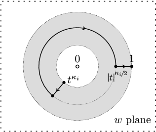
Figure A.1. The curve $\iota(t)$.

$$\iota(t)=\{(t^{\kappa_{i}}/\lambda,\lambda,t)\in\hat{H}_{\kappa_{i}}\,|\,t^{\kappa_{i}}\leq\lambda\leq 1\}.$$

For $t\in\mathbb{D}\setminus\mathbb{R}_{\leq 0}$ take the same definition for $\beta_{i}(t)$, now with $\iota(t)$ a continuous family of curves in $\hat{H}_{\kappa_{i}}$ in the fiber over $t$ that, projected to the $w$-plane, connects $t^{\kappa_{i}}$ and $1$ inside the annulus $|t^{\kappa_{i}}|\leq|w|\leq 1$.

For example, writing $t=|t|e^{\sqrt{-1}\theta}$ with $-\pi<\theta<\pi$, we could take $\iota(t):[0,1]\to\big{\{}w\in\mathbb{C}\,\big{|}\,|t|^{\kappa_{i}}\leq|w|\leq 1\}$ to map the three intervals (a) $[0,1/3]$, (b) $[1/3,2/3]$ and (c) $[2/3,1]$ to (a) the radial line segment connecting $t^{\kappa_{i}}=|t|^{\kappa_{i}}e^{\sqrt{-1}\theta}$ with $|t|^{\kappa_{i}/2}e^{\sqrt{-1}\theta}$, (b) an arc on a circle, with endpoint $|t|^{\kappa_{i}/2}$, (c) the radial line segment from $|t|^{\kappa_{i}/2}$ to $1$, respectively, and each interval parametrized with constant speed. Then indeed $\iota(t)$ varies continuously with $t\in\mathbb{C}\setminus\mathbb{R}_{\leq 0}$. Moreover, decomposing $\tilde{H}_{\kappa_{i}}\cap\big{(}\hat{\mathbb{D}}^{2}\times\{|t|\}\big{)}$ into two annuli of outer radius $1$ and inner radius $|t|^{1/2}$, we see that $\iota(t)$ for $t\to 0$ converges to the curve $\iota$ in (Cy II) of Construction A.3.

(C) For each $i$ with $\Phi_{i}$ of type I and each component $\gamma_{i}^{\mu}=-\gamma_{j}^{\nu}$ of $\partial\beta_{i}$ define the interpolating $p$-chain

$$\beta_{i,\mu}(t):={\Phi_{ij}}_{*}\big{(}[0,1]\times\gamma_{i}^{\mu}\times\{t\}\big{)}.$$

If also $\Phi_{j}$ is of type I we only consider $\beta_{i,\mu}$ if $i<j$.

Finally, define

$$\beta(t)=\sum_{i}\beta_{i}(t)+\sum_{i,\mu}\beta_{i,\mu}(t).$$

Note that $\beta(t)$ is a cycle since by construction: $\partial\beta_{i}(t)=\sum_{\mu}\gamma_{i}^{\mu}(t)$ with $\gamma_{i}^{\mu}(t)$ a continuous family of cycles converging to $\gamma_{i}^{\mu}$ for $t\to 0$, while by (C) it holds $\partial\beta_{i,\mu}(t)=-\gamma_{i}^{\mu}(t)-\gamma_{j}^{\nu}(t)$.

To finish the proof, it remains to compute $\int_{\beta(t)}\alpha$ and to match the various contributions with the terms in (A.9), modulo $t^{k+1}$. For contributions from (A) we have

$$\int_{\beta_{i}(t)}\alpha=\int_{\beta_{i}\times\{t\}}\Phi_{i}^{*}\alpha.$$

Developing the integrand in $t$ up to order $k$ yields $\int_{\beta_{i}}\Phi_{i}^{+}(\alpha)$.

For (B) and $t=|t|e^{\sqrt{-1}\theta}\neq 0$ we may eliminate $z=t^{\kappa_{i}}/w$ and work over the $w$-plane. The choice of $w$ over $z$ is motivated by the fact that the curve $\gamma_{i}$ moves radially inwards in the $z$-plane and outwards in the $w$-plane. In this coordinate, using $z^{r}dz=-t^{(r+1)\kappa_{i}}w^{-r-2}dw$ and following (A.4), (A.7), we can write uniquely

(A.11) $$\Phi_{i}^{*}\alpha=\sum_{r\geq 0}p_{\tilde{V}_{i}}^{*}h_{r}\wedge w^{r}dw+p_{\tilde{V}_{i}}^{*}h_{-1}\wedge\frac{dw}{w}-\sum_{r\geq 0}p_{\tilde{V}_{i}}^{*}g_{r}\wedge\frac{t^{(r+1)\kappa_{i}}}{w^{r+2}}dw+\alpha_{\tilde{V}_{i}},$$

with $h_{r},g_{r}\in\Gamma(V_{i}\times\mathbb{D},\Omega^{p-1}_{V_{i}\times\mathbb{D}/\mathbb{D}})$ and $\alpha_{\tilde{V}_{i}}\in\Gamma(\tilde{U}_{i},p_{V_{i}}^{*}\Omega^{p}_{V_{i}})$. Projected to the $w$-plane, $\iota(t)$ is a curve connecting $t^{\kappa_{i}}$ and $1$. If $\beta_{i}(t)=\gamma_{i}\times\Sigma(t)$, the integral over $\Phi_{i}^{*}\alpha$ involves integration of a holomorphic one-form over $\Sigma$ and hence it vanishes identically, in agreement with the first line in (A.8).

For the other case, $\beta_{i}(t)=\gamma_{i}\times\iota(t)$, we have

$$\int_{\iota(t)}w^{r}dw=\int_{t^{\kappa_{i}}}^{1}w^{r}dw=\begin{cases}\frac{1}{r+1}\big{(}1-t^{(r+1)\kappa_{i}}\big{)},&r\neq-1\\ -\kappa_{i}\log t,&r=-1.\end{cases}$$

Moreover, $\int_{\gamma_{i}\times\iota(t)}\alpha_{\tilde{V}_{i}}=0$ since $\alpha_{\tilde{V}_{i}}$ vanishes on $\operatorname{ker}({p_{\tilde{V}_{i}}}_{*})$. Integration of (A.11) over $\gamma_{i}\times\iota(t)$ now gives

$$\left(-\kappa_{i}\int_{\gamma_{i}}h_{-1}\right)\log t+\sum_{r\geq 0}\frac{1-t^{(r+1)\kappa_{i}}}{r+1}\left(\int_{\gamma_{i}}h_{r}-g_{r}\right).$$

Since $g_{r},h_{r}$ reduce modulo $t^{k+1}$ to the differential forms with the same symbols in Construction A.3 and since $g_{-1}=-h_{-1}=\operatorname{res}_{\Phi_{i}}(\alpha)$, this result agrees to order $k$ with the contributions to $\int_{\beta}\alpha$ in (A.9) from (A.8) and with $\kappa_{i}\big{(}\int_{\gamma_{i}}\operatorname{res}_{\Phi_{i}}(\alpha)\big{)}\log t$.

For the interpolation integrals (C) it holds

$$\int_{\beta_{i,\mu}(t)}\alpha=\int_{[0,1]\times\gamma_{i}^{\mu}\times\{t\}}\Phi_{ij}^{*}\alpha,$$

which agrees with $\int_{[0,1]\times\gamma_{i}^{\mu}}\Phi_{ij}^{+}(\alpha)$ in (A.9) upon reduction modulo $t^{k+1}$ by the same argument as in (A).

Any other choice of $\beta(t)$ differs from our choice up to homology by a sum of integrals over vanishing cycles of the form $\int_{{\Phi_{i}}_{*}(\gamma_{i}\times S^{1}\times\{t\})}\alpha$ for $\Phi_{i}$ of type II. Here $S^{1}\times\{t\}\subset\hat{H}_{\kappa_{i}}$ is defined by $|z|=|w|$. Integrating over the $S^{1}$-factor yields $2\pi\sqrt{-1}\int_{\gamma_{i}}\operatorname{res}_{\Phi_{i}}(\alpha)$, hence only changes the result as stated. ∎

Lemma A.7.

In the situation of Proposition A.6, let $T$ denote the monodromy transformation on $n$-cycle classes along a counter-clockwise simple loop in the base disk $\mathbb{D}$ of the family $\mathcal{X}\to\mathbb{D}$ based at a fiber $\mathcal{X}_{t_{0}}$ for some $t_{0}\neq 0$. We have

$$(T-\operatorname{id})(\beta_{t_{0}})=\sum\kappa_{i}[\gamma_{i}\times S^{1}]$$

where, in the notation of the proof of the proposition, the sum is over all charts of type (B) for which $\beta_{i}=\gamma_{i}\times\iota$ and $S^{1}$ denotes a clockwise simple loop around the origin in the $w$-plane, see Figure A.1.

Proof.

The cycle $\beta_{t_{0}}$ decomposes into chains $\beta_{i}$ according to cases (A),(B),(C) as in the proof of Proposition A.6. For (A) and (C), it is straightforward to see that $\beta_{i}$ is invariant under monodromy because the family is trivial here. Hence, $(T-\operatorname{id})$ only yields contributions for case (B). Note further that the factor $\gamma_{i}$ is also invariant under monodromy, so we only need to consider the local situation of the map $H_{\kappa_{i}}\to\mathbb{D}$ given by $zw=t^{\kappa_{i}}$. In the sub-situation where $\beta_{i}=\gamma_{i}\times\Sigma(t)$, we find that $\Sigma(t_{0})$ is the fundamental chain of the fiber of $H_{\kappa_{i}}\to\mathbb{D}$ which is also invariant under monodromy. Thus, only the situation $\beta_{i}=\gamma_{i}\times\iota$ contributes, as claimed in the assertion. Studying how $\iota$ changes when following a simple counter-clockwise $t_{0}$-based loop in $\mathbb{D}$, as illustrated in Figure A.1, we see that $\iota$ gets mapped to $\iota+\kappa_{i}[S^{1}]$ under $T$. Adding the invariant factor $\gamma_{i}$ yields the assertion. ∎

Appendix B Analytic approximation of proper formal families

Theorem B.1.

Let $R=\mathbb{C}\{t,z_{1},\ldots,z_{r}\}/(g_{1},\ldots,g_{s})$ be a convergent power series algebra, $(S,0)\subset(\mathbb{C}^{r+1},0)$ the corresponding germ of analytic space and $(\widetilde{S},0)$ the completion in the closed subspace defined by $t$. Let $\widetilde{\pi}:(\mathfrak{X},X_{0})\to(\widetilde{S},0)$ be a proper and flat formal analytic map and $\pi_{k}:X_{k}\to S_{k}$ its reduction modulo $t^{k+1}$.

Then for any $k\geq 0$ there exists a proper flat analytic map of germs of pairs $\pi:(\mathcal{X},X_{0})\to(S,0)$ with reduction modulo $t^{k+1}$ isomorphic to $\pi_{k}$.

Analogous approximation statements hold for morphisms of complex spaces $(\mathfrak{Z},Z_{0})\to(\mathfrak{X},X_{0})$, both of which proper and flat over $(\tilde{S},0)$, and for the additional giving of an $(\tilde{S},0)$-flat analytic subspace $(\mathfrak{D},D_{0})$ of $(\mathfrak{X},X_{0})$.

Proof.

We first treat the case $(\mathfrak{X}.X_{0})\to(\tilde{S},0)$. By a result of Douady and Grauert, the compact complex space $X_{0}$ admits a versal deformation, a proper analytic map $h:\mathcal{Y}\to V$ with a point $v\in V$ and an isomorphism $h^{-1}(v)\simeq X_{0}$ which is versal for proper flat analytic deformations of $X_{0}$ ([Du74], VII.8, Théorème Principal and [Gr], §5, Hauptsatz). Possibly by shrinking $V$, we may assume $V$ is an analytic subspace of an open subset in $\mathbb{C}^{n}$ given by some $f_{1},\ldots,f_{m}\in\mathbb{C}\{x_{1},\ldots,x_{n}\}$ and $v=0$. Thus for any given $k$ there exists a cartesian diagram of analytic spaces

(B.1)

We are going to construct $(\mathcal{X},X_{0})\to(S,0)$ by extending $\Phi_{k}$ to an analytic map $\Phi:(S,0)\to(V,0)$, first formally and then analytically using Artin approximation.

To do so, denote by $\widehat{\pi}:\widehat{\mathfrak{X}}\longrightarrow\widehat{S}$ and by $\widehat{h}:\widehat{\mathcal{Y}}\to\widehat{V}$ the completions of $\widetilde{\pi}$ and $h$ at the origins, respectively. By results of Schuster and Wavrik [St71], [Wa], the family $\widehat{h}$ is formally versal. Hence there exists a cartesian square

We can also achieve that the reduction of $\widehat{\Phi}$ modulo $t^{k+1}$ agrees with the completion $\widehat{\Phi}_{k}$ of $\Phi_{k}$ at $0$. Indeed, if $\mathfrak{m}\subset R$ is the maximal ideal, constructing $\widehat{\Phi}$ amounts to finding a compatible system of lifts

$$\widehat{\Phi}_{l}:\mathcal{O}_{\widehat{V},0}=\mathbb{C}\llbracket x_{1},\ldots,x_{n}\rrbracket/(f_{1},\ldots,f_{m})\longrightarrow R/\mathfrak{m}^{l+1},\quad l\in\mathbb{N},$$

along with a compatible system of isomorphisms of $X_{l}\to S_{l}$ with the pull-back of $\widehat{h}$ by $\widehat{\Phi}_{l}$. Assuming $\widehat{\Phi}_{l-1}$ given, the construction of $\widehat{\Phi}_{l}$ can be done in two steps: First provide the lift to

$$R/\big{(}\mathfrak{m}^{l+1}+(t^{k+1})\cap\mathfrak{m}^{l}\big{)}=R/\mathfrak{m}^{l}\times_{R/(\mathfrak{m}^{l}+(t^{k+1}))}R/\big{(}\mathfrak{m}^{l+1}+(t^{k+1})\big{)},$$

by gluing the family over $R/\mathfrak{m}^{l}$ given by $\widehat{\Phi}_{l-1}$ with the reduction modulo $\mathfrak{m}^{l+1}$ of $X_{k}/S_{k}$, using the given isomorphism of the common reductions modulo $\mathfrak{m}^{l}+(t^{k+1})$. The fibered sum of analytic spaces involved in this step exists due to [St70], Satz 2.7. Then in the second step use formal versality to extend from $R/\big{(}\mathfrak{m}^{l+1}+(t^{k+1})\cap\mathfrak{m}^{l}\big{)}$ to $R/\mathfrak{m}^{l+1}$. Thus $\widehat{\Phi}$ with the requested properties exists.

Writing $\mathbf{z}=(z_{1},\ldots,z_{r})$, the map $\widehat{\Phi}$ is given by equations $x_{i}=\widehat{\varphi}_{i}(t,\mathbf{z})$ for $1\leq i\leq n$ with $\widehat{\varphi}_{i}\in\mathbb{C}\llbracket t,\mathbf{z}\rrbracket$. Since the ideal $(f_{1},\ldots,f_{m})$ gets mapped into the ideal $(g_{1},\ldots,g_{s})$, the $\widehat{\varphi}_{i}$ fulfill the system of equations

(B.2) $$f_{j}\big{(}\widehat{\varphi}_{1}(t,\mathbf{z}),\ldots,\widehat{\varphi}_{n}(t,\mathbf{z})\big{)}=\sum_{\sigma=1}^{s}\widehat{a}_{j\sigma}(t,\mathbf{z})g_{\sigma}(t,\mathbf{z}),\quad 1\leq j\leq m$$

for some $\widehat{a}_{j\sigma}\in\mathbb{C}\llbracket{t,\bf z}\rrbracket$. Since we already have the analytic solution $\Phi_{k}$ on $S_{k}$, that is, an analytic solution modulo $t^{k+1}$, we now rewrite

$$\widehat{\varphi}_{i}=\varphi_{i}+t^{k+1}\widehat{\psi}_{i},\quad i=1,\ldots,m,$$

with $\varphi_{i}\in\mathbb{C}\{t,\mathbf{z}\}$ the components of $\Phi_{k}$ and $\widehat{\psi}_{i}\in\mathbb{C}\llbracket t,\mathbf{z}\rrbracket$. Plugging into (B.2) we see that $y_{i}=\widehat{\psi}_{i}(t,\mathbf{z})$, $x_{j\sigma}=\widehat{a}_{j\sigma}(t,\mathbf{z})$ are a formal solution of the system of analytic equations

(B.3) $$f_{j}\big{(}\varphi_{1}(t,\mathbf{z})+t^{k+1}y_{1},\ldots,\varphi_{n}(t,\mathbf{z})+t^{k+1}y_{n}\big{)}=\sum_{\sigma=1}^{s}x_{j\sigma}g_{\sigma}(t,\mathbf{z}),\quad 1\leq j\leq m.$$

By Artin’s approximation theorem [At], Theorem 1.2, there exist germs of analytic functions $\psi_{1}(t,\mathbf{z}),\ldots,\psi_{n}(t,\mathbf{z})$ and $a_{j\sigma}(t,\mathbf{z})$ that solve (B.3). Now $\varphi_{1}+t^{k+1}\psi_{1},\ldots,\varphi_{n}+t^{k+1}\psi_{n}$ defines an analytic map $(S,0)\to(V,0)$ with the property that the reduction modulo $t^{k+1}$ equals $\Phi_{k}$. The base change $\mathcal{X}:=\mathcal{Y}\times_{V}S$ of $\mathcal{Y}\to V$ by $\Phi$ is the requested analytic approximation of $\widetilde{\pi}$. This finishes the proof for the case $(\mathfrak{X},X_{0})\to(\tilde{S},0)$.

The proof for the case of a morphism $(\mathfrak{Z},Z_{0})\to(\mathfrak{X},X_{0})$ is similar, replacing the versal deformation of $X_{0}$ by the versal deformation of the morphism $Z_{0}\to X_{0}$, with varying domain and target. This latter versal deformation space exists by first constructing versal deformations $\mathcal{T}\to W$ of $Y_{0}$ and $\mathcal{Y}\to V$ of $X_{0}$ separately, and then taking the relative hom space $\operatorname{Hom}_{W\times V}(\mathcal{T}\times V,W\times\mathcal{Y})$ from [Du69], Ch.10, for the pull-backs to $W\times V$ of the versal deformations of domain and target. The case of an analytic subspace is a special case, noting that the condition that a morphism is a closed embedding is an open property. ∎

Appendix C The divisorial log deformation functor has a hull

In this section, $X_{\mathbb{C}}$ denotes a simple toric log Calabi-Yau space over $(\operatorname{Spec}\mathbb{C},\mathbb{N}\times\mathbb{C}^{\times})$. We consider divisorial deformations of $X_{\mathbb{C}}$ as defined in [GS2], Definition 2.7. Let $\mathcal{D}:(\hbox{Artinian $\mathbb{C}\llbracket t\rrbracket$-algebras})\to(\hbox{Sets})$ be the divisorial log deformation functor hence that associates to an Artinian $\mathbb{C}\llbracket t\rrbracket$-algebra $A$ the set of isomorphism classes of divisorial log deformations $X_{A}$ of $X_{\mathbb{C}}$ over $\operatorname{Spec}A$ equipped with the divisorial log structure defined by $t=0$. The definition requires $X_{A}\to\operatorname{Spec}A$ to be flat in the ordinary sense, to be log smooth away from $Z$ and to permit local models of a particular type along $Z$. The last condition requires that each $\bar{x}\in Z$ has an étale neighborhood $V_{A}$ with strict étale $\operatorname{Spec}A$-morphisms $X_{A}\leftarrow V_{A}\to Y_{A}=\operatorname{Spec}A\times_{\mathbb{C}\llbracket t\rrbracket}U$ where $U\to\operatorname{Spec}\mathbb{C}\llbracket t\rrbracket$ is a particular affine toric variety with monomial function $t$ uniquely determined by $\bar{x}$. In the following we call such an étale neighborhood $V_{A}\to X_{A}$ a model neighborhood. The only feature of these local models needed for the present discussion is the following result from [GS10].

Lemma C.1.

([GS10], Lemma 2.15.) For every $\bar{x}\in Z$, there exists a model neighborhood $V_{\mathbb{C}}$ of $\bar{x}$ in $X_{\mathbb{C}}$, so that for every Artinian $\mathbb{C}\llbracket t\rrbracket$-algebra $A$, any two divisorial log deformations of $V_{\mathbb{C}}$ over $\operatorname{Spec}A$ are isomorphic.

A standard fact about étale maps (Remark 2.4 in [GS10]) is the following:

Lemma C.2.

If $Y$ is a log scheme and $Y_{0}\subset Y$ a closed subscheme defined by a nilpotent sheaf of ideals with restriction of the log structure from $Y$, then the category of strict étale $Y$-schemes is equivalent to the category of strict étale $Y_{0}$-schemes by means of $V\mapsto V\times_{Y}Y_{0}$.

Lemma C.3.

Assume that $A_{1}\to A_{0}\leftarrow A_{2}$ are maps of Artinian $\mathbb{C}\llbracket t\rrbracket$-algebras and $X_{A_{1}}\leftarrow X_{A_{0}}\to X_{A_{2}}$ maps of divisorial log deformations above these. Given $\bar{x}\in Z$, there is the following commutative diagram with all squares cartesian, rows local models at $\bar{x}$, left column the given maps of deformation and the right column the maps induced via pullback by $U\to\operatorname{Spec}\mathbb{C}\llbracket t\rrbracket$,

Proof.

Let $X_{\mathbb{C}}\leftarrow V_{\mathbb{C}}\to Y_{\mathbb{C}}$ be a model neighborhood of $\bar{x}\in Z$ in $X_{\mathbb{C}}$ provided by Lemma C.1. Then Lemma C.2 implies that for any Artinian $\mathbb{C}\llbracket t\rrbracket$-algebra $A$ and divisorial log deformation $X_{A}\in\mathcal{D}(A)$ of $X_{\mathbb{C}}$, there exists a model neighborhood $X_{A}\leftarrow V_{A}\to Y_{A}$ restricting to $X_{\mathbb{C}}\leftarrow V_{\mathbb{C}}\to Y_{\mathbb{C}}$. Moreover, this model neighborhood is unique up to unique isomorphism. Thus the extension of the given model neighborhood $X_{\mathbb{C}}\leftarrow V_{\mathbb{C}}\to Y_{\mathbb{C}}$ to divisorial log deformations of $X_{\mathbb{C}}$ is functorial, which in particular gives the stated commutative diagram. ∎

An important fact implied from the definition is that the log structure on $X_{A}$ has integral stalks even though it typically is not coherent. Recall that a morphism $f:(X,\mathcal{M}_{X})\to(Y,\mathcal{M}_{Y})$ of log spaces with integral monoid stalks is strict if and only the induced map $f^{-1}\overline{\mathcal{M}}_{Y}\to\overline{\mathcal{M}}_{X}$ is an isomorphism.

Lemma C.4.

If $f:X_{A}\to X_{A^{\prime}}$ is a map of divisorial log deformations over a homomorphism of Artinian $\mathbb{C}\llbracket t\rrbracket$-algebras, then $f$ is strict.

Proof.

By strictness of $X_{\mathbb{C}}\to X_{A}$, $X_{\mathbb{C}}\to X_{A^{\prime}}$, the map $f^{-1}\overline{\mathcal{M}}_{X_{A^{\prime}}}\to\overline{\mathcal{M}}_{X_{A}}$ induced by $f$ is an isomorphism. The statement now follows by integrality of stalks. ∎

Lemma C.5.

Assume we have a commutative diagram of Noetherian rings

$$\begin{CD}B_{1}@>{}>{}>B_{0}@<{b}<{}<B_{2}\\ @V{}V{}V@V{}V{}V@V{}V{}V\\ C_{1}@>{}>{}>C_{0}@<{c}<{}<C_{2}\end{CD}$$

with $b,c$ surjective with nilpotent kernel, the squares co-cartesian and all vertical maps flat and unramified, then the natural map $f:B_{1}\times_{B_{0}}B_{2}\to C_{1}\times_{C_{0}}C_{2}$ is also flat and unramified.

Proof.

The question is local, so we can assume all rings local and $B_{i}\to C_{i}$ are standard, that is, $C_{i}=B_{i}[T]/(P_{i})$ for $P_{i}\in B_{i}[T]$ monic with simple roots. By co-cartesianness, we may assume $P_{0}$ is the image of $P_{1},P_{2}$ under $B_{i}[T]\to B_{0}[T]$. Thus $P_{1},P_{2}$ define a polynomial $P\in(B_{1}\times_{B_{0}}B_{2})[T]$, which is clearly monic. Moreover, $P$ also has simple roots because any double root would imply a double root also for all the other $P_{i}$ using that $\operatorname{Spec}(B_{1}\times_{B_{0}}B_{2})\to\operatorname{Spec}B_{1}$ is bijective by surjectivity of $b:B_{2}\to B_{0}$. Finally, we find that $C_{1}\times_{C_{0}}C_{2}=(B_{1}\times_{B_{0}}B_{2})[T]/(P)$, which implies the assertion. ∎

Let $A_{1}\to A_{0}\leftarrow A_{2}$ be homomorphisms of Artinian $\mathbb{C}\llbracket t\rrbracket$-algebras. Consider the natural map

(C.1) $$\mathcal{D}(A_{1}\times_{A_{0}}A_{2})\longrightarrow\mathcal{D}(A_{1})\times_{\mathcal{D}(A_{0})}\mathcal{D}(A_{2}).$$

The Schlessinger criteria that provide a hull are the following ([Sl], Theorem 2.11).

• The map (C.1) is surjective whenever $A_{2}\to A_{0}$ is surjective.

• The map (C.1) is bijective whenever $A_{0}=\mathbb{C}$ and $A_{2}=\mathbb{C}[\varepsilon]:=\mathbb{C}[E]/E^{2}$.

• $\dim_{k}(t_{\mathcal{D}})<\infty$ where $t_{\mathcal{D}}:=\mathcal{D}(\mathbb{C}[\varepsilon])$.

Theorem C.6.

The divisorial log deformation functor $\mathcal{D}$ has a hull.

Proof.

The last criterion (H3) is proved in [GS10], Theorem 2.11,(2). It remains to verify (H1) and (H2). We begin with (H1). Let $A_{2}\to A_{0}$ be surjective. Set $A:=A_{1}\times_{A_{0}}A_{2}$ and note this is naturally an Artinian $\mathbb{C}\llbracket t\rrbracket$-algebra. Let $(X_{i},\mathcal{M}_{i})\to\operatorname{Spec}{A_{i}}$ be divisorial log deformations lifting the maps $A_{0}\to A_{i}$. Just as in the proof of (H1) for the log smooth deformation functor in [Kf], we obtain a glued log space $(X_{A},\mathcal{N})$ via $\mathcal{N}:=\mathcal{M}_{1}\times_{\mathcal{M}_{0}}\mathcal{M}_{2}\to\mathcal{O}_{X_{1}}\times_{\mathcal{O}_{X_{0}}}\mathcal{O}_{X_{2}}=:\mathcal{O}_{X_{A}}$ with log map to $(\operatorname{Spec}A,\mathbb{N}\times A^{\times})$ compatible with restrictions to $X_{0},X_{1},X_{2}$. In view of Lemma C.4, we have $\overline{\mathcal{M}}_{1}=\overline{\mathcal{M}}_{0}=\overline{\mathcal{M}}_{2}=:\overline{\mathcal{M}}$ and there is a natural map $\alpha:\overline{\mathcal{N}}\to\overline{\mathcal{M}}_{1}\times_{\overline{\mathcal{M}}_{0}}\overline{\mathcal{M}}_{2}=\overline{\mathcal{M}}$ that we claim is an isomorphism. Indeed, since $\overline{\mathcal{M}}_{2}\to\overline{\mathcal{M}}_{0}$ is surjective, $\alpha$ is easily seen to be surjective. Now assume $(m_{1},m_{2}),(m_{1}^{\prime},m_{2}^{\prime})\in\overline{\mathcal{N}}$ map to the same element under $\alpha$. Then $m_{1}=\varepsilon_{1}m_{1}^{\prime},m_{2}=\varepsilon_{2}m_{2}^{\prime}$ for $\varepsilon_{i}\in\mathcal{M}_{i}^{\times}$. The cancellation law in $\mathcal{M}_{0}$ gives that $\varepsilon_{1}$ and $\varepsilon_{2}$ map to the same element in $\mathcal{M}_{0}^{\times}$, hence glue to an element of $\mathcal{N}^{\times}$. Thus $(m_{1},m_{2})$ and $(m_{1}^{\prime},m_{2}^{\prime})$ map to the same element in $\overline{\mathcal{N}}$, proving injectivity of $\alpha$. By the same argument as in Lemma C.4, we now know that $X_{i}\to X_{A}$ are strict.

Away from the incoherent locus $Z$, it was argued in [Kf] that $(X_{A},\mathcal{N})$ is a log smooth lifting of $X_{0}$. It remains to show the existence of local models along $Z$ (which then also implies the flatness along $Z$). Let $\bar{x}\in Z$ be a geometric point. Lemma C.3 provides a diagram of local models and we use the push-out for each row to obtain the following commutative diagram

The dashed maps are étale by Lemma C.5 and $Y_{A}$ agrees with $\operatorname{Spec}A\times_{\operatorname{Spec}\mathbb{C}\llbracket t\rrbracket}U$. The strictness of all vertical maps follows from the strictness of $X_{i}\to X_{A}$ proved above. Lemma C.4 then also gives strictness of the dashed maps, using that $X_{1}\to X_{A}$ is a homeomorphism on underlying spaces. We now have obtained local models for $X_{A}$, so $X_{A}$ is a divisorial log deformation of $X_{\mathbb{C}}$ that maps to $(X_{1},X_{2})$ under the map in (C.1). Thus this map is surjective, finishing the proof of (H1).

Finally we turn to (H2), for which only injectivity is left to be shown. Let $A_{0}=\mathbb{C}$ and $A_{2}=\mathbb{C}[\varepsilon]$. Using the same reasoning as in [Kf], Proof of (H2), it suffices to prove the following assertion (Lemma 9.2 in [Kf]).

If $(X_{A}^{\prime},\mathcal{N}^{\prime})\to(\operatorname{Spec}A_{i},\mathbb{N}\times A_{i}^{\times})$ is a divisorial log deformation that fits in a commutative square

$$\begin{CD}(X_{1},\mathcal{M}_{1})@>{}>{}>(X_{A}^{\prime},\mathcal{N}^{\prime})\\ @A{}A{}A@A{}A{}A\\ (X_{0},\mathcal{M}_{0})@>{}>{}>(X_{2},\mathcal{M}_{2})\end{CD}$$

so that the restriction maps to $(X_{i},\mathcal{M}_{i})$ for $i=1,2$ induce isomorphisms, then the natural map $f:(X_{A},\mathcal{N})\to(X_{A}^{\prime},\mathcal{N}^{\prime})$ is an isomorphism. The proof in [Kf] works for us away from $Z$, so it remains to prove $f$ is an isomorphism along $Z$. Let $\bar{x}\in Z$ be a point and let $V^{\prime}_{A}\to X_{A}^{\prime}$ be the strict étale neighborhood of $\bar{x}$ obtained from the neighborhood $V_{\mathbb{C}}$ of $\bar{x}$ in $X_{\mathbb{C}}$ via Lemma C.2. Then Lemma C.1 provides a $\operatorname{Spec}A$-isomorphism $V^{\prime}_{A}\stackrel{{\scriptstyle\sim}}{{\to}}V_{A}$. Since the restrictions to $X_{\mathbb{C}}\leftarrow V_{\mathbb{C}}$ are compatible isomorphisms, Lemma C.2 shows this isomorphism commutes with $f$. In particular, $f$ is an isomorphism at $\bar{x}$, completing the proof. ∎

Appendix D Isomorphism of affine and algebraic $H^{1}(\Theta)$

Let $(B,\mathscr{P},\varphi)$ be a simple tropical manifold and $x\in\operatorname{Spec}(\mathbb{C}[H^{1}(B,i_{*}\check{\Lambda})^{*}])$ a closed point. Let $X_{x}$ denote the fiber of the canonical family above it. In particular $(B,\mathscr{P})$ is the intersection complex of $X_{0}(B,\mathscr{P})$ and also of $X_{x}$. Occurrences of $\tau,\sigma$ with various indices below will always refer to cells in $\mathscr{P}$. Inclusions of closed strata are covariant: $\tau_{0}\subset\tau_{1}\Rightarrow X_{\tau_{0}}\subset X_{\tau_{1}}$. Note that, inconveniently, in order to parse all upcoming references to [GS10], a mental translation to the dual intersection complex as used in [GS10] must be made. The translation is straightforward, but nonetheless potentially confusing. For $\sigma\in\mathscr{P}$, let $V_{\sigma}$ denote the standard open set of $X_{x}$ that is the open star of the dense torus of the stratum $X_{\sigma}$, i.e. the disjoint union of the dense torus orbits of all $X_{\sigma^{\prime}}$ for $\sigma^{\prime}$ containing $\sigma$. Note the contravariance: $V_{\sigma_{1}}\subset V_{\sigma_{0}}$ for ${\sigma_{0}}\subset{\sigma_{1}}$. Refine the partial order $\subseteq$ of $\mathscr{P}$ to a total order $\leq$ so that for any sheaf $\mathcal{F}$ on $X_{x}$ we obtain a Čech complex $\check{C}^{j}(\{V_{\sigma}\}_{\sigma},\mathcal{F})=\bigoplus_{\sigma_{0}<\ldots<\sigma_{j}}\Gamma(V_{\sigma_{0}}\cap\ldots\cap V_{\sigma_{j}},\mathcal{F})$ with the usual Čech differential $\check{C}^{j}\to\check{C}^{j+1}$. A decoration with $\dagger$ refers to the space with log structure (given by $t=0$). Following [GS10], let $j:X_{x}\setminus Z_{x}\hookrightarrow X_{x}$ denote the open inclusion of the locus where the log structure is coherent and then we write short

$$\Omega^{r}:=j_{*}\Omega^{r}_{X_{x}^{\dagger}/x^{\dagger}},\qquad\Theta:=j_{*}\Theta_{X_{x}^{\dagger}/x^{\dagger}}.$$

The main purpose of this section is to prove the following proposition. For the statement, recall that $W_{\tau}\subset B$ denotes the open set given by the disjoint union of the relative interiors of all cells in the barycentric subdivision of $\mathscr{P}$ that contain the barycenter of $\tau$.

Proposition D.1.

We have a natural isomorphism of Čech cohomologies

$$\textstyle H^{1}\big{(}(W_{\tau})_{\tau},\iota_{*}\bigwedge^{n-1}\Lambda\otimes\mathbb{C}\big{)}\longrightarrow\check{H}^{1}(\{V_{\tau}\}_{\tau},\Omega^{n-1}).$$

Moreover, if $B$ is orientable, using the global volume forms $\iota_{*}\bigwedge^{n}\Lambda\simeq\underline{\mathbb{Z}}$ and $\Omega^{n}\simeq\mathcal{O}_{X_{x}}$, this isomorphism can be rewritten as

$$\check{H}^{1}\big{(}(W_{\tau})_{\tau},\iota_{*}\check{\Lambda}\otimes\mathbb{C}\big{)}\longrightarrow\check{H}^{1}(\{V_{\tau}\}_{\tau},\Theta).$$

Explicitly, the image of a cocycle $\big{(}n_{\omega\tau}\big{)}_{\omega,\tau}$ with $n_{\omega\tau}\in\Gamma(W_{\omega}\cap W_{\tau},\iota_{*}\check{\Lambda}\otimes\mathbb{C})$ is the cocycle $\big{(}\partial_{n_{\omega\tau}}\big{)}_{\omega\tau}$ with $\partial_{n_{\omega\tau}}\in\Gamma(V_{\omega}\cap V_{\tau},\Theta)$ the logarithmic vector field defined by $n_{\omega\tau}$.

For $\tau_{0}\subseteq\tau_{1}$, recall from [GS10], Lemma 3.20, the isomorphism

(D.1) $$\textstyle\Gamma(W_{\tau_{0}}\cap W_{\tau_{1}},\iota_{*}\bigwedge^{r}\Lambda\otimes\mathbb{C})=\Gamma(X_{\tau_{0}},(\Omega^{r}_{\tau_{1}}|_{X_{\tau_{0}}})/{\mathcal{T}ors})$$

where $\Omega^{r}_{\tau}=\kappa_{\tau,*}\kappa_{\tau}^{*}(\Omega^{r}|_{X_{\tau}})$ for $\kappa_{\tau}:X_{\tau}\setminus Z_{\tau}\hookrightarrow X_{\tau}$ the open embedding defined in loc.cit.. Note that, by the argument in the proof of Theorem 3.21 of [GS10], we have

(D.2) $$\textstyle\Gamma(W_{\tau_{0}}\cap\ldots\cap W_{\tau_{i}},\iota_{*}\bigwedge^{r}\Lambda\otimes\mathbb{C})=\Gamma(W_{\tau_{0}}\cap W_{\tau_{i}},\iota_{*}\bigwedge^{r}\Lambda\otimes\mathbb{C}).$$

We will use this identification to define a map of double complexes ${\bf\Lambda}^{i,j}\to{\bf\Omega}^{i,j}$ and we only care about $r=n-1$ for $n=\dim B$. The first of these double complexes arises as a “doubling” of the Čech complex of $\iota_{*}\bigwedge^{n-1}\Lambda$ with respect to the cover $\{W_{\tau}\}_{\tau\in\mathscr{P}}$, as follows:

(D.3) $$\textstyle{\bf\Lambda}^{i,j}=\bigoplus_{\sigma_{0}\subsetneq\ldots\subsetneq\sigma_{j}\subseteq\tau_{0}\subsetneq\ldots\subsetneq\tau_{i}}\Gamma((W_{\tau_{0}}\cap W_{\tau_{i}})\cap(W_{\sigma_{0}}\cap W_{\sigma_{j}}),\iota_{*}\bigwedge^{n-1}\Lambda\otimes\mathbb{C}).$$

Note that $W_{\sigma_{1}}\cap W_{\sigma_{2}}=\emptyset$ unless $\sigma_{1}\subseteq\sigma_{2}$ or $\sigma_{2}\subseteq\sigma_{1}$, so summing over $\sigma_{0}\subsetneq\ldots\subsetneq\sigma_{j}$ gives the Čech complex for the cover $\{W_{\tau}\}_{\tau}$:

$$\textstyle\bigoplus_{j=0}^{n}\Lambda^{i,j}=\check{C}^{i}\big{(}(W_{\tau})_{\tau},\iota_{*}\bigwedge^{n-1}\Lambda\otimes\mathbb{C}\big{)}.$$

Using (D.2), the differential $i\to i+1$ is the usual alternating sum of the Čech-differential, and similarly for the differential $j\to j+1$.

The second double complex is

(D.4) $${\bf\Omega}^{i,j}=\bigoplus_{\sigma_{0}\subsetneq\ldots\subsetneq\sigma_{j}\subseteq\tau_{0}\subsetneq\ldots\subsetneq\tau_{i}}\Gamma(X_{\tau_{0}}\cap V_{\sigma_{0}}\cap\ldots\cap V_{\sigma_{j}},(\Omega^{n-1}_{\tau_{i}}|_{X_{\tau_{0}}\cap V_{\sigma_{j}}})/{\mathcal{T}ors}).$$

The differential $i\to i+1$ is the differential $d_{\operatorname{bct}}$ given in [GS10], p.736, just before Theorem 3.9 and the differential $j\to j+1$ is a Čech-type-differential analogous to the one in ${\bf\Lambda}^{i,j}$. Note however that, unlike for the cover $\{W_{\sigma}\}_{\sigma}$, we may have $V_{\sigma_{1}}\cap V_{\sigma_{2}}\neq\emptyset$ even if none of $\sigma_{1},\sigma_{2}$ is contained in the other. We will later use Lemma D.4 to take care of this fact.

Lemma D.2.

There is a natural injection of double-complexes $\Phi:{\bf\Lambda}^{i,j}\to{\bf\Omega}^{i,j}$.

Proof.

Given $\sigma_{0}\subseteq\ldots\subseteq\sigma_{j}\subseteq\tau_{0}$, the torus-invariant open subset $X_{\tau_{0}}\cap V_{\sigma_{0}}\cap\ldots\cap V_{\sigma_{j}}=X_{\tau_{0}}\cap V_{\sigma_{j}}$ of the toric variety $X_{\tau_{0}}$ is of the form $V=\operatorname{Spec}\mathbb{C}[P]$ for $P$ a toric monoid. By [GS10], Lemma 3.12 and Proposition 3.17, there is an injection $\Omega^{r}_{\tau}\hookrightarrow\Omega^{r}_{X_{\hat{\tau}}}(\log\partial X_{\hat{\tau}})|_{X_{\tau}}=\mathcal{O}_{X_{\tau}}\otimes_{\mathbb{Z}}\bigwedge^{r}\Lambda_{\hat{\tau}}$ for any maximal cell $\hat{\tau}$ containing $\tau$. Here, $1\otimes(m_{1}\wedge\ldots\wedge m_{r})$ gets identified with $\frac{dz^{m_{1}}}{z^{m_{1}}}\wedge\ldots\wedge\frac{dz^{m_{r}}}{z^{m_{r}}}$. When changing the choice of $\hat{\tau}$, identifying $\Lambda_{\hat{\tau}}$ with another $\Lambda_{\hat{\tau}^{\prime}}$ generally depends on the chosen path in $B\setminus\Delta$, and furthermore the gluing data rescale the monomials. Both of these won’t bother us for the following reasons. We will only be interested in the subsheaf $\mathbb{C}\otimes_{\mathbb{Z}}\bigwedge^{r}\Lambda_{\hat{\tau}}$ which is actually invariant under this torus action, because the scaling operation $z\mapsto\lambda z$ leaves $\frac{dz}{z}$ invariant. Even better, we will actually only care about the monodromy invariant part of this subsheaf. With this in mind, in view of (D.3), it is straightforward to produce the following map

$$\textstyle\Gamma((W_{\tau_{0}}\cap W_{\tau_{i}})\cap(W_{\sigma_{0}}\cap W_{\sigma_{j}}),\iota_{*}\bigwedge^{n-1}\Lambda\otimes\mathbb{C}) \stackrel{{\scriptstyle\eqref{only-outer-ones-matter}}}{{=}}\textstyle\mathbb{C}\otimes\Gamma(W_{\sigma_{0}}\cap W_{\tau_{i}},\iota_{*}\bigwedge^{n-1}\Lambda)$$

$$\hookrightarrow\Gamma(X_{\tau_{0}}\cap V_{\sigma_{j}},(\Omega^{n-1}_{\hat{\tau}}|_{X_{\tau_{0}}\cap V_{\sigma_{j}}})/{\mathcal{T}ors})$$

and its image is contained in $\Gamma(X_{\tau_{0}}\cap V_{\sigma_{j}},(\Omega^{n-1}_{\tau_{i}}|_{X_{\tau_{0}}\cap V_{\sigma_{j}}})/{\mathcal{T}ors})$. This gives an injection from the sum in (D.3) to the one in (D.4). The map respects the differentials by what we said before and by the functoriality of Čech-type complexes. ∎

Remark D.3.

We never used that $r=n-1$, so a similar map as in the previous lemma exists for any $r$. In fact, the statement of Lemma D.2 can be upgraded to an injection of triple complexes when taking the de Rham differential for ${\bf\Omega}^{i,j}$ and an additional trivial differential $r\to r+1$ on ${\bf\Lambda}^{i,j}$.

We need a technical lemma before we can prove Proposition D.1. For a sheaf $\mathcal{F}$ on $X_{x}$, consider the exact sequence of complexes

Lemma D.4.

The surjection $e$ is a quasi-isomorphism. Denoting by $d_{2}$ the differential in the second index of ${\bf\Omega}^{i,j}$, we conclude that

(D.5) $$H^{p}_{d_{2}}({\bf\Omega}^{i,\bullet})=\bigoplus_{\tau_{0}\subsetneq\ldots\subsetneq\tau_{i}}H^{p}(X_{\tau_{0}},(\Omega^{n-1}_{\tau_{i}}|_{X_{\tau_{0}}})/{\mathcal{T}ors}).$$

Proof.

We show that $K^{\bullet}$ is acyclic. Note that $V_{\sigma_{0}}\cap\ldots\cap V_{\sigma_{j}}=\emptyset$ unless there is a $\sigma\in\mathscr{P}$ that contains $\sigma_{0},\ldots,\sigma_{j}$. Let $\langle\sigma_{0},\ldots,\sigma_{j}\rangle$ denote the set of minimal elements with respect to $\subseteq$ in the set of all $\sigma\in\mathscr{P}$ that contain $\sigma_{0},\ldots,\sigma_{j}$ (e.g. for $(B,\mathscr{P})$ two intervals glued to form a circle and $\sigma_{0},\sigma_{1}$ being the two vertices, we have $\langle\sigma_{0},\sigma_{1}\rangle$ is the set containing the two intervals). The use of this definition is the following observation

$$V_{\sigma_{0}}\cap\ldots.\cap V_{\sigma_{j}}=\bigsqcup_{\sigma\in\langle\sigma_{0},\ldots,\sigma_{j}\rangle}V_{\sigma}.$$

Let $K_{\sigma}^{\bullet}$ be the subcomplex of $K^{\bullet}$ consisting of the summands for open sets contained in $V_{\sigma}$, in particular involving only summands of terms for $\sigma_{0}<\ldots<\sigma_{j}$ where $\sigma$ contains $\sigma_{0},\ldots,\sigma_{j}$. The subcomplexes $K_{i}^{\bullet}=\sum_{\dim\sigma=i}K_{\sigma}^{\bullet}$ form a filtration of $K^{\bullet}$. We show that the gradeds of this filtration are acyclic. Let $\bar{K}_{\sigma}^{\bullet}$ be the quotient of $K_{\sigma}^{\bullet}$ defined by removing terms where $V_{\sigma}$ is properly contained in a component of $V_{\sigma_{0}}\cap\ldots\cap V_{\sigma_{j}}$ rather than equal to a component, precisely

$$\bar{K}_{\sigma}^{j}=\bigoplus_{{\sigma_{0}<\ldots<\sigma_{j}}\atop{\sigma\in\langle\sigma_{0},\ldots,\sigma_{j}\rangle}}\Gamma(V_{\sigma},\mathcal{F}).$$

We have $K_{i}/K_{i+1}=\bigoplus_{\dim\sigma=i}\bar{K}_{\sigma}^{\bullet}$. We find that $\bar{K}_{\sigma}^{\bullet}$ is isomorphic to the cone of an isomorphism of complexes and thus acyclic. Indeed, write $\bar{K}_{\sigma}^{\bullet}={}_{1}\bar{K}_{\sigma}^{\bullet}\to{}_{2}\bar{K}_{\sigma}^{\bullet}$ where ${}_{1}\bar{K}_{\sigma}^{\bullet}$ gathers the summands with $\sigma_{j}\neq\sigma$ and ${}_{2}\bar{K}_{\sigma}^{\bullet}$ gathers the summands with $\sigma_{j}=\sigma$. We finished showing the acyclicity of $K^{\bullet}$.

Since $V_{\sigma}$ is affine for each $\sigma$ and so are their intersections, $\{V_{\sigma}\}_{\sigma}$ forms an affine cover of $X_{x}$. Let $q_{\tau}:X_{\tau}\to X_{x}$ denote the inclusion of the stratum. We have for $\mathcal{F}:=q_{\tau,*}(\Omega^{n-1}_{\tau_{i}}|_{X_{\tau_{0}}})/{\mathcal{T}ors}$ that the quasi-isomorphism $e$ is a map between the Čech complex of $\mathcal{F}$ and a summand of the complex $({\bf\Omega}^{i,\bullet},d_{2})$. Summing the maps $e$ for all these summands and taking cohomology yields (D.5). ∎

Proof of Proposition D.1.

The main tool is the injection of double complexes $\Phi$ from Lemma D.2. We consider taking cohomology for the second differential $j\to j+1$ for both complexes ${\bf\Lambda}^{i,j}$ and ${\bf\Omega}^{i,j}$. Lemma D.4 gives the result for the complex ${\bf\Omega}^{i,j}$. By the proof of Theorem 3.22 and Lemma 3.20 in [GS10], using that $r=n-1$, we find that $H^{p}_{d_{2}}({\bf\Omega}^{i,\bullet})=0$ for $p>0$. Note that this fails in general for other degrees $r$ as was found in [Ru10], Theorem 1.6. We also have that $H^{p}_{d_{2}}({\bf\Lambda}^{i,\bullet})=0$ for $p>0$ since the cover $\{W_{\tau}\}_{\tau}$ is acyclic for $\iota_{*}\bigwedge^{r}\Lambda$ for any $r$ by [GS06], Lemma 5.5. Thus, taking cohomology by the differential $j\to j+1$ on source and target of $\Phi$ simultaneously yields a map induced by $\Phi$ that is concentrated in degrees $(i,0)$. The resulting complexes for the remaining differential $i\to i+1$ the isomorphism of barycentric complexes that led to the proof of [GS10], Theorem 3.22. Consequently and relevant for us is the conclusion that $\Phi:{\bf\Lambda}^{i,j}\to{\bf\Omega}^{i,j}$ is a quasi-isomorphism on the total complex of the double complex.

We next consider what happens when we first take cohomology under the first differential $d_{1}$, that is, $i\to i+1$. All cohomology groups at $i>0$ vanish: for ${\bf\Lambda}^{i,j}$ again because of the acyclicity of the cover $\{W_{\tau}\}_{\tau}$ and for ${\bf\Omega}^{i,j}$ by the exactness of the barycentric differentials [GS06], Proposition A.2 and [GS10], Theorem 3.5.

Therefore, since $\Phi$ is a quasi-isomorphism, also the induced map on $d_{1}$-cohomology that is concentrated in $i=0$,

(D.6) $$\textstyle\tilde{\Phi}:\bigoplus_{\sigma_{0}\subsetneq\ldots\subsetneq\sigma_{j}}\Gamma(W_{\sigma_{0}}\cap W_{\sigma_{j}},\iota_{*}\bigwedge^{n-1}\Lambda\otimes\mathbb{C})\longrightarrow\bigoplus_{\sigma_{0}\subsetneq\ldots\subsetneq\sigma_{j}}\Gamma(V_{\sigma_{j}},\Omega^{n-1})$$

is a quasi-isomorphism under the remaining differential $d_{2}$, that is, $j\to j+1$. Taking cohomology with respect to $d_{2}$ and composing with the inverse of the quasi-isomorphism $e$ from Lemma D.4, we conclude the assertion. ∎

References

- [AAK] M. Abouzaid, D. Auroux, L. Katzarkov: Lagrangian fibrations on blowups of toric varieties and mirror symmetry for hypersurfaces, Publ. Math. Inst. Hautes Etudes Sci. 123 (2016), 199–282.
- [AGIS] M. Abouzaid, S. Ganatra, H. Iritani, N. Sheridan: The Gamma and Strominger-Yau-Zaslow conjectures: a tropical approach to periods, preprint arXiv:1809.02177 [math.AG], 31pp.
- [Al] K. Altmann: Minkowski Sums and Homogeneous Deformations of Toric Varieties, Tôhoku Math. J. 47 (1995), 151–184.
- [AS] H. Argüz, B. Siebert: On the real locus in the Kato-Nakayama space of logarithmic spaces with a view toward toric degenerations, preprint arXiv:1610.07195 [math.AG], 50pp.
- [At] M. Artin: On the Solutions of Analytic Equations, Inv. math. 5 (1968), 277–291.
- [Ba] L. Bauer: Torelli theorems for rational elliptic surfaces and their toric degenerations, dissertation, University of Hamburg 2017, http://ediss.sub.uni-hamburg.de/volltexte/2018/9099/.
- [Br] G. Bredon: Sheaf Theory, Springer 1997.
- [CdGP] P. Candelas, X. de la Ossa, P. Green, L. Parkes: A pair of Calabi-Yau manifolds as an exactly soluble superconformal field theory, Nuclear Physics B359, 1991, 21–74.
- [CMSP] J. Carlson, S. Müller-Stach, C. Peters: Period mappings and period domains, Cambridge Studies in Advanced Mathematics, 168. Cambridge University Press 2017
- [CBM] R. Castano Bernard, D. Matessi: Conifold transitions via affine geometry and mirror symmetry, Geom. Topol. 18 (2014), 1769–1863.
- [CCLT] K. Chan, C.-H. Cho, S.-C. Lau, H.-H. Tseng: Gross fibrations, SYZ mirror symmetry, and open Gromov-Witten invariants for toric Calabi-Yau orbifolds, J. Differential Geom. 103 (2016), 207–288.
- [CKYZ] T.-M. Chiang, A. Klemm, S.-T. Yau, E. Zaslow: Local mirror symmetry: calculations and interpretations, Adv. Theor. Math. Phys. 3 (1999), 495–565.
- [CCGGK] T. Coates, A. Corti, S. Galkin, V. Golyshev, A. Kasprzyk: Mirror symmetry and Fano manifolds, European Congress of Mathematics, Eur. Math. Soc., Zürich 2013, 285–300.
- [CS] A. Cynk, D. van Straten: Periods of double octic Calabi–Yau manifolds, preprint arXiv:1709.09751 [math.AG], 18pp.
- [De] P. Deligne: Local Behaviour of Hodge Structures at Infinity, in: Mirror Symmetry II (Green, Yau eds.) AMS/IP Stud. Adv. Math. 1, 683–699, Amer. Math. Soc. 1993,
- [Dl] T. Delzant: Hamiltoniens périodiques et images convexes de l’application moment, Bull. Soc. Math. France 116 (1988), 315–339.
- [Do] I. Dolgachev: Mirror symmetry for lattice polarized K3 surfaces, J. Math. Sci. 81 (1996), 2599–2630.
- [DK] C.F. Doran, M. Kerr: Algebraic -theory of toric hypersurfaces, Commun. Number Theory Phys. 5 (2011), 397–600.
- [Du69] A. Douady: Le problème des modules pour les sous-espaces analytiques compacts d’un espace analytique donné, Ann. Inst. Fourier (Grenoble) 16 (1969), 1–95.
- [Du74] A. Douady: Le problème des modules locaux pour les espaces C-analytiques compacts, Ann. Sci. École Norm. Sup. 7 (1974), 569–602.
- [Dw] B. Dwork, On the zeta function of a hypersurface, Inst. Hautes Études Sci. Publ. Math 12 (1962), 5–68.
- [FPT] M. Forsberg, M. Passare, A. Tsikh: Laurent determinants and arrangements of hyperplane amoebas, Adv. Math. 151 (2000), 45–70.
- [Fr] D. Freed: Special Kähler manifolds, Comm. Math. Phys. 203 (1999), 31–52.
- [GZ] T. Graber, E. Zaslow: Open-String Gromov-Witten Invariants: Calculations and a Mirror “Theorem”, Orbifolds in Mathematics and Physics (Madison, WI, 2001), Contemp. Math. 310 (2002), 107–121.
- [Gr] H. Grauert: Der Satz von Kuranishi für kompakte komplexe Räume, Invent. Math. 25 (1974), 107–142.
- [Gt69] P. Griffiths: On the periods of certain rational integrals. I, II., Ann. of Math. 90 (1969), 460–541.
- [Gt70] P. Griffiths: Periods of integrals on algebraic manifolds: Summary of main results and discussion of open problems, Bull. Amer. Math. Soc. 76 (1970), 228–296.
- [GHK] M. Gross, P. Hacking, S. Keel: Mirror symmetry for log Calabi-Yau surfaces I, Publ. Math. Inst. Hautes Études Sci. 122 (2015), 65–168.
- [GHKS] M. Gross, P. Hacking, S. Keel: Modular partial compactification of the space of polarized K3 surfaces, in progress.
- [GHS] M. Gross, P. Hacking, B. Siebert: Theta Functions on Varieties with Effective Anticanonical Class, to appear in Mem. Amer. Math. Soc., preprint arXiv:1601.07081 [math.AG], 123pp.
- [Gr98] M. Gross: Special Lagrangian fibrations. I. Topology, in: Integrable systems and algebraic geometry (Kobe/Kyoto,1997), World Sci. Publ. 1998, 156–193.
- [GKR] M. Gross, L. Katzarkov, H. Ruddat: Towards mirror symmetry for varieties of general type, Advances in Mathematic 308 (2017), 208–275.
- [GS06] M. Gross, B. Siebert: Mirror symmetry via logarithmic degeneration data I, J. Differential Geom. 72 (2006), 169–338.
- [GS10] M. Gross, B. Siebert: Mirror symmetry via logarithmic degeneration data II, J. Algebraic Geom. 19 (2010), 679–780.
- [GS11a] M. Gross, B. Siebert: From real affine geometry to complex geometry, Annals of Math. 174 (2011), 1301–1428.
- [GS11b] M. Gross, B. Siebert: An invitation to toric degenerations, Surv. Differ. Geom. 16, 43–78, Int. Press 2011.
- [GS14] M. Gross, B. Siebert: Local mirror symmetry in the tropics, Proceedings of the International Congress of Mathematicians - Seoul 2014. Vol. II, 723–744, Kyung Moon Sa, Seoul, 2014.
- [Kf] F. Kato: Log smooth deformation theory, Tohoku Math. J. 48 (1996), 317–354
- [KS] M. Kontsevich, Y. Soibelman: Affine structures and non-Archimedean analytic spaces, in: “The unity of mathematics”, Progr. Math. 244 (2006), 321–385, Birkhäuser Boston.
- [KZ] M. Kontsevich, D. Zagier: Periods, in: Mathematics unlimited—2001 and beyond, 771–808, Springer 2001.
- [MR] C.Y. Mak, H. Ruddat: Tropically constructed Lagrangians in mirror quintic threefolds, preprint arXiv:1904.11780 [math.AG], 69pp.
- [ML] B. Moishezon: Complex surfaces and connected sums of complex projective planes, Lecture Notes in Math. 603, Springer 1977
- [Mr84] D. Morrison: On K3 surfaces with large Picard number, Invent. Math. 75 (1984), 105–121.
- [Mr93] D. Morrison: Mirror Symmetry and Rational Curves on Quintic Threefolds: A Guide for Mathematicians, J. Amer. Math. Soc. 6 (1993), 223–247.
- [PR] M. Passare, H. Rullgård: Amoebas, Monge-Ampère measures, and triangulations of the Newton polytope, Duke Math. J. 121 (2004), 481–507.
- [Ro] L.I. Ronkin: On zeros of almost periodic functions generated by functions holomorphic in a multicircular domain (Russian) in: Complex analysis in modern mathematics (Russian), 239–251, FAZIS, Moscow 2001.
- [Ru10] H. Ruddat: Log Hodge groups on a toric Calabi-Yau degeneration, in: Mirror Symmetry and Tropical Geometry, Contemporary Mathematics 527, Amer. Math. Soc. 2010, 113–164.
- [Ru18] H. Ruddat: Local uniqueness of approximations and finite determinacy of log morphisms, preprint arXiv:1812.02195 [math.AG], 18pp.
- [Ru19] H. Ruddat: A homology theory for tropical cycles on integral affine manifolds and a perfect pairing, preprint 2019.
- [RS] H. Ruddat, B. Siebert: Canonical coordinates in toric degenerations, preprint arXiv:1409.4750v1 [math.AG], 39pp.
- [RZ] H. Ruddat, I. Zharkov: Topological Strominger-Yau-Zaslow fibrations, in preparation.
- [Sl] M. Schlessinger: Functors of Artin rings, Trans. Amer. Math. Soc. 130 (1968), 208–222.
- [St70] H. Schuster: Infinitesimale Erweiterungen komplexer Räume Comment. Math. Helv. 45 (1970) 265–286.
- [St71] H. Schuster: Formale Deformationstheorien, Habilitationsschrift, LMU München 1971.
- [Sr] A. Strominger: Special geometry, Comm. Math. Phys. 133 (1990), 163–180.
- [SGA1] A. Grothendieck: Revêtements étales et groupe fondamental (SGA 1), Lecture notes in mathematics 224, Springer 1971.
- [Sy] M. Symington: Four dimensions from two in symplectic topology, in: Topology and geometry of manifolds, (Athens, GA, 2001), 153–208, Proc. Sympos. Pure Math., 71, Amer. Math. Soc. 2003.
- [SYZ] A. Strominger, S.T. Yau, E. Zaslow: Mirror symmetry is T-duality, Nuclear Physics B 479 (1996), 243–259.
- [Ti] G. Tian: Smoothness of the universal deformation space of compact Calabi-Yau manifolds and its Petersson–Weil metric, in: Mathematical aspects of string theory (San Diego, Calif., 1986), 629–646, Adv. Ser. Math. Phys. 1, World Sci. Publishing 1987.
- [Wa] J. Wavrik: A theorem of completeness for families of compact analytic spaces, Trans. Amer. Math. Soc. 163 (1972), 147–155.
- [Ya] Y. Yamamoto: Periods of tropical K3 surfaces, preprint arXiv:1806.04239 [math.AG], 33pp.