A Hybrid Stochastic Optimization Framework for Composite Nonconvex Optimization

Abstract

We introduce a new approach to develop stochastic optimization algorithms for a class of stochastic composite and possibly nonconvex optimization problems. The main idea is to combine two stochastic estimators to create a new hybrid one. We first introduce our hybrid estimator and then investigate its fundamental properties to form a foundational theory for algorithmic development. Next, we apply our theory to develop several variants of stochastic gradient methods to solve both expectation and finite-sum composite optimization problems. Our first algorithm can be viewed as a variant of proximal stochastic gradient methods with a single-loop, but can achieve $\mathcal{O}\left(\sigma^{3}\varepsilon^{-1}+\sigma\varepsilon^{-3}\right)$-oracle complexity bound, matching the best-known ones from state-of-the-art double-loop algorithms in the literature, where $\sigma>0$ is the variance and $\varepsilon$ is a desired accuracy. Then, we consider two different variants of our method: adaptive step-size and restarting schemes that have similar theoretical guarantees as in our first algorithm. We also study two mini-batch variants of the proposed methods. In all cases, we achieve the best-known complexity bounds under standard assumptions. We test our methods on several numerical examples with real datasets and compare them with state-of-the-arts. Our numerical experiments show that the new methods are comparable and, in many cases, outperform their competitors.

1 Introduction

In this paper, we consider the following composite and possibly nonconvex optimization problem, which is widely studied in the literature:

$${\min_{x\in\mathbb{R}^{p}}\Big{\{}F(x):=f(x)+\psi(x)\equiv\mathbb{E}_{\xi\sim\mathbb{P}}\left[f_{\xi}(x)\right]+\psi(x)\Big{\}},}\vspace{-0.25ex}$$ (1)

where $f_{\xi}(\cdot):\mathbb{R}^{p}\times\Omega\to\mathbb{R}$ is a stochastic function such that for each $x\in\mathbb{R}^{p}$, $f_{\xi}(x)$ is a random variable in a given probability space $(\Omega,\mathbb{P})$, while for each realization $\xi\in\Omega$, $f_{\xi}(\cdot)$ is smooth on $\mathbb{R}^{p}$; $f(x):=\mathbb{E}_{\xi\sim\mathbb{P}}\left[f_{\xi}(x)\right]=\int_{\Omega}f_{\xi}(x)d\mathbb{P}{(\xi)}$ is the expected value of the random function $f_{\xi}(x)$ over $\Omega$; and $\psi:\mathbb{R}^{p}\to\mathbb{R}\cup\{+\infty\}$ is a proper, closed, and convex function.

In addition to (1), we also consider the following composite finite-sum problem:

$${\min_{x\in\mathbb{R}^{p}}\left\{F(x):=f(x)+\psi(x)\equiv\frac{1}{n}\sum_{i=1}^{n}f_{i}(x)+\psi(x)\right\},}\vspace{-0.25ex}$$ (2)

where $f_{i}:\mathbb{R}^{p}\to\mathbb{R}$ for $i=1,\cdots,n$ are all smooth functions. Problem (2) can be considered as a special case of (1) when $\Omega$ is finite, i.e., $\Omega:=\left\{\xi_{1},\xi_{2},\cdots,\xi_{n}\right\}$ and $f_{i}(x):=n\mathbb{P}\left(\xi=\xi_{i}\right)f_{\xi_{i}}(x)$. Alternatively, (2) can be viewed as a stochastic average approximation of (1). If $n$ is extremely large such that evaluating the full gradient $\nabla{f}(x)$ and the function value $f(x)$ in (2) is expensive, then, as usual, we refer to this setting as an online model.

If the regularizer $\psi$ is absent, then we obtain a smooth problem which has been widely studied in the literature. As another special case, if $\psi$ is the indicator of a nonempty, closed, and convex set $\mathcal{X}$, i.e., $\psi:=\delta_{\mathcal{X}}$, then (1) also covers constrained nonconvex optimization problems. In this paper, we do not make any assumption on $\psi$ except for convexity.

1.1 Our goals, approach, and contribution

Our goals: Our goal is to develop a new approach to approximate a stationary point of (1) and its finite-sum setting (2) under standard assumptions used in existing methods. In this paper, we only focus on Stochastic Gradient Descent-type (SGD) algorithms. We are also interested in both oracle complexity bounds and implementation aspects. The ultimate goal is to design simple algorithms (e.g., with a single loop) that are easy to implement and require less parameter tuning effort.

Our approach: Our approach relies on a so-called “hybrid” idea which merges two existing stochastic estimators through a convex combination to design a “hybrid” offspring that inherits the advantages of its underlying estimators. We will focus on the hybrid estimators formed from the SARAH (StochAstic Recursive grAdient algoritHm) estimator introduced in nguyen2017sarah and any given unbiased estimator such as SGD RM1951 , SVRG (Stochastic Variance Reduced Gradient) johnson2013accelerating , or SAGA (stochastic incremental gradient)Defazio2014 . For the sake of presentation, we only focus on the SGD estimator in this paper, but our idea can be extended to any unbiased estimator. We emphasize that our method is fundamentally different from momentum or exponential moving average-type methods such as in Cutkosky2019 ; Kingma2014 where we use two independent estimators instead of a combination of the past and the current estimators.

While our hybrid estimators are biased, fortunately, they possess some useful properties to develop new stochastic optimization algorithms. One important attribute is the variance reduced property which often allows us to derive larger or constant step-size in stochastic methods. Whereas a majority of stochastic algorithms rely on unbiased estimators such as SGD, SVRG, and SAGA, interestingly, recent evidence has shown that biased estimators such as SARAH, biased SAGA, or biased SVRG estimators also provide comparable or even better algorithms in terms of oracle complexity bounds as well as empirical performance, see, e.g., driggs2019bias ; fang2018spider ; Nguyen2019_SARAH ; Pham2019 ; wang2018spiderboost .

Our approach, on the one hand, can be extended to study second-order methods such as cubic regularization and subsampled schemes as in bollapragada2016exact ; erdogdu2015convergence ; Roosta-Khorasani2016 ; wang2018stochastic ; zhang2018adaptive ; zhou2019stochastic . The main idea is to exploit hybrid estimators to approximate both gradient and Hessian of the objective function similar to wang2018stochastic ; zhang2018adaptive ; zhou2019stochastic . On the other hand, it can be applied to approximate a second-order stationary point of (1) and (2). The idea is to integrate our methods with a negative curvature search such as Oja’s algorithm oja1982simplified or Neon2 allen2018neon2 , or to employ perturbed/noise gradient techniques such as fang2019sharp ; ge2019stabilized ; Li2019a to approximate a second-order stationary point.

Our contribution: To this end, our contribution can be summarized as follows:

• We first introduce a “hybrid” approach to merge two stochastic estimators in order to form a new one. Such a new estimator can be viewed as a convex combination of a biased estimator and an unbiased one to inherit the advantages of its underlying estimators. Although we only focus on a convex combination between SARAH nguyen2017sarah and SGD RM1951 estimator, our approach can be extended to cover other possibilities such as SVRG johnson2013accelerating or SAGA Defazio2014 . Given such a new hybrid estimator, we develop several fundamental properties that can be useful for developing new stochastic optimization algorithms.

• Next, we employ our new hybrid SARAH-SGD estimator to develop a novel stochastic proximal gradient algorithm, Algorithm 1, to solve (1). This algorithm has a single-loop, and if the variance $\sigma>0$, then it achieves $\mathcal{O}\left(\sigma^{3}\varepsilon^{-1}+\sigma\varepsilon^{-3}\right)$-oracle complexity bound. When $\sigma=0$ (i.e., no randomness involved in (1)), its complexity bound reduces to $\mathcal{O}\left(\varepsilon^{-2}\right)$ as in the deterministic setting. To the best of our knowledge, this is the first variant of proximal SGD methods that achieves such an oracle complexity bound without using double loop or check-points as in SVRG or SARAH, or requiring an $n\times p$-table to store gradient components as in SAGA-type algorithms.

• Then, we derive two different variants of Algorithm 1: adaptive step-size and restarting schemes. Both variants have similar complexity bounds as of Algorithm 1. We also propose a mini-batch variant of Algorithm 1 and provide a trade-off analysis between mini-batch sizes and the choice of step-sizes to obtain better practical performance.

Let us emphasize the following additional points of our contribution. Firstly, the new algorithm, Algorithm 1, is rather different from existing SGD methods. It first forms a mini-batch stochastic gradient estimator at a given initial point to provide a good approximation to the initial gradient of $f$. Then, it performs a single loop to update the iterate sequence which consists of two steps: proximal-gradient step and averaging step, where our hybrid estimator is used. The algorithm therefore has two step-sizes to be updated.

Secondly, our methods work with both single-sample and mini-batch cases, and achieve the best-known complexity bounds in both cases. This is different from some existing methods such as SVRG-type reddi2016proximal , SpiderBoost wang2018spiderboost , and SNVRG zhou2018stochastic that only achieve the best complexity under certain choices of parameters. Our methods are also flexible to choose different mini-batch sizes for the hybrid components to achieve different complexity bounds and to adjust the performance. For instance, in Algorithm 1, we can choose single sample in the SARAH estimator while using a mini-batch in the SGD estimator or vice versa that leads to different trade-off on the choice of the weight as well as the step-sizes.

Finally, our theoretical results on hybrid estimators are also self-contained and independent. As we have mentioned, they can be used to develop other stochastic algorithms such as second-order methods or perturbed SGD schemes. We believe that they can also be used in other problems such as compositional and constrained optimization davis2017proximally ; mokhtari2018escaping ; wang2017stochastic .

1.2 Related work

Both problems (1) and (2) have been widely studied in the literature for both convex and nonconvex models, see, e.g., bottou2010large ; Bottou1998 ; Defazio2014 ; ghadimi2013stochastic ; johnson2013accelerating ; mairal2015incremental ; Nemirovski2009 ; nguyen2017sarah ; RM1951 ; schmidt2017minimizing . However, due to applications in deep learning, large-scale nonconvex optimization problems have attracted huge attention in recent years goodfellow2016deep ; lecun2015deep ; Unser2019 . Numerical methods for solving these problems heavily rely on two approaches: deterministic and stochastic approaches, ranging from first-order to second-order methods. Notable first-order methods include stochastic gradient-type, conditional gradient reddi2016stochastic , incremental gradient Bertsekas2011 , and primal-dual schemes chambolle2017stochastic . In contrast, advanced second-order methods consist of quasi-Newton, trust-region, sketching Newton, subsampled Newton, and cubic regularized Newton-based methods, see, e.g., byrd2016stochastic ; Nesterov2006a ; pilanci2015newton ; Roosta-Khorasani2016 .

In terms of stochastic first-order algorithms, there has been a tremendously increasing trend in stochastic gradient methods and their variants in the last fifteen years. SGD-based algorithms can be classified into two categories: non-variance reduction and variance reduction schemes. The classical SGD method was studied in the early work of Robbins and Monro RM1951 , and then, e.g., in Polyak1992 with an accelerated variant via averaging steps, but its convergence rate was then investigated in Nemirovski2009 under new robust variants. Ghadimi and Lan extended SGD to nonconvex settings and analyzed its complexity in ghadimi2013stochastic . Other extensions of SGD can be found, e.g., in allen2017natasha ; davis2017proximally ; AdaGrad ; ge2015escaping ; ghadimi2016accelerated ; jofre2019variance ; Kingma2014 ; Konecny2016 ; Moulines2011 ; Nguyen2018a ; Polyak1992 .

Alternatively, variance reduction-based methods have been intensively studied in recent years for both convex and nonconvex settings. Apart from mini-batch and importance sampling schemes ghadimi2016mini ; zhao2015stochastic , the following methods are the most notable. The first class of algorithms is based on SAG estimator schmidt2017minimizing , including SAGA-variants Defazio2014 . The second one is SVRG johnson2013accelerating and its variants such as Katyusha allen2016katyusha , MiG zhou2018simple , and many others li2018simple ; reddi2016proximal . The third class relies on SARAH nguyen2017sarah such as SPIDER fang2018spider , SpiderBoost wang2018spiderboost , ProxSARAH Pham2019 , and momentum variants zhou2019momentum . The fourth idea is SNVRG zhou2018stochastic , which combines different techniques such as nested variance reduction and sampling without replacement. Other approaches such as Catalyst lin2015universal , SDCA shalev2013stochastic , and SEGA hanzely2018sega have also been proposed. These algorithms often require stronger assumptions than SGDs.

In terms of theory, many researchers have focused on theoretical aspects of existing algorithms. For example, ghadimi2013stochastic appeared as one of the first remarkable works studying convergence rates of stochastic gradient-type methods for nonconvex and non-composite finite-sum problems. They later extended it to the composite setting in ghadimi2016mini . The authors of wang2018spiderboost also investigated the gradient dominant case, and karimi2016linear considered both finite-sum and composite finite-sum problems under different assumptions. Whereas many researchers have been trying to improve complexity upper bounds of stochastic first-order methods using different techniques allen2017natasha2 ; allen2018neon2 ; Allen-Zhu2016 ; fang2018spider , other works have attempted to construct examples to establish lower-bound complexity barriers. The upper oracle complexity bounds have been substantially improved among these works and some results have matched the lower bound complexity in both convex and nonconvex settings allen2017natasha ; allen2017natasha2 ; arjevani2019lower ; fang2018spider ; ghadimi2013stochastic ; li2018simple ; lei2017non ; Pham2019 ; reddi2016proximal ; wang2018spiderboost ; zhou2018stochastic . We refer to Table 1 for some notable examples of stochastic gradient-type methods for solving (1) and (2) and their non-composite settings. In fact, lei2017non and zhou2018stochastic only study the finite-sum problem with an additional bounded variance assumption, but allow the variance to go to infinite.

Algorithms​​​	​​​Expectation​​​	​​​Finite-sum​​​	​​​Composite​​​	​​​Type​​​
GD Nesterov2004 ​​​	NA	​​​$\mathcal{O}\left(n\varepsilon^{-2}\right)$​​​	​​​$\square$ ✓​​​	​​​Single​​​
SGD ghadimi2013stochastic ​​​	​​​$\mathcal{O}\left(\sigma^{2}\varepsilon^{-4}\right)$​​​	NA	​​​$\square$ ✓​​​	​​​Single​​​
SAGA reddi2016proximal ​​​	NA	$\mathcal{O}\left(n+n^{2/3}\varepsilon^{-2}\right)$	​​​$\square$ ✓​​​	​​​Single∗​​​
SVRG reddi2016proximal ​​​	NA	$\mathcal{O}\left(n+n^{2/3}\varepsilon^{-2}\right)$	​​​$\square$ ✓​​​	​​​Double​​​
SVRG+ li2018simple ​​​	​​​$\mathcal{O}\left(\sigma^{2}\varepsilon^{-10/3}\right)$​​​	​​​$\mathcal{O}\left(n+n^{2/3}\varepsilon^{-2}\right)$​​​	​​​$\square$ ✓​​​	​​​Double​​​
SCSG lei2017non ​​​	​​​N/A​​​	​​​$\mathcal{O}\left(\left(\frac{\sigma^{2}}{\varepsilon^{2}}\wedge n\right)+\frac{1}{\varepsilon^{2}}\left(\frac{\sigma^{2}}{\varepsilon^{2}}\wedge n\right)^{2/3}\right)$​​​	​​​$\square$ ✗​​​	​​​Double​​​
SNVRG zhou2018stochastic ​​​	​​​N/A​​​	​​​$\mathcal{O}\left(\log^{3}\left(\frac{\sigma^{2}}{\varepsilon^{2}}\wedge n\right)\left[\left(\frac{\sigma^{2}}{\varepsilon^{2}}\wedge n\right)+\frac{1}{\varepsilon^{2}}\left(\frac{\sigma^{2}}{\varepsilon^{2}}\wedge n\right)^{1/2}\right]\right)$​​​	​​​$\square$ ✗​​​	​​​Double​​​
SPIDER fang2018spider ​​​	​​​$\mathcal{O}\left(\sigma^{2}\varepsilon^{-2}+\sigma\varepsilon^{-3}\right)$​​​	​​​$\mathcal{O}\left(n+n^{1/2}\varepsilon^{-2}\right)$​​​	​​​$\square$ ✗​​​	​​​Double​​​
SpiderBoost wang2018spiderboost ​​​	​​​$\mathcal{O}\left(\sigma^{2}\varepsilon^{-2}+\sigma\varepsilon^{-3}\right)$​​​	​​​$\mathcal{O}\left(n+n^{1/2}\varepsilon^{-2}\right)$​​​	​​​$\square$ ✓​​​	​​​Double​​​
ProxSARAH Pham2019 ​​​	​​​$\mathcal{O}\left(\sigma^{2}\varepsilon^{-2}\vee\sigma\varepsilon^{-3}\right)$​​​	​​​$\mathcal{O}\left(n+n^{1/2}\varepsilon^{-2}\right)$​​​	​​​$\square$ ✓​​​	​​​Double​​​
This paper​​	​​$\mathcal{O}\left(\sigma^{3}\varepsilon^{-1}+\sigma\varepsilon^{-3}\right)$​​	​​$\mathcal{O}\left(n+\varepsilon^{-3}\right)$​​	​​$\square$ ✓​​	​​Single​​

Table 1: A comparison of stochastic first-order oracle complexity bounds and the type of algorithms for nonsmooth nonconvex optimization $($both non-composite and composite case$)$. Here, $n$ is the number of data points and $\sigma$ is the variance in Assumption 3, and “single/double” means that the algorithm uses single-loop or double-loop, respectively. All the complexity bounds here must depend on the Lipschitz constant $L$ in Assumption 2 and $F(x_{0})-F^{\star}$, the difference between the initial objective value $F(x_{0})$ and the lower-bound $F^{\star}$ in Assumption 1. We assume that $L=\mathcal{O}\left(1\right)$ and ignore these quantities in the complexity bounds. In addition, we also assume that $\sigma>0$ and dominates $L$ and $F(x_{0})-F^{\star}$ to simplify the bounds. Note that SAGA is a single-loop method, but it requires a matrix of size $n\times p$ to store stochastic gradients $(^{*})$.

In the convex case, there exist numerous research papers including agarwal2010information ; agarwal2015lower ; carmon2017lower ; foster2019complexity ; Nemirovskii1983 ; Nesterov2004 ; woodworth2016tight that study the lower bound complexity. In fang2018spider ; zhou2019lower , the authors constructed a lower-bound complexity for nonconvex finite-sum problems covered by (2). They showed that the lower-bound complexity for any stochastic gradient method relied on only smoothness assumption to achieve an $\varepsilon$-stationary point in expectation is $\Omega\left({n^{1/2}\varepsilon^{-2}}\right)$. For the expectation problem (1), the best-known complexity bound to obtain an $\varepsilon$-stationary point in expectation is $\mathcal{O}\left(\sigma\varepsilon^{-3}+\sigma^{2}\varepsilon^{-2}\right)$ as shown in fang2018spider ; wang2018spiderboost , where $\sigma>0$ is an upper bound of the variance (see Assumption 3). Very recently, allen2017natasha2 provides a study on lower-bound complexity for the non-composite and nonconvex setting of (1) under different sets of assumptions.

While stochastic algorithms for solving the non-composite setting, i.e., $\psi=0$, are well-developed and have received considerable attention allen2017natasha2 ; allen2018neon2 ; Allen-Zhu2016 ; fang2018spider ; lei2017non ; Nguyen2018_iSARAH ; Nguyen2019_SARAH ; nguyen2017sarahnonconvex ; reddi2016proximal ; zhou2018stochastic , methods for composite setting remain limited reddi2016proximal ; wang2018spiderboost . In this paper, we will develop a novel approach to design stochastic optimization algorithms for solving the composite problems (1) and (2). Our approach is rather different from existing ones and we call it a “hybrid” approach.

1.3 Comparison

Let us compare our algorithms and existing methods in the following aspects:

$\mathrm{(a)}$ Single-loop vs. multiple-loop:

As mentioned, we aim at developing practical methods that are easy to implement. One major difference between our methods and existing state-of-the-arts is the algorithmic style: single-loop vs. multiple-loop. As discussed in several works, including kovalev2019don , single-loop methods have notable advantages over double-loop methods, including tuning parameters. The single-loop style consists of SGD, SAGA, and their variants Defazio2014 ; defazio2014finito ; ghadimi2013stochastic ; Nemirovski2009 ; Polyak1992 ; RM1951 ; schmidt2017minimizing , while the double-loop style comprises SVRG, SARAH, and their variants johnson2013accelerating ; nguyen2017sarah . Other algorithms such as Natasha allen2017natasha or Natasha1.5 allen2017natasha2 even have three loops. Let us compare these methods in detail as follows:

• SGD and SAGA-type methods have single-loop, but SAGA-type algorithms use an $n\times p$-matrix to maintain $n$ individual gradients which can be very large if $n$ and $p$ are large. In addition, SAGA has not yet been applied to solve (1). Our first algorithm, Algorithm 1, has single-loop as SGD and SAGA, and does not require heavy memory storage. However, to apply to (2), it still requires either an additional bounded variance condition (see (5)) compared to SAGA. But if it solves (1), then it requires the same standard assumptions as used in many existing variance reduction methods. In terms of complexity, Algorithm 1 is much better than SGD. But as a compensation, it uses a slightly stronger assumption: $L$-average smoothness in Assumption 2 compared to SGD, which only requires the $L$-smoothness of the expected value function $f$. To the best of our knowledge, Algorithm 1 is the first single-loop SGD variant that achieves the best-known complexity. Another related and concurrent work is Cutkosky2019 , which uses momentum approach, but requires additional bounded gradient assumption to achieve similar complexity as Algorithm 1.

• Algorithm 2 has double-loop similar to SVRG and SARAH-type methods. While the double-loop in SVRG, SARAH, and their variants are required to achieve convergence, it is optional in Algorithm 2 as a restarting variant and no parameter tuning is needed. Note that double-loop or multiple-loop methods require to tune more parameters such as epoch lengths and possibly the mini-batch size of the snapshot point. In addition, the choice of the snapshot point also matters.

$\mathrm{(b)}$ Single-sample and mini-batch:

Our methods work with both single sample and mini-batch, and in both cases, they achieve the best-known complexity bounds arjevani2019lower . This is different from some existing methods such as SVRG, SNVRG, or SARAH-based methods reddi2016proximal ; wang2018spiderboost ; zhou2018stochastic where the best complexity is only obtained under an appropriate parameter selection.

$\mathrm{(c)}$ Oracle complexity bounds:

Algorithm 1 and its variants all achieve the best-known complexity bounds as in Pham2019 ; wang2018spiderboost for solving (1). In early works such as Natasha allen2017natasha and Natasha1.5 allen2017natasha2 which are based on the SVRG estimator, the best complexity is often $\mathcal{O}\left(\sigma^{2}\varepsilon^{-2}+\sigma\varepsilon^{-10/3}\right)$ for solving (1) and $\mathcal{O}\left(n+n^{2/3}\varepsilon^{-2}\right)$ for solving (2). By combining with additional sophisticated tricks, these complexity bounds are slightly improved. For instance, Natasha allen2017natasha or Natasha1.5 allen2017natasha2 can achieve $\mathcal{O}\left(n+n^{2/3}\varepsilon^{-2}\right)$ in the finite-sum case and $\mathcal{O}\left(\varepsilon^{-3}+\sigma^{1/3}\varepsilon^{-10/3}\right)$ in the expectation case, but they require three loops with several parameter adjustment, which are difficult to tune in practice. SNVRG zhou2018stochastic exploits a nested variance reduction technique with dynamic epoch lengths as used in lei2017non to improve its complexity bounds. However, zhou2018stochastic only focuses on the non-composite finite-sum problems, and its final complexity bound is $\mathcal{O}\left((n+n^{1/2}\varepsilon^{-2})\log^{3}(n)\right)$. Again, this method also requires complicated parameter selection procedure. To achieve better complexity bounds, SARAH-based methods have been studied in fang2018spider ; Nguyen2019_SARAH ; Pham2019 ; wang2018spiderboost . Their oracle complexity meets the lower-bound one (up to a constant factor), see arjevani2019lower ; fang2018spider ; Pham2019 .

1.4 Paper organization

The rest of this paper is organized as follows. Section 2 discusses the main assumptions of our problems (1) and (2), and their optimality conditions. Section 3 develops new hybrid stochastic estimators and investigates their properties. We consider both single-sample and mini-batch cases. Section 4 studies a new class of hybrid gradient algorithms to solve both (1) and (2). We develop three different variants of hybrid algorithms and analyze their convergence and complexity estimates. Section 5 extends our algorithms to mini-batch cases. Section 6 gives several numerical examples and compares our methods with existing state-of-the-arts. For the sake of presentation, many technical proofs are provided in the appendix.

2 Basic Notations, Fundamental Assumptions, and Optimality Condition

In this section, we first recall some basic notation and concepts. Then, we state the fundamental assumptions imposed on (1) and (2) and their optimality condition.

2.1 Notations and basic concepts

We work with the Euclidean spaces, $\mathbb{R}^{p}$ and $\mathbb{R}^{n}$, equipped with standard inner product $\langle\cdot,\cdot\rangle$ and Euclidean norm $\left\|\cdot\right\|$. For any function $f$, $\mathrm{dom}(f):=\left\{x\in\mathbb{R}^{p}\mid f(x)<+\infty\right\}$ denotes the effective domain of $f$. If $f$ is continuously differentiable, then $\nabla{f}$ denotes its gradient. If, in addition, $f$ is twice continuously differentiable, then $\nabla^{2}{f}$ denotes its Hessian.

For a stochastic function $f_{\xi}$ defined on a probability space $(\Omega,\mathbb{P})$, we use $\mathbb{E}_{\xi}\left[f_{\xi}\right]:=\mathbb{E}_{\xi\sim\mathbb{P}}\left[f_{\xi}\right]$ to denote the expected value or vector of $f_{\xi}$ w.r.t. $\xi$ on $\Omega$. We also overload the notation $\mathbb{E}_{\xi_{t}}\left[\cdot\right]$ to express the expected value w.r.t. a realization $\xi_{t}$ in both single-sample and mini-batch cases. Given a finite set $\mathcal{S}_{m}:=\left\{s_{1},\cdots,s_{m}\right\}$, we denote $s\sim\mathbb{U}_{\mathbf{p}}\left(\mathcal{S}_{m}\right)$ if $\mathbb{P}\left(s=s_{i}\right)=\mathbf{p}_{i}$ for $\mathbf{p}_{i}>0$ and $\sum_{i=1}^{m}\mathbf{p}_{i}=1$. If $\mathbf{p}_{i}=\frac{1}{m}$ for $i=1,\cdots,m$, then we write $s\sim\mathbb{U}\left(\mathcal{S}_{m}\right)$ by dropping the probability distribution $\mathbf{p}$.

Given a stochastic mapping $G:\mathbb{R}^{p}\times\Omega\to\mathbb{R}^{q}$ depending on a random vector $\xi\in\Omega$, we say that $G$ is $L$-average Lipschitz continuous if $\mathbb{E}_{\xi}\left[\|G(x)-G(y)\|^{2}\right]\leq L^{2}\|x-y\|^{2}$ for all $x,y$, where $L\in(0,+\infty)$ is called the Lipschitz constant of $G$. If $G$ is a deterministic function, then this condition becomes $\|G(x)-G(y)\|\leq L\|x-y\|$ stated that $G$ is $L$-Lipschitz continuous. In particular, if this condition holds for $G=\nabla{f}$, then we say that $f$ is $L$-smooth.

For a proper, closed, and convex function $\psi:\mathbb{R}^{p}\to\mathbb{R}\cup\{+\infty\}$, $\partial{\psi}(x):=\{w\in\mathbb{R}^{p}\mid\psi(y)\geq\psi(x)+\langle w,y-x\rangle,~{}\forall y\in\mathrm{dom}(f)\}$ denotes its subdifferential at $x$, and $\mathrm{prox}_{\psi}(x):=\mathrm{arg}\!\displaystyle\min_{u}\left\{\psi(x)+\tfrac{1}{2}\|u-x\|^{2}\right\}$ denotes its proximal operator. Note that $\mathrm{prox}_{\eta\psi}$ is nonexpansive, i.e., $\|\mathrm{prox}_{\eta\psi}(x)-\mathrm{prox}_{\eta\psi}(y)\|\leq\|x-y\|$ for all $x,y\in\mathrm{dom}(\psi)$. If $\psi$ is the indicator $\delta_{\mathcal{X}}$ of a nonempty, closed, and convex set $\mathcal{X}$, then $\mathrm{prox}_{\delta_{\mathcal{X}}}$ reduces to the Euclidean projection $\mathrm{proj}_{\mathcal{X}}$ onto $\mathcal{X}$.

If $x$ is a matrix, then $\left\|x\right\|$ is the spectral norm of $x$ and the inner product of two matrices $x$ and $y$ is defined as $\langle x,y\rangle:=\mathrm{trace}\left(x^{\top}y\right)$. Also, $\mathbb{N}_{+}$ stands for the set of positive integer numbers, and $[n]:=\left\{1,2,\cdots,n\right\}$. Given $a\in\mathbb{R}$, $\lfloor a\rfloor$ denotes the maximum integer number that is less than or equal to $a$. We also use $\mathcal{O}\left(\cdot\right)$ to express complexity bounds of algorithms.

2.2 Fundamental assumptions

Our algorithms developed in the sequel rely on the following fundamental assumptions:

Assumption 1

Both problems (1) and (2) satisfy the following conditions:

• $($Convexity of the regularizer$)$ $\psi:\mathbb{R}^{p}\to\mathbb{R}\cup\{+\infty\}$ is a proper, closed, and convex function. The domain $\mathrm{dom}(F):=\mathrm{dom}(f)\cap\mathrm{dom}(g)$ is nonempty.

• $($Boundedness from below$)$ There exists a finite lower bound

  $${F^{\star}:=\inf_{x\in\mathbb{R}^{p}}\Big{\{}F(x):=f(x)+\psi(x)\Big{\}}>-\infty.}\vspace{-0.25ex}$$ (3)

Assumption 1(b) is fundamental and required for any algorithm. Here, since $\psi$ is proper, closed, and convex, its proximal operator $\mathrm{prox}_{\eta\psi}(\cdot)$ is well-defined, single-valued, and non-expansive. We assume that this proximal operator can be computed exactly.

Assumption 2 ($L$-average smoothness)

The expected value function $f(\cdot)$ in (1) is $L$-smooth on $\mathrm{dom}(F)$, i.e., there exists $L\in(0,+\infty)$ such that

$${\mathbb{E}_{\xi}\left[\left\|\nabla{f}_{\xi}(x)-\nabla{f}_{\xi}(y)\right\|^{2}\right]\leq L^{2}\|x-y\|^{2},~{}~{}\forall x,y\in\mathrm{dom}(F).}\vspace{-0.25ex}$$ (4)

In the finite sum setting (2), the $L$-smoothness condition (4) can be expressed as the $L$-average smoothness of all $f_{i}$ with the moduli $L$ as:

$${\frac{1}{n}\sum_{i=1}^{n}\left\|\nabla{f_{i}}(x)-\nabla{f_{i}}(y)\right\|^{2}\leq L^{2}\|x-y\|^{2},~{}~{}\forall x,y\in\mathrm{dom}(F).}\vspace{-0.25ex}$$ (5)

Assumption 3 (Bounded variance)

There exists $\sigma\in[0,\infty)$ such that

$${\mathbb{E}_{\xi}\left[\|\nabla{f}_{\xi}(x)-\nabla{f}(x)\|^{2}\right]\leq\sigma^{2},~{}~{}~{}\forall x\in\mathrm{dom}(F).}\vspace{-0.25ex}$$ (6)

The bounded variance condition for (2) becomes

$${\mathbb{E}_{i}\left[\|\nabla{f}_{i}(x)-\nabla{f}(x)\|^{2}\right]\equiv\frac{1}{n}\sum_{i=1}^{n}\|\nabla{f_{i}}(x)-\nabla{f}(x)\|^{2}\leq\sigma^{2},~{}~{}~{}\forall x\in\mathrm{dom}(F).}\vspace{-0.25ex}$$ (7)

Assumptions 2 and 3 are widely used in stochastic optimization methods. They or their stronger versions are required for all existing variance reduced-based stochastic gradient-based methods for solving (1). The $L$-average smoothness in (5) is also called mean-squared smoothness, see, e.g., arjevani2019lower . In the finite-sum setting (2), if $f_{i}$ is $L_{i}$-smooth, then $f$ is also $L$-average smooth with $L=\frac{1}{\sqrt{n}}(\sum_{i=1}^{n}L_{i}^{2})^{1/2}$. Conversely, if $f$ is $L$-average smooth, then $f_{i}$ is also $L$-smooth with $L_{i}=\sqrt{n}L$. Therefore, the $L$-average smoothness constant is generally smaller than the one derived from the individual smoothness constant of each $f_{i}$ Pham2019 .

The $L$-average smoothness is stronger than the $L$-smoothness of the expected value function $f$ used in standard SGD schemes ghadimi2013stochastic . Indeed, the $L$-average smoothness of $f$ implies the $L$-smoothness of the expected value function $f$ due to Jensen’s inequality $\|\mathbb{E}_{\xi}\left[\nabla{f}_{\xi}(x)-\nabla{f}_{\xi}(y)\right]\|^{2}\leq\mathbb{E}_{\xi}\left[\left\|\nabla{f}_{\xi}(x)-\nabla{f}_{\xi}(y)\right\|^{2}\right]$, but not vice versa. Fortunately, Assumption 2 holds for many optimization problems in machine learning and statistics such as binary classification, linear regression, and neural networks. If $\sigma=0$, then (1) reduces to a deterministic setting, while (7) forces $f_{i}=f$ for all $i=1,\cdots,n$ in (2).

2.3 First-order optimality condition

The optimality condition of (1) (or (2)) can be written as

$${0\in\nabla{f}(x^{\star})+\partial{\psi}(x^{\star}).}\vspace{-0.25ex}$$ (8)

Any point $x^{\star}$ satisfying (8) is called a stationary point of (1) (or (2)). Note that (8) can be written equivalently to

$${\mathcal{G}_{\eta}(x^{\star}):=\frac{1}{\eta}\left(x^{\star}-\mathrm{prox}_{\eta\psi}(x^{\star}-\eta\nabla{f}(x^{\star}))\right)=0.}\vspace{-0.25ex}$$ (9)

Here, $\mathcal{G}_{\eta}$ is called the gradient mapping of $F$ in (1) for any $\eta>0$. It is obvious that if $\psi=0$, then $\mathcal{G}_{\eta}(x)=\nabla{f}(x)$, the gradient of $f$ at $x$. Our goal is to seek an $\varepsilon$-stationary point $\overline{x}_{T}$ of (1) or (2) defined as follows:

Definition 1

Given a desired acuracy $\varepsilon>0$, a point $\overline{x}_{T}\in\mathrm{dom}(F)$ is said to be an $\varepsilon$-stationary point of (1) or (2) if

$${\mathbb{E}\left[\|\mathcal{G}_{\eta}(\overline{x}_{T})\|^{2}\right]\leq\varepsilon^{2}.}\vspace{-0.25ex}$$ (10)

Here, the expectation is taken over all the randomness rendered from both $\xi$ in (1) and the algorithm that is solving the problem.

Let us clarify why $\overline{x}_{T}$ is an approximate stationary point of (1) (or (2)). Indeed, if $\overline{x}_{T}^{+}:=\mathrm{prox}_{\eta\psi}(\overline{x}_{T}-\eta\nabla{f}(\overline{x}_{T}))$, then $\mathbb{E}\left[\|\mathcal{G}_{\eta}(\overline{x}_{T})\|^{2}\right]\leq\varepsilon^{2}$ leads to $\mathbb{E}\left[\|\overline{x}_{T}^{+}-\overline{x}_{T}\|^{2}\right]\leq\eta^{2}\varepsilon^{2}$. On the other hand, $\overline{x}_{T}^{+}=\mathrm{prox}_{\eta\psi}(\overline{x}_{T}-\eta\nabla{f}(\overline{x}_{T}))$ is equivalent to $\frac{1}{\eta}(\overline{x}_{T}-\overline{x}_{T}^{+})\in\nabla{f}(\overline{x}_{T})+\partial{\psi}(\overline{x}_{T}^{+})$. Therefore, $\|\nabla{f}(\overline{x}_{T}^{+})+\nabla{\psi}(\overline{x}_{T}^{+})\|\leq\|\nabla{f}(\overline{x}_{T}^{+})-\nabla{f}(\overline{x}_{T})\|+\frac{1}{\eta}\|\overline{x}_{T}^{+}-\overline{x}_{T}\|$ for some $\nabla{\psi}(\overline{x}_{T}^{+})\in\partial{\psi}(\overline{x}_{T}^{+})$. Using the $L$-average smoothness of $f$, we have

$${\mathbb{E}\left[\|\nabla{f}(\overline{x}_{T}^{+})+\nabla{\psi}(\overline{x}_{T}^{+})\|^{2}\right]\leq 2\left(L^{2}+\tfrac{1}{\eta^{2}}\right)\mathbb{E}\left[\|\overline{x}_{T}^{+}-\overline{x}_{T}\|^{2}\right]\leq 2(1+L^{2}\eta^{2})\varepsilon^{2}.}\vspace{-0.25ex}$$

This shows that $\overline{x}_{T}^{+}$ is an approximate stationary point of (1) (or (2)).

In practice, we often replace the condition (10) by $\min_{0\leq t\leq T}\|\mathcal{G}_{\eta}(x_{t})\|\leq\varepsilon$, which leads to the “best” iterate convergence in expectation.

3 Hybrid Stochastic Estimators: Definition and Fundamental Properties

In this section, we propose new stochastic estimators for a generic function $G$ that can cover function value, gradient, and Hessian of any expected value function $f$ in (1).

3.1 The construction of hybrid stochastic estimators

Given a function $G(x):=\mathbb{E}_{\xi}\left[G_{\xi}(x)\right]$, where $G_{\xi}$ is a (vector) stochastic function from $\mathbb{R}^{p}\times\Omega\to\mathbb{R}^{q}$. We define the following stochastic estimator of $G$. As concrete examples, $G$ can be the gradient mapping $\nabla{f}$ of $f$ or the Hessian mapping $\nabla^{2}{f}$ of $f$ in problem (1) or (2).

Definition 2

Let $u_{t}$ be an unbiased stochastic estimator of $G(x_{t})$ formed by a realization $\zeta_{t}$ of $\xi$, i.e., $\mathbb{E}_{\zeta_{t}}\left[u_{t}\right]=G(x_{t})$ at a given $x_{t}$. The following quantity:

$${v_{t}:=\beta_{t-1}v_{t-1}+\beta_{t-1}\left[G_{\xi_{t}}(x_{t})-G_{\xi_{t}}(x_{t-1})\right]+(1-\beta_{t-1})u_{t},}\vspace{-0.25ex}$$ (11)

is called a hybrid stochastic estimator of $G$ at $x_{t}$, where $\xi_{t}$ and $\zeta_{t}$ are two independent realizations of $\xi$ on $\Omega$ and $\beta_{t-1}\in[0,1]$ is a given weight.

We observe from (11) two extreme cases as follows:

• If $\beta_{t}=0$, then we obtain a simple unbiased stochastic estimator, i.e., $v_{t}=u_{t}$.

• If $\beta_{t}=1$, then we obtain the SARAH-type estimator as studied in nguyen2017sarah but for general function $G$ instead of just gradient mappings, i.e., $v_{t}=v_{t-1}+G_{\xi_{t}}(x_{t})-G_{\xi_{t}}(x_{t-1})$.

In this paper, we are interested in the case $\beta_{t}\in(0,1)$, which can be referred to as a hybrid recursive stochastic estimator.

Note that we can rewrite $v_{t}$ as

$${v_{t}:=\beta_{t-1}G_{\xi_{t}}(x_{t})+(1-\beta_{t-1})u_{t}+\beta_{t-1}\left[v_{t-1}-G_{\xi_{t}}(x_{t-1})\right].}\vspace{-0.25ex}$$

The first two terms are two stochastic estimators evaluated at $x_{t}$, while the third term is the difference $\delta_{t-1}:=v_{t-1}-G_{\xi_{t}}(x_{t-1})$ of the previous estimator and a stochastic estimator at the previous iterate. Here, since $\beta_{t-1}\in(0,1)$, the estimator $v_{t}$ can be viewed as the way of emphasizing on the new information at $x_{t}$ than the old one evaluated at $x_{t-1}$.

In fact, if $G=\nabla{f}$, then the hybrid estimator $v_{t}$ covers many other estimators, including SGD, SVRG, and SARAH as follows:

• The classical stochastic estimator: $u_{t}:=G_{\zeta_{t}}(x_{t})$.

• The SVRG estimator: $u_{t}:=u_{t}^{\mathrm{svrg}}=\overline{G}(\widetilde{x})+G_{\zeta_{t}}(x_{t})-G_{\zeta_{t}}(\widetilde{x})$, where $\overline{G}(\widetilde{x})$ is a given unbiased snapshot evaluated at a given point $\widetilde{x}$.

• The SAGA estimator: $u_{t}:=u_{t}^{\textrm{saga}}=G_{j_{t}}(y_{t+1}^{j_{t}})-G_{j_{t}}(y_{t}^{j_{t}})+\frac{1}{n}\sum_{i=1}^{n}G_{i}(y_{t}^{i})$, where $y_{t+1}^{j_{t}}=x_{t}$ if $i=j_{t}$ and $y_{t+1}^{i}=y_{t}^{i}$ if $i\neq j_{t}$.

While the classical stochastic and SVRG estimators can be used in both expectation and finite-sum settings, this SAGA estimator is only applicable to the finite-sum setting (2).

3.2 Properties of hybrid stochastic estimators

Let us first define

$${\mathcal{F}_{t}:=\sigma\left(x_{0},\xi_{0},\zeta_{0},\cdots,\xi_{t-1},\zeta_{t-1}\right)}\vspace{-0.25ex}$$ (12)

the $\sigma$-field generated by the history of realizations $\left\{x_{0},\xi_{0},\zeta_{0},\cdots,\xi_{t-1},\zeta_{t-1}\right\}$ of $\xi$ up to the iteration $t$. We first prove the following property of the hybrid stochastic estimator $v_{t}$.

Lemma 1

Let $v_{t}$ be defined by (11). Then

$${\mathbb{E}_{(\xi_{t},\zeta_{t})}\left[v_{t}\right]=G(x_{t})+\beta_{t-1}\left[v_{t-1}-G(x_{t-1})\right].}\vspace{-0.25ex}$$ (13)

If $\beta_{t-1}\neq 0$, then $v_{t}$ is a biased estimator of $G(x_{t})$. Moreover, we have

$${\begin{array}[]{lcl}\mathbb{E}_{(\xi_{t},\zeta_{t})}\left[\|v_{t}-G(x_{t})\|^{2}\right]&=&\beta_{t-1}^{2}\|v_{t-1}-G(x_{t-1})\|^{2}-\beta_{t-1}^{2}\|G(x_{t})-G(x_{t-1})\|^{2}\vspace{1ex}\\ &&+{~{}}\beta_{t-1}^{2}\mathbb{E}_{\xi_{t}}\left[\|G_{\xi_{t}}(x_{t})-G_{\xi_{t}}(x_{t-1})\|^{2}\right]\vspace{1ex}\\ &&+{~{}}(1-\beta_{t-1})^{2}\mathbb{E}_{\zeta_{t}}\left[\|u_{t}-G(x_{t})\|^{2}\right].\end{array}}\vspace{-0.25ex}$$ (14)

Proof

By taking the expectation of both sides in (11) w.r.t. $(\xi_{t},\zeta_{t})$ and using the fact that $\xi_{t}$ and $\zeta_{t}$ are independent, we can easily obtain (13).

Let us first denote $\delta_{t}:=v_{t}-G(x_{t})$, $\hat{\delta}_{t}:=u_{t}-G(x_{t})$, $\Delta_{\xi_{t}}:=G_{\xi_{t}}(x_{t})-G_{\xi_{t}}(x_{t-1})$, and $\Delta_{t}:=G(x_{t})-G(x_{t-1})$. Clearly, $\mathbb{E}_{\xi_{t}}\left[\Delta_{\xi_{t}}\right]=\Delta_{t}$ and $\mathbb{E}_{\zeta_{t}}\left[\hat{\delta}_{t}\right]=0$. Next, we write

$${\begin{array}[]{lcl}\delta_{t}&:=&v_{t}-G(x_{t})=\beta_{t-1}(v_{t-1}-G(x_{t-1}))+\beta_{t-1}(\Delta_{\xi_{t}}-\Delta_{t})+(1-\beta_{t-1})\big{[}u_{t}-G(x_{t})\big{]}\vspace{1ex}\\ &=&\beta_{t-1}\delta_{t-1}+\beta_{t-1}(\Delta_{\xi_{t}}-\Delta_{t})+(1-\beta_{t-1})\hat{\delta}_{t}.\end{array}}\vspace{-0.25ex}$$

In this case, we have

$${\begin{array}[]{lcl}\|\delta_{t}\|^{2}&=&\beta_{t-1}^{2}\|\delta_{t-1}\|^{2}+\beta_{t-1}^{2}\|\Delta_{\xi_{t}}-\Delta_{t}\|^{2}+(1-\beta_{t-1})^{2}\|\hat{\delta}_{t}\|^{2}\vspace{1ex}\\ &&+{~{}}2\beta_{t-1}^{2}\langle\delta_{t-1},\Delta_{\xi_{t}}-\Delta_{t}\rangle+2\beta_{t-1}(1-\beta_{t-1})\langle\delta_{t-1},\hat{\delta}_{t}\rangle+2\beta_{t-1}(1-\beta_{t-1})\langle\Delta_{\xi_{t}}-\Delta_{t},\hat{\delta}_{t}\rangle.\end{array}}\vspace{-0.25ex}$$

Taking expectation w.r.t. $\xi_{t}$ conditioned on $\zeta_{t}$, and noting that $\mathbb{E}_{\xi_{t}}\left[\Delta_{\xi_{t}}\right]=\Delta_{t}$, we obtain

$${\begin{array}[]{lcl}\mathbb{E}_{\xi_{t}}\left[\|\delta_{t}\|^{2}\right]&=&\beta_{t-1}^{2}\|\delta_{t-1}\|^{2}+\beta_{t-1}^{2}\mathbb{E}_{\xi_{t}}\left[\|\Delta_{\xi_{t}}-\Delta_{t}\|^{2}\right]+(1-\beta_{t-1})^{2}\|\hat{\delta}_{t}\|^{2}\vspace{1ex}\\ &&+{~{}}2\beta_{t-1}(1-\beta_{t-1})\langle\delta_{t-1},\hat{\delta}_{t}\rangle.\end{array}}\vspace{-0.25ex}$$

Taking the expectation w.r.t. $\zeta_{t}$, and noting that $\mathbb{E}_{(\xi_{t},\zeta_{t})}\left[\cdot\right]=\mathbb{E}_{\zeta_{t}}\left[\mathbb{E}_{\xi_{t}}\left[\cdot\mid\zeta_{t}\right]\right]$, $\mathbb{E}_{\zeta_{t}}\left[\hat{\delta}_{t}\right]=0$, and $\mathbb{E}_{\xi_{t}}\left[\|\Delta_{\xi_{t}}-\Delta_{t}\|^{2}\right]=\mathbb{E}_{\xi_{t}}\left[\|\Delta_{\xi_{t}}\|^{2}\right]-\|\Delta_{t}\|^{2}$, we obtain

$${\begin{array}[]{ll}\mathbb{E}_{(\xi_{t},\zeta_{t})}\left[\|\delta_{t}\|^{2}\right]&=\beta_{t-1}^{2}\|\delta_{t-1}\|^{2}+\beta_{t-1}^{2}\mathbb{E}_{\xi_{t}}\left[\|\Delta_{\xi_{t}}\|^{2}\right]-\|\Delta_{t}\|^{2}+(1-\beta_{t-1})^{2}\mathbb{E}_{\zeta_{t}}\left[\|\hat{\delta}_{t}\|^{2}\right],\end{array}}\vspace{-0.25ex}$$

which is exactly (14) by substituting back the definitions of $\delta_{t}$, $\Delta_{t}$, $\Delta_{\xi_{t}}$, and $\hat{\delta}_{t}$ into it. $\square$

Remark 1

From (11), we can see that $v_{t}$ remains a biased estimator as long as $\beta_{t-1}\in(0,1]$. Its biased term is

$${\mathrm{Bias}[v_{t}\mid\mathcal{F}_{t}]=\|\mathbb{E}_{(\xi_{t},\zeta_{t})}\left[v_{t}-G(x_{t})\mid\mathcal{F}_{t}\right]\|=\beta_{t-1}\|v_{t-1}-G(x_{t-1})\|\leq\|v_{t-1}-G(x_{t-1})\|.}\vspace{-0.25ex}$$

Clearly, the biased term of the estimator $v_{t}$ is smaller than the one in the SARAH estimator $v_{t}^{\textrm{sarah}}:=v_{t-1}^{\textrm{sarah}}+G_{\xi_{t}}(x_{t})-G_{\xi_{t}}(x_{t-1})$ in nguyen2017sarah , which is $\mathrm{Bias}[v^{\mathrm{sarah}}_{t}\mid\mathcal{F}_{t}]=\|v_{t-1}^{\mathrm{sarah}}-G(x_{t-1})\|$.

The following lemma bounds the variance $\Delta_{t}:=v_{t}-\nabla{f}(x_{t})$ of $v_{t}$ defined in (11).

Lemma 2

Assume that $G_{\xi}$ is $L$-average Lipschitz continuous and $u_{t}:=G_{\zeta_{t}}(x_{t})$ is an unbiased stochastic estimator of $G$. Then, we have the following upper bound:

$${\mathbb{E}\left[\|v_{t}-G(x_{t})\|^{2}\right]\leq\omega_{t}\mathbb{E}\left[\|v_{0}-G(x_{0})\|^{2}\right]+L^{2}\sum_{i=0}^{t-1}\omega_{i,t}\mathbb{E}\left[\|x_{i+1}-x_{i}\|^{2}\right]+S_{t},}\vspace{-0.25ex}$$ (15)

where the expectation is taking over all the randomness $\mathcal{F}_{t+1}:=\sigma(x_{0},\xi_{0},\zeta_{0},\cdots,\xi_{t},\zeta_{t})$, and

$${\left\{\begin{array}[]{lcl}\omega_{t}&:=&\prod_{i=1}^{t}\beta_{i-1}^{2},\vspace{1ex}\\ \omega_{i,t}&:=&\prod_{j=i+1}^{t}\beta_{j-1}^{2},~{}~{}~{}i=0,\cdots,t,\vspace{1ex}\\ S_{t}&:=&\sum_{i=0}^{t-1}\big{(}\prod_{j=i+2}^{t}\beta_{j-1}^{2}\big{)}(1-\beta_{i})^{2}\mathbb{E}\left[\|u_{i+1}-G(x_{i+1})\|^{2}\right].\end{array}\right.}\vspace{-0.25ex}$$ (16)

Proof

We first upper bound (14) by using $\sigma_{t}^{2}:=\mathbb{E}_{\zeta_{t}}\left[\|u_{t}-G(x_{t})\|^{2}\right]$ and then taking the full expectation over $\mathcal{F}_{t+1}:=\sigma(x_{0},\xi_{0},\zeta_{0},\cdots,\xi_{t},\zeta_{t})$ as

$${\begin{array}[]{lcl}\mathbb{E}\left[\|v_{t}-G(x_{t})\|^{2}\right]&\leq&\beta_{t-1}^{2}\mathbb{E}\left[\|v_{t-1}-G(x_{t-1})\|^{2}\right]+\beta_{t-1}^{2}\mathbb{E}\left[\|G_{\xi_{t}}(x_{t})-G_{\xi_{t}}(x_{t-1})\|^{2}\right]\vspace{1ex}\\ &&+{~{}}(1-\beta_{t-1})^{2}\sigma_{t}^{2}\vspace{1ex}\\ &\overset{\tiny\eqref{eq:L_smooth}}{\leq}&\beta_{t-1}^{2}\mathbb{E}\left[\|v_{t-1}-G(x_{t-1})\|^{2}\right]+\beta_{t-1}^{2}L^{2}\mathbb{E}\left[\|x_{t}-x_{t-1}\|^{2}\right]+(1-\beta_{t-1})^{2}\sigma_{t}^{2}.\end{array}}\vspace{-0.25ex}$$

If we define $A_{t}^{2}:=\mathbb{E}\left[\|v_{t}-G(x_{t})\|^{2}\right]$ and $B_{t-1}^{2}:=\mathbb{E}\left[\|x_{t}-x_{t-1}\|^{2}\right]$, then the above inequality can be rewritten as

$${A_{t}^{2}\leq\beta_{t-1}^{2}A_{t-1}^{2}+L^{2}\beta_{t-1}^{2}B_{t-1}^{2}+(1-\beta_{t-1})^{2}\sigma^{2}_{t}.}\vspace{-0.25ex}$$

By induction, the last inequality implies

$${\begin{array}[]{lcl}A_{t}^{2}&\leq&\beta_{t-1}^{2}A_{t-1}^{2}+L^{2}\beta_{t-1}^{2}B_{t-1}^{2}+(1-\beta_{t-1})^{2}\sigma^{2}_{t}\vspace{1ex}\\ &\leq&\beta_{t-1}^{2}\beta_{t-2}^{2}\big{[}\beta_{t-3}^{2}A_{t-3}^{2}+L^{2}\beta_{t-3}^{2}B_{t-3}^{2}+(1-\beta_{t-3})^{2}\sigma^{2}_{t-2}\big{]}\vspace{1ex}\\ &&+{~{}}L^{2}\beta_{t-1}^{2}\beta_{t-2}^{2}B_{t-2}^{2}+L^{2}\beta_{t-1}^{2}B_{t-1}^{2}+\big{[}(1-\beta_{t-1})^{2}\sigma^{2}_{t}+\beta_{t-1}^{2}(1-\beta_{t-2})^{2}\sigma^{2}_{t-1}\big{]}\vspace{1ex}\\ &=&\beta_{t-1}^{2}\beta_{t-2}^{2}\beta_{t-3}^{2}A_{t-3}^{2}+L^{2}\beta_{t-1}^{2}\beta_{t-2}^{2}\beta_{t-3}^{2}B_{t-3}^{2}+L^{2}\beta_{t-1}^{2}\beta_{t-2}^{2}B_{t-2}^{2}\vspace{1ex}\\ &&+{~{}}L^{2}\beta_{t-1}^{2}B_{t-1}^{2}+\big{[}(1-\beta_{t-1})^{2}\sigma^{2}_{t}+\beta_{t-1}^{2}(1-\beta_{t-2})^{2}\sigma^{2}_{t-1}+\beta_{t-1}^{2}\beta_{t-2}^{2}(1-\beta_{t-3})^{2}\sigma^{2}_{t-2}\big{]}\vspace{1ex}\\ &\cdots&\cdots\cdots\vspace{1ex}\\ &\leq&(\beta_{t-1}^{2}\cdots\beta_{0}^{2})A_{0}^{2}+L^{2}(\beta_{t-1}^{2}\cdots\beta_{0}^{2})B_{0}^{2}+L^{2}(\beta_{t-1}^{2}\cdots\beta_{1}^{2})B_{1}^{2}+\cdots+L^{2}\beta_{t-1}^{2}B_{t-1}^{2}\vspace{1ex}\\ &&+{~{}}\big{[}(1-\beta_{t-1})^{2}\sigma^{2}_{t}+\beta_{t-1}^{2}(1-\beta_{t-2})^{2}\sigma^{2}_{t-1}+\beta_{t-1}^{2}\beta_{t-2}^{2}(1-\beta_{t-3})^{2}\sigma^{2}_{t-2}+\cdots\vspace{1ex}\\ &&+{~{}}\beta_{t-1}^{2}\beta_{t-2}^{2}\cdots\beta_{1}^{2}(1-\beta_{0})^{2}\sigma^{2}_{1}\big{]}.\end{array}}\vspace{-0.25ex}$$

Here, we use a convention that $\prod_{i=t+1}^{t}\beta_{i}^{2}=1$. As a result, the last expression can be written in the following compact form:

$${A_{t}^{2}\leq\Big{(}\prod_{i=1}^{t}\beta_{i-1}^{2}\Big{)}A_{0}^{2}+L^{2}\sum_{i=0}^{t-1}\Big{(}\prod_{j=i+1}^{t}\beta_{j-1}^{2}\Big{)}B_{i}^{2}+\sum_{i=0}^{t-1}\Big{(}\prod_{j=i+2}^{t}\beta_{j-1}^{2}\Big{)}(1-\beta_{i})^{2}\sigma^{2}_{i+1}.}\vspace{-0.25ex}$$ (17)

Define $\omega_{t}:=\prod_{i=1}^{t}\beta_{i-1}^{2}$, $\omega_{i,t}:=\prod_{j=i+1}^{t}\beta_{j-1}^{2}$, and $S_{t}:=\sum_{i=0}^{t-1}s_{i}=\sum_{i=0}^{t-1}\big{(}\prod_{j=i+2}^{t}\beta_{j-1}^{2}\big{)}(1-\beta_{i})^{2}\sigma^{2}_{i+1}$ with $s_{i}:=(1-\beta_{i})^{2}\sigma^{2}_{i+1}\big{(}\prod_{j=i+2}^{t}\beta_{j-1}^{2}\big{)}$. Then, we can rewrite (17) as

$${A_{t}^{2}\leq\omega_{t}A_{0}^{2}+L^{2}\sum_{i=0}^{t-1}\omega_{i,t}B_{i}^{2}+S_{t},}\vspace{-0.25ex}$$

which is exactly (15) by using the definition of $A_{t}$ and $B_{t}$ above. $\square$

3.3 Mini-batch hybrid stochastic estimators

We can also consider a mini-batch hybrid stochastic estimator $\hat{v}_{t}$ of $G(x_{t})$ as:

$${\hat{v}_{t}:=\beta_{t-1}\hat{v}_{t-1}+\frac{\beta_{t-1}}{b_{t}}\sum_{i\in\mathcal{B}_{t}}\left[G_{\xi_{i}}(x_{t})-G_{\xi_{i}}(x_{t-1})\right]+(1-\beta_{t-1})u_{t},}\vspace{-0.25ex}$$ (18)

where $\beta_{t-1}\in[0,1]$ and $\mathcal{B}_{t}$ is a proper mini-batch of size $b_{t}$ (i.e., for any $\xi_{t}\in\mathcal{B}_{t}$, $\mathbb{P}\left(\xi_{t}\in\mathcal{B}_{t}\right)>0$) and independent of $u_{t}$. Note that $u_{t}$ can also be a mini-batch unbiased estimator of $G(x_{t})$, e.g., $u_{t}:=\frac{1}{\hat{b}_{t}}\sum_{j\in\hat{\mathcal{B}}_{t}}G_{\zeta_{j}}(x_{t})$, where $\hat{\mathcal{B}}_{t}$ is a mini-batch of size $\hat{b}_{t}$ and independent of $\mathcal{B}_{t}$.

For $\hat{v}_{t}$ defined by (18), we have the following property, whose proof is in Appendix A.1.

Lemma 3

Let $\hat{v}_{t}$ be the mini-batch stochastic estimator of $G(x_{t})$ defined by (18), where $u_{t}$ is also a mini-batch unbiased stochastic estimator of $G(x_{t})$ with $\mathbb{E}_{\hat{\mathcal{B}_{t}}}\left[u_{t}\right]=G(x_{t})$ such that $\mathcal{B}_{t}$ is independent of $\hat{\mathcal{B}}_{t}$. Then, the following estimates hold:

$${\begin{array}[]{lcl}\mathbb{E}_{(\mathcal{B}_{t},\hat{\mathcal{B}}_{t})}\left[\hat{v}_{t}\right]&=&G(x_{t})+\beta_{t-1}(\hat{v}_{t-1}-G(x_{t-1})),\vspace{1.5ex}\\ \mathbb{E}_{(\mathcal{B}_{t},\hat{\mathcal{B}}_{t})}\left[\|\hat{v}_{t}-G(x_{t})\|^{2}\right]&=&\beta_{t-1}^{2}\|\hat{v}_{t-1}-G(x_{t-1})\|^{2}-\rho\beta_{t-1}^{2}\|G(x_{t})-G(x_{t-1})\|^{2}\vspace{1ex}\\ &&+{~{}}\rho\beta_{t-1}^{2}\mathbb{E}_{\xi}\left[\|G_{\xi}(x_{t})-G_{\xi}(x_{t-1})\|^{2}\right]\vspace{1ex}\\ &&+{~{}}(1-\beta_{t-1})^{2}\mathbb{E}_{\hat{\mathcal{B}}_{t}}\left[\|u_{t}-G(x_{t})\|^{2}\right],\end{array}}\vspace{-0.25ex}$$ (19)

where $\rho:=\frac{n-b_{t}}{(n-1)b_{t}}$ if $G(x):=\frac{1}{n}\sum_{i=1}^{n}G_{i}(x)$ is a finite-sum, and $\rho:=\frac{1}{b_{t}}$, otherwise $($i.e., $G(x):=\mathbb{E}_{\xi}\left[G_{\xi}(x)\right]$$)$.

Similar to Lemma 2, we can bound the variance $\mathbb{E}\left[\|\hat{v}_{t}-G(x_{t})\|^{2}\right]$ of the mini-batch hybrid stochastic estimator $\hat{v}_{t}$ from (18) in the following lemma, whose proof is in Appendix A.2. For simplicity of presentation, we choose $b_{t}:=b\in\mathbb{N}_{+}$ and $\hat{b}_{t}:=\hat{b}\in\mathbb{N}_{+}$.

Lemma 4

Assume that $G$ is $L$-average Lipschitz continuous. Let $u_{t}:=\frac{1}{\hat{b}_{t}}\sum_{j\in\hat{\mathcal{B}}_{t}}G_{\zeta_{j}}(x_{t})$ be a mini-batch unbiased estimator of $G(x_{t})$ and $\hat{v}_{t}$ be given by (18) such that $\mathcal{B}_{t}$ and $\hat{\mathcal{B}}_{t}$ are independent mini-batches of sizes $b_{t}:=b\in\mathbb{N}_{+}$ and $\hat{b}_{t}:=\hat{b}\in\mathbb{N}_{+}$, respectively for all $t\geq 0$. Then, we have the following upper bound on the variance $\mathbb{E}\left[\|\hat{v}_{t}-G(x_{t})\|^{2}\right]$:

$${\mathbb{E}\left[\|\hat{v}_{t}-G(x_{t})\|^{2}\right]\leq\omega_{t}\mathbb{E}\left[\|\hat{v}_{0}-G(x_{0})\|^{2}\right]+\rho L^{2}\sum_{i=0}^{t-1}\omega_{i,t}\mathbb{E}\left[\|x_{i+1}-x_{i}\|^{2}\right]+\hat{\rho}S_{t},}\vspace{-0.25ex}$$ (20)

where the expectation is taking over all the randomness $\mathcal{F}_{t+1}:=\sigma(x_{0},\mathcal{B}_{0},\hat{\mathcal{B}}_{0},\cdots,\mathcal{B}_{t},\hat{\mathcal{B}}_{t})$, and $\omega_{t}$, $\omega_{i,t}$, and $S_{t}$ are defined in (16). Here, $\rho:=\frac{n-b}{(n-1)b}$ if $G(x):=\frac{1}{n}\sum_{i=1}^{n}G_{i}(x)$ is a finite-sum, and $\rho:=\frac{1}{b}$, otherwise $($i.e., $G(x):=\mathbb{E}_{\xi}\left[G_{\xi}(x)\right]$$)$.

The theoretical results developed in Section 3 are self-contained. They can be specified to develop different stochastic optimization methods, including first-order and second-order schemes, for solving (1) and (2), and other related problems. In the following sections, we only exploit these properties for $G=\nabla{f}$, the first-order derivative of $f$, to develop stochastic gradient-type methods for solving both (1) and (2).

4 Proximal Hybrid SARAH-SGD Algorithms

In this section, we utilize our hybrid stochastic estimator above with $G_{\xi}(x):=\nabla{f}_{\xi}(x)$ to develop new stochastic gradient algorithms for solving (1) and its finite-sum setting (2).

4.1 The single-loop stochastic proximal gradient algorithm

Our first algorithm is a single-loop stochastic proximal gradient scheme for solving (1). This algorithm is described in detail as in Algorithm 1.

Algorithm 1 (Proximal Hybrid Stochastic Gradient Descent (ProxHSGD) algorithm)

1:Initialization: An arbitrarily initial point $x^{0}\in\mathrm{dom}(F)$.

2: Input the parameters $\tilde{b}\in\mathbb{N}_{+}$, $\beta_{t}\in(0,1)$, $\gamma_{t}\in(0,1]$, and $\eta_{t}>0$ (will be specified later).​​​

3: Generate an unbiased estimator $v_{0}:=\frac{1}{\tilde{b}}\sum_{\tilde{\xi}_{i}\in\widetilde{\mathcal{B}}}\nabla{f}_{\tilde{\xi}_{i}}(x_{0})$ at $x_{0}$ using a mini-batch $\widetilde{\mathcal{B}}$.

4: Update $\widehat{x}_{1}:=\mathrm{prox}_{\eta_{0}\psi}\left(x_{0}-\eta_{0}v_{0}\right)$ and $x_{1}:=(1-\gamma_{0})x_{0}+\gamma_{0}\widehat{x}_{1}$.

5:For $t:=1,\cdots,m$ do

6:     Generate a proper sample pair $(\xi_{t},\zeta_{t})$ independently (single sample or mini-batch).

7:     Evaluate $v_{t}:=\beta_{t-1}v_{t-1}+\beta_{t-1}\left[\nabla{f}_{\xi_{t}}(x_{t})-\nabla{f}_{\xi_{t}}(x_{t-1})\right]+(1-\beta_{t-1})\nabla{f}_{\zeta_{t}}(x_{t})$.

8:     Update $\widehat{x}_{t+1}:=\mathrm{prox}_{\eta_{t}\psi}\left(x_{t}-\eta_{t}v_{t}\right)$ and $x_{t+1}:=(1-\gamma_{t})x_{t}+\gamma_{t}\widehat{x}_{t+1}$.

9:EndFor

10:Choose $\overline{x}_{m}$ from $\left\{x_{0},x_{1},\cdots,x_{m}\right\}$ (at random or deterministic, specified later).

Let us discuss the differences between Algorithm 1 and existing SGD methods:

• Firstly, Algorithm 1 starts with a relatively large mini-batch $\widetilde{\mathcal{B}}$ to compute an initial estimate for the initial gradient $\nabla{f}(x_{0})$ at $x_{0}$. This is quite different from existing methods where they often use single-sample, mini-batch, or increasing mini-batch sizes for the whole algorithms (e.g., ghadimi2016mini ), and do not separate into two phases as in Algorithm 1:

  • Phase 1: Step 3: Find an appropriate initial search direction $v_{0}$.

  • Phase 2: Step 4 to Step 8: Update the iterate sequence $\left\{x_{t}\right\}$.

  The idea is to find a good stochastic approximation $v_{0}$ for $\nabla{f}(x_{0})$ as an initial search direction to guide the algorithm moving into a good direction.

• Secondly, Algorithm 1 adopts the idea of ProxSARAH in Pham2019 with two steps in $\widehat{x}_{t}$ and $x_{t}$ to handle the composite setting. This is different from existing methods as well as methods for non-composite problems where we use two step-sizes $\eta_{t}$ and $\gamma_{t}$. While the first update on $\widehat{x}_{t}$ is a standard proximal gradient step, the second one on $x_{t}$ is an averaging step. If $\psi=0$, i.e., in the non-composite problems, then Steps 4 and 8 become​​

  $${x_{t+1}:=x_{t}-\hat{\eta}_{t}v_{t},~{}~{}~{}~{}\text{where}~{}~{}~{}\hat{\eta}_{t}:=\gamma_{t}\eta_{t}.}\vspace{-0.25ex}$$

  Therefore, the product $\gamma_{t}\eta_{t}$ can be viewed as a combined step-size of Algorithm 1. Note that by using $\widetilde{\mathcal{G}}_{\eta_{t}}(x_{t})$ to approximate the gradient mapping $\mathcal{G}_{\eta}$ defined by (9), we can rewrite the main step of Algorithm 1 as

  $${x_{t+1}:=x_{t}-\hat{\eta}_{t}\widetilde{\mathcal{G}}_{\eta_{t}}(x_{t}),~{}~{}\text{where}~{}~{}\widetilde{\mathcal{G}}_{\eta_{t}}(x_{t}):=\tfrac{1}{\eta_{t}}\left(x_{t}-\mathrm{prox}_{\eta_{t}\psi}\left(x_{t}-\eta_{t}v_{t}\right)\right)~{}~{}\text{and}~{}~{}\hat{\eta}_{t}:=\gamma_{t}\eta_{t}.}\vspace{-0.25ex}$$

• Thirdly, another main difference between Algorithm 1 and existing methods is at Step 7, where we use our hybrid stochastic gradient estimator $v_{t}$. In addition, we will show in the sequel that by using different step-sizes, Algorithm 1 leads to different variants.

Note that Algorithm 1 has only one loop as standard SGD or SAGA. Hitherto, SAGA has been developed to solve the finite-sum setting (2), and there has existed no variant for solving (1) yet. Algorithm 1 can solve both (1) and (2). Moreover, it does not use an $n\times p$-table to store past gradient components as in SAGA so that it almost has the same memory requirement as in SGD. However, at each iteration, it requires three stochastic gradient evaluations instead of one as in SGD for the single-sample case. Therefore, its per-iteration cost can be viewed as a mini-batch SGD scheme of the batch size $3$.

4.2 One-iteration analysis

We first prove the following two lemmas to provide key estimates for convergence analysis of Algorithm 1. For the sake of presentation, the proof of these lemmas is moved to Appendices B.1 and B.2, respectively.

Lemma 5

Assume that Assumptions 1, 2, and 3 hold. Let $\{(x_{t},\widehat{x}_{t})\}$ be the sequence generated by Algorithm 1 and $\mathcal{G}_{\eta_{t}}$ be the gradient mapping of (1) defined by (9). Then

$${\begin{array}[]{lcl}\mathbb{E}\left[F(x_{t+1})\right]&\leq&\mathbb{E}\left[F(x_{t})\right]-\frac{q_{t}\eta_{t}^{2}}{2}\mathbb{E}\left[\|\mathcal{G}_{\eta_{t}}(x_{t})\|^{2}\right]+\frac{\theta_{t}}{2}\mathbb{E}\left[\|\nabla{f}(x_{t})-v_{t}\|^{2}\right]\vspace{1.25ex}\\ &&-{~{}}\frac{\kappa_{t}}{2}\mathbb{E}\left[\|\widehat{x}_{t+1}-x_{t}\|^{2}\right]-\frac{1}{2}\mathbb{E}\left[\tilde{\sigma}_{t}^{2}\right].\end{array}{\!\!\!\!}}\vspace{-0.25ex}$$ (21)

where $\{c_{t}\}$, $\{r_{t}\}$, and $\{q_{t}\}$ are any given positive sequences, $\tilde{\sigma}_{t}^{2}:=\frac{\gamma_{t}}{c_{t}}\|\nabla f(x_{t})-v_{t}-c_{t}(\widehat{x}_{t+1}-x_{t})\|^{2}\geq 0$, $S_{t}$ is defined in (16), and $\theta_{t}$ and $\kappa_{t}$ are given by

$${\theta_{t}:=\frac{\gamma_{t}}{c_{t}}+(1+r_{t})q_{t}\eta_{t}^{2}~{}~{}~{}~{}\text{and}~{}~{}~{}~{}\kappa_{t}:=\frac{2\gamma_{t}}{\eta_{t}}-L\gamma_{t}^{2}-\gamma_{t}c_{t}-q_{t}\left(1+\frac{1}{r_{t}}\right).}\vspace{-0.25ex}$$ (22)

Lemma 6

Assume that Assumptions 1, 2, and 3 hold. Let $\{(x_{t},\widehat{x}_{t})\}$ be the sequence generated by Algorithm 1 and $\mathcal{G}_{\eta_{t}}$ be the gradient mapping of (1) defined by (9). Given $\alpha_{t}>0$, let $V$ be a Lyapunov function defined by

$${V(x_{t}):=\mathbb{E}\left[F(x_{t})\right]+\frac{\alpha_{t}}{2}\mathbb{E}\left[\|v_{t}-\nabla{f}(x_{t})\|^{2}\right].}\vspace{-0.25ex}$$ (23)

Assume that

$${\alpha_{t}-\beta_{t}^{2}\alpha_{t+1}-\theta_{t}\geq 0~{}~{}~{}\text{and}~{}~{}\kappa_{t}-\alpha_{t+1}\beta_{t}^{2}\gamma_{t}^{2}L^{2}\geq 0.}\vspace{-0.25ex}$$ (24)

Then, the following estimate holds

$${V(x_{t+1})\leq V(x_{t})-\frac{q_{t}\eta_{t}^{2}}{2}\mathbb{E}\left[\|\mathcal{G}_{\eta_{t}}(x_{t})\|^{2}\right]+\frac{1}{2}\alpha_{t+1}(1-\beta_{t})^{2}\sigma_{t+1}^{2},}\vspace{-0.25ex}$$ (25)

where $\sigma_{t}^{2}:=\mathbb{E}_{\zeta_{t}}\left[\|\nabla{f}_{\zeta_{t}}(x_{t})-\nabla{f}(x_{t})\|^{2}\right]$. As a consequence, for any $m\geq 0$, we also have

$${\begin{array}[]{ll}\displaystyle\frac{1}{2}\sum_{t=0}^{m}q_{t}\eta_{t}^{2}\mathbb{E}\left[\|\mathcal{G}_{\eta_{t}}(x_{t})\|^{2}\right]&\leq F(x_{0})-F^{\star}+\displaystyle\frac{\alpha_{0}}{2}\mathbb{E}\left[\|v_{0}-\nabla{f}(x_{0})\|^{2}\right]\vspace{1ex}\\ &+{~{}}\displaystyle\frac{1}{2}\sum_{t=0}^{m}\alpha_{t+1}(1-\beta_{t})^{2}\sigma_{t+1}^{2}.\end{array}}\vspace{-0.25ex}$$ (26)

Note that if $\beta_{t}=1$ for all $t\geq 0$, then our hybrid stochastic estimator $v_{t}$ reduces to the SARAH estimator nguyen2017sarah . In this case, the estimate (25) becomes $V(x_{t+1})\leq V(x_{t})-\frac{q_{t}\eta_{t}^{2}}{2}\mathbb{E}\left[\|\mathcal{G}_{\eta_{t}}(x_{t})\|^{2}\right]$, which shows a monotonic non-increase of $\left\{V(x_{t})\right\}$. This estimate can be used to analyze the convergence of the double-loop SARAH-based algorithms in Nguyen2019_SARAH ; Pham2019 .

4.3 Convergence analysis of Algorithm 1

We consider two variants of Algorithm 1: constant step-sizes and adaptive step-sizes.

4.3.1 The constant step-size case

The following theorem shows the convergence of Algorithm 1 with constant step-sizes and its oracle complexity bounds.

Theorem 4.1

Assume that Assumptions 1, 2, and 3 hold. Let $\left\{x_{t}\right\}_{t=0}^{m}$ be generated by Algorithm 1 to solve (1) using the following constant weight $\beta_{t}$ and step-sizes $\gamma_{t}$ and $\eta_{t}$:

$${\left\{\begin{array}[]{lclcl}\beta_{t}&=&\beta&:=&1-\frac{1}{\sqrt{\tilde{b}(m+1)}},\vspace{1ex}\\ \gamma_{t}&=&\gamma&:=&\frac{3}{\sqrt{13}[\tilde{b}(m+1)]^{1/4}},\vspace{1ex}\\ \eta_{t}&=&\eta&:=&\frac{2}{(3+\gamma)L}.\end{array}\right.}\vspace{-0.25ex}$$ (27)

Then the following statements hold:

• The parameters $\beta$, $\gamma$, and $\eta$ satisfy $\beta\in(0,1)$, $\gamma\in(0,1)$, and $\frac{1}{2L}\leq\eta\leq\frac{2}{3L}$.

• Let $\overline{x}_{m}\sim\mathbb{U}\left(\left\{x_{t}\right\}_{t=0}^{m}\right)$ be the output of Algorithm 1. Then, we have

  $${\mathbb{E}\left[\|\mathcal{G}_{\eta}(\bar{x}_{m})\|^{2}\right]\leq\frac{16\sqrt{13}L\tilde{b}^{1/4}}{3(m+1)^{3/4}}\left[F(x_{0})-F^{\star}\right]+\frac{208\sigma^{2}}{9\sqrt{\tilde{b}(m+1)}}.}\vspace{-0.25ex}$$ (28)

• If we choose $\tilde{b}:=c_{1}^{2}(m+1)^{1/3}$ for some $c_{1}\geq\frac{1}{(m+1)^{2/3}}$, then (28) reduces to

  $${\mathbb{E}\left[\|\mathcal{G}_{\eta}(\bar{x}_{m})\|^{2}\right]\leq\frac{\Delta_{0}}{(m+1)^{2/3}},}\vspace{-0.25ex}$$ (29)

  where $\Delta_{0}:=\frac{16\sqrt{13c_{1}}L}{3}\left[F(x_{0})-F^{\star}\right]+\frac{208\sigma^{2}}{9c_{1}}$. Therefore, for any tolerance $\varepsilon>0$, the number of iterations $m$ to obtain $\overline{x}_{m}$ such that $\mathbb{E}\left[\|\mathcal{G}_{\eta}(\overline{x}_{m})\|^{2}\right]\leq\varepsilon^{2}$ is at most

  $${m:=\left\lfloor\frac{\Delta_{0}^{3/2}}{\varepsilon^{3}}\right\rfloor.}\vspace{-0.25ex}$$

  This is also the total number of proximal operations $\mathrm{prox}_{\eta\psi}$. In addition, the total number $\mathcal{T}_{m}$ of stochastic gradient evaluations $\nabla{f_{\xi}}(x_{t})$ is at most

  $${\mathcal{T}_{m}:=\left\lfloor\frac{c_{1}^{2}\Delta_{0}^{1/2}}{\varepsilon}+\frac{3\Delta_{0}^{3/2}}{\varepsilon^{3}}\right\rfloor.}\vspace{-0.25ex}$$

Oracle complexity comparison:

Before proving Theorem 4.1, let us discuss the oracle complexity of Algorithm 1 derived from Theorem 4.1 and compare it with existing results.

• The bound (29) shows that the convergence rate of Algorithm 1 is $\mathcal{O}\left(\frac{1}{m^{2/3}}\right)$, which is better than $\mathcal{O}\left(\frac{1}{m^{1/2}}\right)$ in standard SGD methods ghadimi2013stochastic , but our $L$-average smoothness assumption is stronger than the $L$-smoothness of the expected value function $f$ in ghadimi2013stochastic .

• In Statement (c), although, we require the constant $c_{1}$ to satisfy $c_{1}\geq\frac{1}{(m+1)^{2/3}}$, but it is independent of $m$. Since $m\geq 0$, we can have $c_{1}\geq 1$.

• If $\sigma=0$, i.e., no stochasticity in our model (1), then from (28), we have $\mathbb{E}\left[\|\mathcal{G}_{\eta}(\overline{x}_{m})\|^{2}\right]\leq\frac{16\sqrt{13}L\tilde{b}^{1/4}}{(m+1)^{3/4}}\left[F(x_{0})-F^{\star}\right]$. Moreover, (30) still holds for any $\tilde{b}\geq\frac{1}{m+1}$, which is not necessary integer. In this case, we choose the lower bound $\tilde{b}:=\frac{1}{m+1}$ to obtain the well-known bound in the deterministic case (up to a constant factor):

  $${\mathbb{E}\left[\|\mathcal{G}_{\eta}(\overline{x}_{m})\|^{2}\right]\leq\frac{16\sqrt{13}L}{(m+1)}\left[F(x_{0})-F^{\star}\right].}\vspace{-0.25ex}$$

  Here, the expectation is taking over the remaining randomness (e.g., the random choice of $\bar{x}_{m}$). This bound leads to the oracle complexity of $\mathcal{O}\left(\varepsilon^{-2}\right)$ as often seen in gradient-based methods for non-convex optimization.

• If $\sigma>0$, then one can minimize the right-hand side of (28) over $\tilde{b}$ to get

  $${\tilde{b}:=\frac{13^{2/3}\sigma^{8/3}(m+1)^{1/3}}{3^{4/3}L^{4/3}\Delta_{F}^{4/3}},~{}~{}\text{where}~{}~{}\Delta_{F}:=F(x_{0})-F^{\star}>0.}\vspace{-0.25ex}$$

  With this choice of $\tilde{b}$, the number of iterations $m$ and the total number $\mathcal{T}_{m}$ of stochastic gradient evaluations in Theorem 4.1 become

  $${m=\mathcal{O}\left(\frac{\sigma L\Delta_{F}}{\varepsilon^{3}}\right)~{}~{}~{}\text{and}~{}~{}~{}\mathcal{T}_{m}=\mathcal{O}\left(\frac{\sigma^{3}}{L\Delta_{F}\varepsilon}+\frac{\sigma L\Delta_{F}}{\varepsilon^{3}}\right).}\vspace{-0.25ex}$$

  This bound shows the linear dependence on $\sigma$, $L$, $\Delta_{F}$ of $m$. If $\Delta_{F}$ or $L$ is large compared to $\sigma$ or $\sigma$ is too small, we can rescale $\tilde{b}$ to trade-off $\Delta_{F}$, $L$, and $\sigma$ in (28), leading to different bounds of $m$ and $\mathcal{T}_{m}$ (up to a constant).

• If $0<\sigma\leq\mathcal{O}\left(\varepsilon^{-1}\right)$ and $\sigma$ dominates $L$ and $\Delta_{F}$, then the oracle complexity of Algorithm 1 is $\mathcal{O}\left(\sigma^{3}\varepsilon^{-1}+\sigma\varepsilon^{-3}\right)$, which is the same as the best-known stochastic oracle complexity $\mathcal{O}\left(\sigma^{2}\varepsilon^{-2}+\sigma\varepsilon^{-3}\right)$ of SPIDER fang2018spider , SpiderBoost wang2018spiderboost , or ProxSARAH Pham2019 .

Remark 2

We also make the following remarks:

• The weight $\beta$ and the step-sizes $\eta$ and $\gamma$ in Theorem 4.1 is not unique. As shown in the proof of Theorem 4.1, the configuration (27) is obtained by choosing $c_{t}:=L$, $r_{t}:=1$, and $q_{t}:=\frac{L\gamma_{t}}{2}$ in Lemma 2. Under different choice of these parameters, we can obtain different configuration than (27).

• Note that if we choose $\eta$ such that $0<\eta<\frac{2}{(3+\gamma)L}$, then our results in Theorem 4.1 still hold, but the right-hand side of (28) will be scaled up by a factor proportional to $\frac{1}{\eta^{2}}$.

Proof (Proof of Theorem 4.1)

First, let us choose $c_{t}:=L$, $r_{t}:=1$, and $q_{t}:=\frac{L\gamma_{t}}{2}$ in Lemma 2. We also fix $\beta_{t}:=\beta\in(0,1)$, $\eta_{t}:=\eta>0$, and $\gamma_{t}:=\gamma\in(0,1)$. From (22), we have

$${\theta_{t}=\theta=\left(\tfrac{1+L^{2}\eta^{2}}{L}\right)\gamma~{}~{}~{}~{}\text{and}~{}~{}~{}\kappa_{t}=\kappa=\gamma\left(\tfrac{2}{\eta}-L\gamma-2L\right).}\vspace{-0.25ex}$$

Next, since $v_{0}$ is computed by Step 3 with a mini-batch size $\tilde{b}$, by (Pham2019, , Lemma 2), we have

$${\mathbb{E}\left[\|v_{0}-\nabla{f}(x_{0})\|^{2}\right]\leq\frac{1}{\tilde{b}}\mathbb{E}_{\xi}\left[\|\nabla{f}_{\xi}(x_{0})-\nabla{f}(x_{0})\|^{2}\right]\leq\frac{\sigma^{2}}{\tilde{b}}.}\vspace{-0.25ex}$$ (30)

Let us also fix $\alpha_{t}:=\alpha>0$ for $t\geq 0$ in Lemma 6. Then, by utilizing (30) and $q_{t}:=\frac{L\gamma_{t}}{2}$, we can derive from (26) that

$${{\!\!\!\!}\frac{1}{m+1}\sum_{t=0}^{m}\mathbb{E}\left[\|\mathcal{G}_{\eta}(x_{t})\|^{2}\right]\leq\frac{4}{L\eta^{2}\gamma(m+1)}\left[F(x_{0})-F^{\star}\right]+\frac{2\alpha\sigma^{2}}{L\gamma\eta^{2}}\left[\frac{1}{\tilde{b}(m+1)}+(1-\beta)^{2}\right].{\!\!\!\!}}\vspace{-0.25ex}$$ (31)

By minimizing $\frac{1}{\tilde{b}(m+1)}+(1-\beta)^{2}$ over $\beta\in[0,1]$, we obtain $\beta:=1-\frac{1}{[\tilde{b}(m+1)]^{1/2}}$ as in (27). Moreover, the two conditions in (24) can be simplified as

$${(1+L^{2}\eta^{2})\gamma\leq(1-\beta^{2})\alpha L~{}~{}~{}~{}~{}\text{and}~{}~{}~{}~{}~{}\frac{2}{\eta}-L\gamma-2L\geq\alpha\gamma\beta^{2}L^{2}.}\vspace{-0.25ex}$$ (32)

(a) Let us update $\eta:=\frac{2}{L(3+\gamma)}$ as (27). Since $\gamma\in[0,1]$, we have $\frac{1}{2L}\leq\eta\leq\frac{2}{3L}$. Moreover, by the update of $\beta:=1-\frac{1}{[\tilde{b}(m+1)]^{1/2}}$, we also have $\beta\in(0,1)$ since $m\geq 0$ and $\tilde{b}\geq 1$.

Now, since $\eta\leq\frac{2}{3L}$, we have $1+L^{2}\eta^{2}\leq\frac{13}{9}$. In addition, it is obvious that $1-\beta^{2}\geq 1-\beta=\frac{1}{[\tilde{b}(m+1)]^{1/2}}$. Therefore, the first condition of (32) holds if we choose

$${0<\gamma\leq\bar{\gamma}:=\frac{9L\alpha}{13[\tilde{b}(m+1)]^{1/2}}.}\vspace{-0.25ex}$$

Alternatively, since $\frac{2}{\eta}-L\gamma-2L=L$ and $\beta\in[0,1]$, the second condition of (32) holds if we choose $0<\gamma\leq\bar{\gamma}:=\frac{1}{L\alpha}$. Combining both conditions on $\gamma$, we obtain $\bar{\gamma}:=\frac{1}{L\alpha}=\frac{9L\alpha}{13[\tilde{b}(m+1)]^{1/2}}$. Hence, we obtain $\alpha:=\frac{\sqrt{13}[\tilde{b}(m+1)]^{1/4}}{3L}$, which implies that $\bar{\gamma}=\frac{3}{\sqrt{13}[\tilde{b}(m+1)]^{1/4}}$. Since $\tilde{b}\geq 1$ and $m\geq 0$, we have $0<\bar{\gamma}<1$. Therefore, we can update

$${\gamma:=\frac{3}{\sqrt{13}[\tilde{b}(m+1)]^{1/4}}\in(0,1)}\vspace{-0.25ex}$$

as shown in (27).

(b) Next, using the update of $\gamma$, the choice of $\alpha$, and the fact that $\frac{1}{2L}\leq\eta\leq\frac{2}{3L}$, we can further simplify (31) as

$${\frac{1}{m+1}\sum_{t=0}^{m}\mathbb{E}\left[\|\mathcal{G}_{\eta}(x_{t})\|^{2}\right]\leq\frac{16\sqrt{13}L\tilde{b}^{1/4}}{3(m+1)^{3/4}}\left[F(x_{0})-F^{\star}\right]+\frac{208\sigma^{2}}{9[\tilde{b}(m+1)]^{1/2}}.{\!\!\!\!}}\vspace{-0.25ex}$$

Since $\overline{x}_{m}\sim\mathbb{U}\left(\left\{x_{t}\right\}_{t=0}^{m}\right)$, we have $\mathbb{E}\left[\|\mathcal{G}_{\eta}(\overline{x}_{m})\|^{2}\right]=\frac{1}{m+1}\sum_{t=0}^{m}\mathbb{E}\left[\|\mathcal{G}_{\eta}(x_{t})\|^{2}\right]$. Combining this relation and the last inequality, we obtain (28).

(c)  If we choose $\tilde{b}:=c_{1}^{2}(m+1)^{1/3}$ for some $c_{1}>0$, then the bound (28) reduces to (29), where $\Delta_{0}:=\frac{16\sqrt{13c_{1}}L}{3}\left[F(x_{0})-F^{\star}\right]+\frac{208\sigma^{2}}{9c_{1}}$. Moreover, since $\beta=1-\frac{1}{[\tilde{b}(m+1)]^{1/2}}$, to guarantee $\beta\in(0,1]$, we need to choose $c_{1}\geq\frac{1}{(m+1)^{2/3}}$.

For any tolerance $\varepsilon>0$, the number of iterations $m$ to achieve $\mathbb{E}\left[\|\mathcal{G}_{\eta}(\overline{x}_{m})\|^{2}\right]\leq\varepsilon^{2}$ can be estimated from (29) by letting:

$${\frac{1}{(m+1)^{2/3}}\left[\frac{16\sqrt{13c_{1}}L}{3}\left[F(x_{0})-F^{\star}\right]+\frac{208\sigma^{2}}{9c_{1}}\right]=\frac{\Delta_{0}}{(m+1)^{2/3}}\leq\varepsilon^{2}.}\vspace{-0.25ex}$$

This implies that $m+1\geq\frac{\Delta_{0}^{3/2}}{\varepsilon^{3}}$. Therefore, we can choose $m:=\left\lfloor\frac{\Delta_{0}^{3/2}}{\varepsilon^{3}}\right\rfloor$. This is also the number of proximal operations $\mathrm{prox}_{\eta\psi}$. The total number $\mathcal{T}_{m}$ of stochastic gradient evaluations $\nabla{f}_{\xi}(x_{t})$ is estimated as

$${\mathcal{T}_{m}:=\tilde{b}+3(m+1)=c_{1}^{2}(m+1)^{1/3}+\frac{3\Delta_{0}^{3/2}}{\varepsilon^{3}}=\frac{c_{1}^{2}\Delta_{0}^{1/2}}{\varepsilon}+\frac{3\Delta_{0}^{3/2}}{\varepsilon^{3}}.}\vspace{-0.25ex}$$

Hence, we can choose $\mathcal{T}_{m}:=\left\lfloor\frac{c_{1}^{2}\Delta_{0}^{1/2}}{\varepsilon}+\frac{3\Delta_{0}^{3/2}}{\varepsilon^{3}}\right\rfloor$ as its upper bound, which proves (c). $\square$

4.3.2 The adaptive step-size case

Theorem 4.1 states the convergence and complexity estimate of Algorithm 1 with constant step-sizes. However, when the number of iterations $m$ is large, this constant step-size $\gamma$ is small. We instead develop an adaptive rule to update the step-size $\gamma_{t}$ as follows:

• Let us first fix $\beta:=1-\frac{1}{[\tilde{b}(m+1)]^{1/2}}\in(0,1)$ as in Theorem 4.1.

• Next, we also fix $\eta_{t}:=\eta\in(0,\frac{1}{L})$ and define $\delta:=\frac{2}{\eta}-2L>0$.

• Then, we can update $\gamma_{t}$ adaptively as

  $${\gamma_{m}:=\frac{\delta}{L}~{}~{}~{}~{}\text{and}~{}~{}~{}~{}\gamma_{t}:=\frac{\delta}{L+L(1+L^{2}\eta^{2})\big{[}\beta^{2}\gamma_{t+1}+\beta^{4}\gamma_{t+2}+\cdots+\beta^{2(m-t)}\gamma_{m}\big{]}},}\vspace{-0.25ex}$$ (33)

  for $t=0,\cdots,m-1$.

Applying Lemma 7, it is obvious to show that $0<\gamma_{0}<\gamma_{1}<\cdots<\gamma_{m}$. Interestingly, our step-size is updated in an increasing manner instead of diminishing as in existing SGD-type methods. Here, $\gamma_{t}$ becomes larger as $t$ increases. Moreover, given $m$, we can pre-compute the sequence of these step-sizes $\left\{\gamma_{t}\right\}_{t=0}^{m}$ in advance within $\mathcal{O}\left(m\right)$ basic operations. Therefore, it does not significantly incur the computational cost of our method.

The following theorem states the convergence of Algorithm 1 under the adaptive update rule (33), whose proof can be found in Appendix B.3.

Theorem 4.2

Assume that Assumptions 1, 2, and 3 hold. Let $\{x_{t}\}_{t=0}^{m}$ be the sequence generated by Algorithm 1 to solve (1) using the parameters $\beta$, $\eta$, and step-size $\gamma_{t}$ defined by (33). Then, the following statements hold:

• If $\Sigma_{m}:=\sum_{t=0}^{m}\gamma_{t}$ and $\overline{x}_{m}\sim\mathbb{U}_{\mathbf{p}}\left(\{x_{t}\}_{t=0}^{m}\right)$ with $\mathbf{p}_{t}:=\mathbb{P}\left(\overline{x}_{m}=x_{t}\right)=\frac{\gamma_{t}}{\Sigma_{m}}$, then we have

  $${{\!\!\!\!}\mathbb{E}\left[\|\mathcal{G}_{\eta}(\overline{x}_{m})\|^{2}\right]\leq\frac{8\sqrt{2}\big{(}L+\sqrt{\delta L}[\tilde{b}(m+1)]^{1/4}\big{)}}{L\eta^{2}\delta(m+1)}\left[F(x_{0})-F^{\star}\right]+\frac{8\sigma^{2}}{L^{2}\eta^{2}[\tilde{b}(m+1)]^{1/2}}.{\!\!\!\!}}\vspace{-0.25ex}$$ (34)

• Let us choose the initial mini-batch size $\tilde{b}:=c_{1}^{2}(m+1)^{1/3}$ for $c_{1}\geq\frac{1}{(m+1)^{2/3}}$. Then, for any $\varepsilon>0$, the number of iterations $m$ to guarantee $\mathbb{E}\left[\|\mathcal{G}_{\eta}(\overline{x}_{m})\|^{2}\right]\leq\varepsilon^{2}$ does not exceed

  $${m:=\left\lfloor\frac{\Delta_{0}^{3/2}}{\varepsilon^{3}}\right\rfloor,~{}\text{where}~{}\Delta_{0}:=\frac{8}{L^{2}\eta^{2}}\left[\frac{\sqrt{2}L(L+\sqrt{c_{1}L\delta})}{\delta}\big{[}F(x_{0})-F^{\star}\big{]}+\frac{\sigma^{2}}{c_{1}}\right].}\vspace{-0.25ex}$$

  This is also the total number of proximal operations $\mathrm{prox}_{\eta\psi}$. Consequently, the number $\mathcal{T}_{m}$ of stochastic gradient evaluations is at most $\mathcal{T}_{m}:=\left\lfloor\frac{c_{1}^{2}\Delta_{0}^{1/2}}{\varepsilon}+\frac{3\Delta_{0}^{3/2}}{\varepsilon^{3}}\right\rfloor$.

While the proof of Theorem 4.1 relies on the Lyapunov function $V$ defined by (23) that has an asymptotically monotone property, the proof of Theorem 4.2 is completely different by adopting the techniques in Pham2019 and does not use any Lyapunov function. The oracle complexity of Theorem 4.2 remains the same as in Theorem 4.1. When $\sigma>0$, we can also adjust $\tilde{b}$ in (34) to obtain the final bounds for $m$ and $\mathcal{T}_{m}$ that depend on the variance $\sigma$.

Remark 3 (Without initial batch)

If we choose the initial batch size $\tilde{b}:=1$ (i.e., single sample) to compute $v_{0}$ at Step 3 of Algorithm 1, then (34) becomes

$${\mathbb{E}\left[\|\mathcal{G}_{\eta}(\overline{x}_{m})\|^{2}\right]\leq\frac{8\sqrt{2}\left[F(x_{0})-F^{\star}\right]}{\eta^{2}\delta(m+1)}+\frac{8\sqrt{2L\delta}\left[F(x_{0})-F^{\star}\right]}{L\eta^{2}\delta(m+1)^{3/4}}+\frac{8\sigma^{2}}{L^{2}\eta^{2}(m+1)^{1/2}}.}\vspace{-0.25ex}$$

Hence, the oracle complexity of Algorithm 1 reduces to $\mathcal{O}\left(\max\left\{\frac{(L\Delta_{F})^{4/3}}{\varepsilon^{8/3}},\frac{\sigma^{2}}{\varepsilon^{4}}\right\}\right)$, where $\Delta_{F}:=F(x_{0})-F^{\star}$. This complexity is similar to proximal SGD methods, see, e.g., ghadimi2013stochastic if the second term dominates the first one. Therefore, the choice of the initial mini-batch $\widetilde{\mathcal{B}}_{t}$ for $v_{0}$ is crucial in Algorithm 1 to achieve better complexity bounds than SGD.

Remark 4 (The effect of $m$ on $\gamma_{t}$)

Due to the update (33), we have $\gamma_{m}>\gamma_{m-1}>\cdots>\gamma_{0}>0$. Clearly, if $m$ is large, then $\left\{\gamma_{t}\right\}$ is getting smaller and smaller as $t$ is decreasing, which leads to a slow convergence. This suggests that we should restart Algorithm 1 after a relatively small number of iterations $m$ to avoid small step-sizes $\left\{\gamma_{t}\right\}$. This algorithmic variant becomes more efficient if we combine it with a double-loop as described in Algorithm 2.

4.4 Restarting proximal hybrid stochastic gradient descent algorithm

Motivation: We observe from Theorems 4.1 and 4.2 that:

• If $m$ is large, then from (27), we can see that the step-size $\gamma$ is small and $\beta$ is very close to $1$. While a small step-size $\gamma$ leads to slow progress in Algorithm 1, $\beta\approx 1$ shows that the unbiased term does not significantly compensate the biaseness of the estimator $v_{t}$.

• Similarly, as can be seen from Remark 4 that if $m$ is large, then the step-size $\gamma_{t}$ in Theorem 4.2 is also small as $t$ decreases, which also makes Algorithm 1 slow.

To circumvent this issue, we can restart Algorithm 1 after running it for a certain number of iterations $m$ by adding an outer-loop. In this case, we obtain a double-loop variant as in SVRG or SARAH variants. However, unlike SVRG and SARAH-based methods where their double-loop is mandatory to guarantee convergence, we use it as a restarting loop. Without the outer loop, Algorithm 1 still has convergence guarantee as shown in Theorems 4.1 and 4.2. According to a very recent work carmon2017lower , our algorithm achieves the optimal oracle complexity (up to a constant) under Assumptions 1, 2, and 3.

The complete restarting variant of Algorithm 1 is described in Algorithm 2.

Algorithm 2 (Restarting Proximal Hybrid SGD algorithm (ProxHSGD-RS))

1:Initialization: An initial point $\overline{x}^{(0)}$ and parameters $\tilde{b}$, $m$, $\beta_{t}$, and $\eta_{t}$ (will be specified).​​​

2:Restarting stage: For $s:=1,2,\cdots,S$ do

3:     Run Algorithm 1 with an initial point $x_{0}^{(s)}:=\overline{x}^{(s-1)}$.

4:     Set $\overline{x}^{(s)}:=x_{m+1}^{(s)}$ as the last iterate of Algorithm 1.

5:EndFor

To analyze Algorithm 2, we use $x^{(s)}_{t}$ to represent the iterate of Algorithm 1 at the $t$-th inner iteration within each stage $s$. As we can see, Algorithm 2 calls Algorithm 1 as a subroutine for every iteration, called the $s$-th stage and retrieves the output $\overline{x}^{(s)}:=x_{m+1}^{(s)}$ as the last iterate of Algorithm 1 instead of taking it randomly from $\{x_{t}^{(s)}\}_{t=0}^{m}$. Here, we assume that we fix the step-size $\eta_{t}=\eta\in(0,\frac{1}{L})$, fix the mini-batch $\tilde{b}_{s}=\tilde{b}\in\mathbb{N}_{+}$, and choose $\beta:=1-\frac{1}{[\tilde{b}(m+1)]^{1/2}}\in(0,1)$ for simplicity of our analysis.

Now, we can derive the convergence of Algorithm 2 in the following theorem whose proof is deferred to Appendix B.4.

Theorem 4.3

Assume that we choose $\tilde{b}_{s}:=\tilde{b}\in\mathbb{N}_{+}$, $\beta:=1-\frac{1}{[\tilde{b}(m+1)]^{1/2}}\in(0,1)$, and $\eta\in(0,\frac{1}{L})$, and update the step-size $\gamma_{t}$ for Algorithm 2 as in (33). Let $\{x^{(s)}_{t}\}_{t=0\to m}^{s=1\to S}$ be generated by Algorithm 2 to solve (1) and $\overline{x}_{T}\sim\mathbb{U}_{\mathbf{p}}\left(\{x^{(s)}_{t}\}_{t=0\to m}^{s=1\to S}\right)$ with $\mathbb{P}\left(\overline{x}_{T}=x_{t}^{(s)}\right)=\frac{\gamma_{t}}{S\Sigma_{m}}$ be the output of Algorithm 2. Then, the following statement holds:

• The following estimate holds:

  $${\mathbb{E}\left[\|\mathcal{G}_{\eta}(\overline{x}_{T})\|^{2}\right]\leq\frac{8\sqrt{2}\tilde{b}^{1/4}\big{(}L+\sqrt{L\delta}\big{)}}{L\delta\eta^{2}S(m+1)^{3/4}}\big{[}F(\overline{x}^{(0)})-F^{\star}\big{]}+\frac{8\sigma^{2}}{L^{2}\eta^{2}[\tilde{b}(m+1)]^{1/2}}.}\vspace{-0.25ex}$$ (35)

• For some constant $c_{1}\geq\frac{1}{(m+1)}$ and for any tolerance $\varepsilon>0$, let us choose

  $${\tilde{b}:=\frac{16c_{1}}{L^{2}\eta^{2}}\cdot\frac{\max\left\{1,\sigma^{2}\right\}}{\varepsilon^{2}}~{}~{}~{}\text{and}~{}~{}~{}m+1:=\frac{16}{c_{1}L^{2}\eta^{2}}\cdot\frac{\max\left\{1,\sigma^{2}\right\}}{\varepsilon^{2}}.}\vspace{-0.25ex}$$

  Then, to guarantee $\mathbb{E}\left[\|\mathcal{G}_{\eta}(\overline{x}_{T})\|^{2}\right]\leq\varepsilon^{2}$, we need at most $S$ outer iterations as

  $${S:=\left\lfloor\frac{4\sqrt{2}c_{1}\big{(}L+\sqrt{L\delta}\big{)}}{\delta\eta\varepsilon}\big{[}F(\overline{x}^{(0)})-F^{\star}\big{]}\right\rfloor.}\vspace{-0.25ex}$$ (36)

  Consequently, the total number $\mathcal{T}_{\nabla{f}}$ of stochastic gradient evaluations and the total number $\mathcal{T}_{\mathrm{prox}}$ of proximal operations $\mathrm{prox}_{\eta\psi}$, respectively do not exceed

  $${\begin{array}[]{llclcl}&\mathcal{T}_{\nabla{f}}&:=&\dfrac{64\sqrt{2}(c_{1}^{2}+3)(L+\sqrt{L\delta})\max\left\{1,\sigma\right\}}{L^{2}\eta^{3}\delta\varepsilon^{3}}\big{[}F(\overline{x}^{(0)})-F^{\star}\big{]}&=&\mathcal{O}\left(\dfrac{\max\left\{\sigma,1\right\}}{\varepsilon^{3}}\right),\vspace{1ex}\\ &\mathcal{T}_{\mathrm{prox}}&:=&\dfrac{64\sqrt{2}(L+\sqrt{L\delta})\max\left\{1,\sigma\right\}}{L^{2}\eta^{3}\delta\varepsilon^{3}}\big{[}F(\overline{x}^{(0)})-F^{\star}\big{]}&=&\mathcal{O}\left(\dfrac{\max\left\{\sigma,1\right\}}{\varepsilon^{3}}\right).\end{array}}\vspace{-0.25ex}$$ (37)

If $\sigma=0$, i.e., no stochasticity involved in (1) and $\tilde{b}:=c_{1}^{2}(m+1)$, then the bound (35) reduces to $\mathbb{E}\left[\|\mathcal{G}_{\eta}(\overline{x}_{T})\|^{2}\right]\leq\frac{8\sqrt{2c_{1}}\big{(}L+\sqrt{L\delta}\big{)}}{L\delta\eta^{2}S(m+1)^{1/2}}\big{[}F(\overline{x}^{(0)})-F^{\star}\big{]}$. However, since $c_{1}\geq\frac{1}{m+1}$, we can choose its lower bound as $c_{1}:=\frac{1}{m+1}$. In this case, the last inequality becomes

$${\mathbb{E}\left[\|\mathcal{G}_{\eta}(\overline{x}_{T})\|^{2}\right]\leq\frac{8\sqrt{2}\big{(}L+\sqrt{L\delta}\big{)}}{L\delta\eta^{2}S(m+1)}\big{[}F(\overline{x}^{(0)})-F^{\star}\big{]}=\mathcal{O}\left(\frac{L[F(\overline{x}^{(0)})-F^{\star}]}{S(m+1)}\right).}\vspace{-0.25ex}$$

This bound is the same as in gradient-based methods. If $\sigma>0$, then the total number of stochastic gradient evaluations is at most $\mathcal{O}\left(\frac{\sigma^{2}}{\varepsilon^{2}}+\frac{\sigma}{\varepsilon^{3}}\right)$, which is optimal (up to a constant factor) according to carmon2017lower under Assumptions 1, 2, and 3. Practically, if $\beta$ is very close to $1$, one can remove the unbiased SGD term to save one stochastic gradient evaluation. In this case, our estimator reduces to SARAH but using different step-size. Our empirical results show that when $\beta\approx 0.999$, the performance of our methods is not affected.

Remark 5

We have not tried to optimize all the constant factors in the bounds of Theorems 4.1, 4.2, and 4.3. Therefore, our bounds can be different from existing results up to a constant factor as we can see in the case $\sigma=0$ (i.e., no stochasticity in (1)).

4.5 Linear convergence under gradient dominant condition

If the composite function $F$ satisfies the following $\tau$-gradient dominant condition wang2018spiderboost :

$${F(x)-F^{\star}\leq\frac{\tau}{2}\|\mathcal{G}_{\eta}(x)\|^{2},}\vspace{-0.25ex}$$ (38)

for any $x\in\mathrm{dom}(F)$ and $\eta>0$, where $\tau>0$ (see, e.g., wang2018spiderboost ), then we can modify Algorithm 2 by setting $\overline{x}^{(s)}:=\overline{x}_{m}^{(s)}$, where $\overline{x}_{m}^{(s)}\sim\mathbb{U}_{\mathbf{p}}\left(\{x_{t}^{(s)}\}_{t=0}^{m}\right)$, to obtain an $\varepsilon$-linear convergence rate. Note that if $\psi=0$, then the gradient dominant condition above reduces to the standard one $f(x)-f(x^{\star})\leq\frac{\tau}{2}\|\nabla{f}(x)\|^{2}$ for any $x\in\mathrm{dom}(f)$, which is widely used in the literature.

Corollary 1

Suppose that the assumptions of Theorem 4.3 and the gradient dominant condition (38) holds. Let $\{x_{t}^{(s)}\}_{t=0}^{m}$ be generated by Algorithm 2 to solve (1), where $\overline{x}^{(s)}:=\overline{x}_{m}^{(s)}$ with $\overline{x}_{m}^{(s)}\sim\mathbb{U}_{\mathbf{p}}\left(\{x_{t}^{(s)}\}_{t=0}^{m}\right)$, and $m$ and $\tilde{b}$ are chosen as

$${m+1:=\frac{32(L+\sqrt{L\delta})\tau^{3/2}\sigma}{L^{2}\eta^{3}\delta\sqrt{\varepsilon}}~{}~{}~{}~{}\text{and}~{}~{}~{}~{}\tilde{b}:=\frac{2\delta\tau^{1/2}\sigma^{3}}{L^{2}(L+\sqrt{L\delta})\eta\varepsilon^{3/2}},}\vspace{-0.25ex}$$

for a given tolerance $\varepsilon>0$. Then, the following inequalities hold:

$${\mathbb{E}\left[F(\overline{x}^{(s)})-F^{\star}\right]\leq\frac{1}{2}\mathbb{E}\left[F(\overline{x}^{(s-1)})-F^{\star}\right]+\frac{\varepsilon}{2}\leq\frac{1}{2^{S}}\left(\mathbb{E}\left[F(\overline{x}^{(0)})-F^{\star}\right]-\varepsilon\right)+\varepsilon.}\vspace{-0.25ex}$$ (39)

Consequently, $\left\{\mathbb{E}\left[F(\overline{x}^{(s)})-F^{\star}\right]\right\}$ converges linearly to an $\varepsilon$-ball around zero.

Proof

Similar to the proof of (67), using the choice of $\overline{x}^{(s)}$ we can show that

$${\mathbb{E}\left[\|\mathcal{G}_{\eta}(\overline{x}^{(s)})\|^{2}\right]\leq\dfrac{8\sqrt{2}\tilde{b}^{1/4}(L+\sqrt{L\delta})}{L\eta^{2}\delta(m+1)^{3/4}}\mathbb{E}\left[F(\overline{x}^{(s-1)})-F^{\star}\right]+\dfrac{8\sigma^{2}}{L^{2}\eta^{2}\tilde{b}^{1/2}(m+1)^{1/2}}.}\vspace{-0.25ex}$$

Multiplying this inequality by $\frac{\tau}{2}$ and then using (38), we can show that

$${\mathbb{E}\left[F(\overline{x}^{(s)})-F^{\star}\right]\leq\dfrac{4\sqrt{2}\tau\tilde{b}^{1/4}(L+\sqrt{L\delta})}{L\eta^{2}\delta(m+1)^{3/4}}\mathbb{E}\left[F(\overline{x}^{(s-1)})-F^{\star}\right]+\dfrac{4\tau\sigma^{2}}{L^{2}\eta^{2}\tilde{b}^{1/2}(m+1)^{1/2}}.}\vspace{-0.25ex}$$

Assume that $\frac{4\tau\sigma^{2}}{L^{2}\eta^{2}\tilde{b}^{1/2}(m+1)^{1/2}}=\frac{\varepsilon}{2}$ and $\frac{4\sqrt{2}\tau\tilde{b}^{1/4}(L+\sqrt{L\delta})}{L\eta^{2}\delta(m+1)^{3/4}}=\frac{1}{2}$. These relations lead to $m+1:=\frac{32(L+\sqrt{L\delta})\tau^{3/2}\sigma}{L^{2}\eta^{3}\delta\sqrt{\varepsilon}}$ and $\tilde{b}:=\frac{2\delta\tau^{1/2}\sigma^{3}}{L^{2}(L+\sqrt{2L\delta})\eta\varepsilon^{3/2}}$. Hence, the last inequality can be simplified as

$${\mathbb{E}\left[F(\overline{x}^{(s)})-F^{\star}\right]\leq\frac{1}{2}\mathbb{E}\left[F(\overline{x}^{(s-1)})-F^{\star}\right]+\frac{\varepsilon}{2}.}\vspace{-0.25ex}$$

Denote $\Delta_{s}:=\mathbb{E}\left[F(\overline{x}^{(s)})-F^{\star}\right]$. Then, the last inequality becomes $\Delta_{s}-\varepsilon\leq\frac{1}{2}\left(\Delta_{s-1}-\varepsilon\right)$. Whenever $\Delta_{s}\geq\varepsilon$, by induction, we have $\Delta_{S}-\varepsilon\leq\frac{1}{2^{S}}\left(\Delta_{0}-\varepsilon\right)$. This implies (39). Therefore, $\left\{\mathbb{E}\left[F(\overline{x}^{(s)})-F^{\star}\right]\right\}$ converges linearly to an $\varepsilon$-ball around zero. $\square$

4.6 Applications to the finite-sum and non-composite settings

We first consider the finite-sum setting (2) and then discuss the non-composite form of (1).

4.6.1 The finite-sum case

We can apply both Algorithm 1 and Algorithm 2 to solve the finite-sum problem (2). We can use a mini-batch $\widetilde{\mathcal{B}}_{t}$ of the size $\tilde{b}\in[n]$ to approximate $v_{0}$. However, we make the following changes in Algorithm 1 to solve (2):

• We compute $v_{0}:=\nabla{f}(x_{0})=\frac{1}{n}\sum_{i=1}^{n}\nabla{f}_{i}(x_{0})$, the full gradient of $f$ at $x_{0}$.

• We evaluate $v_{t}:=\beta v_{t-1}+\beta\big{(}\nabla{f}_{i_{t}}(x_{t})-\nabla{f}_{i_{t}}(x_{t-1})\big{)}+(1-\beta)\nabla{f}_{j_{t}}(x_{t})$, where $i_{t},j_{t}\in[n]$ are two independent random indices uniformly generated from $[n]$.

Since we set $\tilde{b}=n$, we need to change the weight $\beta$ in Theorems 4.1, 4.2, and 4.3 to $\beta:=1-\frac{c_{1}}{(m+1)^{2/3}}$ for some $0<c_{1}\leq(m+1)^{2/3}$. With this choice of $\tilde{b}$ and $\beta$, the conclusions of Theorems 4.1, 4.2, and 4.3 remain true. But the number of stochastic gradient evaluations is at most, e.g., $\mathcal{T}_{m}:=\mathcal{O}\left(n+\frac{\Delta_{0}^{3/2}}{\varepsilon^{3}}\right)$ in Theorem 4.1. To avoid overloading this paper, we omit the analysis here.

In terms of assumptions, apart from Assumptions 1 and 2, we still require Assumption 3 (i.e., (7)) to hold for (2). Hence, Algorithm 1 can solve (2), but it requires stronger assumptions (Assumptions 1, 2, and 3) than ProxSVRG reddi2016proximal , SpiderBoost wang2018spiderboost , and ProxSARAH Pham2019 . However, as a compensation, Algorithm 1 uses a single-loop.

4.6.2 The non-composite settings

If $\psi=0$, then we obtain a non-composite setting of (1) and (2), respectively. The analysis in Theorems 4.1, 4.2, and 4.3 can be modified to cover the non-composite setting of (1):

• Step 4 of Algorithm 1 becomes $x_{1}:=x_{0}-\hat{\eta}_{0}v_{0}$, where $\hat{\eta}_{0}$ is a new step-size.

• Step 8 of Algorithm 1 reduces to $x_{t+1}:=x_{t}-\hat{\eta}_{t}v_{t}$, where $\hat{\eta}_{t}$ is a new step-size.

• The step-size $\hat{\eta}_{t}:=\frac{2}{L\left[1+(1+4\alpha_{m}^{2})^{1/2}\right]}$ which combines both $\eta_{t}$ and $\gamma_{t}$ in Theorem 4.1, where $\beta:=1-\frac{1}{[\tilde{b}(m+1)]^{1/2}}$ and $\alpha_{m}:=\frac{\beta^{2}(1-\beta^{2m})}{1-\beta^{2}}$.

For clarity of exposition, we omit the analysis of this variant here.

5 Extensions to Mini-batch Variants

We consider the mini-batch variants of Algorithm 1 and Algorithm 2 for solving (1). More precisely, the mini-batch SARAH-SGD estimator $\hat{v}_{t}$ for $\nabla{f}(x_{t})$ is defined as

$${\hat{v}_{t}:=\beta\hat{v}_{t-1}+\frac{\beta}{b}\sum_{\xi_{t}\in\mathcal{B}_{t}}\left(\nabla{f}_{\xi_{t}}(x_{t})-\nabla{f}_{\xi_{t}}(x_{t-1})\right)+\frac{1-\beta}{\hat{b}}\sum_{\zeta_{t}\in\hat{\mathcal{B}}_{t}}\nabla{f}_{\zeta_{t}}(x_{t}),}\vspace{-0.25ex}$$ (40)

where $\mathcal{B}_{t}$ is a mini-batch of size $b$ and $\hat{\mathcal{B}}_{t}$ is a mini-batch of size $\hat{b}$ and independent of $\mathcal{B}_{t}$. Here, we fix $\beta\in(0,1)$ and the mini-batch sizes $b\in\mathbb{N}_{+}$ and $\hat{b}\in\mathbb{N}_{+}$ for all $t\geq 0$. Note that the estimator (40) is an instance of (18) when $G=\nabla{f}$. For the sake of presentation, we only consider the constant step-size variant as a consequence of Theorem 4.1. We state our first result in the following theorem, whose proof can be found in Appendix C.1.

Theorem 5.1

Assume that Assumptions 1, 2, and 3 hold. Let $\{x_{t}\}_{t=0}^{m}$ be the sequence generated by Algorithm 1 to solve (1) using the mini-batch update for $\hat{v}_{t}$ as in (40) at Step 7 instead of $v_{t}$, and the following parameter configuration:

$${\left\{\begin{array}[]{ll}\beta_{t}&=\beta:=1-\frac{\hat{b}^{1/2}}{[\tilde{b}(m+1)]^{1/2}}\vspace{1ex}\\ \gamma_{t}&=\gamma:=\frac{3c_{0}\hat{b}^{1/4}b^{1/2}}{\sqrt{13}[\tilde{b}(m+1)]^{1/4}}\vspace{1ex}\\ \eta_{t}&=\eta:=\frac{2}{L(3+\gamma)},\end{array}\right.}\vspace{-0.25ex}$$ (41)

where $1\leq\hat{b}\leq\tilde{b}(m+1)$ and $0<c_{0}\leq\frac{\sqrt{13}}{3b^{1/2}}$ is given. Then, the following statements hold:

• The parameters $\beta$, $\gamma$, and $\eta$ satisfy $\beta\in[0,1)$, $\gamma\in(0,1]$, and $\frac{1}{2L}<\eta\leq\frac{2}{3L}$.

• Let $\overline{x}_{m}\sim\mathbb{U}\left(\left\{x_{t}\right\}_{t=0}^{m}\right)$ be the output of Algorithm 1. Then, we have

  $${\mathbb{E}\left[\|\mathcal{G}_{\eta}(\overline{x}_{m})\|^{2}\right]\leq\frac{16\sqrt{13}L\tilde{b}^{1/4}\left[F(x_{0})-F^{\star}\right]}{3c_{0}\hat{b}^{1/4}b^{1/2}(m+1)^{3/4}}{~{}}+{~{}}\frac{208\sigma^{2}}{9\big{[}\hat{b}\tilde{b}(m+1)\big{]}^{1/2}}.}\vspace{-0.25ex}$$ (42)

• Let us choose $\hat{b}=b\in\mathbb{N}_{+}$ and $\tilde{b}:=c_{1}^{2}[b(m+1)]^{1/3}$ for some $c_{1}\geq\frac{b^{1/3}}{(m+1)^{2/3}}$. Then, the step-size $\gamma$ becomes $\gamma:=\frac{3c_{0}b^{2/3}}{\sqrt{13c_{1}}(m+1)^{1/3}}$. Moreover, for any $\varepsilon>0$, the number of iterations $m$ to obtain $\mathbb{E}\left[\|\mathcal{G}_{\eta}(\overline{x}_{m})\|^{2}\right]\leq\varepsilon^{2}$ is at most

  $${m:=\left\lfloor\frac{\Delta_{0}^{3/2}}{b\varepsilon^{3}}\right\rfloor,~{}~{}~{}~{}\text{where}~{}~{}\Delta_{0}:=\frac{16}{3}\left[\frac{\sqrt{13c_{1}}L\left[F(x_{0})-F^{\star}\right]}{c_{0}}+\frac{13\sigma^{2}}{3c_{1}}\right].}\vspace{-0.25ex}$$

  This is also the total number $\mathcal{T}_{\mathrm{prox}}$ of proximal operations $\mathrm{prox}_{\eta\psi}$, i.e., $\mathcal{T}_{\mathrm{prox}}=m$. The total number of stochastic gradient evaluations $\nabla{f_{\xi}}(x_{t})$ is at most

  $${\mathcal{T}_{m}:=\left\lfloor\frac{c_{1}^{2}\Delta_{0}^{1/2}}{\varepsilon}+\frac{3\Delta_{0}^{3/2}}{\varepsilon^{3}}\right\rfloor.}\vspace{-0.25ex}$$

Theorem 5.1 states that using the mini-batch estimator $\hat{v}_{t}$ from (40), the total number of stochastic gradient evaluations $\mathcal{T}_{m}$ in Algorithm 1 remains the same as in Theorem 4.1. However, the total number of proximal operations $\mathcal{T}_{\mathrm{prox}}$ reduces from $\mathcal{O}\left(\frac{\sigma}{\varepsilon^{3}}\right)$ to $\mathcal{O}\left(\frac{\sigma}{b\varepsilon^{3}}\right)$.

We can also modify Algorithm 2 to obtain a mini-batch variant. The following theorem shows the convergence of this mini-batch variant whose proof can be found in Appendix C.2.

Theorem 5.2

Let $\{x^{(s)}_{t}\}_{t=0\to m}^{s=1\to S}$ be the sequence generated by Algorithm 2 to solve (1) using the mini-batch update for $\hat{v}_{t}$ as in (40) at Step 7 instead of $v_{t}$, $\eta\in(0,\frac{1}{L})$, and

$${\gamma_{m}:=\frac{\delta}{L}~{}~{}\text{and}~{}~{}\gamma_{t}:=\frac{\delta b}{Lb+L(1+L^{2}\eta^{2})\big{[}\beta^{2}\gamma_{t+1}+\beta^{4}\gamma_{t+2}+\cdots+\beta^{2(m-t)}\gamma_{m}\big{]}},}\vspace{-0.25ex}$$ (43)

where $\delta:=\frac{2}{\eta}-2L>0$ and $\beta:=1-\frac{\hat{b}^{1/2}}{[\tilde{b}(m+1)]^{1/2}}$. Then, the following statements hold:

• If we choose the output of Algorithm 2 as $\overline{x}_{T}\sim\mathbb{U}_{\mathbf{p}}\left(\{x^{(s)}_{t}\}_{t=0\to m}^{s=1\to S}\right)$ with the probability $\mathbf{p}_{t}:=\mathbb{P}\left(\overline{x}_{T}=x_{t}^{(s)}\right)=\frac{\gamma_{t}}{S\Sigma_{m}}$, then the following estimate holds

  $${\begin{array}[]{lcl}\mathbb{E}\left[\|\mathcal{G}_{\eta}(\overline{x}_{T})\|^{2}\right]&\leq&\dfrac{8\sqrt{2}\left[\hat{b}^{1/4}b^{1/2}L{~{}}+{~{}}[\tilde{b}(m+1)]^{1/4}\sqrt{L\delta}\right]}{L\eta^{2}\delta S(m+1)\hat{b}^{1/4}b^{1/2}}\big{[}F(\overline{x}^{(0)})-F^{\star}\big{]}\vspace{1ex}\\ &&+{~{}}\dfrac{8\sigma^{2}}{L^{2}\eta^{2}[\hat{b}\tilde{b}(m+1)]^{1/2}}.\end{array}}\vspace{-0.25ex}$$ (44)

• Given $\varepsilon>0$ and $c_{1}>\frac{1}{m+1}$, let us choose $\hat{b}=b\in\mathbb{N}_{+}$ such that $1\leq b\leq\frac{2\sqrt{6\delta}}{L\sqrt{L}\eta\varepsilon}$, and

  $${\tilde{b}:=\frac{24c_{1}}{L^{2}\eta^{2}\varepsilon^{2}}\max\left\{\sigma^{2},1\right\}~{}~{}~{}~{}\text{and}~{}~{}m+1:=\frac{24}{c_{1}L^{2}\eta^{2}b\varepsilon^{2}}\max\left\{\sigma^{2},1\right\}.}\vspace{-0.25ex}$$

  Then, the total number of iterations $T$ to achieve $\mathbb{E}\left[\|\mathcal{G}_{\eta}(\overline{x}_{T})\|^{2}\right]\leq\varepsilon^{2}$ is at most

  $${T:=(m+1)S=\left\lfloor\frac{96\sqrt{3}\max\left\{1,\sigma\right\}}{\eta^{3}L\sqrt{L\delta}b\varepsilon^{3}}\big{[}F(\overline{x}^{(0)})-F^{\star}\big{]}\right\rfloor.}\vspace{-0.25ex}$$ (45)

  This is also the total number of proximal operations $\mathrm{prox}_{\eta\psi}$. The total number of stochastic gradient evaluations $\nabla{f}_{\xi}(x_{t})$ is at most

  $${\mathcal{T}_{\nabla{f}}:=\left\lfloor(c_{1}^{2}+3)\frac{96\sqrt{3}\max\left\{1,\sigma\right\}}{\eta^{3}L\sqrt{L\delta}\varepsilon^{3}}\big{[}F(\overline{x}^{(0)})-F^{\star}\big{]}\right\rfloor.}\vspace{-0.25ex}$$

Remark 6 (Mini-batch and step-size trade-off)

From Theorem 5.1(c), we can see that $\gamma:=\frac{3c_{0}b^{2/3}}{\sqrt{13c_{1}}(m+1)^{1/3}}$. Clearly, if we use a large mini-batch size $b$ for $\hat{v}_{t}$, then we obtain a large value of the step-size $\gamma$. Assume that $\gamma\approx 1$, which is equivalent to $\frac{3c_{0}b^{2/3}}{\sqrt{13c_{1}}(m+1)^{1/3}}\approx 1$. Moreover, from Theorem 5.1(c), we also have $b(m+1)=\frac{\Delta_{0}^{3/2}}{\varepsilon^{3}}$. Combining both conditions, we can roughly set $b\approx\frac{\sqrt{13c_{1}}\Delta_{0}^{1/2}}{3c_{0}\varepsilon}$ and $m+1\approx\frac{3c_{0}\Delta_{0}}{\sqrt{13c_{1}}\varepsilon^{2}}$. Empirical evidence in Section 6 will show that large step-size $\gamma$ leads to better performance.

For the mini-batch double-loop variant stated in Theorem 5.2, the update (43) of $\gamma_{t}$ hints that if $m$ is small, then the sequence of step-sizes $\left\{\gamma_{t}\right\}_{t=0}^{m}$ is large. From Theorem 5.2(b), we have $m:=\left\lfloor\frac{24}{c_{1}L^{2}\eta^{2}b\varepsilon^{2}}\max\left\{\sigma^{2},1\right\}\right\rfloor$. Therefore, to obtain a small $m$, we need to choose $b$ large. In this case, the total number of proximal operations $\mathrm{prox}_{\eta\psi}$ decreases, but the total number of stochastic gradient evaluations remains unchanged.

Remark 7 (Practical termination condition)

In Algorithm 1, Algorithm 2, and their variants, we need to choose $\overline{x}_{m}$ or $\overline{x}_{T}$ randomly among the iterate sequence generated up to the iteration $m$ or $T:=S(m+1)$, respectively. We can choose one of the two options:

• We randomly generate an index $T_{*}\in\left\{0,1,\cdots,m\right\}$ (or $T_{*}\in\left\{0,1,\cdots,T\right\}$) using the probability distribution $\mathbf{p}_{t}=\frac{\gamma_{t}}{\Sigma_{t}}$ (or $\mathbf{p}_{t}=\frac{\gamma_{t}}{S\Sigma_{t}}$). Then, we run Algorithm 1 or Algorithm 2 up to $T_{*}$ iterations. The corresponding iterate at the $T_{*}$-th is $\overline{x}_{m}$ (or $\overline{x}_{T}$).

• We can choose the best-so-far iterate $\overline{x}_{T}$ based on the following guarantee:

  $${\min_{0\leq t\leq m}\|\mathcal{G}_{\eta}(x_{t})\|\leq\varepsilon~{}~{}~{}\text{or}~{}~{}~{}\min_{0\leq t\leq m,1\leq s\leq S}\|\mathcal{G}_{\eta}(x_{t}^{(s)})\|\leq\varepsilon.}\vspace{-0.25ex}$$

However, in practice, we often take the last iterate $x_{m}$ or $\overline{x}^{(S)}$ as the output of the algorithm which unfortunately does not have a theoretical guarantee in this paper.

6 Numerical Experiments

In this section, we provide three examples to illustrate the performance of our algorithms and compare them with several state-of-the-art methods. We use different configurations of parameters to investigate the practical advantages and disadvantages of our methods.

6.1 Implementation details and configuration

Algorithms and competitors:

We implement the following variants of our algorithms:

• Algorithm 1 with constant stepsizes stated in Theorem 4.1. We denote it by ProxHSGD-SL. The parameters are set as suggested by Theorem 4.1. For the mini-batch variant stated in Theorem 5.1, we also fix $\gamma:=0.95$, and choose mini-batch sizes as suggested in Remark 6.

• Algorithm 2 with constant and adaptive step-sizes as stated in Theorem 4.3. We call these two variants by ProxHSGD-RS1 for constant step-size, and ProxHSGD-RS2 for adaptive step-size. We set $\eta$ and $\beta$ as suggested by Theorem 4.3 for constant step-size or by (33) for adaptive step-size. For the mini-batch case, we choose $\gamma:=0.95$ and compute the mini-batch accordingly as guided by Remark 6.

We normalize datasets so that the average-Lipschitz constant $L$ in our experiment is $L=L_{\ell}$, the Lipschitz constant of the outer loss function $\ell$ specified in the sequel. For comparison, we also implement the following algorithms from the literature:

• The proximal stochastic gradient methods, e.g., from ghadimi2016mini with constant and scheduled diminishing step-sizes $\eta:=\eta_{0}>0$ and $\eta_{t}:=\frac{\eta_{0}}{1+\eta^{\prime}\lfloor t/n\rfloor}$, respectively, where $\eta_{0}>0$ and $\eta^{\prime}\geq 0$ that will be tuned in each experiment. We denote the SGD variant with constant step-size by ProxSGD1 using $\eta^{\prime}=0$, and the SGD scheme with scheduled diminishing step-size by ProxSGD2 using $\eta^{\prime}>0$. Without further specification, we will set $\eta^{\prime}:=1.0$ and $\eta_{0}:=0.01$ when the minibatch size $\hat{b}=1$, whereas $\eta_{0}:=0.05$ when $\hat{b}>1$, which allows us to obtain consistent performance. But in many test cases below, we carefully tune these parameters to obtain the best results for fair comparison.

• We also implement the proximal SpiderBoost method in wang2018spiderboost , which works well in several examples, see Pham2019 . Note that this algorithm can be viewed as an instance of ProxSARAH in Pham2019 , where we skip comparing with other variants here. We denote it by ProxSpiderBoost. In this algorithm, we choose the constant step-size $\eta:=\frac{1}{2L}$ and choose the optimal mini-batch size $b:=\lfloor\sqrt{n}\rfloor$ and epoch length $m:=\lfloor\sqrt{n}\rfloor$ as suggested by the authors. This is a large constant step-size and it works really well in most cases.

• Another algorithm is the proximal SVRG scheme in li2018simple ; reddi2016proximal denoted by ProxSVRG. While the learning rate $\eta$ suggested in reddi2016proximal is $\eta:=\frac{1}{3nL}$ for single sample and $\eta:=\frac{1}{3L}$ for the mini-batch of size $b:=\lfloor n^{2/3}\rfloor$, we find it not perform well in our experiments. Therefore, we also tune ProxSVRG to find the best learning rate in our experiments.

All the algorithms are implemented in Python running on a single node of a Linux server (called Longleaf) with configuration: 3.40GHz Intel processors, 30M cache, and 256GB RAM. For the last example, we also use TensorFlow (https://www.tensorflow.org) to create networks and run simulation on a GPU system. Since each algorithm uses different values of the step-size $\eta$, we pick a fixed value $\eta:=0.5$ to compute the norm of gradient mapping $\|\mathcal{G}_{\eta}(x^{(s)}_{t})\|$ for visualization and report in all methods. We run the first and second examples up to $40$ epochs, whereas we increase up to $60$ epochs in the last example.

Datasets:

Several datasets used in this paper are from CC01a , which are available online at https://www.csie.ntu.edu.tw/$\sim$cjlin/libsvm/. We use the following $6$ representative datasets:

• Small and medium datasets: Three different datasets: w8a ($n=49,749$, $p=300$), rcv1.binary ($n=20242$, $p=47236$), and real-sim ($n=72309$, $p=20958$) are widely used in the literature.

• Large datasets: We also test the above algorithms on larger datasets: url_combined ($n=2,396,130;p=3,231,961$), epsilon ($n=400,000;p=2,000$), and news20.binary ($n=19,996;p=1,355,191$).

Another well-known dataset is mnist available at http://yann.lecun.com/exdb/mnist/.

6.2 Nonnegative principal component analysis

The first example is a non-negative principal component analysis (NN-PCA) model studied in reddi2016proximal , which can be described as follows:

$${f^{\star}:=\min_{x\in\mathbb{R}^{p}}\Big{\{}f(x):=-\frac{1}{2n}\sum_{i=1}^{n}x^{\top}(z_{i}z_{i}^{\top})x~{}~{}~{}\text{s.t.}~{}~{}~{}\|x\|\leq 1,~{}x\geq 0\Big{\}}.}\vspace{-0.25ex}$$ (46)

Here, $\left\{z_{i}\right\}_{i=1}^{n}$ in $\mathbb{R}^{p}$ is a given set of samples. By defining $f_{i}(x):=-\frac{1}{2}x^{\top}(z_{i}z_{i}^{\top})x$ for $i=1,\cdots,n$, and $\psi(x):=\delta_{\mathcal{X}}(x)$, the indicator of $\mathcal{X}:=\left\{x\in\mathbb{R}^{p}\mid\|x\|\leq 1,x\geq 0\right\}$, we can formulate (46) into (2). Moreover, since $z_{i}$ is normalized, the Lipschitz constant of $\nabla{f}_{i}$ is $L=1$ for $i=1,\cdots,n$.

$\mathrm{(a)}$ Single-loop methods with single sample:

Our first experiment is to compare Algorithm 1 using constant step-sizes with the two different variants of SGD. We use different values $c_{1}$ as suggested by Theorem 4.1 to form an initial mini-batch $\tilde{b}$. More specifically, after some experiments, we set $c_{1}:=10$ for w8a, $c_{1}:=40$ for rcv1_train.binary, and $c_{1}:=50$ for real-sim. To have a fair comparison, we also carefully tune the learning rate for both ProxSGD1 and ProxSGD2 to achieve their best performance. The performance of these methods is plotted in Figure 1 for three different datasets.

Figure 1: The relative training loss residuals and the absolute gradient mapping norms of (46) on three small datasets: Single-loop with single-sample.

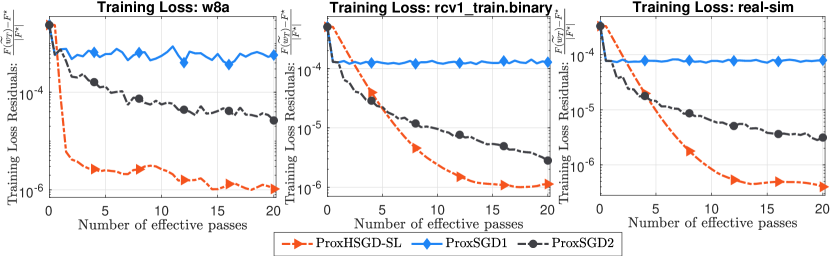
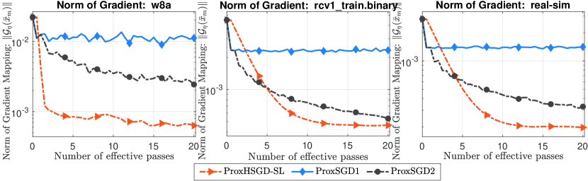
As we can observe from Figure 1 that our ProxHSGD-SL variant works relatively well and outperforms both ProxSGD1 and ProxSGD2. However, it then slows down or is saturated at a certain value of the loss function, probably due to the effect of the SGD term $u_{t}$ in our estimator $v_{t}$. It is not surprise that ProxSGD2 works better than ProxSGD1 due to the use of a scheduled diminishing learning rate.

$\mathrm{(b)}$ Single-loop methods with mini-batch:

Next, we test ProxHSGD-SL, ProxSGD1, and ProxSGD2 with mini-batches on six different datasets. We use the mini-batch size $\hat{b}:=50$ for w8a, rcv1-binary, real-sim, and news20.binary, $\hat{b}:=300$ for epsilon, and $\hat{b}:=500$ for url_combined. For ProxSpiderBoost and ProxSVRG, we set the mini-batch sizes as stated in Subsection 6.1.

For three small datasets, as suggested by Theorem 5.1, after some simple experiments, we find that $c_{0}:=9$ and $c_{1}:=10$ for w8a, $c_{0}:=18$ and $c_{1}:=9$ for rcv1_train.binary, and $c_{0}:=30$ and $c_{1}:=15$ for real-sim work well. While we choose the same mini-batch size in ProxSGD1, and ProxSGD2 as described above, we again tune their learning rates to have the best performance. The results are shown in Figure 2.

Figure 2: The relative training loss residuals and the absolute gradient mapping norms of (46) on three small datasets: Single-loop with mini-batch.

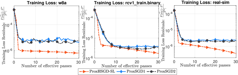
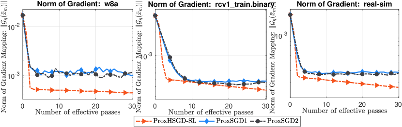
In this case, both ProxSGD1 and ProxSGD2 perform much better than the single sample case, and are comparable with ProxHSGD-SL. However, ProxHSGD-SL still outperforms ProxSGD1 and ProxSGD2 in the first and the last datasets, while it is slightly better than ProxSGD1 and ProxSGD2 in the second one.

Finally, we again evaluate three single-loop algorithms with mini-batches on three larger datasets: url_combined, epsilon, and news20.binary. Here, based on Theorem 5.1, we find that $c_{0}:=40\times 10^{3}$ and $c_{1}:=20$ for url_combined, $c_{0}:=15\times 10^{3}$ and $c_{1}:=30$ for epsilon, and $c_{0}:=10\times 10^{3}$ and $c_{1}:=20$ for news20.binary work well for our method. Figure 3 shows the convergence behavior of three algorithms.

Figure 3: The relative training loss residuals and the absolute gradient mapping norms of (46) on three large datasets: Single-loop with mini-batch.

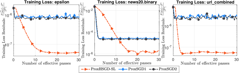
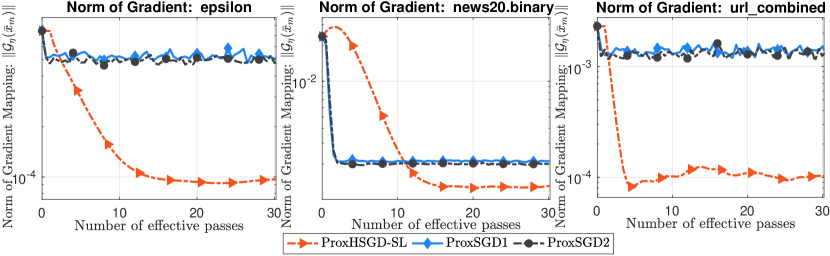
We obverse that from Figure 3 ProxHSGD-SL performs much better than ProxSGD1 and ProxSGD2, especially in the first and the third datasets. From the experiments (a) and (b), we believe that ProxHSGD-SL generally outperforms ProxSGD in these tests.

$\mathrm{(c)}$ Double-loop methods with mini-batch:

Our next test is on double-loop methods. We compare two different double-loop methods: ProxSVRG and ProxSpiderBoost with two restarting variants of Algorithm 2: ProxHSGD-RS1 and ProxHSGD-RS2. We use mini-batch for this test since ProxSpiderBoost only has guarantee for mini-batch variants.

First, let us test there algorithms using recommended learning rates and mini-batch sizes that have convergence guarantee. Note that both ProxSpiderBoost and ProxSVRG use a large learning rate $\eta:=\frac{1}{2L}$ and $\eta:=\frac{1}{3L}$, respectively. As observed in Pham2019 , these learning rates work well. We use our step-sizes and mini-batch sizes as suggested in Remark 6. To have a fair assessment, we also add a tuning variant (Tuned) of both ProxSpiderBoost and ProxSVRG, where we heuristically tune their learning rate to get the best performance. The results of this test are reported in Figure 4.

Figure 4: The relative training loss residuals and the absolute gradient mapping norms of (46) on three small datasets using both recommended (theoretical) and tuned step-sizes: Double-loop with mini-batch.

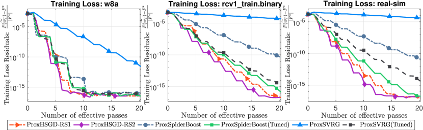
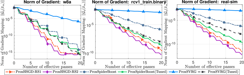
As we can see from Figure 4 that both ProxHSGD-RS1 and ProxHSGD-RS2 highly outperform ProxSVRG and ProxSpiderBoost, especially in the last two datasets. Due to the use of adaptive step-size, ProxHSGD-RS2 appears to be better than ProxHSGD-RS1. For the tuned learning rates, both ProxSVRG(Tuned) and ProxSpiderBoost(Tuned) are relatively comparable with ProxHSGD-RS1 and ProxHSGD-RS2 on these datasets. More precisely, ProxHSGD-RS1 and ProxHSGD-RS2 are slightly better than both ProxSVRG(Tuned) and ProxSpiderBoost(Tuned), especially in the last dataset. But, ProxSpiderBoost(Tuned) is still slightly better than ProxSVRG(Tuned) in the second and third datasets.

Now, we test these variants on three larger datasets: url_combined, epsilon, and news20.binary. Their performance is shown in Figure 5.

Figure 5: The relative training loss residuals and the absolute gradient mapping norms of (46) on three large datasets: Double-loop with mini-batch.

Without tuning learning rates, we observe similar behavior as in Figure 5, where our methods, ProxHSGD-RS1 and ProxHSGD-RS2, highly outperform ProxSVRG and are comparable with ProxSpiderBoost. Again, with tuned learning rates, ProxSVRG(Tuned) and ProxSpiderBoost(Tuned) are more comparable with ProxHSGD-RS1 and ProxHSGD-RS2, but our methods are still slightly better than their competitors in the second dataset. However, we do not observe significant difference between the the adaptive step-size variant, ProxHSGD-RS2 and the constant one, ProxHSGD-RS1, in this test.

6.3 Binary classification with nonconvex models

In this example, we consider the following binary classification model involving a nonconvex objective function and a convex regularizer broadly studied in the literature:

$${\min_{x\in\mathbb{R}^{p}}\left\{F(x):=\frac{1}{n}\sum_{i=1}^{n}\ell(a_{i}^{\top}x,b_{i})+\psi(x)\right\},\vspace{-0.5ex}}\vspace{-0.25ex}$$ (47)

where $\left\{(a_{i},b_{i})\right\}_{i=1}^{n}\subset\mathbb{R}^{p}\times\left\{-1,1\right\}^{n}$ is a given training dataset, $\psi$ is a convex regularizer, and $\ell(\cdot,\cdot)$ is a given smooth and nonconvex loss function. By setting $f_{i}(w):=\ell(a_{i}^{\top}w,b_{i})$ and choosing a convex regularizer $\psi$, we obtain the form (2) that satisfies Assumptions 1 and 2.

We consider the following settings for the choice of $\ell$ and $\psi$, where the first three models were studied in zhao2010convex , and the last one has been used in metel2019simple :

• Normalized sigmoid loss: $\ell_{1}(s,\tau):=1-\tanh(\tau s)$ for a given $\omega>0$ and $\psi(x):=\lambda\|x\|_{1}$. Here, $\ell_{1}(\cdot,\tau)$ is $L$-smooth with respect to $s$, where $L:\approx 0.7698$.

• Nonconvex loss in 2-layer neural networks: $\ell_{2}(s,\tau):=\left(1-\frac{1}{1+\exp(-\tau s)}\right)^{2}$ and $\psi(x):=\lambda\|x\|_{1}$. This function is also $L$-smooth with $L=0.15405$.

• Logistic difference loss: $\ell_{3}(s,\tau):=\ln(1+\exp(-\tau s))-\ln(1+\exp(-\tau s-1))$ and $\psi(x):=\lambda\|x\|_{1}$. This function is $L$-smooth with $L=0.092372$.

• Lorenz loss: $\ell_{4}(s,\tau):=\ln(1+(\tau s-1)^{2})$ if $\tau s\leq 1$, and $\ell_{4}(s,\tau)=0$, otherwise, and $\psi(x)=\lambda\|x\|_{1}$. This function is $L$-smooth with $L=4$.

We set the regularization parameter $\lambda:=\frac{1}{n}$ in all the tests which gives us relatively sparse solutions. We test the above algorithms on different scenarios ranging from small to large datasets using different algorithms.

$(a)$ Single-loop schemes with single-sample:

Our first experiment for (47) is on single-loop variants with single sample. For this test, we only choose the losses $\ell_{3}$ and $\ell_{4}$ with two well-known datasets: rcv1-binary and real-sim to avoid overloading the paper. The result of our test on the $\ell_{3}$-loss is shown in Figures 6 for three algorithms using the same setting as in Subsection 6.2, where we attempt to tune the learning rates for three competitors: ProxSGD1, ProxSGD2, and ProxSVRG.

Figure 6: The relative training loss residuals and the absolute gradient mapping norms of (47) with the nonconvex training loss $\ell_{3}$ on the two datasets: Single-loop with single-sample.

For the loss $\ell_{3}$ with $20$ epochs, ProxSGD1 and ProxSGD2 show their less competitive performance than our methods and ProxSVRG. While ProxSGD2 is not better than ProxSGD1 as observed in the previous example, ProxSVRG with tuned learning rate works really well and beats our ProxHSGD-SL. The restarting variants of our methods highly outperform ProxSGD1 and ProxSGD2 and is slightly better than ProxSVRG.

Additionally, the results of these six algorithms on the $\ell_{4}$-loss using the same setting are shown in Figure 7.

Figure 7: The relative training loss residuals and the absolute gradient mapping norms of (47) with the nonconvex training loss $\ell_{4}$ on the two datasets: Single-loop with single-sample.

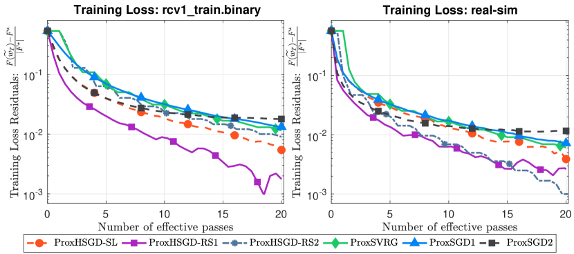
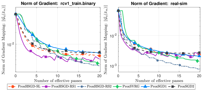
Figure 7 shows improved performance of both ProxSGD1, and ProxSGD2. In this case, these methods are comparable with our ProxHSGD-SL and ProxSVRG. However, our restarting variants, ProxHSGD-RS1 and ProxHSGD-RS2 are still slightly better than their competitors.

$\mathrm{(b)}$ Complete test on the mini-batch case:

Finally, we carry out a more thorough test on four different losses using two small datasets and two large datasets. We compare five different methods as shown in Tables 2 and 3. We report the relative training loss residuals, the absolute norms of gradient mapping, the training accuracy, and the test accuracy. Since ProxSVRG with the theoretical learning rate $1/3L$ performs quite poorly, we carry out a grid search between $[1/(15L),5/(3L)]$ to find a good learning rate for this experiment.

Table 2 reports the results on the two small datasets: rcv1_train.binary and real-sim after $20$ and $40$ epochs, respectively.

The loss function $\ell_{1}$
	Training Loss Residual		$\|G_{\eta}(w_{T})\|$		Training Accuracy		Test Accuracy
	​​20th ep.​​	​​40th ep.​​	​​20th ep.​​	​​40th ep.​​	​​20th ep.​​	​​40th ep.​​	​​20th ep.​​	​​40th ep.​​
Algorithms	rcv1_train.binary ($\boldsymbol{n=20,242,p=47,236}$)
ProxHSGD-SL​​	​​8.964e-02​​	​​3.409e-02​​	​​9.806e-05​​	​​3.043e-05​​	​​0.949​​	​​0.954​​	​​0.938​​	​​0.947​​
ProxHSGD-RS1​​	​​3.478e-02​​	​​1.888e-04​​	​​3.541e-05​​	​​1.586e-05​​	​​0.955​​	​​0.960​​	​​0.947​​	​​0.956​​
ProxSpiderBoost​​	​​1.649e-01​​	​​8.281e-02​​	​​2.664e-04​​	​​8.734e-05​​	​​0.944​​	​​0.950​​	​​0.934​​	​​0.938​​
ProxSVRG​​	​​2.918e-01​​	​​1.574e-01​​	​​1.578e-02​​	​​1.212e-02​​	​​0.626​​	​​0.825​​	​​0.004​​	​​0.561​​
ProxSGD2​​	​​1.505e-01​​	​​7.110e-02​​	​​2.446e-04​​	​​8.607e-05​​	​​0.945​​	​​0.951​​	​​0.936​​	​​0.941​​
Algorithms	real-sim ($\boldsymbol{n=72,309,p=20,958}$)
ProxHSGD-SL​​	​​4.554e-02​​	​​1.742e-02​​	​​1.377e-05​​	​​4.317e-06​​	​​0.977​​	​​0.981​​	​​0.659​​	​​0.647​​
ProxHSGD-RS1​​	​​1.756e-02​​	​​1.006e-04​​	​​4.699e-06​​	​​1.837e-06​​	​​0.981​​	​​0.984​​	​​0.646​​	​​0.634​​
ProxSpiderBoost​​	​​1.459e-01​​	​​8.004e-02​​	​​1.124e-04​​	​​3.537e-05​​	​​0.966​​	​​0.973​​	​​0.695​​	​​0.670​​
ProxSVRG​​	​​4.150e-02​​	​​2.443e-02​​	​​3.377e-03​​	​​1.783e-03​​	​​0.962​​	​​0.964​​	​​0.963​​	​​0.964​​
ProxSGD2​​	​​7.619e-02​​	​​3.613e-02​​	​​3.333e-05​​	​​1.087e-05​​	​​0.974​​	​​0.978​​	​​0.669​​	​​0.653​​
The loss function $\ell_{2}$
	Training Loss Residual		$\|G_{\eta}(w_{T})\|$		Training Accuracy		Test Accuracy
	​​20th ep.​​	​​40th ep.​​	​​20th ep.​​	​​40th ep.​​	​​20th ep.​​	​​40th ep.​​	​​20th ep.​​	​​40th ep.​​
Algorithms	rcv1_train.binary ($\boldsymbol{n=20,242,p=47,236}$)
ProxHSGD-SL​​	​​9.319e-03​​	​​1.229e-04​​	​​1.701e-03​​	​​9.506e-04​​	​​0.944​​	​​0.949​​	​​0.937​​	​​0.943​​
ProxHSGD-RS1​​	​​1.294e-02​​	​​2.546e-03​​	​​1.999e-03​​	​​1.107e-03​​	​​0.944​​	​​0.948​​	​​0.936​​	​​0.941​​
ProxSpiderBoost​​	​​2.593e-02​​	​​1.072e-02​​	​​3.146e-03​​	​​1.793e-03​​	​​0.940​​	​​0.944​​	​​0.931​​	​​0.936​​
ProxSVRG​​	​​2.927e-02​​	​​1.232e-02​​	​​3.445e-03​​	​​1.934e-03​​	​​0.939​​	​​0.944​​	​​0.929​​	​​0.934​​
ProxSGD2​​	​​4.545e-02​​	​​2.508e-02​​	​​6.103e-03​​	​​4.481e-03​​	​​0.935​​	​​0.940​​	​​0.926​​	​​0.930​​
Algorithms	real-sim ($\boldsymbol{n=72,309,p=20,958}$)
ProxHSGD-SL​​	​​8.850e-03​​	​​1.103e-04​​	​​1.339e-03​​	​​7.503e-04​​	​​0.968​​	​​0.971​​	​​0.665​​	​​0.650​​
ProxHSGD-RS1​​	​​1.294e-02​​	​​2.787e-03​​	​​1.626e-03​​	​​9.099e-04​​	​​0.966​​	​​0.970​​	​​0.673​​	​​0.655​​
ProxSpiderBoost​​	​​2.003e-02​​	​​6.730e-03​​	​​2.156e-03​​	​​1.179e-03​​	​​0.963​​	​​0.969​​	​​0.686​​	​​0.662​​
ProxSVRG​​	​​2.644e-02​​	​​1.150e-02​​	​​2.654e-03​​	​​1.521e-03​​	​​0.960​​	​​0.967​​	​​0.697​​	​​0.670​​
ProxSGD2​​	​​4.401e-02​​	​​2.249e-02​​	​​4.208e-03​​	​​2.562e-03​​	​​0.949​​	​​0.962​​	​​0.726​​	​​0.690​​
The loss function $\ell_{3}$
	Training Loss Residual		$\|G_{\eta}(w_{T})\|$		Training Accuracy		Test Accuracy
	​​20th ep.​​	​​40th ep.​​	​​20th ep.​​	​​40th ep.​​	​​20th ep.​​	​​40th ep.​​	​​20th ep.​​	​​40th ep.​​
Algorithms	rcv1_train.binary ($\boldsymbol{n=20,242,p=47,236}$)
ProxHSGD-SL​​	​​5.112e-02​​	​​1.915e-02​​	​​4.465e-03​​	​​2.663e-03​​	​​0.934​​	​​0.940​​	​​0.924​​	​​0.929​​
ProxHSGD-RS1​​	​​2.224e-02​​	​​6.492e-06​​	​​2.842e-03​​	​​1.626e-03​​	​​0.939​​	​​0.943​​	​​0.929​​	​​0.936​​
ProxSpiderBoost​​	​​2.850e-02​​	​​4.161e-03​​	​​3.188e-03​​	​​1.842e-03​​	​​0.938​​	​​0.943​​	​​0.928​​	​​0.935​​
ProxSVRG​​	​​2.797e-02​​	​​2.943e-03​​	​​3.157e-03​​	​​1.775e-03​​	​​0.938​​	​​0.943​​	​​0.928​​	​​0.935​​
ProxSGD2​​	​​1.316e-01​​	​​9.255e-02​​	​​9.639e-03​​	​​7.599e-03​​	​​0.924​​	​​0.929​​	​​0.919​​	​​0.922​​
Algorithms	real-sim ($\boldsymbol{n=72,309,p=20,958}$)
ProxHSGD-SL​​	​​2.873e-02​​	​​1.020e-02​​	​​1.859e-03​​	​​1.040e-03​​	​​0.962​​	​​0.968​​	​​0.687​​	​​0.662​​
ProxHSGD-RS1​​	​​1.196e-02​​	​​9.608e-07​​	​​1.114e-03​​	​​6.256e-04​​	​​0.968​​	​​0.970​​	​​0.663​​	​​0.647​​
ProxSpiderBoost​​	​​3.606e-02​​	​​1.442e-02​​	​​2.208e-03​​	​​1.218e-03​​	​​0.960​​	​​0.967​​	​​0.692​​	​​0.666​​
ProxSVRG​​	​​4.091e-02​​	​​1.862e-02​​	​​2.438e-03​​	​​1.403e-03​​	​​0.958​​	​​0.966​​	​​0.698​​	​​0.672​​
ProxSGD2​​	​​1.003e-01​​	​​5.911e-02​​	​​5.591e-03​​	​​3.493e-03​​	​​0.930​​	​​0.952​​	​​0.763​​	​​0.719​​
The loss function $\ell_{4}$
	Training Loss Residual		$\|G_{\eta}(w_{T})\|$		Training Accuracy		Test Accuracy
	​​20th ep.​​	​​40th ep.​​	​​20th ep.​​	​​40th ep.​​	​​20th ep.​​	​​40th ep.​​	​​20th ep.​​	​​40th ep.​​
Algorithms	rcv1_train.binary ($\boldsymbol{n=20,242,p=47,236}$)
ProxHSGD-SL​​	​​1.401e-02​​	​​1.819e-04​​	​​4.727e-03​​	​​2.674e-03​​	​​0.959​​	​​0.964​​	​​0.954​​	​​0.958​​
ProxHSGD-RS1​​	​​2.044e-02​​	​​4.125e-03​​	​​5.745e-03​​	​​3.253e-03​​	​​0.956​​	​​0.962​​	​​0.951​​	​​0.957​​
ProxSpiderBoost​​	​​2.422e-01​​	​​1.322e-01​​	​​4.045e-02​​	​​2.489e-02​​	​​0.926​​	​​0.935​​	​​0.920​​	​​0.927​​
ProxSVRG​​	​​2.635e-01​​	​​1.448e-01​​	​​4.304e-02​​	​​2.679e-02​​	​​0.925​​	​​0.933​​	​​0.920​​	​​0.926​​
ProxSGD2​​	​​3.686e-02​​	​​1.163e-02​​	​​9.593e-03​​	​​6.269e-03​​	​​0.952​​	​​0.959​​	​​0.943​​	​​0.953​​
Algorithms	real-sim ($\boldsymbol{n=72,309,p=20,958}$)
ProxHSGD-SL​​	​​9.009e-03​​	​​1.070e-04​​	​​2.386e-03​​	​​1.279e-03​​	​​0.981​​	​​0.984​​	​​0.683​​	​​0.676​​
ProxHSGD-RS1​​	​​1.106e-02​​	​​1.936e-03​​	​​2.450e-03​​	​​1.444e-03​​	​​0.981​​	​​0.984​​	​​0.679​​	​​0.674​​
ProxSpiderBoost​​	​​1.526e-01​​	​​8.450e-02​​	​​2.428e-02​​	​​1.168e-02​​	​​0.930​​	​​0.960​​	​​0.767​​	​​0.707​​
ProxSVRG​​	​​1.883e-01​​	​​1.076e-01​​	​​3.079e-02​​	​​1.558e-02​​	​​0.915​​	​​0.950​​	​​0.797​​	​​0.726​​
ProxSGD2​​	​​1.889e-02​​	​​6.334e-03​​	​​3.569e-03​​	​​2.267e-03​​	​​0.979​​	​​0.982​​	​​0.676​​	​​0.678​​

Table 2: The performance of $5$ different algorithms on two small datasets: The mini-batch case.

As can be seen from Table 2, either ProxHSGD-SL or ProxHSGD-RS1 is the best in these two datasets since they produce lower objective value and smaller gradient mapping norm. Three competitors ProxSpiderBoost, ProxSVRG, and ProxSGD2 are comparable with our methods in many cases, but in some other cases, our methods highly outperform these schemes. While our methods may produce better objective value and gradient mapping norm, we can observe that due to some overfitting issues, their test accuracy is slower than those of ProxSGD2 or ProxSVRG. This can be recognized by comparing the training accuracy and the corresponding test accuracy.

In addition, we run these five algorithms on the two larger datasets: news20.binary and url_combined. The results are reported in Table 3.

The loss function $\ell_{1}$
	Training Loss Residual		$\|G_{\eta}(w_{T})\|$		Training Accuracy		Test Accuracy
	​​20th ep.​​	​​40th ep.​​	​​20th ep.​​	​​40th ep.​​	​​20th ep.​​	​​40th ep.​​	​​20th ep.​​	​​40th ep.​​
Algorithms	news20.binary ($\boldsymbol{n=19,996,p=1,355,191}$)
ProxHSGD-SL​​	​​6.614e-02​​	​​1.990e-05​​	​​7.203e-03​​	​​4.471e-03​​	​​0.865​​	​​0.892​​	​​0.687​​	​​0.698​​
ProxHSGD-RS1​​	​​9.289e-02​​	​​1.764e-02​​	​​8.470e-03​​	​​5.173e-03​​	​​0.850​​	​​0.881​​	​​0.659​​	​​0.705​​
ProxSpiderBoost​​	​​2.932e-01​​	​​1.653e-01​​	​​1.558e-02​​	​​1.259e-02​​	​​0.626​​	​​0.822​​	​​0.003​​	​​0.544​​
ProxSVRG​​	​​3.073e-01​​	​​1.816e-01​​	​​1.301e-02​​	​​1.356e-02​​	​​0.625​​	​​0.812​​	​​0.001​​	​​0.500​​
ProxSGD2​​	​​2.733e-01​​	​​1.426e-01​​	​​2.212e-02​​	​​1.847e-02​​	​​0.649​​	​​0.832​​	​​0.015​​	​​0.585​​
Algorithms	url_combined ($\boldsymbol{n=2,396,130,p=3,231,961}$)
ProxHSGD-SL​​	​​5.934e-03​​	​​9.244e-05​​	​​6.157e-04​​	​​3.985e-04​​	​​0.968​​	​​0.970​​	​​0.969​​	​​0.971​​
ProxHSGD-RS1​​	​​7.405e-03​​	​​1.279e-03​​	​​6.615e-04​​	​​4.257e-04​​	​​0.968​​	​​0.970​​	​​0.968​​	​​0.970​​
ProxSpiderBoost​​	​​2.467e-02​​	​​1.396e-02​​	​​1.789e-03​​	​​1.015e-03​​	​​0.964​​	​​0.966​​	​​0.964​​	​​0.966​​
ProxSVRG​​	​​4.581e-02​​	​​2.690e-02​​	​​3.824e-03​​	​​1.992e-03​​	​​0.962​​	​​0.964​​	​​0.963​​	​​0.964​​
ProxSGD2​​	​​2.013e-02​​	​​1.101e-02​​	​​1.478e-03​​	​​8.988e-04​​	​​0.965​​	​​0.967​​	​​0.965​​	​​0.967​​
The loss function $\ell_{2}$
	Training Loss Residual		$\|G_{\eta}(w_{T})\|$		Training Accuracy		Test Accuracy
	​​20th ep.​​	​​40th ep.​​	​​20th ep.​​	​​40th ep.​​	​​20th ep.​​	​​40th ep.​​	​​20th ep.​​	​​40th ep.​​
Algorithms	news20.binary ($\boldsymbol{n=19,996,p=1,355,191}$)
ProxHSGD-SL​​	​​3.636e-02​​	​​2.190e-02​​	​​2.977e-03​​	​​2.006e-03​​	​​0.791​​	​​0.826​​	​​0.451​​	​​0.604​​
ProxHSGD-RS1​​	​​1.055e-02​​	​​1.831e-06​​	​​1.367e-03​​	​​8.706e-04​​	​​0.844​​	​​0.864​​	​​0.638​​	​​0.633​​
ProxSpiderBoost​​	​​3.476e-02​​	​​2.042e-02​​	​​2.849e-03​​	​​1.899e-03​​	​​0.797​​	​​0.829​​	​​0.481​​	​​0.615​​
ProxSVRG​​	​​3.726e-02​​	​​2.203e-02​​	​​3.025e-03​​	​​1.997e-03​​	​​0.788​​	​​0.826​​	​​0.445​​	​​0.606​​
ProxSGD2​​	​​6.471e-02​​	​​5.196e-02​​	​​7.270e-03​​	​​6.595e-03​​	​​0.625​​	​​0.691​​	​​0.003​​	​​0.112​​
Algorithms	url_combined ($\boldsymbol{n=2,396,130,p=3,231,961}$)
ProxHSGD-SL​​	​​6.055e-03​​	​​3.834e-03​​	​​3.613e-04​​	​​2.308e-04​​	​​0.966​​	​​0.969​​	​​0.966​​	​​0.969​​
ProxHSGD-RS1​​	​​2.241e-03​​	​​3.597e-08​​	​​1.584e-04​​	​​1.220e-04​​	​​0.971​​	​​0.973​​	​​0.971​​	​​0.973​​
ProxSpiderBoost​​	​​6.305e-03​​	​​3.949e-03​​	​​3.643e-04​​	​​2.210e-04​​	​​0.966​​	​​0.969​​	​​0.966​​	​​0.969​​
ProxSVRG​​	​​1.058e-02​​	​​6.839e-03​​	​​7.481e-04​​	​​4.049e-04​​	​​0.964​​	​​0.965​​	​​0.964​​	​​0.966​​
ProxSGD2​​	​​1.449e-02​​	​​9.151e-03​​	​​1.173e-03​​	​​6.126e-04​​	​​0.962​​	​​0.964​​	​​0.963​​	​​0.964​​
The loss function $\ell_{3}$
	Training Loss Residual		$\|G_{\eta}(w_{T})\|$		Training Accuracy		Test Accuracy
	​​20th ep.​​	​​40th ep.​​	​​20th ep.​​	​​40th ep.​​	​​20th ep.​​	​​40th ep.​​	​​20th ep.​​	​​40th ep.​​
Algorithms	news20.binary ($\boldsymbol{n=19,996,p=1,355,191}$)
ProxHSGD-SL​​	​​4.182e-02​​	​​1.890e-02​​	​​3.482e-03​​	​​2.518e-03​​	​​0.691​​	​​0.787​​	​​0.115​​	​​0.451​​
ProxHSGD-RS1​​	​​2.163e-02​​	​​7.406e-06​​	​​2.636e-03​​	​​1.737e-03​​	​​0.782​​	​​0.819​​	​​0.435​​	​​0.586​​
ProxSpiderBoost​​	​​2.663e-02​​	​​4.377e-03​​	​​2.846e-03​​	​​1.902e-03​​	​​0.765​​	​​0.814​​	​​0.365​​	​​0.564​​
ProxSVRG​​	​​3.048e-02​​	​​6.860e-03​​	​​3.012e-03​​	​​2.002e-03​​	​​0.750​​	​​0.810​​	​​0.314​​	​​0.549​​
ProxSGD2​​	​​7.544e-02​​	​​6.249e-02​​	​​6.868e-03​​	​​6.169e-03​​	​​0.623​​	​​0.625​​	​​0.001​​	​​0.003​​
Algorithms	url_combined ($\boldsymbol{n=2,396,130,p=3,231,961}$)
ProxHSGD-SL​​	​​1.048e-02​​	​​5.507e-03​​	​​5.294e-04​​	​​2.958e-04​​	​​0.964​​	​​0.966​​	​​0.965​​	​​0.966​​
ProxHSGD-RS1​​	​​2.601e-03​​	​​3.495e-08​​	​​1.926e-04​​	​​1.193e-04​​	​​0.968​​	​​0.970​​	​​0.969​​	​​0.970​​
ProxSpiderBoost​​	​​7.921e-03​​	​​3.722e-03​​	​​4.022e-04​​	​​2.293e-04​​	​​0.965​​	​​0.967​​	​​0.965​​	​​0.968​​
ProxSVRG​​	​​1.615e-02​​	​​8.911e-03​​	​​8.411e-04​​	​​4.496e-04​​	​​0.963​​	​​0.965​​	​​0.964​​	​​0.965​​
ProxSGD2​​	​​3.364e-02​​	​​1.886e-02​​	​​1.945e-03​​	​​1.005e-03​​	​​0.962​​	​​0.963​​	​​0.962​​	​​0.964​​
The loss function $\ell_{4}$
	Training Loss Residual		$\|G_{\eta}(w_{T})\|$		Training Accuracy		Test Accuracy
	​​20th ep.​​	​​40th ep.​​	​​20th ep.​​	​​40th ep.​​	​​20th ep.​​	​​40th ep.​​	​​20th ep.​​	​​40th ep.​​
Algorithms	news20.binary ($\boldsymbol{n=19,996,p=1,355,191}$)
ProxHSGD-SL​​	​​4.252e-02​​	​​6.483e-04​​	​​7.475e-03​​	​​4.661e-03​​	​​0.883​​	​​0.914​​	​​0.694​​	​​0.669​​
ProxHSGD-RS1​​	​​6.343e-02​​	​​1.603e-02​​	​​9.342e-03​​	​​5.527e-03​​	​​0.865​​	​​0.901​​	​​0.676​​	​​0.675​​
ProxSpiderBoost​​	​​2.381e-01​​	​​2.017e-01​​	​​1.962e-02​​	​​1.812e-02​​	​​0.624​​	​​0.627​​	​​0.001​​	​​0.004​​
ProxSVRG​​	​​2.426e-01​​	​​2.072e-01​​	​​2.005e-02​​	​​1.828e-02​​	​​0.624​​	​​0.626​​	​​0.001​​	​​0.003​​
ProxSGD2​​	​​1.007e-01​​	​​3.930e-02​​	​​2.068e-02​​	​​1.704e-02​​	​​0.843​​	​​0.884​​	​​0.573​​	​​0.688​​
Algorithms	url_combined ($\boldsymbol{n=2,396,130,p=3,231,961}$)
ProxHSGD-SL​​	​​4.997e-03​​	​​7.821e-05​​	​​8.616e-04​​	​​4.849e-04​​	​​0.953​​	​​0.956​​	​​0.951​​	​​0.955​​
ProxHSGD-RS1​​	​​5.779e-03​​	​​1.309e-03​​	​​8.034e-04​​	​​5.427e-04​​	​​0.951​​	​​0.954​​	​​0.950​​	​​0.953​​
ProxSpiderBoost​​	​​2.159e-02​​	​​1.574e-02​​	​​3.250e-03​​	​​1.895e-03​​	​​0.949​​	​​0.947​​	​​0.948​​	​​0.946​​
ProxSVRG​​	​​4.104e-02​​	​​2.319e-02​​	​​9.529e-03​​	​​3.680e-03​​	​​0.954​​	​​0.949​​	​​0.953​​	​​0.948​​
ProxSGD2​​	​​8.181e-03​​	​​3.501e-03​​	​​1.555e-03​​	​​7.355e-04​​	​​0.950​​	​​0.952​​	​​0.949​​	​​0.951​​

Table 3: The performance of $5$ different algorithms on two large datasets: The mini-batch case.

Again, we observe the same performance among these methods. Either ProxHSGD-SL or ProxHSGD-RS1 works best for every case. Three other competiors: ProxSGD, ProxSVRG, and ProxSpiderBoost work well and are relatively comparable with our methods in some cases, but they are still slower than our methods overall.

6.4 Feedforward neural network training problem

In the last example, we consider the following composite nonconvex optimization problem obtained from a fully connected feedforward neural network training task:

$${\min_{x\in\mathbb{R}^{p}}\left\{F(x):=\frac{1}{n}\sum_{i=1}^{n}\ell\big{(}F_{L}(x,a_{i}),b_{i}\big{)}+\psi(x)\right\},}\vspace{-0.25ex}$$ (48)

where we concatenate all the weight matrices and bias vectors of the neural network in one vector of variable $x$, $\left\{(a_{i},b_{i})\right\}_{i=1}^{n}$ is a training dataset, $F_{L}(\cdot)$ is a composition between all linear transforms and activation functions as $F_{L}(x,a):=\boldsymbol{\sigma}_{L}(W_{L}\boldsymbol{\sigma}_{L-1}(W_{L-1}\boldsymbol{\sigma}_{L-2}(\cdots\boldsymbol{\sigma}_{0}(W_{0}a+\mu_{0})\cdots)+\mu_{L-1})+\mu_{L})$, where $W_{i}$ is a weight matrix, $\mu_{i}$ is a bias vector, $\boldsymbol{\sigma}_{i}$ is an activation function, $L$ is the number of layers, $\ell(\cdot)$ is a cross-entropy loss, and $\psi(x):=\lambda\|x\|_{1}$ is the $\ell_{1}$-norm regularizer for some $\lambda>0$ to obtain sparse weights. By defining $f_{i}(x):=\ell(F_{L}(x,a_{i}),b_{i})$ for $i=1,\cdots,n$, we can formulate (48) into the composite finite-sum setting (2).

We implement mini-batch variants of Algorithm 1 and Algorithm 2, and compare with two other methods: ProxSVRG and ProxSpiderBoost in TensorFlow using the well-known dataset mnist to evaluate their performance.

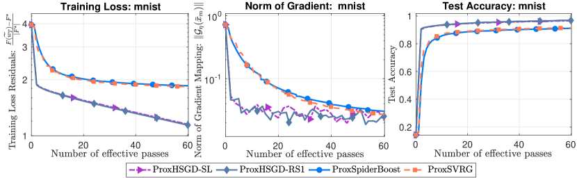
In the first experiment, we use an one-hidden-layer-fully-connected neural network: $784\times 128\times 10$, while in the second test, we increase the number of neurons in the hidden layer to obtain another fully-connected neural network: $784\times 800\times 10$. The activation function $\boldsymbol{\sigma}_{i}$ for the hidden layer is ReLU, and for the output layer is soft-max.

Our experiment configuration is as follows. We choose $\lambda:=\frac{1}{n}$ to obtain sparse weights. We set $\gamma=0.95$ for all methods and tune $\eta$ to obtain the best results. Here, we obtain $\eta=0.3$ for ProxHSGD-SL and ProxHSGD-RS1. We also tune $\eta$ in ProxSpiderBoost and ProxSVRG to obtain the best results. We finally get $\eta=0.12$ for ProxSpiderBoost and $\eta=0.2$ for ProxSVRG. We set $\hat{b}:=100$ for our algorithms, $\hat{b}:=\lfloor\sqrt{n}\rfloor$ for ProxSpiderBoost, and $\hat{b}:=\lfloor n^{2/3}\rfloor$ for ProxSVRG and set the epoch length $m:=\lfloor\frac{n}{\hat{b}}\rfloor$. The performance of the four algorithms running on the first network is reported in Figure 8.

Figure 8: The performance (training loss, norm of gradient mapping, and test accuracy) of $4$ algorithms on the mnist dataset for solving (48): A fully-connected $784\times 128\times 10$ neural network.

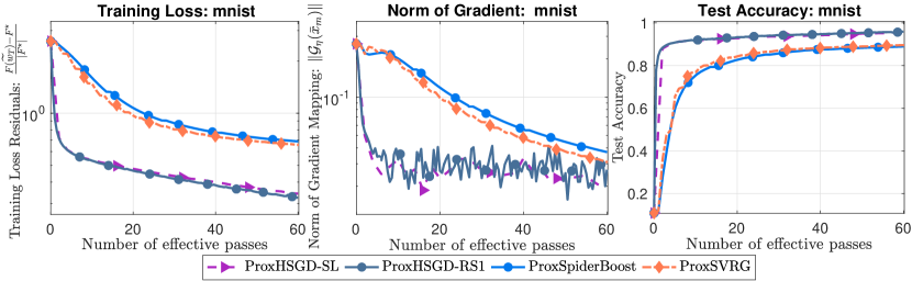
From Figure 8, both ProxHSGD-SL and ProxHSGD-RS1 work relatively well in this example, and outperform two other methods. On one hand, our methods achieve better training loss values, norms of gradient mapping, and test accuracy than both ProxSpiderBoost and ProxSVRG. On the other hand, the restarting variant ProxHSGD-RS1 appears to be slightly better than ProxHSGD-SL.

Figure 9: The performance (training loss, norm of gradient mapping, and test accuracy) of $4$ algorithms on the mnist dataset for solving (48): A fully-connected $784\times 800\times 10$ neural network.

Besides, the results when running these algorithms on the second neural network are given in Figure 9. We can observe the same behavior of these four algorithms as in Figure 8, but ProxHSGD-RS1 does not exhibit clear advantage over ProxHSGD-SL.

Appendix A Appendix: Properties of Hybrid Stochastic Estimators

This appendix provides the full proof of our theoretical results in Section 3. However, we also need the following lemma in the sequel. Hence, we prove it here.

Lemma 7

Given $L>0$, $\delta>0$, $\epsilon>0$, and $\omega\in(0,1)$, let $\{\gamma_{t}\}_{t=0}^{m}$ be the sequence updated by

$${\gamma_{m}:=\frac{\delta}{L}~{}~{}~{}~{}\text{and}~{}~{}~{}~{}\gamma_{t}:=\frac{\delta}{L+\epsilon L^{2}\big{[}\omega\gamma_{t+1}+\omega^{2}\gamma_{t+2}+\cdots+\omega^{(m-t)}\gamma_{m}\big{]}},}\vspace{-0.25ex}$$ (49)

for $t=0,\cdots,m-1$. Then

$${0<\gamma_{0}<\gamma_{1}<\cdots<\gamma_{m}=\frac{\delta}{L}~{}~{}~{}\text{and}~{}~{}~{}\Sigma_{m}:=\sum_{t=0}^{m}\gamma_{t}\geq\frac{\delta(m+1)\sqrt{1-\omega}}{L\left[\sqrt{1-\omega}+\sqrt{1-\omega+4\delta\omega\epsilon}\right]}.}\vspace{-0.25ex}$$ (50)

Proof

First, from (49) it is obvious to show that $0<\gamma_{0}<\cdots<\gamma_{m-1}=\frac{\delta}{L(1+\epsilon\omega)}<\gamma_{m}=\frac{\delta}{L}$. At the same time, since $\omega\in(0,1)$, we have $1\geq\omega\geq\omega^{2}\geq\cdots\geq\omega^{m}$. By Chebyshev’s sum inequality, we have

$${\begin{array}[]{ll}(m-t)\big{(}\omega\gamma_{t+1}+\omega^{2}\gamma_{t+2}+\cdots+\omega^{m-t}\gamma_{m}\big{)}&\leq\big{(}\sum_{j=t+1}^{m}\gamma_{i}\big{)}\left(\omega+\omega^{2}+\cdots+\omega^{m-t}\right)\vspace{1ex}\\ &\leq\frac{\omega}{1-\omega}\big{(}\sum_{j=t+1}^{m}\gamma_{i}\big{)}.\end{array}}\vspace{-0.25ex}$$ (51)

From the update (49), we also have

$${\left\{\begin{array}[]{ll}\epsilon L^{2}\gamma_{0}(\omega\gamma_{1}+\omega^{2}\gamma_{2}+\cdots+\omega^{m}\gamma_{m})&=\delta-L\gamma_{0}\vspace{1ex}\\ \epsilon L^{2}\gamma_{1}(\omega\gamma_{2}+\omega^{2}\gamma_{3}+\cdots+\omega^{m-1}\gamma_{m})&=\delta-L\gamma_{1}\vspace{1ex}\\ \cdots&\cdots\vspace{1ex}\\ \epsilon L^{2}\gamma_{m-1}\omega\gamma_{m}&=\delta-L\gamma_{m-1}\vspace{1ex}\\ 0&=\delta-L\gamma_{m}.\end{array}\right.}\vspace{-0.25ex}$$ (52)

Substituting (51) into (52), we get

$${\left\{\begin{array}[]{ll}\frac{\omega\epsilon L^{2}}{1-\omega}\gamma_{0}(\gamma_{0}+\gamma_{1}+\cdots+\gamma_{m})&\geq\delta m-mL\gamma_{0}+\frac{\omega\epsilon L^{2}}{1-\omega}\gamma_{0}^{2}\vspace{1ex}\\ \frac{\omega\epsilon L^{2}}{1-\omega}\gamma_{1}(\gamma_{0}+\gamma_{1}+\cdots+\gamma_{m})&\geq\delta(m-1)-(m-1)L\gamma_{1}+\frac{\omega\epsilon L^{2}}{1-\omega}(\gamma_{1}\gamma_{0}+\gamma_{1}^{2})\vspace{1ex}\\ \cdots&\cdots\vspace{1ex}\\ \frac{\omega\epsilon L^{2}}{1-\omega}\gamma_{m-1}(\gamma_{0}+\gamma_{1}+\cdots+\gamma_{m})&\geq\delta-L\gamma_{m-1}+\frac{\omega\epsilon L^{2}}{1-\omega}(\gamma_{m-1}\gamma_{0}+\cdots+\gamma_{m-1}^{2})\vspace{1ex}\\ \frac{\omega\epsilon L^{2}}{1-\omega}\gamma_{m}(\gamma_{0}+\gamma_{1}+\cdots+\gamma_{m})&\geq\delta-L\gamma_{m}+\frac{\omega\epsilon L^{2}}{1-\omega}(\gamma_{m}\gamma_{0}+\cdots+\gamma_{m}^{2}).\end{array}\right.}\vspace{-0.25ex}$$

Let us define $\Sigma_{m}:=\sum_{t=0}^{m}\gamma_{t}$ and $S_{m}:=\sum_{t=0}^{m}\gamma_{t}^{2}$. Summing up both sides of the above inequalities, we get

$${\frac{\omega\epsilon L^{2}}{1-\omega}\Sigma_{m}^{2}\geq\frac{\delta(m^{2}+m+2)}{2}-L(m\gamma_{0}+(m-1)\gamma_{1}+\cdots+\gamma_{m-1}+\gamma_{m})+\frac{\omega\epsilon L^{2}}{2(1-\omega)}\big{(}S_{m}+\Sigma_{m}^{2}\big{)}.}\vspace{-0.25ex}$$

Using again Chebyshev’s sum inequality, we have

$${m\gamma_{0}+(m-1)\gamma_{1}+\cdots+\gamma_{m-1}+\gamma_{m}\leq\frac{m^{2}+m+2}{2(m+1)}\left(\sum_{t=0}^{m}\gamma_{t}\right)=\frac{(m^{2}+m+2)\Sigma_{m}}{2(m+1)}.}\vspace{-0.25ex}$$

Note that $(m+1)S_{m}\geq\Sigma_{m}^{2}$ by Cauchy-Schwarz’s inequality, which shows that $S_{m}+\Sigma_{m}^{2}\geq\big{(}\frac{m+2}{m+1}\big{)}\Sigma_{m}^{2}$. Combining three last inequalities, we obtain the following quadratic inequation in $\Sigma_{m}>0$:

$${\frac{m\omega\epsilon L^{2}}{(1-\omega)}\Sigma_{m}^{2}+L(m^{2}+m+2)\Sigma_{m}-\delta(m+1)(m^{2}+m+2)\geq 0.}\vspace{-0.25ex}$$

Solving this inequation with respect to $\Sigma_{m}>0$, we obtain

$${\begin{array}[]{ll}\Sigma_{m}&\geq\frac{(1-\omega)\big{[}\sqrt{(m^{2}+m+2)^{2}+\frac{4m(m+1)(m^{2}+m+2)\omega\epsilon\delta}{1-\omega}}-(m^{2}+m+2)\big{]}}{2\epsilon\omega mL}\vspace{1ex}\\ &=\frac{2\delta(m+1)}{L\left[1+\sqrt{1+\frac{4m(m+1)\omega\delta\epsilon}{(1-\omega)(m^{2}+m+2)}}\right]}\vspace{1ex}\\ &\geq\frac{2\delta(m+1)\sqrt{1-\omega}}{L\left[\sqrt{1-\omega}+\sqrt{1-\omega+4\delta\omega\epsilon}\right]}~{}~{}~{}~{}~{}\text{since}~{}~{}\frac{m(m+1)}{m^{2}+m+2}<1.\end{array}}\vspace{-0.25ex}$$

This proves (50).

A.1 The proof of Lemma 3: Variance estimate with mini-batch

The proof of the first expression of (19) is the same as in Lemma 1. We only prove the second one. Let $\Delta_{\mathcal{B}_{t}}:=\frac{1}{b_{t}}\sum_{i\in\mathcal{B}_{t}}\left[G_{\xi_{i}}(x_{t})-G_{\xi_{i}}(x_{t-1})\right]$, $\Delta_{t}:=G(x_{t})-G(x_{t-1})$, $\hat{\delta}_{t}:=\hat{v}_{t}-G(x_{t})$, and $\delta{u}_{t}:=u_{t}-G(x_{t})$. Clearly, we have

$${\mathbb{E}_{\mathcal{B}_{t}}\left[\Delta_{\mathcal{B}_{t}}\right]=\Delta_{t}~{}~{}~{}\text{and}~{}~{}~{}\mathbb{E}_{\hat{\mathcal{B}}_{t}}\left[\delta{u}_{t}\right]=0.}\vspace{-0.25ex}$$

Moreover, we can rewrite $\hat{v}_{t}$ as

$${\hat{\delta}_{t}=\beta_{t-1}\hat{\delta}_{t-1}+\beta_{t-1}\Delta_{\mathcal{B}_{t}}+(1-\beta_{t-1})\delta{u}_{t}-\beta_{t-1}\Delta_{t}.}\vspace{-0.25ex}$$

Therefore, using these two expressions, we can derive

$${\begin{array}[]{lcl}\mathbb{E}_{(\mathcal{B}_{t},\hat{\mathcal{B}}_{t})}\left[\|\hat{\delta}_{t}\|^{2}\right]&=&\beta_{t-1}^{2}\|\hat{\delta}_{t-1}\|^{2}+\beta_{t-1}^{2}\mathbb{E}_{\mathcal{B}_{t}}\left[\|\Delta_{\mathcal{B}_{t}}\|^{2}\right]+(1-\beta_{t-1})^{2}\mathbb{E}_{\hat{\mathcal{B}}_{t}}\left[\|\delta{u}_{t}\|^{2}\right]+\beta_{t-1}^{2}\|\Delta_{t}\|^{2}\vspace{1ex}\\ &&+{~{}}2\beta_{t-1}^{2}\langle\hat{\delta}_{t-1},\mathbb{E}_{\mathcal{B}_{t}}\left[\Delta_{\mathcal{B}_{t}}\right]\rangle+2\beta_{t-1}(1-\beta_{t-1})\langle\hat{\delta}_{t-1},\mathbb{E}_{\hat{\mathcal{B}}_{t}}\left[\delta{u}_{t}\right]\rangle-2\beta_{t-1}^{2}\langle\hat{\delta}_{t-1},\Delta_{t}\rangle\vspace{1ex}\\ &&+{~{}}2\beta_{t-1}(1-\beta_{t-1})\mathbb{E}_{(\mathcal{B}_{t},\hat{\mathcal{B}}_{t})}\left[\langle\Delta_{\mathcal{B}_{t}},\delta{u}_{t}\rangle\right]-2\beta_{t-1}^{2}\langle\mathbb{E}_{\mathcal{B}_{t}}\left[\Delta_{\mathcal{B}_{t}}\right],\Delta_{t}\rangle\vspace{1ex}\\ &&-{~{}}2\beta_{t-1}(1-\beta_{t-1})\langle\mathbb{E}_{\hat{\mathcal{B}}_{t}}\left[\delta{u}_{t}\right],\Delta_{t}\rangle\vspace{1ex}\\ &=&\beta_{t-1}^{2}\|\hat{\delta}_{t-1}\|^{2}+\beta_{t-1}^{2}\mathbb{E}_{\mathcal{B}_{t}}\left[\|\Delta_{\mathcal{B}_{t}}\|^{2}\right]+(1-\beta_{t-1})^{2}\mathbb{E}_{\hat{\mathcal{B}}_{t}}\left[\|\delta{u}_{t}\|^{2}\right]-\beta_{t-1}^{2}\|\Delta_{t}\|^{2}.\end{array}}\vspace{-0.25ex}$$

Similar to the proof of (Pham2019, , Lemma 2), for the finite-sum case (i.e., $|\Omega|=n$), we can show that

$${\mathbb{E}_{\mathcal{B}_{t}}\left[\|\Delta_{\mathcal{B}_{t}}\|^{2}\right]=\frac{n(b_{t}-1)}{(n-1)b_{t}}\|\Delta_{t}\|^{2}+\frac{(n-b_{t})}{(n-1)b_{t}}\mathbb{E}_{\xi}\left[\|G_{\xi}(x_{t})-G_{\xi}(x_{t-1})\|^{2}\right].}\vspace{-0.25ex}$$

For the expectation case, we have

$${\mathbb{E}_{\mathcal{B}_{t}}\left[\|\Delta_{\mathcal{B}_{t}}\|^{2}\right]=\left(1-\frac{1}{b_{t}}\right)\|\Delta_{t}\|^{2}+\frac{1}{b_{t}}\mathbb{E}_{\xi}\left[\|G_{\xi}(x_{t})-G_{\xi}(x_{t-1})\|^{2}\right].}\vspace{-0.25ex}$$

Using the definition of $\rho$ in Lemma 4, we can unify these two expressions as

$${\mathbb{E}_{\mathcal{B}_{t}}\left[\|\Delta_{\mathcal{B}_{t}}\|^{2}\right]=\left(1-\rho\right)\|\Delta_{t}\|^{2}+\rho\mathbb{E}_{\xi}\left[\|G_{\xi}(x_{t})-G_{\xi}(x_{t-1})\|^{2}\right].}\vspace{-0.25ex}$$

Substituting the last expression into the previous one, we obtain the second expression of (19). $\square$

A.2 The proof of Lemma 4: Upper bound of mini-batch variance

From Lemma 3, taking the expectation with respect to $\mathcal{F}_{t+1}:=\sigma(x_{0},\mathcal{B}_{0},\hat{\mathcal{B}}_{0},\cdots,\mathcal{B}_{t},\hat{\mathcal{B}}_{t})$, we have

$${\begin{array}[]{lcl}\mathbb{E}\left[\|\hat{v}_{t}-G(x_{t})\|^{2}\right]&\leq&\beta_{t-1}^{2}\mathbb{E}\left[\|\hat{v}_{t-1}-G(x_{t-1})\|^{2}\right]\vspace{1ex}\\ &&+{~{}}\rho L^{2}\beta_{t-1}^{2}\mathbb{E}\left[\|x_{t}-x_{t-1}\|^{2}\right]+(1-\beta_{t-1})^{2}\mathbb{E}_{\hat{\mathcal{B}}_{t}}\left[\|u_{t}-G(x_{t})\|^{2}\right].\end{array}}\vspace{-0.25ex}$$

In addition, from (Pham2019, , Lemma 2), we have $\mathbb{E}_{\hat{\mathcal{B}}_{t}}\left[\|u_{t}-G(x_{t})\|^{2}\right]\leq\hat{\rho}\mathbb{E}_{\xi}\left[\|G_{\xi}(x_{t})-G(x_{t})\|^{2}\right]=\hat{\rho}\sigma_{t}^{2}$, where $\sigma_{t}^{2}:=\mathbb{E}_{\xi}\left[\|G_{\xi}(x_{t})-G(x_{t})\|^{2}\right]$.

Let $A_{t}^{2}:=\mathbb{E}\left[\|\hat{v}_{t}-G(x_{t})\|^{2}\right]$ and $B_{t}^{2}:=\mathbb{E}\left[\|x_{t+1}-x_{t}\|^{2}\right]$. Then, the above estimate can be upper bounded as follows:

$${A_{t}^{2}\leq\beta_{t-1}^{2}A_{t-1}^{2}+\rho L^{2}\beta_{t-1}^{2}B_{t-1}^{2}+\hat{\rho}(1-\beta_{t-1})^{2}\sigma_{t}^{2}.}\vspace{-0.25ex}$$

By following inductive step as in the proof of Lemma 2, we obtain from the last inequality that

$${\begin{array}[]{lcl}A_{t}^{2}&\leq&\left(\beta_{t-1}^{2}\cdots\beta_{0}^{2}\right)A_{0}^{2}+\rho L^{2}\left(\beta_{t-1}^{2}\cdots\beta_{0}^{2}\right)B_{0}^{2}+\cdots+\rho L^{2}\beta_{t-1}^{2}B_{t-1}^{2}\vspace{1ex}\\ &&+{~{}}\hat{\rho}\left[\left(\beta_{t-1}^{2}\cdots\beta_{1}^{2}\right)(1-\beta_{0})^{2}\sigma_{1}^{2}+\cdots+(1-\beta_{t-1})^{2}\sigma_{t}^{2}\right].\end{array}}\vspace{-0.25ex}$$

Using the definition of $\omega_{t}$, $\omega_{i,t}$, and $S_{t}$ from (16), the previous inequality becomes

$${A_{t}^{2}\leq\omega_{t}A_{0}^{2}+\rho L^{2}\sum_{i=0}^{t-1}\omega_{i,t}B_{i}^{2}+\hat{\rho}S_{t},}\vspace{-0.25ex}$$

which is the same as (20) by substituting the definition of $A_{t}$ and $B_{t}$ above into it. $\square$

Appendix B The Proof of Technical Results in Section 4: The Single Sample Case

We provide the full proof of technical results in Section 4.

B.1 The proof of Lemma 2: Key estimate

From the update $x_{t+1}:=(1-\gamma_{t})x_{t}+\gamma_{t}\widehat{x}_{t+1}$ at Step 8 of Algorithm 1, we have $x_{t+1}-x_{t}=\gamma_{t}(\widehat{x}_{t+1}-x_{t})$. From the $L$-average smoothness condition in Assumption 2, one can write

$${\begin{array}[]{ll}f(x_{t+1})&\leq f(x_{t})+\langle\nabla f(x_{t}),x_{t+1}-x_{t}\rangle+\frac{L}{2}\|x_{t+1}-x_{t}\|^{2}\\ &=f(x_{t})+\gamma_{t}\langle\nabla f(x_{t}),\widehat{x}_{t+1}-x_{t}\rangle+\frac{L\gamma_{t}^{2}}{2}\|\widehat{x}_{t+1}-x_{t}\|^{2}.\end{array}}\vspace{-0.25ex}$$ (53)

Using convexity of $\psi$, we can show that

$${\psi(x_{t+1})\leq(1-\gamma_{t})\psi(x_{t})+\gamma_{t}\psi(\widehat{x}_{t+1})\leq\psi(x_{t})+\gamma_{t}\langle\nabla\psi(\widehat{x}_{t+1}),\widehat{x}_{t+1}-x_{t}\rangle,}\vspace{-0.25ex}$$ (54)

where $\nabla\psi(\widehat{x}_{t+1})\in\partial\psi(\widehat{x}_{t+1})$ is any subgradient of $\psi$ at $\widehat{x}_{t+1}$.

Utilizing the optimality condition of $\widehat{x}_{t+1}=\mathrm{prox}_{\eta_{t}\psi}(x_{t}-\eta_{t}v_{t})$, we can show that $\nabla\psi(\widehat{x}_{t+1})=-v_{t}-\frac{1}{\eta_{t}}(\widehat{x}_{t+1}-x_{t})$ for some $\nabla\psi(\widehat{x}_{t+1})\in\partial\psi(\widehat{x}_{t+1})$. Substituting this relation into (54), we get

$${\psi(x_{t+1})\leq\psi(x_{t})-\gamma_{t}\left\langle v_{t},\widehat{x}_{t+1}-x_{t}\right\rangle-\frac{\gamma_{t}}{\eta_{t}}\|\widehat{x}_{t+1}-x_{t}\|^{2}.}\vspace{-0.25ex}$$ (55)

Combining (53) and (55), and using $F(x):=f(x)+\psi(x)$ from (1), we obtain

$${F(x_{t+1})\leq F(x_{t})+\gamma_{t}\left\langle\nabla f(x_{t})-v_{t},\widehat{x}_{t+1}-x_{t}\right\rangle-\left(\frac{\gamma_{t}}{\eta_{t}}-\frac{L\gamma_{t}^{2}}{2}\right)\|\widehat{x}_{t+1}-x_{t}\|^{2}.}\vspace{-0.25ex}$$ (56)

For any $c_{t}>0$, we can always write

$${\begin{array}[]{ll}\langle\nabla f(x_{t})-v_{t},\widehat{x}_{t+1}-x_{t}\rangle&=\frac{1}{2c_{t}}\|\nabla f(x_{t})-v_{t}\|^{2}+\frac{c_{t}}{2}\|\widehat{x}_{t+1}-x_{t}\|^{2}\vspace{1ex}\\ &-\frac{1}{2c_{t}}\|\nabla f(x_{t})-v_{t}-c_{t}(\widehat{x}_{t+1}-x_{t})\|^{2}.\end{array}}\vspace{-0.25ex}$$

Utilizing this expression, we can rewrite as

$${F(x_{t+1})\leq F(x_{t})+\frac{\gamma_{t}}{2c_{t}}\|\nabla{f}(x_{t}-v_{t}\|^{2}-\left(\frac{\gamma_{t}}{\eta_{t}}-\frac{L\gamma_{t}^{2}}{2}-\frac{\gamma_{t}c_{t}}{2}\right)\|\widehat{x}_{t+1}-x_{t}\|^{2}-\frac{\tilde{\sigma}_{t}^{2}}{2}.}\vspace{-0.25ex}$$

where $\tilde{\sigma}_{t}^{2}:=\frac{\gamma_{t}}{c_{t}}\|\nabla{f}(x_{t}-v_{t}-c_{t}(\widehat{x}_{t+1}-x_{t})\|^{2}\geq 0$.

Taking expectation both sides of this inequality over the entire history $\mathcal{F}_{t+1}$, we obtain

$${\begin{array}[]{ll}\mathbb{E}\left[F(x_{t+1})\right]&\leq\mathbb{E}\left[F(x_{t})\right]+\frac{\gamma_{t}}{2c_{t}}\mathbb{E}\left[\|\nabla{f}(x_{t})-v_{t}\|^{2}\right]\vspace{1ex}\\ &-{~{}}\Big{(}\frac{\gamma_{t}}{\eta_{t}}-\frac{L\gamma_{t}^{2}}{2}-\frac{\gamma_{t}c_{t}}{2}\Big{)}\mathbb{E}\left[\|\widehat{x}_{t+1}-x_{t}\|^{2}\right]-\frac{1}{2}\mathbb{E}\left[\tilde{\sigma}_{t}^{2}\right].\end{array}}\vspace{-0.25ex}$$ (57)

Next, from the definition of gradient mapping $\mathcal{G}_{\eta}(x):=\frac{1}{\eta}\left(x-\mathrm{prox}_{\eta\psi}(x-\eta\nabla f(x))\right)$ in (9), we can see that

$${\eta_{t}\|\mathcal{G}_{\eta_{t}}(x_{t})\|=\|x_{t}-\mathrm{prox}_{\eta_{t}\psi}\left(x_{t}-\eta_{t}\nabla f(x_{t})\right)\|.}\vspace{-0.25ex}$$

Using this expression, the triangle inequality, and the nonexpansive property $\|\mathrm{prox}_{\eta\psi}(z)-\mathrm{prox}_{\eta\psi}(w)\|\leq\|z-w\|$ of $\mathrm{prox}_{\eta\psi}$, we can derive that

$${\begin{array}[]{ll}\eta_{t}\|\mathcal{G}_{\eta_{t}}(x_{t})\|&\leq\|\widehat{x}_{t+1}-x_{t}\|+\|\mathrm{prox}_{\eta_{t}\psi}(x_{t}-\eta_{t}\nabla{f}(x_{t}))-\widehat{x}_{t+1}\|\vspace{1ex}\\ &=\|\widehat{x}_{t+1}-x_{t}\|+\|\mathrm{prox}_{\eta_{t}\psi}(x_{t}-\eta_{t}\nabla{f}(x_{t}))-\mathrm{prox}_{\eta_{t}\psi}(x_{t}-\eta_{t}v_{t})\|\vspace{1ex}\\ &\leq\|\widehat{x}_{t+1}-x_{t}\|+\eta_{t}\|\nabla{f}(x_{t})-v_{t}\|.\end{array}}\vspace{-0.25ex}$$

Now, for any $r_{t}>0$, the last estimate leads to

$${\eta_{t}^{2}\mathbb{E}\left[\|\mathcal{G}_{\eta_{t}}(x_{t})\|^{2}\right]\leq\left(1+\tfrac{1}{r_{t}}\right)\mathbb{E}\left[\|\widehat{x}_{t+1}-x_{t}\|^{2}\right]+(1+r_{t})\eta_{t}^{2}\mathbb{E}\left[\|\nabla{f}(x_{t})-v_{t}\|^{2}\right].}\vspace{-0.25ex}$$

Multiplying this inequality by $\frac{q_{t}}{2}>0$ and adding the result to (57), we finally get

$${\begin{array}[]{ll}\mathbb{E}\left[F(x_{t+1})\right]&\leq\mathbb{E}\left[F(x_{t})\right]-\frac{q_{t}\eta_{t}^{2}}{2}\mathbb{E}\left[\|\mathcal{G}_{\eta_{t}}(x_{t})\|^{2}\right]\vspace{1ex}\\ &+{~{}}\frac{1}{2}\Big{[}\frac{\gamma_{t}}{c_{t}}+(1+r_{t})q_{t}\eta_{t}^{2}\Big{]}\mathbb{E}\left[\|\nabla{f}(x_{t})-v_{t}\|^{2}\right]\vspace{1ex}\\ &-{~{}}\frac{1}{2}\Big{[}\frac{2\gamma_{t}}{\eta_{t}}-L\gamma_{t}^{2}-\gamma_{t}c_{t}-q_{t}\left(1+\frac{1}{r_{t}}\right)\Big{]}\mathbb{E}\left[\|\widehat{x}_{t+1}-x_{t}\|^{2}\right]-\frac{1}{2}\mathbb{E}\left[\tilde{\sigma}_{t}^{2}\right].\end{array}}\vspace{-0.25ex}$$

Using the definition of $\theta_{t}$ and $\kappa_{t}$ from (22), i.e.,:

$${\theta_{t}:=\frac{\gamma_{t}}{c_{t}}+(1+r_{t})q_{t}\eta_{t}^{2}~{}~{}~{}~{}\text{and}~{}~{}~{}~{}\kappa_{t}:=\frac{2\gamma_{t}}{\eta_{t}}-L\gamma_{t}^{2}-\gamma_{t}c_{t}-q_{t}\left(1+\frac{1}{r_{t}}\right),}\vspace{-0.25ex}$$

we can simplify this estimate as follows:

$${\begin{array}[]{ll}\mathbb{E}\left[F(x_{t+1})\right]&\leq\mathbb{E}\left[F(x_{t})\right]-\frac{q_{t}\eta_{t}^{2}}{2}\mathbb{E}\left[\|\mathcal{G}_{\eta_{t}}(x_{t})\|^{2}\right]+\frac{\theta_{t}}{2}\mathbb{E}\left[\|\nabla{f}(x_{t})-v_{t}\|^{2}\right]\vspace{1ex}\\ &-{~{}}\frac{\kappa_{t}}{2}\mathbb{E}\left[\|\widehat{x}_{t+1}-x_{t}\|^{2}\right]-\frac{1}{2}\mathbb{E}\left[\tilde{\sigma}_{t}^{2}\right].\end{array}}\vspace{-0.25ex}$$ (58)

This is exactly (21). $\square$

B.2 The proof of Lemma 6: Key estimate of Lyapunov function

From (14), by taking the full expectation on the history $\mathcal{F}_{t+1}$ and using the $L$-average smoothness of $f$, we can show that

$${{\!\!\!\!\!\!\!}\begin{array}[]{ll}\mathbb{E}\left[\|v_{t+1}-\nabla{f}(x_{t+1})\|^{2}\right]{\!\!\!}&\leq\beta_{t}^{2}\mathbb{E}\left[\|v_{t}-\nabla{f}(x_{t})\|^{2}\right]+\beta_{t}^{2}L^{2}\mathbb{E}\left[\|x_{t+1}-x_{t}\|^{2}\right]+(1-\beta_{t})^{2}\sigma_{t+1}^{2}\vspace{1ex}\\ &=\beta_{t}^{2}\mathbb{E}\left[\|v_{t}-\nabla{f}(x_{t})\|^{2}\right]+\beta_{t}^{2}\gamma_{t}^{2}L^{2}\mathbb{E}\left[\|\widehat{x}_{t+1}-x_{t}\|^{2}\right]+(1-\beta_{t})^{2}\sigma_{t+1}^{2},\end{array}{\!\!\!\!\!\!\!}}\vspace{-0.25ex}$$

where $\sigma_{t}^{2}:=\mathbb{E}\left[\|\nabla{f}_{\zeta_{t}}(x_{t})-\nabla{f}(x_{t})\|^{2}\right]$.

Let $V$ be the Lyapunov function defined by (23). Then, by multiplying the last inequality by $\frac{\alpha_{t+1}}{2}>0$, adding the result to (58), and then using this Lyapunov function we can show that

$${\begin{array}[]{ll}V(x_{t+1})&\leq V(x_{t})-\frac{q_{t}\eta_{t}^{2}}{2}\mathbb{E}\left[\|\mathcal{G}_{\eta_{t}}(x_{t})\|^{2}\right]-\frac{1}{2}(\alpha_{t}-\beta_{t}^{2}\alpha_{t+1}-\theta_{t})\mathbb{E}\left[\|v_{t}-\nabla{f}(x_{t})\|^{2}\right]\vspace{1.25ex}\\ &-{~{}}\frac{1}{2}(\kappa_{t}-\alpha_{t+1}\beta_{t}^{2}\gamma_{t}^{2}L^{2})\mathbb{E}\left[\|\widehat{x}_{t+1}-x_{t}\|^{2}\right]+\frac{1}{2}(1-\beta_{t})^{2}\alpha_{t+1}\sigma_{t+1}^{2}-\frac{1}{2}\mathbb{E}\left[\tilde{\sigma}_{t}^{2}\right].\end{array}}\vspace{-0.25ex}$$ (59)

Let us choose $\gamma_{t}$, $\eta_{t}$, and other parameters such that the conditions (24) hold, i.e.:

$${\alpha_{t}-\beta_{t}^{2}\alpha_{t+1}-\theta_{t}\geq 0~{}~{}~{}\text{and}~{}~{}\kappa_{t}-\alpha_{t+1}\beta_{t}^{2}\gamma_{t}^{2}L^{2}\geq 0.}\vspace{-0.25ex}$$

In this case, (59) can be simplified as follows:

$${V(x_{t+1})\leq V(x_{t})-\frac{q_{t}\eta_{t}^{2}}{2}\mathbb{E}\left[\|\mathcal{G}_{\eta_{t}}(x_{t})\|^{2}\right]+\frac{1}{2}\alpha_{t+1}(1-\beta_{t})^{2}\sigma_{t+1}^{2}.}\vspace{-0.25ex}$$

This proves (25).

Finally, summing up this inequality from $t:=0$ to $t:=m$, we obtain

$${\sum_{t=0}^{m}\frac{q_{t}\eta_{t}^{2}}{2}\mathbb{E}\left[\|\mathcal{G}_{\eta_{t}}(x_{t})\|^{2}\right]\leq V(x_{0})-V(x_{m+1})+\frac{1}{2}\sum_{t=0}^{m}\alpha_{t+1}(1-\beta_{t})^{2}\sigma_{t+1}^{2}.}\vspace{-0.25ex}$$

Note that $V(x_{m+1}):=\mathbb{E}\left[F(x_{m+1})\right]+\frac{\alpha_{m+1}}{2}\mathbb{E}\left[\|v_{m+1}-\nabla{f}(x_{m+1})\|^{2}\right]\geq\mathbb{E}\left[F(x_{m+1})\right]\geq F^{\star}$ by Assumption 1 and $V(x_{0})=F(x_{0})+\frac{\alpha_{0}}{2}\mathbb{E}\left[\|v_{0}-\nabla{f}(x_{0})\|^{2}\right]$. Using these estimates into the last inequality, we obtain the key estimate (26). $\square$

B.3 The proof of Theorem 4.2: The adaptive step-size case

Let $\{(x_{t},\hat{x}_{t})\}$ be generated by Algorithm 1. Let us again choose $c_{t}:=L$, $r_{t}:=1$ and $q_{t}:=\frac{L\gamma_{t}}{2}$ and fix $\eta_{t}:=\eta\in(0,\frac{1}{L})$ in Lemma 2 as done in Theorem 4.1. Then, from (22), we have

$${\theta_{t}:=\frac{(1+L^{2}\eta^{2})\gamma_{t}}{L}~{}~{}~{}~{}~{}\text{and}~{}~{}~{}~{}~{}\kappa_{t}:=\left(\frac{2}{\eta}-L\gamma_{t}-2L\right)\gamma_{t}.}\vspace{-0.25ex}$$

Using these parameters into (21) and summing up the result from $t:=0$ to $t:=m$, and then using (15) from Lemma 2, we obtain

$${\begin{array}[]{lcl}\mathbb{E}\left[F(x_{m+1})\right]&\leq&\mathbb{E}\left[F(x_{0})\right]+\dfrac{L^{2}}{2}\displaystyle\sum_{t=0}^{m}\theta_{t}\sum_{i=0}^{t-1}\gamma_{i}^{2}\omega_{i,t}\mathbb{E}\left[\|\widehat{x}_{i+1}-x_{i}\|^{2}\right]\vspace{1ex}\\ &&-{~{}}\dfrac{1}{2}\displaystyle\sum_{t=0}^{m}\kappa_{t}\mathbb{E}\left[\|\widehat{x}_{t+1}-x_{t}\|^{2}\right]-\dfrac{\eta^{2}L}{4}\displaystyle\sum_{t=0}^{m}\gamma_{t}\mathbb{E}\left[\|\mathcal{G}_{\eta}(x_{t})\|^{2}\right]\vspace{1ex}\\ &&-{~{}}\displaystyle\sum_{t=0}^{m}\mathbb{E}\left[\tilde{\sigma}_{t}\right]+\dfrac{1}{2}\displaystyle\sum_{t=0}^{m}\theta_{t}\omega_{t}\bar{\sigma}^{2}+\dfrac{1}{2}\displaystyle\sum_{t=0}^{m}\theta_{t}S_{t},\end{array}}\vspace{-0.25ex}$$

where $\bar{\sigma}^{2}:=\mathbb{E}\left[\|v_{0}-\nabla f(x_{0})\|^{2}\right]\geq 0$, $\tilde{\sigma}_{t}^{2}:=\dfrac{\gamma_{t}}{2}\|\nabla f(x_{t})-v_{t}-L(\hat{x}_{t+1}-x_{t})\|^{2}\geq 0$, and $\omega_{i,t}$, $\omega_{t}$, and $S_{t}$ are defined in Lemma 2.

By ignoring the nonnegative term $\mathbb{E}\left[\tilde{\sigma}_{t}^{2}\right]$, and using the expression of $\theta_{t}$ and $\kappa_{t}$ above, we can further estimate the last inequality as follows:

$${\begin{array}[]{lcl}\mathbb{E}\left[F(x_{m+1})\right]&\leq&\mathbb{E}\left[F(x_{0})\right]-\frac{\eta^{2}L}{4}\displaystyle\sum_{t=0}^{m}\gamma_{t}\mathbb{E}\left[\|\mathcal{G}_{\eta}(x_{t})\|^{2}\right]\vspace{1ex}\\ &&+~{}\frac{(1+L^{2}\eta^{2})\bar{\sigma}^{2}}{2L}{\displaystyle\sum_{t=0}^{m}\omega_{t}\gamma_{t}}+\frac{(1+L^{2}\eta^{2})}{2L}{\displaystyle\sum_{t=0}^{m}\gamma_{t}S_{t}}+\frac{\mathcal{T}_{m}}{2},\end{array}}\vspace{-0.25ex}$$ (60)

where $\mathcal{T}_{m}$ is defined as follows:

$${{\!\!\!}\mathcal{T}_{m}:=L(1+L^{2}\eta^{2})\sum_{t=0}^{m}\gamma_{t}\sum_{i=0}^{t-1}\omega_{i,t}\gamma_{i}^{2}\mathbb{E}\left[\|\widehat{x}_{i+1}-x_{i}\|^{2}\right]-\sum_{t=0}^{m}\gamma_{t}\left(\frac{2}{\eta}-2L-L\gamma_{t}\right)\mathbb{E}\left[\|\widehat{x}_{i+1}-x_{i}\|^{2}\right].{\!\!\!}}\vspace{-0.25ex}$$ (61)

Now, with the choice of $\beta_{t}=\beta:=1-\frac{1}{\sqrt{\tilde{b}(m+1)}}\in(0,1)$, we can easily show that $\omega_{t}=\beta^{2t}$, $\omega_{i,t}=\beta^{2(t-i)}$, and $s_{t}:=\big{(}\prod_{j=i+2}^{t}\beta_{j-1}^{2}\big{)}(1-\beta_{i})^{2}=(1-\beta)^{2}\Big{[}\frac{1-\beta^{2t}}{1-\beta^{2}}\Big{]}<\frac{1-\beta}{1+\beta}$ due to Lemma 2.

Let $w_{i}^{2}:=\mathbb{E}\left[\|\widehat{x}_{i+1}-x_{i}\|^{2}\right]$. To bound the quantity $\mathcal{T}_{m}$ defined by (61), we note that

$${\begin{array}[]{lcl}\displaystyle\sum_{t=1}^{m}\gamma_{t}\sum_{i=0}^{t-1}\beta^{2(t-i)}\gamma_{i}^{2}w_{i}^{2}&=&\beta^{2}\gamma_{0}^{2}\big{[}\gamma_{1}+\beta^{2}\gamma_{2}+\cdots+\beta^{2(m-1)}\gamma_{m}\big{]}w_{0}^{2}\vspace{1ex}\\ &&+{~{}}\beta^{2}\gamma_{1}^{2}\big{[}\gamma_{2}+\beta^{2}\gamma_{3}+\cdots+\beta^{2(m-2)}\gamma_{m}\big{]}w_{1}^{2}+\cdots\vspace{1.5ex}\\ &&+{~{}}\beta^{2}\gamma_{m-2}^{2}\big{[}\gamma_{m-1}+\beta^{2}\gamma_{m}\big{]}w_{m-2}^{2}+\beta^{2}\gamma_{m-1}^{2}\gamma_{m}w_{m-1}^{2}.\end{array}}\vspace{-0.25ex}$$

Using $\delta:=\frac{2}{\eta}-2L$, we can write $\mathcal{T}_{m}$ from (61) as

$${\begin{array}[]{lcl}\mathcal{T}_{m}&=&\gamma_{0}\Big{[}L(1+L^{2}\eta^{2})\beta^{2}\gamma_{0}\big{[}\gamma_{1}+\beta^{2}\gamma_{2}+\cdots+\beta^{2(m-1)}\gamma_{m}\big{]}-(\delta-L\gamma_{0})\Big{]}w_{0}^{2}\vspace{1ex}\\ &&+{~{}}\gamma_{1}\Big{[}L(1+L^{2}\eta^{2})\beta^{2}\gamma_{1}\big{[}\gamma_{2}+\beta^{2}\gamma_{3}+\cdots+\beta^{2(m-2)}\gamma_{m}\big{]}-(\delta-L\gamma_{1})\Big{]}w_{1}^{2}+\cdots\vspace{1ex}\\ &&+{~{}}\gamma_{m-1}\Big{[}L(1+L^{2}\eta^{2})\beta^{2}\gamma_{m-1}\gamma_{m}-(1-L\gamma_{m-1})\Big{]}w_{m-1}^{2}-\gamma_{m}(\delta-L\gamma_{m})w_{m}^{2}.\end{array}}\vspace{-0.25ex}$$

To guarantee $\mathcal{T}_{m}\leq 0$, from the last expression of $\mathcal{T}_{m}$, we can impose the following condition:

$${\left\{\begin{array}[]{lcl}L(1+L^{2}\eta^{2})\beta^{2}\gamma_{0}\big{[}\gamma_{1}+\beta^{2}\gamma_{2}+\cdots+\beta^{2(m-1)}\gamma_{m}\big{]}-(\delta-L\eta_{0})&=&0\vspace{1ex}\\ L(1+L^{2}\eta^{2})\beta^{2}\gamma_{1}\big{[}\gamma_{2}+\beta^{2}\gamma_{3}+\cdots+\beta^{2(m-2)}\gamma_{m}\big{]}-(\delta-L\eta_{1})&=&0\vspace{1ex}\\ \cdots\cdots&\cdots&\vspace{1ex}\\ L(1+L^{2}\eta^{2})\beta^{2}\gamma_{m-1}\gamma_{m}-(\delta-L\gamma_{m-1})&=&0\vspace{1ex}\\ -(1-L\eta_{m})&=&0.\end{array}\right.}\vspace{-0.25ex}$$ (62)

It is obvious to show that the condition (62) leads to the following update of $\gamma_{t}$:

$${\gamma_{m}:=\frac{\delta}{L}~{}~{}~{}\text{and}~{}~{}~{}\gamma_{t}:=\frac{\delta}{L+L(1+L^{2}\eta^{2})\big{[}\beta^{2}\gamma_{t+1}+\beta^{4}\gamma_{t+2}+\cdots+\beta^{2(m-t)}\gamma_{m}\big{]}},~{}~{}~{}t=0,\cdots,m-1,}\vspace{-0.25ex}$$

which is exactly (33).

(a)  Since $\beta=1-\frac{1}{[\tilde{b}(m+1)]^{1/2}}$, we have

$${\frac{1}{[\tilde{b}(m+1)]^{1/2}}=1-\beta\leq 1-\beta^{2}\leq\frac{2}{[\tilde{b}(m+1)]^{1/2}}.}\vspace{-0.25ex}$$

Moreover, since $\eta\in(0,\frac{1}{L})$, with $\epsilon:=\frac{1+L^{2}\eta^{2}}{L}$, $\delta:=\frac{2}{\eta}-2L$, and $\omega:=\beta^{2}\in(0,1)$, using the last inequalities, we can easily show that

$${\sqrt{1-\omega}+\sqrt{1-\omega+4\delta\omega\epsilon}=\sqrt{1-\beta^{2}}+\sqrt{1-\beta^{2}+\frac{4\delta\beta^{2}(1+L^{2}\eta^{2})}{L}}\leq 2\sqrt{2}\left(\frac{1}{[\tilde{b}(m+1)]^{1/4}}+\sqrt{\frac{\delta}{L}}\right).}\vspace{-0.25ex}$$ (63)

Using (63), $\sqrt{1-\omega}=\sqrt{1-\beta^{2}}\geq\frac{1}{(\tilde{b}(m+1))^{1/4}}$, and $\epsilon=\frac{1+L^{2}\eta^{2}}{L}$ into (50) of Lemma 7, we can derive

$${\Sigma_{m}:=\sum_{t=0}^{m}\gamma_{t}\geq\frac{\delta(m+1)}{2\sqrt{2}\left(L+\sqrt{L\delta}[\tilde{b}(m+1)]^{1/4}\right)}.}\vspace{-0.25ex}$$ (64)

Next, since $\omega_{t}=\beta^{2t}$, by Chebyshev’s sum inequality, we have

$${\sum_{t=0}^{m}\omega_{t}\gamma_{t}=\sum_{t=0}^{m}\beta^{2t}\gamma_{t}\leq\frac{\Sigma_{m}}{(m+1)}(1+\beta^{2}+\cdots+\beta^{2m})\leq\frac{\Sigma_{m}}{(m+1)(1-\beta^{2})}.}\vspace{-0.25ex}$$

Utilizing this estimate, $\bar{\sigma}^{2}:=\mathbb{E}\left[\|v_{0}-\nabla{f}(x_{0})\|^{2}\right]\leq\frac{\sigma^{2}}{\tilde{b}}$, and $S_{t}\leq\sigma^{2}s_{t}\leq\frac{(1-\beta)\sigma^{2}}{1+\beta}$ into (60), and noting that $\mathcal{T}_{m}\leq 0$, we can further upper bound it as

$${\displaystyle\frac{\eta^{2}L}{4}\displaystyle\sum_{t=0}^{m}\gamma_{t}\mathbb{E}\left[\|\mathcal{G}_{\eta}(x_{t})\|^{2}\right]\leq F(x_{0})-\mathbb{E}\left[F(x_{m+1})\right]+\frac{(1+L^{2}\eta^{2})\sigma^{2}\Sigma_{m}}{2L(1-\beta^{2})(m+1)\tilde{b}}+\frac{(1+L^{2}\eta^{2})(1-\beta)\sigma^{2}\Sigma_{m}}{2L(1+\beta)}.}\vspace{-0.25ex}$$

By Assumption 1, we have $\mathbb{E}\left[F(x_{m+1})\right]\geq F^{\star}$. Substituting this bound into the last estimate and then multiplying the result by $\frac{4}{L\eta^{2}\Sigma_{m}}$ we obtain

$${\displaystyle\frac{1}{\Sigma_{m}}\displaystyle\sum_{t=0}^{m}\gamma_{t}\mathbb{E}\left[\|\mathcal{G}_{\eta}(x_{t})\|^{2}\right]\leq\frac{4}{L\eta^{2}\Sigma_{m}}[F(x_{0})-F^{\star}]+\frac{2\sigma^{2}(1+L^{2}\eta^{2})}{L^{2}\eta^{2}(1+\beta)}\left[\frac{1}{\tilde{b}(m+1)(1-\beta)}+(1-\beta)\right].}\vspace{-0.25ex}$$

Since $\beta=1-\frac{1}{\tilde{b}^{1/2}(m+1)^{1/2}}$, we have $\frac{1}{\tilde{b}(m+1)(1-\beta)}+(1-\beta)=\frac{2}{\tilde{b}^{1/2}(m+1)^{1/2}}$. Utilizing this expression, (64), $1+\eta^{2}L^{2}\leq 2$, and $\beta\in[0,1]$, we can further upper bound the last estimate as

$${\displaystyle\frac{1}{\Sigma_{m}}\displaystyle\sum_{t=0}^{m}\gamma_{t}\mathbb{E}\left[\|\mathcal{G}_{\eta}(x_{t})\|^{2}\right]\leq\frac{8\sqrt{2}\big{(}L+\sqrt{\delta L}[\tilde{b}(m+1)]^{1/4}\big{)}}{L\eta^{2}\delta(m+1)}\left[F(x_{0})-F^{\star}\right]+\frac{8\sigma^{2}}{L^{2}\eta^{2}[\tilde{b}(m+1)]^{1/2}}.}\vspace{-0.25ex}$$ (65)

In addition, due to the choice of $\overline{x}_{m}\sim\mathbb{U}_{\mathbf{p}}\left(\{x_{t}\}_{t=0}^{m}\right)$, we have $\mathbb{E}\left[\|\mathcal{G}_{\eta}(\overline{x}_{m})\|^{2}\right]=\displaystyle\frac{1}{\Sigma_{m}}\displaystyle\sum_{t=0}^{m}\gamma_{t}\mathbb{E}\left[\|\mathcal{G}_{\eta}(x_{t})\|^{2}\right]$. Combining this expression and (65), we obtain (34).

(b)  Let us choose $\tilde{b}:=c_{1}^{2}(m+1)^{1/3}$ for some constant $c_{1}>0$. Since $\beta=1-\frac{1}{[\tilde{b}(m+1)]^{1/2}}$, to guarantee $\beta\geq 0$, we need to impose $c_{1}\geq\frac{1}{(m+1)^{2/3}}$. With this choice of $\tilde{b}$, (34) reduces to

$${\mathbb{E}\left[\|\mathcal{G}_{\eta}(\overline{x}_{m})\|^{2}\right]\leq\frac{8}{L^{2}\eta^{2}(m+1)^{2/3}}\left[\frac{\sqrt{2}L\big{(}L+\sqrt{c_{1}L\delta}\big{)}}{\delta}\big{[}F(x_{0})-F^{\star}\big{]}+\frac{\sigma^{2}}{c_{1}}\right].}\vspace{-0.25ex}$$

Let us denote by $\Delta_{0}:=\frac{8}{L^{2}\eta^{2}}\left[\frac{\sqrt{2}L(L+\sqrt{c_{1}L\delta})}{\delta}\big{[}F(x_{0})-F^{\star}\big{]}+\frac{\sigma^{2}}{c_{1}}\right]$. Then, similar to the proof of Theorem 4.1, we can show that the number of iterations $m$ is at most $m:=\left\lfloor\frac{\Delta_{0}^{3/2}}{\varepsilon^{3}}\right\rfloor$, and the total number $\mathcal{T}_{m}$ of stochastic gradient evaluations $\nabla{f}_{\xi}(x_{t})$ is at most $\mathcal{T}_{m}:=\left\lfloor\frac{c_{1}^{2}\Delta_{0}^{1/2}}{\varepsilon}+\frac{3\Delta_{0}^{3/2}}{\varepsilon^{3}}\right\rfloor$. $\square$

B.4 The proof of Theorem 4.3: The restarting variant

(a)  Since we use the adaptive variant of Algorithm 1 as stated in Theorem 4.2 for the inner loop of Algorithm 2, from (65), we can see that at each stage $s$, the following estimate holds

$${\displaystyle\frac{1}{\Sigma_{m}}\displaystyle\sum_{t=0}^{m}\gamma_{t}\mathbb{E}\left[\|\mathcal{G}_{\eta}(x_{t}^{(s)})\|^{2}\right]\leq\frac{8\sqrt{2}\tilde{b}^{1/4}\left(L+\sqrt{L\delta}\right)}{L\eta^{2}\delta(m+1)^{3/4}}\mathbb{E}\left[F(x_{0}^{(s)})-F(x_{m+1}^{(s)})\right]+\frac{8\sigma^{2}}{L^{2}\eta^{2}[\tilde{b}(m+1)]^{1/2}}.}\vspace{-0.25ex}$$ (66)

where we use the superscript “^(s)” to indicate the stage $s$ in Algorithm 2. Summing up this inequality from $s:=1$ to $s:=S$, and then multiplying the result by $\frac{1}{S}$ and using $\mathbb{E}\left[F(x_{m+1}^{(S)})\right]\geq F^{\star}>-\infty$, and $\mathbb{E}\left[\|\mathcal{G}_{\eta}(\overline{x}_{T})\|^{2}\right]=\dfrac{1}{S\Sigma_{m}}\displaystyle\sum_{s=1}^{S}\sum_{t=0}^{m}\mathbb{E}\left[\|\mathcal{G}_{\eta}(x_{t}^{(s)})\|^{2}\right]$, we get (35), i.e.:

$${\begin{array}[]{lcl}\mathbb{E}\left[\|\mathcal{G}_{\eta}(\overline{x}_{T})\|^{2}\right]&=&\dfrac{1}{S\Sigma_{m}}\displaystyle\sum_{s=1}^{S}\sum_{t=0}^{m}\mathbb{E}\left[\|\mathcal{G}_{\eta}(x_{t}^{(s)})\|^{2}\right]\vspace{1ex}\\ &\leq&\dfrac{8\sqrt{2}\tilde{b}^{1/4}\big{(}L+\sqrt{L\delta}\big{)}}{L\delta\eta^{2}S(m+1)^{3/4}}\big{[}F(\overline{x}^{(0)})-F^{\star}\big{]}+\dfrac{8\sigma^{2}}{L^{2}\eta^{2}[\tilde{b}(m+1)]^{1/2}}.\end{array}}\vspace{-0.25ex}$$ (67)

(b) Let $\Delta_{F}:=F(\overline{x}^{(0)})-F^{\star}>0$ and choose $\tilde{b}:=c_{1}^{2}(m+1)$ for some constant $c_{1}>0$. Since $\beta=1-\frac{1}{[\tilde{b}(m+1)]^{1/2}}\in(0,1)$, we need to choose $c_{1}$ such that $c_{1}\geq\frac{1}{m+1}$.

Now, for any tolerance $\varepsilon>0$, to guarantee $\mathbb{E}\left[\|\mathcal{G}_{\eta}(\overline{x}_{T})\|^{2}\right]\leq\varepsilon^{2}$, from (67), we require

$${\frac{8\sqrt{2}\tilde{b}^{1/4}\big{(}L+\sqrt{L\delta}\big{)}\Delta_{F}}{L\delta\eta^{2}S(m+1)^{3/4}}+\frac{8\sigma^{2}}{L^{2}\eta^{2}[\tilde{b}(m+1)]^{1/2}}=\frac{8\sqrt{2c_{1}}\big{(}L+\sqrt{L\delta}\big{)}\Delta_{F}}{L\delta\eta^{2}S(m+1)^{1/2}}+\frac{8\sigma^{2}}{L^{2}\eta^{2}c_{1}(m+1)}\leq\varepsilon^{2}.}\vspace{-0.25ex}$$

Let us break this inequality into two parts as

$${\frac{8\sqrt{2c_{1}}\big{(}L+\sqrt{L\delta}\big{)}\Delta_{F}}{L\delta\eta^{2}S(m+1)^{1/2}}=\frac{\varepsilon^{2}}{2}~{}~{}~{}\text{and}~{}~{}~{}\frac{8\sigma^{2}}{L^{2}\eta^{2}c_{1}(m+1)}\leq\frac{\varepsilon^{2}}{2}.}\vspace{-0.25ex}$$

Then, we have

$${S=\frac{16\sqrt{2c_{1}}\big{(}L+\sqrt{L\delta}\big{)}\Delta_{F}}{L\delta\eta^{2}(m+1)^{1/2}\varepsilon^{2}}~{}~{}~{}\text{and}~{}~{}~{}m+1\geq\frac{16\sigma^{2}}{L^{2}\eta^{2}c_{1}\varepsilon^{2}}.}\vspace{-0.25ex}$$

Let us choose $m+1=\frac{16}{L^{2}\eta^{2}c_{1}}\cdot\frac{\max\left\{1,\sigma^{2}\right\}}{\varepsilon^{2}}$. Then, $m+1\geq\frac{16}{L^{2}\eta^{2}c_{1}\varepsilon^{2}}$, and we can set

$${S:=\frac{16\sqrt{2c_{1}}\big{(}L+\sqrt{L\delta}\big{)}\Delta_{F}}{L\delta\eta^{2}\varepsilon^{2}}\cdot\frac{L\eta\sqrt{c_{1}}\varepsilon}{4}=\frac{4\sqrt{2}c_{1}\big{(}L+\sqrt{L\delta}\big{)}\Delta_{F}}{\delta\eta\varepsilon}.}\vspace{-0.25ex}$$

This leads to (36). Moreover, we can also show that

$${(m+1)S=\frac{16\sqrt{2c_{1}}(L+\sqrt{L\delta})\Delta_{F}}{L\delta\eta^{2}\varepsilon^{2}}\sqrt{m+1}=\frac{64\sqrt{2}(L+\sqrt{L\delta})\Delta_{F}}{L^{2}\eta^{3}\delta}\cdot\frac{\max\left\{1,\sigma\right\}}{\varepsilon^{3}}.}\vspace{-0.25ex}$$

Consequently, the total number of stochastic gradient evaluations $\nabla{f}_{\xi}(x_{t})$ is at most

$${\begin{array}[]{lcl}\mathcal{T}_{\nabla{f}}&:=&\left[\tilde{b}+3(m+1)\right]S=(c_{1}^{2}+3)(m+1)S=64\sqrt{2}(c_{1}^{2}+3)\frac{(L+\sqrt{L\delta})\Delta_{F}}{L^{2}\eta^{3}\delta}\cdot\frac{\max\left\{1,\sigma\right\}}{\varepsilon^{3}}\vspace{1ex}\\ &=&\mathcal{O}\left(\max\left\{\sigma,1\right\}\cdot\frac{\Delta_{F}}{\varepsilon^{3}}\right).\end{array}}\vspace{-0.25ex}$$

Since we choose $\tilde{b}:=\frac{16c_{1}}{L^{2}\eta^{2}}\cdot\frac{\max\left\{1,\sigma^{2}\right\}}{\varepsilon^{2}}$, the final complexity is $\mathcal{O}\left(\frac{\max\left\{1,\sigma^{2}\right\}}{\varepsilon^{2}}+\frac{\max\left\{1,\sigma\right\}}{\varepsilon^{3}}\right)$, where other constants independent of $\sigma$ and $\varepsilon$ are hidden. The total number of proximal operators $\mathrm{prox}_{\eta\psi}$ is at most

$${\mathcal{T}_{\mathrm{prox}}:=S(m+1)=\frac{64\sqrt{2}(L+\sqrt{L\delta})\Delta_{F}}{L^{2}\eta^{3}\delta}\cdot\frac{\max\left\{1,\sigma\right\}}{\varepsilon^{3}}=\mathcal{O}\left(\max\left\{\sigma,1\right\}\cdot\frac{\Delta_{F}}{\varepsilon^{3}}\right).}\vspace{-0.25ex}$$

The estimate (37) follows from the bound of $\mathcal{T}_{\nabla{f}}$ above and the choice of $\tilde{b}$. $\square$

Appendix C The Proof of Technical Results in Section 5: The Mini-batch Case

This appendix presents the full proof of the results in Section 5 for the mini-batch case.

C.1 The proof of Theorem 5.1: The single-loop variant

Using (19) from Lemma 3 with $G:=\nabla{f}$ and taking full expectation and using a constant weight $\beta_{t}:=\beta\in(0,1)$ and $b_{t}:=b\in\mathbb{N}_{+}$, we have

$${\begin{array}[]{lcl}\mathbb{E}\left[\|\hat{v}_{t+1}-\nabla{f}(x_{t+1})\|^{2}\right]&\leq&\beta^{2}\mathbb{E}\left[\|\hat{v}_{t}-\nabla{f}(x_{t})\|^{2}\right]+\rho\beta^{2}\mathbb{E}\left[\|\nabla{f}_{\xi}(x_{t+1})-\nabla{f}_{\xi}(x_{t})\|^{2}\right]\vspace{1ex}\\ &&+{~{}}(1-\beta)^{2}\mathbb{E}\left[\|u_{t+1}-\nabla{f}(x_{t+1})\|^{2}\right],\end{array}}\vspace{-0.25ex}$$

where $\rho:=\frac{1}{b}$ since we solve (1).

Since $\mathbb{E}\left[\|\nabla{f}_{\xi}(x_{t+1})-\nabla{f}_{\xi}(x_{t})\|^{2}\right]\leq L^{2}\mathbb{E}\left[\|x_{t+1}-x_{t}\|^{2}\right]\leq L^{2}\gamma_{t}^{2}\mathbb{E}\left[\|\widehat{x}_{t+1}-x_{t}\|^{2}\right]$ by Assumption 2 and $\mathbb{E}\left[\|u_{t+1}-\nabla{f}(x_{t+1})\|^{2}\right]\leq\frac{\sigma^{2}}{\hat{b}}$ by Assumption 3 and (Pham2019, , Lemma 2), the last estimate leads to

$${\mathbb{E}\left[\|\hat{v}_{t+1}-\nabla{f}(x_{t+1})\|^{2}\right]\leq\beta^{2}\mathbb{E}\left[\|\hat{v}_{t}-\nabla{f}(x_{t})\|^{2}\right]+\frac{\beta^{2}\gamma_{t}^{2}L^{2}}{b}\mathbb{E}\left[\|\widehat{x}_{t+1}-x_{t}\|^{2}\right]+\frac{(1-\beta)^{2}\sigma^{2}}{\hat{b}}.}\vspace{-0.25ex}$$ (68)

Next, let us choose $\eta_{t}:=\eta>0$, $\gamma_{t}:=\gamma>0$, $c_{t}:=L$, $r_{t}:=1$, and $q_{t}:=\frac{L\gamma}{2}>0$ in Lemma 2. Then, we have $\theta_{t}=\theta=\frac{(1+L^{2}\eta^{2})\gamma}{L}>0$ and $\kappa_{t}=\kappa=\left(\frac{2}{\eta}-L\gamma-2L\right)\gamma>0$. Using these values into (21), we obtain

$${\mathbb{E}\left[F(x_{t+1})\right]\leq\mathbb{E}\left[F(x_{t})\right]-\dfrac{\gamma\eta^{2}L}{4}\mathbb{E}\left[\|\mathcal{G}_{\eta}(x_{t})\|^{2}\right]+\dfrac{\theta}{2}\mathbb{E}\left[\|\nabla{f}(x_{t})-\hat{v}_{t}\|^{2}\right]-\dfrac{\kappa}{2}\mathbb{E}\left[\|\widehat{x}_{t+1}-x_{t}\|^{2}\right].}\vspace{-0.25ex}$$

Multiplying (68) by $\frac{\alpha}{2}$ for some $\alpha>0$, and adding the result to the above estimate, we obtain

$${\begin{array}[]{lcl}\mathbb{E}\left[F(x_{t+1})\right]+\dfrac{\alpha}{2}\mathbb{E}\left[\|\hat{v}_{t+1}-\nabla{f}(x_{t+1})\|^{2}\right]&\leq&\mathbb{E}\left[F(x_{t})\right]+\dfrac{(\alpha\beta^{2}+\theta)}{2}\mathbb{E}\left[\|\hat{v}_{t}-\nabla{f}(x_{t})\|^{2}\right]\vspace{1ex}\\ &&-{~{}}\dfrac{\gamma\eta^{2}L}{4}\mathbb{E}\left[\|\mathcal{G}_{\eta}(x_{t})\|^{2}\right]+\dfrac{\alpha(1-\beta)^{2}\sigma^{2}}{2\hat{b}}\vspace{1ex}\\ &&-{~{}}\dfrac{1}{2}\left(\kappa-\frac{\alpha\beta^{2}\gamma^{2}L^{2}}{b}\right)\mathbb{E}\left[\|x_{t}-x_{t-1}\|^{2}\right].\end{array}}\vspace{-0.25ex}$$

Using the Lyapunov function $V$ defined by (23), the last estimate leads to

$${\begin{array}[]{lcl}V(x_{t+1})&\leq&V(x_{t})-\dfrac{\gamma\eta^{2}L}{4}\mathbb{E}\left[\|\mathcal{G}_{\eta}(x_{t})\|^{2}\right]+\dfrac{\alpha(1-\beta)^{2}\sigma^{2}}{2\hat{b}}\vspace{1ex}\\ &&-{~{}}\dfrac{1}{2}\left(\kappa-\dfrac{\alpha\beta^{2}\gamma^{2}L^{2}}{b}\right)\mathbb{E}\left[\|x_{t}-x_{t-1}\|^{2}\right]-\dfrac{1}{2}\left[\alpha(1-\beta^{2})-\theta\right]\mathbb{E}\left[\|\hat{v}_{t}-\nabla{f}(x_{t})\|^{2}\right].\end{array}}\vspace{-0.25ex}$$

If we impose the following conditions

$${\kappa=\left(\frac{2}{\eta}-L\gamma-2L\right)\gamma\geq\frac{\alpha\beta^{2}\gamma^{2}L^{2}}{b}~{}~{}~{}~{}\text{and}~{}~{}~{}~{}\theta=\frac{(1+L^{2}\eta^{2})}{L}\gamma\leq\alpha(1-\beta^{2}),}\vspace{-0.25ex}$$ (69)

then we get from the last inequality that

$${V(x_{t+1})\leq V(x_{t})-\frac{\gamma\eta^{2}L}{4}\mathbb{E}\left[\|\mathcal{G}_{\eta}(x_{t})\|^{2}\right]+\frac{\alpha(1-\beta)^{2}\sigma^{2}}{2\hat{b}}.}\vspace{-0.25ex}$$ (70)

The conditions (69) can be simplified as

$${\frac{2}{\eta}-2L-L\gamma\geq\frac{\alpha\gamma\beta^{2}L^{2}}{b}~{}~{}~{}~{}~{}~{}\text{and}~{}~{}~{}~{}~{}~{}\frac{(1+L^{2}\eta^{2})}{L}\gamma\leq\alpha(1-\beta^{2}).}\vspace{-0.25ex}$$ (71)

Moreover, by induction, $V(x_{m+1})\geq F^{\star}$, and $V(x_{0}):=F(x_{0})+\frac{\alpha}{2}\mathbb{E}\left[\|\hat{v}_{0}-\nabla{f}(x_{0})\|^{2}\right]\leq F(x_{0})+\frac{\alpha\sigma^{2}}{2\tilde{b}}$, we can further derive from (70) that

$${\frac{1}{m+1}\sum_{t=0}^{m}\mathbb{E}\left[\|\mathcal{G}_{\eta}(x_{t})\|^{2}\right]\leq\frac{4}{L\eta^{2}\gamma(m+1)}\left[F(x_{0})-F^{\star}\right]+\frac{2\alpha\sigma^{2}}{L\eta^{2}\gamma}\left[\frac{1}{\tilde{b}(m+1)}+\frac{(1-\beta)^{2}}{\hat{b}}\right].}\vspace{-0.25ex}$$ (72)

By minimizing the last term on the right-hand side of (72) w.r.t. $\beta\in[0,1]$, we get $\beta:=1-\frac{\hat{b}^{1/2}}{[\tilde{b}(m+1)]^{1/2}}$. Clearly, with this choice of $\beta$ if $1\leq\hat{b}\leq\tilde{b}(m+1)$, then $\beta\in[0,1)$.

(a)  Next, we update $\eta:=\frac{2}{L(3+\gamma)}$. Then, since $\gamma\in[0,1]$ we have $\frac{1}{2L}\leq\eta\leq\frac{2}{3L}$. Moreover, we have $\frac{2}{\eta}-2L-L\gamma=L$ and $\frac{1+L^{2}\eta^{2}}{L}\leq\frac{13}{9L}$. In addition, noting that since $\beta\in[0,1)$, we have $1-\beta^{2}\geq 1-\beta=\frac{\hat{b}^{1/2}}{[\tilde{b}(m+1)]^{1/2}}$. Consequently, the second condition of (71) holds if we choose $\gamma$ as

$${0<\gamma\leq\bar{\gamma}:=\frac{9L\alpha\hat{b}^{1/2}}{13\tilde{b}^{1/2}(m+1)^{1/2}}.}\vspace{-0.25ex}$$

Since $\beta\in[0,1]$, the first condition of (71) holds if we choose $0<\gamma\leq\bar{\gamma}:=\frac{b}{L\alpha}$. Combining both conditions on $\gamma$, we get $\frac{b}{L\alpha}=\frac{9L\alpha\hat{b}^{1/2}}{13\tilde{b}^{1/2}(m+1)^{1/2}}$, leading to $\alpha:=\frac{\sqrt{13}\tilde{b}^{1/4}b^{1/2}}{3L\hat{b}^{1/4}(m+1)^{1/4}}$. Therefore, we can update $\gamma$ as

$${\gamma:=\frac{3c_{0}\hat{b}^{1/4}b^{1/2}}{\sqrt{13}[\tilde{b}(m+1)]^{1/4}},}\vspace{-0.25ex}$$

for some $c_{0}>0$. Since $1\leq\hat{b}\leq\tilde{b}(m+1)$, we have $\gamma\leq\frac{3c_{0}b^{1/2}}{\sqrt{13}}$. If we choose $0<c_{0}\leq\frac{\sqrt{13}}{3b^{1/2}}$, then $\gamma\in(0,1]$. Consequently, we obtain (41).

(b)  Now, we note that the choice of $\alpha$ and $\gamma$ also implies that

$${\frac{\alpha}{\gamma}=\frac{13\tilde{b}^{1/2}(m+1)^{1/2}}{9L\hat{b}^{1/2}}~{}~{}~{}~{}~{}\text{and}~{}~{}~{}~{}~{}\frac{1}{\gamma}=\frac{\sqrt{13}\tilde{b}^{1/4}(m+1)^{1/4}}{3c_{0}\hat{b}^{1/4}b^{1/2}}.}\vspace{-0.25ex}$$

In addition, since $\overline{x}_{m}\sim\mathbb{U}\left(\left\{x_{t}\right\}_{t=0}^{m}\right)$, we have $\mathbb{E}\left[\|\mathcal{G}_{\eta}(\overline{x}_{m})\|^{2}\right]=\frac{1}{m+1}\sum_{t=0}^{m}\mathbb{E}\left[\|\mathcal{G}_{\eta}(x_{t})\|^{2}\right]$. Using these expressions and $L^{2}\eta^{2}\geq\frac{1}{4}$ into (72), we finally get

$${\mathbb{E}\left[\|\mathcal{G}_{\eta}(\overline{x}_{m})\|^{2}\right]\leq\frac{16\sqrt{13}L\tilde{b}^{1/4}}{3c_{0}\hat{b}^{1/4}b^{1/2}(m+1)^{3/4}}\left[F(x_{0})-F^{\star}\right]+\frac{208\sigma^{2}}{9\hat{b}^{1/2}\tilde{b}^{1/2}(m+1)^{1/2}},}\vspace{-0.25ex}$$

which proves (42).

Let us choose $b=\hat{b}\in\mathbb{N}_{+}$ and $\tilde{b}:=c_{1}^{2}[b(m+1)]^{1/3}$ for some $c_{1}>0$. Then (42) reduces to

$${\mathbb{E}\left[\|\mathcal{G}_{\eta}(\overline{x}_{m})\|^{2}\right]\leq\frac{16}{3[b(m+1)]^{2/3}}\left[\frac{\sqrt{13c_{1}}L}{c_{0}}\left[F(x_{0})-F^{\star}\right]+\frac{13\sigma^{2}}{3c_{1}}\right].}\vspace{-0.25ex}$$

Denote $\Delta_{0}:=\frac{16}{3}\left[\frac{\sqrt{13c_{1}}L}{c_{0}}\left[F(x_{0})-F^{\star}\right]+\frac{13\sigma^{2}}{3c_{1}}\right]$. For any tolerance $\varepsilon>0$, to guarantee $\mathbb{E}\left[\|\mathcal{G}_{\eta}(\overline{x}_{m})\|^{2}\right]\leq\varepsilon^{2}$, we need to impose $\frac{\Delta_{0}}{[b(m+1)]^{2/3}}=\varepsilon^{2}$. This implies $b(m+1)=\frac{\Delta_{0}^{3/2}}{\varepsilon^{3}}$, which also leads to $m+1=\frac{\Delta_{0}^{3/2}}{b\varepsilon^{3}}$. Therefore, the maximum number of iterations is at most $m:=\left\lfloor\frac{\Delta_{0}^{3/2}}{b\varepsilon^{3}}\right\rfloor$. This is also the number of proximal operations $\mathrm{prox}_{\eta\psi}$.

The number of stochastic gradient evaluations $\nabla{f_{\xi}}(x_{t})$ is at most $\mathcal{T}_{m}:=\tilde{b}+3(m+1)b=\frac{c_{1}^{2}\Delta_{0}^{1/2}}{\varepsilon}+\frac{3\Delta_{0}^{3/2}}{\varepsilon^{3}}$. Finally, since $1\leq b=\hat{b}\leq\tilde{b}(m+1)=c_{1}^{2}b^{1/3}(m+1)^{4/3}$, we have $b\leq c_{1}^{3}(m+1)^{2}$, which is equivalent $c_{1}\geq\frac{b^{1/3}}{(m+1)^{2/3}}$. In addition, since $\tilde{b}:=c_{1}^{2}[b(m+1)]^{1/3}$ and $b=\hat{b}$, we have $\gamma:=\frac{3c_{0}b^{2/3}}{\sqrt{13c_{1}}(m+1)^{1/3}}$. $\square$

C.2 The proof of Theorem 5.2: The restarting mini-batch variant

(a) Similar to the proof of Theorem 4.2, summing up (21) from $t:=0$ to $t:=m$ and using (20) with $\rho:=\frac{1}{b}$ and $\hat{\rho}:=\frac{1}{\hat{b}}$ from Lemma 4, we obtain

$${\begin{array}[]{lcl}\mathbb{E}\left[F(x_{m+1}^{(s)})\right]&\leq&\mathbb{E}\left[F(x_{0}^{(s)})\right]+\dfrac{L^{2}}{2b}\displaystyle\sum_{t=0}^{m}\theta_{t}\sum_{i=0}^{t-1}\gamma_{i}^{2}\omega_{i,t}\mathbb{E}\left[\|\hat{x}_{i+1}^{(s)}-x_{i}^{(s)}\|^{2}\right]\vspace{1ex}\\ &&-{~{}}\dfrac{1}{2}\displaystyle\sum_{t=0}^{m}\kappa_{t}\mathbb{E}\left[\|\widehat{x}_{t+1}^{(s)}-x_{t}^{(s)}\|^{2}\right]-\displaystyle\sum_{t=0}^{m}\dfrac{\gamma_{t}\eta^{2}}{2}\mathbb{E}\left[\|\mathcal{G}_{\eta}(x_{t}^{(s)})\|^{2}\right]\vspace{1ex}\\ &&+{~{}}\dfrac{1}{2}\displaystyle\sum_{t=0}^{m}\theta_{t}\omega_{t}\mathbb{E}\left[\|\hat{v}_{0}^{(s)}-\nabla f(x_{0}^{(s)})\|^{2}\right]+\dfrac{1}{2\hat{b}}\displaystyle\sum_{t=0}^{m}\theta_{t}S_{t},\end{array}}\vspace{-0.25ex}$$ (73)

where $\gamma_{t}$, $\eta$, $\kappa_{t}$, $\theta_{t}$, $\omega_{i,t}$, $\omega_{t}$, and $S_{t}$ are defined in Lemma 2.

Let us fix $c_{t}:=L$, $r_{t}:=1$, $q_{t}:=\frac{L\gamma_{t}}{2}$, and $\beta_{t}:=\beta\in[0,1]$. Then $\theta_{t}=\frac{(1+L^{2}\eta^{2})}{L}\gamma_{t}$ and $\kappa_{t}=\gamma_{t}\left(\frac{2}{\eta}-2L-L\gamma_{t}\right)$ as before. Moreover, $\omega_{t}=\beta^{2t}$, $\omega_{i,t}=\beta^{2(t-i)}$, and $s_{t}=(1-\beta)^{2}\Big{[}\frac{1-\beta^{2t}}{1-\beta^{2}}\Big{]}<\frac{1-\beta}{1+\beta}$ due to Lemma 2, and $\mathbb{E}\left[\|\hat{v}_{0}^{(s)}-\nabla f(x_{0}^{(s)})\|^{2}\right]\leq\frac{\sigma^{2}}{\tilde{b}}$.

Using this configuration and noting that $\overline{x}^{(s)}=x_{m+1}^{(s)}$ and $\overline{x}^{(s-1)}=x^{(s)}_{0}$, following the same argument as (65), (73) reduces to

$${\begin{array}[]{lcl}\mathbb{E}\left[F(\overline{x}^{(s)})\right]&\leq&\mathbb{E}\left[F(\overline{x}^{(s-1)})\right]-\frac{L\eta^{2}}{4}\displaystyle\sum_{t=0}^{m}\gamma_{t}\mathbb{E}\left[\|\mathcal{G}_{\eta}(x_{t}^{(s)})\|^{2}\right]\vspace{1ex}\\ &&+~{}\frac{(1+L^{2}\eta^{2})\sigma^{2}}{2L(1+\beta)}\left[\frac{1}{\tilde{b}(m+1)(1-\beta)}+\frac{(1-\beta)}{\hat{b}}\right]\Sigma_{m}+\frac{\widehat{\mathcal{T}}_{m}}{2},\end{array}}\vspace{-0.25ex}$$ (74)

where $\widehat{\mathcal{T}}_{m}$ is defined as follows:

$${\begin{array}[]{lcl}\widehat{\mathcal{T}}_{m}&:=&\frac{L(1+L^{2}\eta^{2})}{b}\sum_{t=0}^{m}\gamma_{t}\sum_{i=0}^{t-1}\beta^{2(t-i)}\gamma_{i}^{2}\mathbb{E}\left[\|\widehat{x}_{i+1}^{(s)}-x_{i}^{(s)}\|^{2}\right]\vspace{1ex}\\ &&-{~{}}\sum_{t=0}^{m}\gamma_{t}\left(\frac{2}{\eta}-2L-L\gamma_{t}\right)\mathbb{E}\left[\|\widehat{x}_{i+1}^{(s)}-x_{i}^{(s)}\|^{2}\right].\end{array}}\vspace{-0.25ex}$$ (75)

Similar to the proof of (33), if we choose $\eta\in(0,\frac{1}{L})$, set $\delta:=\frac{2}{\eta}-2L>0$, and update $\gamma$ as in (43):

$${\gamma_{m}:=\frac{\delta}{L}~{}~{}~{}~{}\text{and}~{}~{}~{}~{}\gamma_{t}:=\frac{\delta b}{Lb+L(1+L^{2}\eta^{2})\big{[}\beta^{2}\gamma_{t+1}+\beta^{4}\gamma_{t+2}+\cdots+\beta^{2(m-t)}\gamma_{m}\big{]}},}\vspace{-0.25ex}$$

then $\widehat{\mathcal{T}}_{m}\leq 0$. Moreover, since $\beta\in[0,1]$ and $1+L^{2}\eta^{2}\leq 2$, (74) can be simplified as

$${\mathbb{E}\left[F(\overline{x}^{(s)})\right]\leq\mathbb{E}\left[F(\overline{x}^{(s-1)})\right]-\frac{L\eta^{2}}{4}\displaystyle\sum_{t=0}^{m}\gamma_{t}\mathbb{E}\left[\|\mathcal{G}_{\eta}(x_{t}^{(s)})\|^{2}\right]+\frac{\sigma^{2}}{L}\left[\frac{1}{\tilde{b}(m+1)(1-\beta)}+\frac{(1-\beta)}{\hat{b}}\right]\Sigma_{m}.}\vspace{-0.25ex}$$

Summing up this inequality from $s:=1$ to $s:=S$ and noting that $F(\overline{x}^{(S)})\geq F^{\star}$, we obtain

$${{\!\!\!\!}\frac{1}{S\Sigma_{m}}\displaystyle\sum_{s=1}^{S}\sum_{t=0}^{m}\gamma_{t}\mathbb{E}\left[\|\mathcal{G}_{\eta}(x_{t}^{(s)})\|^{2}\right]\leq\frac{4\big{[}F(\overline{x}^{(0)})-F^{\star}\big{]}}{L\eta^{2}S\Sigma_{m}}+\frac{4\sigma^{2}}{L^{2}\eta^{2}}\left[\frac{1}{\tilde{b}(m+1)(1-\beta)}+\frac{(1-\beta)}{\hat{b}}\right].{\!\!\!}}\vspace{-0.25ex}$$ (76)

Let us first choose $\beta:=1-\frac{\hat{b}^{1/2}}{\tilde{b}^{1/2}(m+1)^{1/2}}$. Then, $1-\beta^{2}\leq\frac{2\hat{b}^{1/2}}{\tilde{b}^{1/2}(m+1)^{1/2}}$ and $\frac{(1+L^{2}\eta^{2})\beta^{2}}{L}\leq\frac{2}{L}$. Using these inequalities, similar to the proof of (63), we can upper bound

$${L\left[\sqrt{1-\beta^{2}}+\sqrt{1-\beta^{2}+\frac{4(1+L^{2}\eta^{2})\beta^{2}\delta}{Lb}}\right]\leq 2\sqrt{2}\left[\frac{L\hat{b}^{1/4}b^{1/2}{~{}}+{~{}}[\tilde{b}(m+1)]^{1/4}\sqrt{L\delta}}{b^{1/2}[\tilde{b}(m+1)]^{1/4}}\right].}\vspace{-0.25ex}$$

Using this bound, the update rule (43) of $\gamma_{t}$, and $\sqrt{1-\beta^{2}}\geq\frac{\hat{b}^{1/4}}{[\tilde{b}(m+1)]^{1/4}}$, we apply Lemma 7 with $\omega:=\beta^{2}$ and $\epsilon:=\frac{(1+L^{2}\eta^{2})}{Lb}$ to obtain

$${\Sigma_{m}:=\sum_{t=0}^{m}\gamma_{t}\geq\frac{\delta(m+1)\sqrt{1-\beta^{2}}}{L\Big{[}\sqrt{1-\beta^{2}}+\sqrt{1-\beta^{2}+\frac{4(1+L^{2}\eta^{2})\beta^{2}\delta}{Lb}}\Big{]}}\geq\frac{\delta(m+1)\hat{b}^{1/4}b^{1/2}}{2\sqrt{2}\left[L\hat{b}^{1/4}b^{1/2}+[\tilde{b}(m+1)]^{1/4}\sqrt{L\delta}\right]}.}\vspace{-0.25ex}$$

Utilizing this bound into (76) and noting that $\overline{x}_{T}\sim\mathbb{U}_{\mathbf{p}}\left(\{x^{(s)}_{t}\}_{t=0\to m}^{s=1\to S}\right)$, we can upper bound it as

$${\mathbb{E}\left[\|\mathcal{G}_{\eta}(\overline{x}_{T})\|^{2}\right]\leq\frac{8\sqrt{2}\left[L\hat{b}^{1/4}b^{1/2}+[\tilde{b}(m+1)]^{1/4}\sqrt{L\delta}\right]}{L\eta^{2}\delta S(m+1)\hat{b}^{1/4}b^{1/2}}\big{[}F(\overline{x}^{(0)})-F^{\star}\big{]}+\frac{8\sigma^{2}}{L^{2}\eta^{2}[\hat{b}\tilde{b}(m+1)]^{1/2}},}\vspace{-0.25ex}$$

which is exactly (44).

(b) Now, let us choose $\hat{b}=b\in\mathbb{N}_{+}$ and assume that $\tilde{b}:=c_{1}^{2}b(m+1)$ for some $c_{1}>0$. In this case, the right-hand side of (44) can be upper bounded as

$${\begin{array}[]{lcl}\mathcal{R}_{T}&:=&\frac{8\sqrt{2}\left[Lb^{3/4}{~{}}+{~{}}[\tilde{b}(m+1)]^{1/4}\sqrt{L\delta}\right]}{L\eta^{2}\delta S(m+1)b^{3/4}}\big{[}F(\overline{x}^{(0)})-F^{\star}\big{]}+\frac{8\sigma^{2}}{L^{2}\eta^{2}c_{1}b(m+1)}\vspace{1ex}\\ &=&\frac{8\sqrt{2}\Delta_{F}}{\eta^{2}\delta S(m+1)}+\frac{8\sqrt{2c_{1}}\Delta_{F}}{\sqrt{L\delta}\eta^{2}S(m+1)^{1/2}b^{1/2}}+\frac{8\sigma^{2}}{L^{2}\eta^{2}c_{1}b(m+1)},\end{array}}\vspace{-0.25ex}$$

where $\Delta_{F}:=F(\overline{x}^{(0)})-F^{\star}>0$.

For any $\varepsilon>0$, to guarantee $\mathbb{E}\left[\|\mathcal{G}_{\eta}(\overline{x}_{T})\|^{2}\right]\leq\varepsilon^{2}$, we impose $\mathcal{R}_{T}\leq\varepsilon^{2}$. From the upper bound of $\mathcal{R}_{T}$, we can break its relaxed condition into three parts as

$${\frac{8\sqrt{2}\Delta_{F}}{\eta^{2}\delta S(m+1)}\leq\frac{\varepsilon^{2}}{3},~{}~{}~{}~{}~{}\frac{8\sqrt{2c_{1}}\Delta_{F}}{\sqrt{L\delta}\eta^{2}S(m+1)^{1/2}b^{1/2}}=\frac{\varepsilon^{2}}{3},~{}~{}~{}~{}~{}\text{and}~{}~{}~{}~{}\frac{8\sigma^{2}}{L^{2}\eta^{2}c_{1}b(m+1)}\leq\frac{\varepsilon^{2}}{3}.}\vspace{-0.25ex}$$ (77)

Let us choose $m+1:=\frac{24}{c_{1}L^{2}\eta^{2}b\varepsilon^{2}}\max\left\{\sigma^{2},1\right\}$. Then, $\tilde{b}=\frac{24c_{1}}{L^{2}\eta^{2}\varepsilon^{2}}\max\left\{\sigma^{2},1\right\}$. Moreover, the last condition of (77) holds and $m+1\geq\frac{24}{c_{1}L^{2}\eta^{2}b\varepsilon^{2}}$. Hence, the second condition of (77) leads to

$${S=\frac{24\sqrt{2c_{1}}\Delta_{F}}{\sqrt{L\delta}\eta^{2}\varepsilon^{2}}\frac{1}{\sqrt{b(m+1)}}\leq\frac{4\sqrt{3L}c_{1}\Delta_{F}}{\sqrt{\delta}\eta\varepsilon}.}\vspace{-0.25ex}$$

From the second condition of (77), we also have

$${(m+1)bS=\frac{24\sqrt{2c_{1}}\Delta_{F}}{\eta^{2}\sqrt{L\delta}\varepsilon^{2}}(m+1)^{1/2}b^{1/2}=\frac{96\sqrt{3}\Delta_{F}}{\eta^{3}L\sqrt{L\delta}\varepsilon^{3}}\max\left\{1,\sigma\right\}.}\vspace{-0.25ex}$$

From this expression, to guarantee the first condition of (77), we need to impose

$${(m+1)S=\frac{96\sqrt{3}\Delta_{F}}{\eta^{3}L\sqrt{L\delta}b\varepsilon^{3}}\max\left\{1,\sigma\right\}\geq\frac{24\sqrt{2}\Delta_{F}}{\eta^{2}\delta\varepsilon^{2}},}\vspace{-0.25ex}$$

which leads to $1\leq b\leq\frac{2\sqrt{6\delta}}{L\sqrt{L}\eta\varepsilon}$.

Finally, the total number of stochastic gradient evaluations $\nabla{f}_{\xi}(x_{t})$ is at most

$${\begin{array}[]{lcl}\mathcal{T}_{\nabla{f}}&:=&\left[\tilde{b}+3b(m+1)\right]S=\left\lfloor(c_{1}^{2}+3)b(m+1)S\right\rfloor\vspace{1ex}\\ &=&\left\lfloor(c_{1}^{2}+3)\frac{96\sqrt{3}\Delta_{F}}{\eta^{3}L\sqrt{L\delta}\varepsilon^{3}}\max\left\{1,\sigma\right\}\right\rfloor.\end{array}}\vspace{-0.25ex}$$

The total number of proximal operations $\mathrm{prox}_{\eta\psi}$ is at most $\mathcal{T}_{\mathrm{prox}}=(m+1)S=\left\lfloor\frac{96\sqrt{3}\Delta_{F}}{\eta^{3}L\sqrt{L\delta}b\varepsilon^{3}}\max\left\{1,\sigma\right\}\right\rfloor$. $\square$

References

- [1] A. Agarwal, P. L. Bartlett, P. Ravikumar, and M. J. Wainwright. Information-theoretic lower bounds on the oracle complexity of stochastic convex optimization. IEEE Transactions on Information Theory, 99:1–1, 2010.
- [2] A. Agarwal and L. Bottou. A lower bound for the optimization of finite sums. In International Conference on Machine Learning, pages 78–86, 2015.
- [3] Z. Allen-Zhu. Katyusha: The first direct acceleration of stochastic gradient methods. Proceedings of the 49th Annual ACM SIGACT Symposium on Theory of Computing (STOC), pages 1200–1205, June 2017. Montreal, Canada.
- [4] Z. Allen-Zhu. Natasha: Faster non-convex stochastic optimization via strongly non-convex parameter. In Proceedings of the 34th International Conference on Machine Learning, volume 70, pages 89–97. JMLR. org, 2017.
- [5] Z. Allen-Zhu. Natasha 2: Faster non-convex optimization than SGD. In Advances in neural information processing systems, pages 2675–2686, 2018.
- [6] Z. Allen-Zhu and Y. Li. NEON2: Finding local minima via first-order oracles. In Advances in Neural Information Processing Systems, pages 3720–3730, 2018.
- [7] Zeyuan Allen-Zhu and Yang Yuan. Improved SVRG for Non-Strongly-Convex or Sum-of-Non-Convex Objectives. In ICML, pages 1080–1089, 2016.
- [8] Y. Arjevani, Y. Carmon, J. C. Duchi, D. J. Foster, N. Srebro, and B. Woodworth. Lower bounds for non-convex stochastic optimization. arXiv preprint arXiv:1912.02365, 2019.
- [9] D.P. Bertsekas. Incremental proximal methods for large scale convex optimization. Math. Program., 129(2):163–195, 2011.
- [10] R. Bollapragada, R. Byrd, and J. Nocedal. Exact and Inexact Subsampled Newton Methods for Optimization. IMA Journal of Numerical Analysis, 39(2):545–578, 2019.
- [11] L. Bottou. Large-scale machine learning with stochastic gradient descent. In Proceedings of COMPSTAT’2010, pages 177–186. Springer, 2010.
- [12] Léon Bottou. Online learning and stochastic approximations. In David Saad, editor, Online Learning in Neural Networks, pages 9–42. Cambridge University Press, New York, NY, USA, 1998.
- [13] Richard H Byrd, SL Hansen, Jorge Nocedal, and Yoram Singer. A stochastic quasi-Newton method for large-scale optimization. SIAM J. Optim., 26(2):1008–1031, 2016.
- [14] Y. Carmon, J. Duchi, O. Hinder, and A. Sidford. Lower bounds for finding stationary points I. Math. Program., Online First:1–50, 2017.
- [15] A. Chambolle, M. J. Ehrhardt, P. Richtárik, and C.-B. Schönlieb. Stochastic primal-dual hybrid gradient algorithm with arbitrary sampling and imaging applications. SIAM J. Optim., 28(4):2783–2808, 2018.
- [16] C.-C. Chang and C.-J. Lin. LIBSVM: A library for Support Vector Machines. ACM Transactions on Intelligent Systems and Technology, 2:27:1–27:27, 2011.
- [17] A. Cutkosky and F. Orabona. Momentum-based variance reduction in non-convex SGD. In Advances in Neural Information Processing Systems, pages 15210–15219, 2019.
- [18] D. Davis and B. Grimmer. Proximally guided stochastic subgradient method for nonsmooth, nonconvex problems. SIAM J. Optim., 29(3):1908–1930, 2019.
- [19] A. Defazio, F. Bach, and S. Lacoste-Julien. SAGA: A fast incremental gradient method with support for non-strongly convex composite objectives. In Advances in Neural Information Processing Systems (NIPS), pages 1646–1654, 2014.
- [20] A. Defazio, T. Caetano, and J. Domke. Finito: A faster, permutable incremental gradient method for big data problems. In International Conference on Machine Learning, pages 1125–1133, 2014.
- [21] D. Driggs, J. Liang, and C.-B. Schönlieb. On the bias-variance tradeoff in stochastic gradient methods. arXiv preprint arXiv:1906.01133, 2019.
- [22] John Duchi, Elad Hazan, and Yoram Singer. Adaptive subgradient methods for online learning and stochastic optimization. Journal of Machine Learning Research, 12:2121–2159, 2011.
- [23] Murat A Erdogdu and Andrea Montanari. Convergence rates of sub-sampled Newton methods. In Advances in Neural Information Processing Systems, pages 3052–3060, 2015.
- [24] C. Fang, C. J. Li, Z. Lin, and T. Zhang. SPIDER: Near-optimal non-convex optimization via stochastic path integrated differential estimator. In Advances in Neural Information Processing Systems, pages 689–699, 2018.
- [25] C. Fang, Z. Lin, and T. Zhang. Sharp Analysis for Nonconvex SGD Escaping from Saddle Points. In Conference on Learning Theory, pages 1192–1234, 2019.
- [26] D. Foster, A. Sekhari, O. Shamir, N. Srebro, K. Sridharan, and B. Woodworth. The complexity of making the gradient small in stochastic convex optimization. In Conference on Learning Theory, pages 1319–1345, 2019.
- [27] R. Ge, F. Huang, C. Jin, and Y. Yuan. Escaping from saddle points - online stochastic gradient for tensor decomposition. In Conference on Learning Theory, pages 797–842, 2015.
- [28] R. Ge, Z. Li, W. Wang, and X. Wang. Stabilized SVRG: Simple variance reduction for nonconvex optimization. In Conference on Learning Theory, pages 1394–1448, 2019.
- [29] S. Ghadimi and G. Lan. Stochastic first-and zeroth-order methods for nonconvex stochastic programming. SIAM J. Optim., 23(4):2341–2368, 2013.
- [30] S. Ghadimi and G. Lan. Accelerated gradient methods for nonconvex nonlinear and stochastic programming. Math. Program., 156(1-2):59–99, 2016.
- [31] S. Ghadimi, G. Lan, and H. Zhang. Mini-batch stochastic approximation methods for nonconvex stochastic composite optimization. Math. Program., 155(1-2):267–305, 2016.
- [32] I. Goodfellow, Y. Bengio, and A. Courville. Deep learning, volume 1. MIT press Cambridge, 2016.
- [33] F. Hanzely, K. Mishchenko, and P. Richtárik. SEGA: Variance reduction via gradient sketching. In Advances in Neural Information Processing Systems, pages 2082–2093, 2018.
- [34] A. Jofré and P. Thompson. On variance reduction for stochastic smooth convex optimization with multiplicative noise. Math. Program., 174(1-2):253–292, 2019.
- [35] R. Johnson and T. Zhang. Accelerating stochastic gradient descent using predictive variance reduction. In Advances in Neural Information Processing Systems (NIPS), pages 315–323, 2013.
- [36] H. Karimi, J. Nutini, and M. Schmidt. Linear convergence of gradient and proximal-gradient methods under the Polyak-łojasiewicz condition. In Joint European Conference on Machine Learning and Knowledge Discovery in Databases, pages 795–811. Springer, 2016.
- [37] D. P. Kingma and J. Ba. ADAM: A Method for Stochastic Optimization. Proceedings of the 3rd International Conference on Learning Representations (ICLR), abs/1412.6980, 2014.
- [38] Jakub Konečný, Jie Liu, Peter Richtárik, and Martin Takáč. Mini-batch semi-stochastic gradient descent in the proximal setting. IEEE Journal of Selected Topics in Signal Processing, 10:242–255, 2016.
- [39] D. Kovalev, S. Horvath, and P. Richtarik. Don’t jump through hoops and remove those loops: SVRG and Katyusha are better without the outer loop. arXiv preprint arXiv:1901.08689, 2019.
- [40] Yann LeCun, Yoshua Bengio, and Geoffrey Hinton. Deep learning. Nature, 521(7553):436–444, 2015.
- [41] Z. Li. SSRGD: Simple stochastic recursive gradient descent for escaping saddle points. In Advances in Neural Information Processing Systems, pages 1521–1531, 2019.
- [42] Z. Li and J. Li. A simple proximal stochastic gradient method for nonsmooth nonconvex optimization. In Advances in Neural Information Processing Systems, pages 5564–5574, 2018.
- [43] L. Lihua, C. Ju, J. Chen, and M. Jordan. Non-convex finite-sum optimization via SCSG methods. In Advances in Neural Information Processing Systems, pages 2348–2358, 2017.
- [44] H. Lin, J. Mairal, and Z. Harchaoui. A universal catalyst for first-order optimization. In Advances in Neural Information Processing Systems, pages 3384–3392, 2015.
- [45] J. Mairal. Incremental majorization-minimization optimization with application to large-scale machine learning. SIAM J. Optim., 25(2):829–855, 2015.
- [46] M. Metel and A. Takeda. Simple stochastic gradient methods for non-smooth non-convex regularized optimization. In International Conference on Machine Learning, pages 4537–4545, 2019.
- [47] A. Mokhtari, A. Ozdaglar, and A. Jadbabaie. Escaping saddle points in constrained optimization. In Advances in Neural Information Processing Systems, pages 3629–3639, 2018.
- [48] Eric Moulines and Francis R Bach. Non-asymptotic analysis of stochastic approximation algorithms for machine learning. In Advances in Neural Information Processing Systems, pages 451–459, 2011.
- [49] A. Nemirovski, A. Juditsky, G. Lan, and A. Shapiro. Robust stochastic approximation approach to stochastic programming. SIAM J. on Optimization, 19(4):1574–1609, 2009.
- [50] A. Nemirovskii and D. Yudin. Problem Complexity and Method Efficiency in Optimization. Wiley Interscience, 1983.
- [51] Y. Nesterov. Introductory lectures on convex optimization: A basic course, volume 87 of Applied Optimization. Kluwer Academic Publishers, 2004.
- [52] Y. Nesterov and B.T. Polyak. Cubic regularization of Newton method and its global performance. Math. Program., 108(1):177–205, 2006.
- [53] L. M. Nguyen, J. Liu, K. Scheinberg, and M. Takáč. SARAH: A novel method for machine learning problems using stochastic recursive gradient. ICML, 2017.
- [54] L. M. Nguyen, N. H. Nguyen, D. T. Phan, J. R. Kalagnanam, and K. Scheinberg. When does stochastic gradient algorithm work well? arXiv:1801.06159, 2018.
- [55] L. M. Nguyen, K. Scheinberg, and M. Takac. Inexact SARAH Algorithm for Stochastic Optimization. arXiv preprint arXiv:1811.10105, 2018.
- [56] L. M. Nguyen, M. van Dijk, D. T. Phan, P. H. Nguyen, T.-W. Weng, and J. R. Kalagnanam. Optimal finite-sum smooth non-convex optimization with SARAH. arXiv preprint arXiv:1901.07648, 2019.
- [57] Lam M. Nguyen, Jie Liu, Katya Scheinberg, and Martin Takác. Stochastic recursive gradient algorithm for nonconvex optimization. CoRR, abs/1705.07261, 2017.
- [58] E. Oja. Simplified neuron model as a principal component analyzer. Journal of mathematical biology, 15(3):267–273, 1982.
- [59] H. N. Pham, M. L. Nguyen, T. D. Phan, and Q. Tran-Dinh. ProxSARAH: An efficient algorithmic framework for stochastic composite nonconvex optimization. J. Mach. Learn. Res., (accepted), 2020.
- [60] M. Pilanci and M.J. Wainwright. Newton sketch: A linear-time optimization algorithm with linear-quadratic convergence. SIAM J. Optim., 27(1):205–245, 2017.
- [61] B. Polyak and A. Juditsky. Acceleration of stochastic approximation by averaging. SIAM J. Control Optim., 30(4):838–855, 1992.
- [62] S. J. Reddi, S. Sra, B. Póczos, and A. Smola. Stochastic Frank-Wolfe methods for nonconvex optimization. In 2016 54th Annual Allerton Conference on Communication, Control, and Computing (Allerton), pages 1244–1251. IEEE, 2016.
- [63] S. J. Reddi, S. Sra, B. Póczos, and A. J. Smola. Proximal stochastic methods for nonsmooth nonconvex finite-sum optimization. In Advances in Neural Information Processing Systems, pages 1145–1153, 2016.
- [64] Herbert Robbins and Sutton Monro. A stochastic approximation method. The Annals of Mathematical Statistics, 22(3):400–407, 1951.
- [65] F. Roosta-Khorasani and M. W. Mahoney. Sub-sampled Newton methods I: Globally convergent algorithms. Math. Program., 174:293–326, 2019.
- [66] M. Schmidt, N. Le Roux, and F. Bach. Minimizing finite sums with the stochastic average gradient. Math. Program., 162(1-2):83–112, 2017.
- [67] S. Shalev-Shwartz and T. Zhang. Stochastic dual coordinate ascent methods for regularized loss minimization. J. Mach. Learn. Res., 14:567–599, 2013.
- [68] M. Unser. A Representer Theorem for Deep Neural Networks. J. M, 20:1–30, 2019.
- [69] M. Wang, E. Fang, and L. Liu. Stochastic compositional gradient descent: algorithms for minimizing compositions of expected-value functions. Math. Program., 161(1-2):419–449, 2017.
- [70] Z. Wang, K. Ji, Y. Zhou, Y. Liang, and V. Tarokh. SpiderBoost and Momentum: Faster Variance Reduction Algorithms. Advances in Neural Information Processing Systems, pages 2403–2413, 2019.
- [71] Z. Wang, Y. Zhou, Y. Liang, and G. Lan. Stochastic variance-reduced cubic regularization for nonconvex optimization. In The 22nd International Conference on Artificial Intelligence and Statistics, pages 2731–2740, 2019.
- [72] B. E. Woodworth and N. Srebro. Tight complexity bounds for optimizing composite objectives. In Advances in neural information processing systems (NIPS), pages 3639–3647, 2016.
- [73] J. Zhang, L. Xiao, and S. Zhang. Adaptive stochastic variance reduction for subsampled Newton method with cubic regularization. Preprint: arXiv:1811.11637, 2018.
- [74] L. Zhao, M. Mammadov, and J. Yearwood. From convex to nonconvex: a loss function analysis for binary classification. In IEEE International Conference on Data Mining Workshops (ICDMW), pages 1281–1288. IEEE, 2010.
- [75] P. Zhao and T. Zhang. Stochastic optimization with importance sampling for regularized loss minimization. In International Conference on Machine Learning, pages 1–9, 2015.
- [76] D. Zhou and Q. Gu. Lower bounds for smooth nonconvex finite-sum optimization. International Conference on Machine Learning (ICML), 2019.
- [77] D. Zhou and Q. Gu. Stochastic recursive variance-reduced cubic regularization methods. Preprint: arXiv:1901.11518, 2019.
- [78] D. Zhou, P. Xu, and Q. Gu. Stochastic nested variance reduction for nonconvex optimization. In Proceedings of the 32nd International Conference on Neural Information Processing Systems, pages 3925–3936. Curran Associates Inc., 2018.
- [79] K. Zhou, F. Shang, and J. Cheng. A simple stochastic variance reduced algorithm with fast convergence rates. In International Conference on Machine Learning, pages 5975–5984, 2018.
- [80] Y. Zhou, Z. Wang, K. Ji, Y. Liang, and V. Tarokh. Momentum schemes with stochastic variance reduction for nonconvex composite optimization. arXiv preprint arXiv:1902.02715, 2019.