Single-spacecraft identification of flux tubes and current sheets in the Solar Wind: combined PVI and Grad-Shafronov method

Abstract

A novel technique is presented for describing and visualizing the local topology of the magnetic field using single-spacecraft data in the solar wind. The approach merges two established techniques: the Grad-Shafranov (GS) reconstruction method, which provides a plausible regional two-dimensional magnetic field surrounding the spacecraft trajectory, and the Partial Variance of Increments (PVI) technique that identifies coherent magnetic structures, such as current sheets. When applied to one month of Wind magnetic field data at 1-minute resolution, we find that the quasi-two-dimensional turbulence emerges as a sea of magnetic islands and current sheets. Statistical analysis confirms that current sheets associated with high values of PVI are mostly located between and within the GS magnetic islands, corresponding to X-points and internal boundaries. The method shows great promise for visualizing and analyzing single-spacecraft data from missions such as Parker Solar Probe and Solar Orbiter, as well as 1 AU Space Weather monitors such as ACE, Wind and IMAP.

1 Introduction

The structure of the interplanetary magnetic field at inertial range scales of the observed turbulence is of continuing fundamental and practical interest (Goldstein et al., 1995; Bruno & Carbone, 2005). Magnetic field turbulence influences the propagation of charged particles, plasma heating, transport of heat, and tangling of magnetic field lines (Matthaeus & Velli, 2011). There are also broader fundamental implications for electrodynamics in general, and its applications in astrophysics and plasma laboratory experiments. Given the unique opportunity that interplanetary spacecraft provide for in situ observation, it is important to extract as much information as possible from them concerning structural properties directly. Standard methods of time series analysis and spectral analysis provide only limited information from single-spacecraft time series. Clusters of satellites provide improved information employing multi-spacecraft correlation techniques (Chhiber et al., 2018), including “wave telescope” (Glassmeier et al., 2001; Narita et al., 2010) and space-time ensemble approaches (Matthaeus et al., 2016). Here we present an approach for extracting additional structural information based on a few plausible assumptions, and the merger of two established techniques: the Grad-Shafranov (GS) reconstruction method (Hau & Sonnerup, 1999; Hu, 2017) which provides a plausible regional two-dimensional magnetic field topography surrounding the spacecraft trajectory, and the Partial Variance of Increments (PVI) technique (Greco et al., 2009, 2018) that identifies coherent magnetic structures, such as current sheets, as potential magnetic flux tube boundaries. In this Letter we present a novel combination of these methods, providing new insights into the nature of magnetic turbulence recorded as single-spacecraft time series in the Super-Alfvénic solar wind.

2 Overview and Background

Any magnetic field may be partitioned into flux tubes, defined generally as cylinders produced by transporting a closed contour along the local magnetic field, producing a surface everywhere tangent to the field, and well defined except at neutral points. Flux ropes are flux tubes carrying a current along their magnetic axis. Magnetic flux ropes are characterized by their spiral magnetic field-line configurations and have long been studied in heliophysics. In studying the nature of magnetic fields in the solar wind, a recurrent and central issue is to describe it in terms of the flux tubes and flux ropes, field lines being a degenerate case of flux tubes of zero volume. Such descriptions account for connectivity as well as constraints on the transport of particles, heat and wave energy. The so-called “spaghetti models” are a particular class of observation-based flux tube models (Schatten, 1971; Bruno et al., 1999; Borovsky, 2008). Along boundaries between flux ropes, dynamical interactions can produce a concentration of gradients, resulting in structures such as current sheets that are approximated as directional discontinuities (Greco et al., 2009). Small-scale magnetic flux ropes in the solar wind of durations ranging from a few minutes to a few hours at 1 AU have been identified from in-situ spacecraft data and studied for decades (Moldwin et al., 1995, 2000; Feng et al., 2008; Cartwright & Moldwin, 2010; Yu et al., 2014). They possess some similar features in magnetic field configurations to their large-scale counterparts, the magnetic clouds, but, unlike clouds, which have a clear solar origin related to coronal mass ejections, the origin of the small-scale magnetic flux ropes is still debated. Our view, supported not only by observational analysis but also extensively by numerical simulations over a wide range of scales (Greco et al., 2009; Servidio et al., 2011), maintains that the presence of small-scale magnetic flux ropes or islands is intrinsic to strictly two-dimensional (2D) magnetohydrodynamic (MHD) turbulence. Small-scale flux ropes are believed to be the byproduct of the solar wind turbulence dynamic evolution process, resulting in the generation of coherent structures including “small random current”, “current cores”, and “current sheets” (Matthaeus & Montgomery, 1980; Veltri, 1999; Greco et al., 2009) over the inertial range length scales. The 2D flux tube paradigm can be seen to be relevant to the solar wind due to the well known fact that plasma turbulence with a large scale mean magnetic field tends strongly to evolve towards a quasi-2D state (Shebalin et al., 1983; Matthaeus et al., 1990). In fact, available observational tests repeatedly have indicated that solar wind turbulence is dominantly quasi-two dimensional (Bieber et al., 1996; Hamilton et al., 2008; MacBride et al., 2010; Narita et al., 2010; Chen et al., 2012) to a reasonable approximation. The next step in our reasoning is to recall that MHD turbulence exhibits a variety of relaxation processes (Taylor, 1974; Matthaeus & Montgomery, 1980; Stribling & Matthaeus, 1991; Servidio et al., 2008) that tends to minimize or suppress the strength of nonlinearities (Kraichnan & Panda, 1988; Servidio et al., 2008). This leads to states that have reduced values of accelerations, with a preference in nearly incompressible MHD for attaining approximately force-free, Alfvénic and Beltrami states (Servidio et al., 2008), conditions that are realized to some degree in solar wind observations (Osman et al., 2011; Servidio et al., 2012). Local relaxation of these types is fast, less than a non-linear time, and leads to turbulence states that are dynamic but in approximate force balance. The evolution of such states can be formally slow, that is, much slower than the time for initial fast relaxation, so that quasi-static force balance is a reasonable first approximation, except at boundaries where coherent structures such as current sheets form (Servidio et al., 2008) between relaxed patches. The above conditions - quasi-two dimensionality, and quasi-static force balance - justify the GS analysis approach employed below, while also providing a relatively clean framework for interpretation of the PVI method. These methods provide complementary views of the local structure of the turbulent interplanetary magnetic field, as we now demonstrate.

3 GS and PVI Methods

Reconstruction of 2D, time-independent field and plasma structures from data, taken by a single-spacecraft as it passes through the structures, has been frequently used for the analysis and interpretation of space data (Teh et al., 2010). The method employed here, the Grad-Shafranov (GS) reconstruction technique, is based on the plane GS equation (1), developed to characterize space plasma structures from in situ single-spacecraft measurements (Sonnerup & Guo, 1996; Hau & Sonnerup, 1999; Hu & Sonnerup, 2002)

$$\frac{\partial^{2}A}{\partial x^{2}}+\frac{\partial^{2}A}{\partial y^{2}}=-\mu_{0}\frac{d}{dA}\left(p+\frac{B_{z}^{2}}{2\mu_{0}}\right)$$ (1)

where $\textbf{A}=A(x,y)\hat{\textbf{z}}$ is the magnetic vector potential and $\mu_{0}$ is the vacuum magnetic permeability. The transverse pressure $P_{t}$ is the sum of the plasma ($p$) and magnetic ($B_{z}^{2}/2\mu_{0}$) pressures, and it is a functions of $A$ only. The reconstruction technique can be summarized as follows. The isotropic transverse pressure is computed by using the GSE components of magnetic field, plasma bulk flow, plasma number density and isotropized temperatures in the interval of interest. The structure is supposed to move with a certain velocity. The preferred co-moving frame of reference is the deHoffmann-Teller frame (De Hoffmann & Teller, 1950; Gosling et al., 2011), where the electric field vanishes and the magnetic field remains stationary from the Faraday’s law. Indeed, the optimal velocity of this reference frame is obtained by minimizing the convection electric field. To determine the reconstruction frame, minimum variance analysis is performed on the measured magnetic field. The $x$ axis of this frame is along the spacecraft trajectory, where the measurements are known, and it is perpendicular to the symmetry axis $z$. Along the $x$ axis the magnetic vector potential $A(x,0)$ is computed by integrating the magnetic field measurements. The analytic form of the transverse pressure $P_{t}(A)$ is obtained by fitting the scatter plot $P_{t}$ vs $A(x,0)$ with combinations of polynomials and exponentials. At this point the right-hand side of Equation 1 is obtained, and the whole equation can be solved. An automated numerical solver has been implemented to quicken the procedure. A detailed description of the steps of this method is given in Hu & Sonnerup (2002); Hu (2017) [see also recent variations in the MMS community (Sonnerup et al., 2016; Hasegawa et al., 2019)]. The output of the GS method includes three magnetic field components (the out-of-plane component determined by the force balance) and electric current density, given over a rectangular domain surrounding the spacecraft path. In summary, the GS reconstruction relies on the idea that if a snapshot of the turbulent magnetic field is known to be exactly 2D and quasi-static, then it is possible to use cuts through the field in one direction, or maybe several cuts, to reconstruct a reasonable facsimile of the turbulence. The method is sensitive to island structures (i.e., O points) but not very sensitive to the large gradients that can occur near X points. Indeed, the method mostly produces current cores, but not the sharp boundaries. As follows, we introduce a method for the identification of these discontinuous boundaries. The PVI (Partial Variance of Increments) technique is complementary to the GS method as it seeks to identify coherent structures, or intense current sheets, that are identified as flux tube boundaries or cores (Greco et al., 2008), and for intense signals, possible reconnection sites (Servidio et al., 2011; Osman et al., 2014). In its basic form, PVI is applied to a one-dimensional signal, such as a time series obtained in a high-speed flow, as would be seen by a single-spacecraft in the solar wind, or by a fixed probe in a wind tunnel. PVI is essentially a time series of the magnitude of a vector increment with a selected time lag, normalized by its average over a selected period of time:

$$\mbox{PVI}=\frac{|\Delta\mathbf{B}|}{\sqrt{<|\Delta\mathbf{B}|^{2}>}},$$ (2)

where $|\Delta\mathbf{B}|=|\mathbf{B}(t+\tau)-\mathbf{B}(t)|$. It depends on three parameters: its cadence, the time lag $\tau$, and the interval of averaging (Greco et al., 2018). It is a “threshold” method and, once a threshold, say $\theta$, has been imposed on the PVI time series, a collection, or hierarchy of “events” can be identified. It has been shown that the probability distribution of the PVI statistic derived from a non-Gaussian turbulent signal strongly deviates from the Probability Density Function of PVI computed from a Gaussian signal, for values of PVI greater than about 3. As PVI increases to values of 4 or more, the recorded “events” are extremely likely to be associated with coherent structures and therefore inconsistent with a signal having random phases. The method is intended to be quite neutral regarding the issue of what mechanism generates the coherent structures it detects. Indeed, the method is sensitive to directional changes, magnitude changes, and any form of sharp gradients in the vector magnetic field B. A comprehensive review of the properties of the PVI method provides a broad view of its applications (Greco et al., 2018).

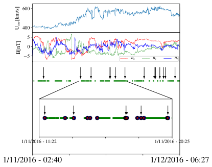
Figure 1: A short time window of the January 2016 dataset ($\sim$ 2 days). The first two top panels display the solar wind bulk speed and magnetic field components. The green horizontal lines represent the duration of the reconstructed flux ropes, the red stars and the blue circles (clearly visible in the inset) are the start and end time of PVI events. The black arrows indicate locations of larger PVI values.

4 Results

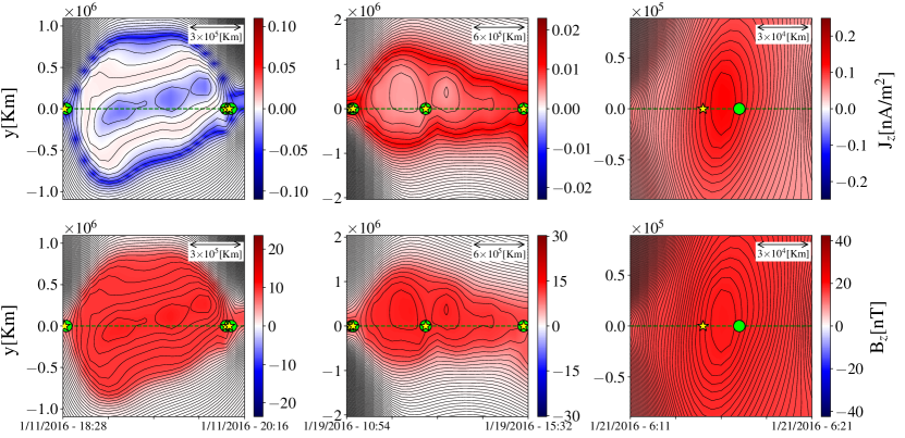
Figure 2: Reconstructed flux ropes for Wind January 2016 in the local frame (x,y), with the z-axis representing the cylindrical axis of the flux rope. Magnetic potential contour lines with filled color plots of $J_{z}[\mbox{A/m${}^{2}$}]$ (top panels) and $B_{z}[\mbox{nT}]$ (bottom panels). The dashed lines at $y=0$ are the projection of the spacecraft path on the flux rope cross section. The yellow stars and the green circles represent the start and the end time of the PVI events respectively. The distances in the transverse directions are in km, and they may be considered directly proportional to the magnetic flux across the flux rope. The x-axis of the figures represent the observation period, that we transformed into spatial dimensions (see the ruler inside the plots) applying Taylor hypothesis.

We employ in situ measurements of the interplanetary magnetic field and plasma parameters from the Wind spacecraft. Specifically for January 2016, we use the one-minute cadence data sets from the Magnetic Field Investigation (MFI) (Lepping et al., 1995) and the Solar Wind Experiment (SWE) (Ogilvie et al., 1995) instruments. All data are accessed via the NASA Coordinated Data Analysis Web (CDAWeb). For this period, we obtained $\sim 400$ magnetic islands or flux tube cross sections via the GS reconstruction and $\sim 400$ PVI events, calculated with a time lag $\tau=2$ min, applying a threshold on the PVI signal $\theta\sim 3.7$. The average that appears in the denominator of Equation 2 has been computed over the whole data set (Servidio et al., 2011). In Figure 1 we show an example of how the PVI and the GS methods work in synergy. The plot is a 1-dimensional view of about 2 day data, indicating the occurrence of flux ropes, with PVI events interposed, along with solar wind bulk speed and magnetic field components in the same period. The arrows point at the more extreme PVI events that clearly appear at the borders of the magnetic islands. The inset provides an expanded view of a shorter period of about 9 hours. The requirements coming for applicability of the GS equations in effect select time intervals during which a possible flux rope appears. In appropriate cases, we can improve our understanding of the magnetic field topology through GS reconstruction, which provides plausible 2D cross-sections of nearby magnetic islands. Meanwhile, the PVI method selects intervals that are suggestive of strong currents, which could be cores, but for very strong cases tend to be current sheets. Applying both methods simultaneously enables plausible identification of both flux tubes and coherent current structures at their boundaries and it can be done in any single (or multiple)-spacecraft measurement. Some examples of reconstructed flux ropes in 2D boxes (21$\times$141 points) and magnetic structures detected with the PVI method are shown in Figure 2, extracted from the same month of analyzed Wind data. The cross sections of the flux ropes are represented in the local reconstruction frame ($x$, $y$, $z$), with the $z$-axis pointing arbitrarily in space, representing the cylindrical axis of the flux rope.

Three cases are shown:
(I) The leftmost panels display current sheets localized at the borders of a large magnetic island, probably X points. The lateral extent of this island is of the order of 2 $\times$10⁶ km. Its z-axis is mainly in the GSE x-y plane. (II) In the middle panels a longer interval, corresponding to a span of about 5 nominal correlation scales, is shown. Within this very large structure, we find two PVI events near the left border of the island and one PVI event within. The latter can be interpreted as a core current, however, it is located between two secondary islands showing the complexity of the magnetic field texture. Here, the local z and GSE z-axes almost coincide. (III) The rightmost panels show a PVI event found within a magnetic island, where the value of $B_{z}$ is larger. This is probably a current sheet internal to the flux tube, associated with bunching of magnetic flux near the central axis which is an O point. This flux tube is smaller, about 3 $\times$10⁴ km across, or somewhat less than the average interplanetary correlation scale. In this case the axis of the flux rope points along the GSE y-axis. In the GS method, the boundaries of a given flux tube are determined by the requirement that the pressure-magnetic flux relation $P_{t}(A)$ remains single-valued, and the boundaries appear at points beyond which this can no longer be satisfied. In contrast, the PVI method identifies a current sheet boundary as a local condition on the vector increment. The boundaries are therefore determined independently in the two cases, and the finding that they frequently occur in the same or similar positions (see Figure 1 and Figure 2) indicates a synergy in the use of the combined GS/PVI method. In some reconstructed islands, we were not able to classify the PVI events either as X or as O points, and we called them neither (N) events. One explanation for these could be that the spacecraft moving in the solar wind may not come directly across the X or O points. One should be cognizant of the fact that current sheets in weakly three dimensional turbulence (Wan et al., 2014) may also appear within flux tubes but separated both from the magnetic axis (core) and the X-points that may be found at the boundary with other flux tubes. We are not aware that such current configurations have been reported as emerging in the purely 2D geometry assumed in the GS method. Evidently at least an elevation to a weakly 3D reduced MHD model is required (Rappazzo & Velli, 2011; Wan et al., 2014). Nevertheless, the GS method may detect signatures of such currents in the solar wind, even if this cannot emerge in a purely 2D dynamical model. The reconstruction method assumes a local 2D geometry that is organized by a strong local, out of plane guide field $B_{z}$ (Oughton et al., 1994, 2015), this state characterized by spatial derivatives along the $z$ direction that are weak relative to those computed in the perpendicular plane. Consequently, a measure of the goodness of the reconstruction may be given as the quantity $\mathcal{A}=\sqrt{\langle\mathbf{B}_{\perp}^{2}\rangle}/{B_{z}}$ where the averaging operation $\langle\dots\rangle$ is made over a moving window. By requiring that this quantity is less than $1$ we may exclude some reconstructed flux ropes and retain more trustworthy ones. Typical values of are of $A$ the order of $0.1$-$0.2$ for the “good cases”. However, in a few cases one finds values of $A$ around $0.6$-$0.8$ even if when reconstruction of the flux rope is very good. At this point, it is interesting to examine statistics of the location of the PVI events with respect to the magnetic islands. For example, are the more intense current sheets occurring at the boundaries of the islands (X points)? The statistical analysis of over $\sim 150$ refined events is shown in Figure 3. The histogram confirms that the events with the highest PVI values are located at the borders of the magnetic islands (where one expects tangential discontinuities and possible X points), whereas, the cores of the flux ropes (O points) are characterized by a broad range of PVI values. The unclassified events are a few percentages and at relatively small PVI values. These may be propagating (Wan et al., 2014) and are perhaps, more likely, rotational discontinuities. This observational evidence is in agreement with the numerical results obtained from a 2D compressible MHD simulation shown in Greco et al. (2009). A physically appealing interpretation emerged: very low values of current lie mainly in wide regions (lanes) among magnetic islands. These are associated with local low nonlinearity, and possibly wave-like activity (Howes et al., 2018) and other transient random currents (Greco et al., 2016; Franci et al., 2017). Current cores, required by Ampere’s law for any flux tube carrying non-zero current, populate the central regions of the magnetic islands (or flux tubes). And finally, small-scale current sheet-like structures form narrow regions (sharp boundaries) between magnetic islands. The current sheets represent the well-known small-scale coherent structures of MHD turbulence (Matthaeus & Montgomery, 1980; Veltri, 1999; Servidio et al., 2008), that are linked to the magnetic field intermittency. This classification provides a real-space picture of the nature of intermittent MHD turbulence and it found confirmation in the observational data.

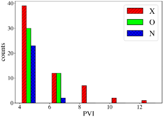
Figure 3: Histograms of PVI events classified as X points (striped red), O points (plain green) and N points (crossed blue). The histogram bins have the same width equal to $2$, starting from PVI$=3.7$.

We now turn to a comparison of the electric current densities implied by the GS method and the PVI method. The GS method, within the parameters of its approximations, returns directly, and at each point, a value of the current density. For the PVI method, we can use the empirical result in Fig. (7) of Greco et al. (2018) as a basis for estimation of the current in the sharp boundaries. The quoted result demonstrates a statistical relationship between the normalized current density, estimated with the curlometer technique (Dunlop et al., 2002), and the multi-spacecraft PVI index computed from MMS measurements in Earth’s magnetosheath. The relationship is found employing normalization of the current by $\sigma$, its root mean square value, a procedure needed to compare current measurements with PVI, a non-dimensional quantity. What is suggested in Greco et al. (2018) is a strong correlation between PVI and current density values that can be expressed as

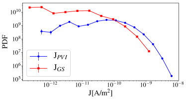
Figure 4: Probability Density Function of the current density evaluated with the GS method (red line) and from PVI signal (blue line).

$$\frac{\mbox{J}}{\sigma}\simeq 2\mbox{ PVI}.$$ (3)

Let us suppose that this statistical relationship applies to the WIND data in the solar wind, so we can use 3 to obtain a measure of J. To be useful, this procedure requires obtaining or estimating the value of $\sigma$ in the absence of a direct measure of current. (otherwise one would not need to use the relation 3). A reasonable estimate of $\sigma$ may be obtained based on computing the root mean square (RMS) value of the (single-spacecraft) measured vector magnetic field increments $|\Delta\bf B|$. To convert this value to units of current, one divides by the magnetic permeability $\mu_{0}$ and a length L$\sim 10^{4}$ km, that may be the typical scale of the current sheets. This estimate comes from the statistical distribution of PVI event duration multiplied by the solar wind speed and it is consistent with existing values in literature (e.g. Gosling & Szabo (2008)). In this approximation $\sigma\mbox{(A/m${}^{2}$)}=\mbox{RMS}(|\Delta{\bf B}|)/(\mbox{L}\mu_{0})$, where the average has been computed over the whole data set. Having $\sigma$ ($\sim 15\times 10^{-11}$ A/m²) and the entire PVI signal, J values come from the empirical expression 3

$$\mbox{J}_{PVI}~{}(\mbox{A/m}^{2})\sim 2\mbox{ PVI }\sigma~{}(\mbox{A/m}^{2}).$$ (4)

The numbers for current density obtained in this way may be compared and contrasted with the current obtained, that is implied, from the GS reconstruction, say $\mbox{J}_{GS}$, within each flux rope, sampled along the spacecraft path $(y=0)$. Accordingly, we compute the probability density functions (PDFs) of $\mbox{J}_{PVI}$ and $\mbox{J}_{GS}$ using these two methods and illustrate the corresponding distributions in Figure 4. We emphasize that the currents computed from the two methods are not expected to agree, given that the GS current is effectively based on the island cores while the PVI value is based on the boundaries. Indeed the figure shows that the $\mbox{J}_{PVI}$ distribution is displaced toward considerably larger value than the $\mbox{J}_{GS}$ distribution. The most probable GS current occurs at a value that is about two orders of magnitude smaller than the most probably PVI current. The PVI current distribution also exhibits a noticeable extended tail at large values.

5 Discussion

The GS reconstruction method and the PVI method provide complementary information when implemented together with a single-spacecraft time record of magnetic field. The results shown here demonstrate this synergy with regard to the overall flux tube structure that is revealed when both methods are employed: The GS method is sensitive to the large scale magnetic flux tube structure, i.e. the core currents and O-points, but is not very sensitive to the sharp boundaries, the mostly boundary current sheets and X-points. The PVI method has the opposite sensitivity, providing principally information about localized structures that contribute to intermittency, i.e., the flux tube boundaries and associated current sheets. The two methods identify structure boundaries independently so the result of this procedure provides a reasonable, if not purely rigorous, interpretation of the local topology of the magnetic field in the region threaded by the observed data. Another issue is the estimation of electric current density. This is typically measured in closely spaced multi-spacecraft missions employing a curlometer technique (Dunlop et al., 2002), for example in the Cluster and Magnetospheric Multiscale (MMS) missions. Curlometer is unavailable with single-spacecraft, and only with highly sensitive instruments such as MMS/FPI (Fast Plasma Investigation instrument) it is possible to have direct measurement of current density based on the difference in proton/ion and electron speeds (Pollock et al., 2016). However, using the present methods one may estimate currents based on these combined approaches: GS reconstruction provides a 2D picture of the weaker flux tube core currents, while the PVI technique along with a variance of increments affords an estimation of the most intense currents at coherent structures. We have demonstrated the combined GS/PVI method and provided additional observational evidence that observed solar wind discontinuities are coherent structures associated with the interaction of adjacent magnetic flux tubes (Greco et al., 2008). In particular, this type of strong current structure at small scales is readily interpreted as a consequence of the intermittent nature of fully developed MHD turbulence. (Matthaeus et al., 2015) The present analysis examines and supports the idea that the solar-wind plasma is structured (Schatten, 1971; Bruno et al., 2001; Borovsky, 2008), in the sense that flux tubes are filamentary or “spaghetti-like” (indeed Hu et al. (2018) found that the $\hat{z}$ axis of flux ropes at 1AU tend to be aligned with the Parker spiral direction), due to dynamical activity in the corona or in interplanetary space. With moderate to strong axial fields, it is widely acknowledged that the plasma tends to become locally quasi two dimensional (Matthaeus et al., 1990; Bieber et al., 1996; Hamilton et al., 2008; MacBride et al., 2010; Narita et al., 2010; Chen et al., 2012). Fast local relaxation (Servidio et al., 2008) also favors the 2D quasi-static approximation we employed. The presence of discontinuities or coherent current sheets that form between these magnetic flux tubes suggests nevertheless ongoing dynamical activity, and a subset of these might involve magnetic reconnection (Dmitruk & Matthaeus, 2006; Servidio et al., 2011). These structured flux tubes also provide conduits for energetic particle transport and possible trapping (Tessein et al., 2013; Khabarova et al., 2016; Pecora et al., 2018) and acceleration. Indeed one may envision numerous applications in which the combined GS/PVI method may reveal structures relevant to understand complex physics and turbulent interplanetary dynamics. The method may be particularly useful for revealing such features for Parker Solar Probe and Solar Orbiter missions, as they explore new regions of the heliosphere in which there are few established expectations for the nature of the magnetic field.

References

- Bieber et al. (1996) Bieber, J. W., Wanner, W., & Matthaeus, W. H. 1996, Journal of Geophysical Research: Space Physics, 101, 2511
- Borovsky (2008) Borovsky, J. E. 2008, Journal of Geophysical Research (Space Physics), 113, A08110
- Bruno et al. (1999) Bruno, R., Bavassano, B., Bianchini, L., et al. 1999, in ESA Special Publication, Vol. 9, Magnetic Fields and Solar Processes, ed. A. Wilson & et al., 1147
- Bruno & Carbone (2005) Bruno, R., & Carbone, V. 2005, Living Reviews in Solar Physics, 2, 4
- Bruno et al. (2001) Bruno, R., Carbone, V., Veltri, P., Pietropaolo, E., & Bavassano, B. 2001, Planet. Space Sci., 49, 1201
- Cartwright & Moldwin (2010) Cartwright, M. L., & Moldwin, M. B. 2010, Journal of Geophysical Research (Space Physics), 115, A08102
- Chen et al. (2012) Chen, C. H. K., Mallet, A., Schekochihin, A. A., et al. 2012, ApJ, 758, 120
- Chhiber et al. (2018) Chhiber, R., Chasapis, A., Bandyopadhyay, R., et al. 2018, Journal of Geophysical Research (Space Physics), 123, 9941
- De Hoffmann & Teller (1950) De Hoffmann, F., & Teller, E. 1950, Phys. Rev., 80, 692. https://link.aps.org/doi/10.1103/PhysRev.80.692
- Dmitruk & Matthaeus (2006) Dmitruk, P., & Matthaeus, W. H. 2006, Physics of Plasmas, 13, 042307
- Dunlop et al. (2002) Dunlop, M., Balogh, A., Glassmeier, K.-H., & Robert, P. 2002, Journal of Geophysical Research: Space Physics, 107, SMP
- Feng et al. (2008) Feng, H. Q., Wu, D. J., Lin, C. C., et al. 2008, Journal of Geophysical Research (Space Physics), 113, A12105
- Franci et al. (2017) Franci, L., Cerri, S. S., Califano, F., et al. 2017, ApJ, 850, L16
- Glassmeier et al. (2001) Glassmeier, K. H., Motschmann, U., Dunlop, M., et al. 2001, Annales Geophysicae, 19, 1439
- Goldstein et al. (1995) Goldstein, M. L., Roberts, D. A., & Matthaeus, W. H. 1995, ARA&A, 33, 283
- Gosling & Szabo (2008) Gosling, J., & Szabo, A. 2008, Journal of Geophysical Research: Space Physics, 113
- Gosling et al. (2011) Gosling, J., Tian, H., & Phan, T. 2011, The Astrophysical Journal Letters, 737, L35
- Greco et al. (2008) Greco, A., Chuychai, P., Matthaeus, W. H., Servidio, S., & Dmitruk, P. 2008, Geophys. Res. Lett., 35, L19111
- Greco et al. (2018) Greco, A., Matthaeus, W., Perri, S., et al. 2018, Space Science Reviews, 214, 1
- Greco et al. (2009) Greco, A., Matthaeus, W. H., Servidio, S., Chuychai, P., & Dmitruk, P. 2009, The Astrophysical Journall, 691, L111
- Greco et al. (2016) Greco, A., Perri, S., Servidio, S., Yordanova, E., & Veltri, P. 2016, ApJ, 823, L39
- Hamilton et al. (2008) Hamilton, K., Smith, C. W., Vasquez, B. J., & Leamon, R. J. 2008, Journal of Geophysical Research: Space Physics, 113
- Hasegawa et al. (2019) Hasegawa, H., Denton, R. E., Nakamura, R., et al. 2019, Journal of Geophysical Research (Space Physics), 124, 122
- Hau & Sonnerup (1999) Hau, L.-N., & Sonnerup, B. U. Ö. 1999, J. Geophys. Res., 104, 6899
- Howes et al. (2018) Howes, G. G., McCubbin, A. J., & Klein, K. G. 2018, Journal of Plasma Physics, 84, 905840105
- Hu (2017) Hu, Q. 2017, Sci. China Earth Sciences, 60, 1466
- Hu & Sonnerup (2002) Hu, Q., & Sonnerup, B. U. 2002, Journal of Geophysical Research: Space Physics, 107, SSH
- Hu et al. (2018) Hu, Q., Zheng, J., Chen, Y., le Roux, J., & Zhao, L. 2018, ApJS, 239, 12
- Khabarova et al. (2016) Khabarova, O. V., Zank, G. P., Li, G., et al. 2016, The Astrophysical Journal, 827, 122
- Kraichnan & Panda (1988) Kraichnan, R. H., & Panda, R. 1988, The Physics of fluids, 31, 2395
- Lepping et al. (1995) Lepping, R. P., Acũna, M. H., Burlaga, L. F., et al. 1995, Space Sci. Rev., 71, 207
- MacBride et al. (2010) MacBride, B. T., Smith, C. W., & Vasquez, B. J. 2010, Journal of Geophysical Research: Space Physics, 115
- Matthaeus et al. (1990) Matthaeus, W. H., Goldstein, M. L., & Roberts, D. A. 1990, Journal of Geophysical Research: Space Physics, 95, 20673
- Matthaeus & Montgomery (1980) Matthaeus, W. H., & Montgomery, D. 1980, Annals of the New York Academy of Sciences, 357, 203
- Matthaeus et al. (2016) Matthaeus, W. H., Parashar, T. N., Wan, M., & Wu, P. 2016, ApJ, 827, L7
- Matthaeus & Velli (2011) Matthaeus, W. H., & Velli, M. 2011, Space Sci. Rev., 160, 145
- Matthaeus et al. (2015) Matthaeus, W. H., Wan, M., Servidio, S., et al. 2015, Philosophical Transactions of the Royal Society A: Mathematical, Physical and Engineering Sciences, 373, 20140154
- Moldwin et al. (2000) Moldwin, M. B., Ford, S., Lepping, R., Slavin, J., & Szabo, A. 2000, Geophys. Res. Lett., 27, 57
- Moldwin et al. (1995) Moldwin, M. B., Phillips, J. L., Gosling, J. T., et al. 1995, J. Geophys. Res., 100, 19903
- Narita et al. (2010) Narita, Y., Glassmeier, K. H., Sahraoui, F., & Goldstein, M. L. 2010, Phys. Rev. Lett., 104, 171101
- Ogilvie et al. (1995) Ogilvie, K. W., Chornay, D. J., Fritzenreiter, R. J., et al. 1995, Space Sci. Rev., 71, 55
- Osman et al. (2014) Osman, K., Matthaeus, W., Gosling, J., et al. 2014, Physical Review Letters, 112, 215002
- Osman et al. (2011) Osman, K. T., Wan, M., Matthaeus, W. H., Breech, B., & Oughton, S. 2011, The Astrophysical Journal, 741, 75
- Oughton et al. (2015) Oughton, S., Matthaeus, W., Wan, M., & Osman, K. 2015, Philosophical Transactions of the Royal Society A: Mathematical, Physical and Engineering Sciences, 373, 20140152
- Oughton et al. (1994) Oughton, S., Priest, E. R., & Matthaeus, W. H. 1994, Journal of Fluid Mechanics, 280, 95
- Pecora et al. (2018) Pecora, F., Servidio, S., Greco, A., et al. 2018, Journal of Plasma Physics, 84, 725840601
- Pollock et al. (2016) Pollock, C., Moore, T., Jacques, A., et al. 2016, Space Science Reviews, 199, 331
- Rappazzo & Velli (2011) Rappazzo, A., & Velli, M. 2011, Physical Review E, 83, 065401
- Schatten (1971) Schatten, K. H. 1971, Reviews of Geophysics and Space Physics, 9, 773
- Servidio et al. (2011) Servidio, S., Greco, A., Matthaeus, W. H., Osman, K. T., & Dmitruk, P. 2011, Journal of Geophysical Research (Space Physics), 116, A09102
- Servidio et al. (2008) Servidio, S., Matthaeus, W., & Dmitruk, P. 2008, Physical review letters, 100, 095005
- Servidio et al. (2008) Servidio, S., Primavera, L., Carbone, V., Noullez, A., & Rypdal, K. 2008, Physics of Plasmas, 15, 012301
- Servidio et al. (2012) Servidio, S., Valentini, F., Califano, F., & Veltri, P. 2012, Physical review letters, 108, 045001
- Servidio et al. (2011) Servidio, S., Dmitruk, P., Greco, A., et al. 2011, Nonlinear Processes in Geophysics, 18, 675
- Shebalin et al. (1983) Shebalin, J. V., Matthaeus, W. H., & Montgomery, D. 1983, Journal of Plasma Physics, 29, 525
- Sonnerup & Guo (1996) Sonnerup, B. U. Ö., & Guo, M. 1996, Geophys. Res. Lett., 23, 3679
- Sonnerup et al. (2016) Sonnerup, B. U. Ö., Hasegawa, H., Denton, R. E., & Nakamura, T. K. M. 2016, Journal of Geophysical Research (Space Physics), 121, 4279
- Stribling & Matthaeus (1991) Stribling, T., & Matthaeus, W. H. 1991, Physics of Fluids B: Plasma Physics, 3, 1848
- Taylor (1974) Taylor, J. B. 1974, Physical Review Letters, 33, 1139
- Teh et al. (2010) Teh, W.-L., Sonnerup, B. U. Ö., Birn, J., & Denton, R. E. 2010, Annales Geophysicae, 28, 2113
- Tessein et al. (2013) Tessein, J. A., Matthaeus, W. H., Wan, M., et al. 2013, The Astrophysical Journall, 776, L8
- Veltri (1999) Veltri, P. 1999, Plasma Physics and Controlled Fusion, 41, A787
- Wan et al. (2014) Wan, M., Rappazzo, A. F., Matthaeus, W. H., Servidio, S., & Oughton, S. 2014, The Astrophysical Journal, 797, 63
- Yu et al. (2014) Yu, W., Farrugia, C. J., Lugaz, N., et al. 2014, AGU Fall Meeting Abstracts, SH31A