Mapping collinear in-medium parton splittings

Abstract

We map the spectrum of $1\to 2$ parton splittings inside a medium characterized by a transport coefficient $\hat{q}$ onto the kinematical Lund plane, taking into account the finite formation time of the process. We discuss the distinct regimes arising in this map for in-medium splittings, pointing out the close correspondence to a semi-classical description in the limit of hard, collinear radiation with short formation times. Although we disregard any modifications of the original parton kinematics in course of the propagation through the medium, subtle modifications to the radiation pattern compared to the vacuum baseline can be traced back to the physics of color decoherence and accumulated interactions in the medium. We provide theoretical support to vacuum-like emissions inside the medium by delimiting the regions of phase space where it is dominant, identifying also the relevant time-scales involved. The observed modifications are shown to be quite general for any dipole created in the medium.

1 Introduction

Jet quenching, the modification of jet observables in the presence of a QCD medium, is arguably the most versatile experimental tool to characterize the hot and dense system created in heavy-ion collisions, see e.g. [1, 2, 3]. In the last 20 years experiments at RHIC [4, 5] and then the LHC [6, 7, 8, 9, 10] found a strong suppression of particles produced at high transverse momentum, the most direct predictions of energy loss, one of the clearest signatures of the presence of jet quenching dynamics. The large kinematical reach of the LHC, and the much larger integrated luminosities expected for the near future, allow to adapt and design completely new jet tools [11, 12], originally developed for the proton-proton program, with a much more differential access to different properties of the medium. Two examples are the access to different energy scales in the medium properties, notably, the access to short distances to measure the properties of its quasiparticle content [13] and the access to the space-time evolution of the whole system [14], including its initial stages [15]. One essential ingredient for a correct interpretation of the data is a good control of the splitting process in the relevant energy- or time-scale under investigation. Interestingly, the new jet tools mentioned above can be used to isolate, or at least make it cleaner, these different scales [16].

The problem of elementary parton splittings is important in many aspects of high-energy physics. Most prominently, it allows to resum final-state emissions that accompany hard processes at colliders (a similar framework exists for resummation of initial-state radiation, but here we focus on the former). This is manifested experimentally as sprays of collimated particles, i.e. a jet. The fundamental splitting vertices together with a calculation of the available phase space are the ingredients that enter the formulation of a Monte Carlo parton shower.

For processes involving soft gluon radiation, one often invokes a strong separation of scales that allows to define a classical current. In a diagrammatic language, the current represents high-energy particles that act as sources of soft gluons and originate from a espacial position that is fixed in both the amplitude and its complex conjugate. This method has been shown to provide an economical description of both initial- and final-state emissions in the presence of a nuclear medium, e.g. see [17]. Similarly, the interference pattern off multiple emitters was studied assuming an instantaneous splitting of the current, giving rise to the so-called antenna radiation pattern [18, 19, 20, 21]. This picture was further corroborated within a diagrammatic calculation of the two-gluon emission spectrum in the limit of strong ordering of their respective emission times [22]. Recently, both Monte-Carlo studies [23, 24] and analytical calculations [25, 26], have highlighted the role of jet fluctuations that arise from in-medium splittings on observables that are sensitive to energy loss in heavy-ion collisions.

In this work we compute, within a diagrammatic approach, a real and collinear parton splitting inside a color deconfined medium and study the set of medium-induced modifications that arise from allowing this splitting to occur at a finite distance within the medium. Our discussion is most clearly cast in the context of a final-state color-singlet splitting, i.e. $\gamma\to q\bar{q}$, but remains valid for generic splitting processes involving a total color charge. We systematically implement the high-energy limit in our calculations, that reduces the complexity of the problem to a semi-classical picture of partons propagating along well-defined trajectories. Although we disregard any modifications of the original parton kinematics in course of the propagation through the medium, subtle modifications to the radiation pattern compared to the vacuum baseline can be traced back to the impact of physical time-scales in the medium, related to color decoherence and broadening.

The time-like separation of the splitting vertices in, respectively, the amplitude and the complex-conjugate amplitude gives rise to two- (dipole) and four-point (quadrupole) correlators of Wilson lines that resum medium interactions. These correspond to the survival probabilities of the two- and four-parton configurations at various stages of the process under consideration. It is crucial to note that in the absence of this separation these correlators collapse to unity, leaving no imprint on the splitting process. The appearance of the quadrupole, describing the propagation of the pair from formation time to the end of the medium, is essential since it accounts for the accumulated effects of medium interactions over long distances.

Let us also clarify what we mean by the decoherence of the dipole. In earlier works, where the dipole was assumed to form quasi-instantaneously close to the origin, color decoherence was shown to introduce a new timescale that governs the spectrum of subsequent soft emissions [19, 21, 20]. This comes about because the interference pattern between the radiation off each of the dipole constituents depends on the color coherence of the pair. In the current setup, we study in detail the formation of the dipole itself, for the moment without considering further radiative processes and ask the simple question of when and how such dipoles are formed. An important property to understand in this context is the locality of the splitting, i.e. whether the properties of the parton pair are determined at the moment of formation or whether those still can undergo modifications over large distances in the medium. Our results point to the importance of both regimes and quantify them in terms of logarithmic phase space. In close analogy to studies of dipole radiation patterns in vacuum, it is very helpful to map the kinematics of the formed dipoles onto the kinematical Lund plane [27]. Filling the Lund plane using jet de-clustering techniques in proton-proton and heavy-ion collisions has recently attracted a lot of attention [16, 28, 29, 30, 31].

Our final results for the emission spectrum in the presence of a medium can be cast in the form,

$${\frac{{\rm d}N^{\text{med}}}{{\rm d}z\,{\rm d}\theta}}\bigg{/}{\frac{{\rm d}N^{\text{vac}}}{{\rm d}z\,{\rm d}\theta}}=1+F_{\text{med}}\,,$$ (1)

where we have explicitly factorized the medium-induced cross-section into the vacuum cross-section and the medium-induced modification. The function $F_{\text{med}}$ encodes all information relative to the medium modification factor associated with the parton $1\to 2$ splitting function. We discuss the relevant approximations in the high-energy limit that allow to simplify the description in Sec.​ 2 and derive this expression in Sec.​ 3. In practice, this factorization allows for the straightforward discrimination of medium effects, as will be fully explained in Sec.​ 3. We discuss the relevant time-scales contained in the spectrum in Sec.​ 4 and draw the phase space for the process under consideration in Sec.​ 5. Then, in Sec.​ 6, we discuss numerical results that largely verify the preceding analysis. The steps needed to generalize the process under consideration to be valid for arbitrary splitting processes, involving e.g. color-charged dipoles etc., are outlined in Sec.​ 7 and, finally, we present an outlook in Sec.​ 8.

2 Implementing the semi-classical limit

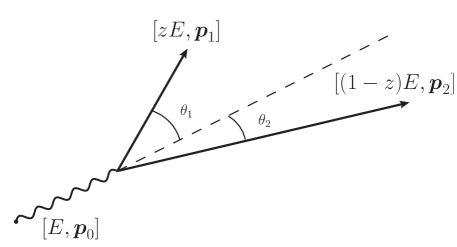
Figure 1: Kinematics of the parton splitting process. The dipole opening angle is ${\boldsymbol{n}}_{12}={\boldsymbol{n}}_{1}-{\boldsymbol{n}}_{2}$, with $|{\boldsymbol{n}}_{1}|=\theta_{1}$, $|{\boldsymbol{n}}_{2}|=\theta_{2}$ and $|{\boldsymbol{n}}_{12}|=\theta$.

Let us consider the splitting of a “parent” parton, with momentum $\vec{p}_{0}=[E,{\boldsymbol{p}}_{0}]$, into two “daughter” partons, with final-state kinematics

$$\vec{p}_{1}=[zE,{\boldsymbol{p}}_{1}]\,,\;\;\vec{p}_{2}=[(1-z)E,{\boldsymbol{p}}_{2}]\,,$$ (2)

where ${\boldsymbol{p}}_{0}={\boldsymbol{p}}_{1}+{\boldsymbol{p}}_{2}$ from conservation of transverse momentum. For the moment, we will focus on the production of a color singlet final-state, in particular the splitting of a photon into a quark-antiquark pair, $\gamma\to q\bar{q}$, where the photon is transversely polarized. This is illustrated in Fig.​ 1. The partial amplitude $\mathcal{M}$ for such a process, stripped of the Born-level production amplitude, reads (see also [32])

$$\mathcal{M}_{\gamma\rightarrow q\bar{q}} =\frac{e}{E}{\rm e}^{i\frac{{\boldsymbol{p}}_{1}^{2}}{2zE}L+i\frac{{\boldsymbol{p}}_{2}^{2}}{2(1-z)E}L}\int_{0}^{\infty}{\rm d}t\ \int_{{\boldsymbol{k}}_{1},{\boldsymbol{k}}_{2}}\left[\mathcal{G}({\boldsymbol{p}}_{1},L;{\boldsymbol{k}}_{1},t|zE)\,\mathcal{\bar{G}}({\boldsymbol{p}}_{2},L;{\boldsymbol{k}}_{2},t|(1-z)E)\right]_{ij}$$

$$\times\gamma_{\lambda,s,s^{\prime}}(z){\boldsymbol{k}}\cdot{\boldsymbol{\epsilon}}_{\lambda}^{\ast}\,\mathcal{G}_{0}({\boldsymbol{k}}_{1}+{\boldsymbol{k}}_{2},t|E)$$ (3)

where $e$ is the QED coupling constant and $\gamma_{\lambda,s,s^{\prime}}(z)=i\delta_{s,-s^{\prime}}[z\delta_{\lambda,s}-(1-z)\delta_{\lambda,-s}]/\sqrt{z(1-z)}$ is the quark-gluon splitting vertex with $\lambda=\pm 1$ and ${\boldsymbol{k}}\equiv(1-z){\boldsymbol{k}}_{1}-z{\boldsymbol{k}}_{2}$. Throughout, we implement the notations $\int_{{\boldsymbol{x}}}\equiv\int{\rm d}^{2}{\boldsymbol{x}}$ for transverse coordinate and $\int_{{\boldsymbol{k}}}\equiv\int{\rm d}^{2}{\boldsymbol{k}}/(2\pi)^{2}$ for transverse momentum integrations. In this expression, $\mathcal{G}$ and $\mathcal{\bar{G}}$ represent the dressed retarded propagators for the quark and the antiquark, that incorporate an adiabatic turn-off at large times, see e.g. [33] for details on this regulator. As usual for high-energy processes, we have assumed that interactions with the medium only exchange transverse momentum. Hence the momenta ${\boldsymbol{k}}_{1}$ and ${\boldsymbol{k}}_{2}$ correspond to the transverse momentum sharing immediately after splitting.

The fully dressed propagator in the momentum space transforms to configuration space according to,

$$\mathcal{G}({\boldsymbol{p}}_{1},t_{1};{\boldsymbol{p}}_{0},t_{0}) =\int_{{\boldsymbol{x}}_{1},{\boldsymbol{x}}_{2}}{\rm e}^{-i{\boldsymbol{p}}_{1}\cdot{\boldsymbol{x}}_{1}+i{\boldsymbol{p}}_{0}\cdot{\boldsymbol{x}}_{0}}\mathcal{G}(\vec{x}_{1},\vec{x}_{0})\,,$$ (4)

where we have suppressed the color and energy indices. In configuration space, $\mathcal{G}(\vec{x}_{1},\vec{x}_{0})$ is described by a 2+1 dimensional path integral along the trajectory of the particle,

$$\mathcal{G}(\vec{x}_{1},\vec{x}_{0})=\int_{{\boldsymbol{r}}(t_{0})={\boldsymbol{x}}_{0}}^{{\boldsymbol{r}}(t_{1})={\boldsymbol{x}}_{1}}\mathcal{D}{\boldsymbol{r}}\,\exp\left[i\frac{E}{2}\int_{t_{0}}^{t_{1}}{\rm d}s\,\dot{\boldsymbol{r}}^{2}\right]V(t_{1},t_{0};[{\boldsymbol{r}}])\,,$$ (5)

where the (conserved) energy $E$ acts as a “mass”. Here, $V(t_{1},t_{0};[{\boldsymbol{r}}])$ is a Wilson line in the fundamental representation at (possibly fluctuating transverse) position ${\boldsymbol{r}}(t)$,

$$V(t_{1},t_{0};[{\boldsymbol{r}}])=\mathcal{P}\exp\left[ig\int_{t_{0}}^{t_{1}}{\rm d}t\,\textbf{t}^{a}A^{-,a}(t,{\boldsymbol{r}}(t))\right],$$ (6)

where $\textbf{t}^{a}$ is a color matrix in the fundamental representation and $A^{-,a}(t,{\boldsymbol{r}})$ is a background field describing interactions with the medium. The antiquark propagator $\mathcal{\bar{G}}(\vec{x}_{1};\vec{x}_{0})$ is defined analogously to (5) with the substitution $V(t_{1},t_{0};[{\boldsymbol{r}}])\to V^{\dagger}(t_{1},t_{0};[{\boldsymbol{r}}])$. For propagation outside of the medium, these propagators reduce to

$$\mathcal{G}({\boldsymbol{p}}_{1},L;{\boldsymbol{k}}_{1},t|E)\big{|}_{t>L}=(2\pi)^{2}\delta({\boldsymbol{k}}_{1}-{\boldsymbol{p}}_{1})\,\mathcal{G}_{0}({\boldsymbol{p}}_{1},L-t|E)\,,$$ (7)

and analogously for $\mathcal{\bar{G}}$, where $\mathcal{G}_{0}({\boldsymbol{k}},t|E)={\rm e}^{-i\frac{{\boldsymbol{k}}^{2}}{2E}t}$. This corresponds also to the photon propagator in Eq. (2).

The goal of this work is to focus on the limit of hard splittings in the medium, i.e. splittings with formation times much shorter than the typical time-scales of the medium, where we expect a “semi-classical” picture to dominate the cross section. We make this statement more precise and map out the relevant region in phase space in Sec.​ 4 and Sec.​ 5. This is in contrast to the limit of medium-induced branching [34, 35, 33, 36, 37, 38, 39, 40, 41], where one investigates emissions with transverse momenta dominated by interactions with the medium, i.e. $p_{\perp}\sim\sqrt{\hat{q}zE}$. We will work in the high-energy limit, i.e. where formally the energy of the particles is infinite, $E\to\infty$, but we will keep track of the finite momentum sharing fraction $z$. It turns out that we need to consider two separate steps in order to establish this correspondence, which we proceed to outline below. The first step fixes the trajectories of the particles to follow classical trajectories that are determined by the kinematics of the process while the second one fixes a common reference point for the pair in transverse coordinates.

By hard emissions, we explicitly mean that both partons have energy large enough so that the change in transverse position due to scattering with the medium can be neglected and the propagation follows basically straight lines. This contribution can be isolated by considering the so-called eikonal expansion of the propagator (5) [42, 43]. Its zeroth-order term, which neglects further transverse momentum broadening in the medium, turns out to be

$$\mathcal{G}^{(0)}(\vec{x}_{1},\vec{x}_{0})=\mathcal{G}_{0}({\boldsymbol{x}}_{1}-{\boldsymbol{x}}_{0},t_{1}-t_{0})V(t_{1},t_{0};[{\boldsymbol{x}}_{\rm cl}])\,,$$ (8)

where ${\boldsymbol{x}}_{\rm cl}(t)=\frac{t_{1}-t}{t_{1}-t_{0}}{\boldsymbol{x}}_{0}+\frac{t-t_{0}}{t_{1}-t_{0}}{\boldsymbol{x}}_{1}$ is the classical path. Taking the Fourier transform, see Eq. (4), and after some manipulations, we find that the propagator in mixed representation becomes

$$\mathcal{G}^{(0)}({\boldsymbol{p}}_{1},t_{1};{\boldsymbol{p}}_{0},t_{0}) ={\rm e}^{-i\frac{{\boldsymbol{p}}_{1}^{2}}{2E}(t_{1}-t_{0})}\int_{{\boldsymbol{y}}_{0},{\boldsymbol{y}}_{1}}\,{\rm e}^{-i({\boldsymbol{p}}_{1}-{\boldsymbol{p}}_{0})\cdot{\boldsymbol{y}}_{0}}\,\frac{E(t_{1}-t_{0})}{2\pi i}{\rm e}^{i\frac{E(t_{1}-t_{0})}{2}({\boldsymbol{y}}_{1}-{\boldsymbol{n}})^{2}}$$

$$\times V(t_{1},t_{0};[{\boldsymbol{y}}_{0}+(t-t_{0}){\boldsymbol{y}}_{1}])\,,$$ (9)

where ${\boldsymbol{n}}\equiv{\boldsymbol{p}}_{1}/E$. In the “semi-classical” limit $E(t_{1}-t_{0})\gg 1$ (corresponding to the formal limit $\hbar\to 0$) the heat-kernel in (2) reduces to a delta function of its argument, $\lim_{\varepsilon\to 0}{\rm e}^{-{\boldsymbol{x}}^{2}/\varepsilon}/(\pi\varepsilon)=\delta({\boldsymbol{x}})$. In particular, we demand that $E\gg L^{-1}$. This step converges the particles path onto the classical trajectory, and the propagator becomes

$$\mathcal{G}^{(0)}({\boldsymbol{p}}_{1},t_{1};{\boldsymbol{p}}_{0},t_{0})={\rm e}^{-i\frac{{\boldsymbol{p}}_{1}^{2}}{2E}(t_{1}-t_{0})}\int_{\boldsymbol{x}}\,{\rm e}^{-i({\boldsymbol{p}}_{1}-{\boldsymbol{p}}_{0})\cdot{\boldsymbol{x}}}V(t_{1},t_{0};[{\boldsymbol{x}}+(t-t_{0}){\boldsymbol{n}}])\,,$$ (10)

see also [44]. This expression corresponds to the S-matrix of an energetic particle that traverses the medium, see e.g. [45].

Hence, in this first step we have removed all effects of non-eikonal broadening in the medium, i.e. that associated to the fluctuations in the transverse position, after the pair has been created. However, the initial position of the trajectory of each leg is not fixed by (10). This leads to a “smearing” of the antenna initial position in transverse space. We will briefly return to this detail in A. For physical processes happening at large times from the initial position we can treat the initial position of the Wilson line as a small correction. Then we find

$$\mathcal{G}^{(0)}({\boldsymbol{p}}_{1},t_{1};{\boldsymbol{p}}_{0},t_{0})=(2\pi)^{2}\delta({\boldsymbol{p}}_{0}-{\boldsymbol{p}}_{1})\,{\rm e}^{-i\frac{{\boldsymbol{p}}_{1}^{2}}{2E}(t_{1}-t_{0})}V(t_{1},t_{0};\big{[}{\boldsymbol{n}}t\big{]})$$ (11)

for the quark propagator. This ensures that the Wilson lines accompanying the two hard particles always are initiated at the same initial transverse position and time.

Replacing the propagators in Eq. (2) with (11) and considering the splitting inside the medium, $0<t<L$, the amplitude becomes

$$\mathcal{M}^{\rm in}_{\gamma\rightarrow q\bar{q}}=\frac{e}{E}\gamma_{\lambda,s,s^{\prime}}(z)\,{\boldsymbol{p}}\cdot{\boldsymbol{\epsilon}}_{\lambda}^{\ast}\int_{0}^{L}{\rm d}t\,\exp\left(-i\frac{L-t}{{t_{\text{f}}}}\right)\Big{[}V_{1}(L,t)V^{\dagger}_{2}(L,t)\Big{]}_{ij},$$ (12)

where now ${\boldsymbol{p}}\equiv(1-z){\boldsymbol{p}}_{1}-z{\boldsymbol{p}}_{2}$ is only related to the final-state momenta. In this expression, we identify the quantum-mechanical formation time

$${t_{\text{f}}}=\frac{2z(1-z)E}{{\boldsymbol{p}}^{2}}\,.$$ (13)

This second step completes the semi-classical approximation where the particles are propagating along trajectories determined by their kinematics. The two Wilson lines are associated with each of the dipole constituents, such that e.g. $V_{i}(\bar{t},t)\equiv V(\bar{t},t;[{\boldsymbol{r}}_{i}(s)])$ with ${\boldsymbol{r}}_{i}(s)={\boldsymbol{n}}_{i}s$. Explicitly, ${\boldsymbol{n}}_{1}={\boldsymbol{p}}_{1}/[zE]$ and ${\boldsymbol{n}}_{2}={\boldsymbol{p}}_{2}/[(1-z)E]$. For emissions taking place outside of the medium, $t>L$, on the other hand, we can explicitly perform the integration over the splitting time. The amplitude reads then

$$\mathcal{M}^{\rm out}_{\gamma\to q\bar{q}}=\delta_{ij}\,\frac{i\,z(1-z)\,e}{E}\gamma_{\lambda,s,s^{\prime}}(z)\frac{{\boldsymbol{p}}\cdot\epsilon^{\ast}_{\lambda}}{{\boldsymbol{p}}^{2}},$$ (14)

where we have assumed the adiabatic turn-off prescription at large times mentioned above (consistent with the usual Feynman prescription in the vacuum propagators in momentum space). The amplitudes (12) and (14) are written up to pure phase factors that cancel out in the cross sections. The full amplitude is simply the sum $\mathcal{M}_{\gamma\to q\bar{q}}=\mathcal{M}^{\rm in}_{\gamma\to q\bar{q}}+\mathcal{M}^{\rm out}_{\gamma\to q\bar{q}}$.

3 Derivation of the spectrum

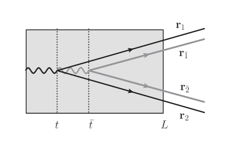
Figure 2: The “in-in” contribution to the spectrum. Amplitude (black lines) and complex conjugate of the amplitude (grey lines) are plotted on top of each other to clearly show the different contributions: dipole (15) in the region $(t,\bar{t})$ and quadrupole (16) in $(\bar{t},L)$.

Moving to the computation of the spectrum of splittings, the following definitions will become very helpful. We note that in our setup the trajectories of the particles in the amplitude, denoted by ${\boldsymbol{r}}_{1}$ and ${\boldsymbol{r}}_{2}$, and complex-conjugate amplitude, denoted ${\boldsymbol{r}}_{\bar{1}}$ and ${\boldsymbol{r}}_{\bar{2}}$, are shifted only due the difference in the splitting time which vary independently, see Fig.​ 2. The two-point function,

$$S_{\scriptscriptstyle IJ}(t_{1},t_{0})\equiv\frac{1}{N_{c}}\langle{\rm tr}\,V_{\scriptscriptstyle I}V^{\dagger}_{\scriptscriptstyle J}\rangle\,,$$ (15)

corresponds to the dipole cross section, where the extent of the Wilson lines is implicit from the left-hand side of the equation and $\{I,J\}=\{1,2,\bar{1},\bar{2}\}$. Finally, the four-point function,

$$Q(t_{1},t_{0})=\frac{1}{N_{c}}\langle{\rm tr}\,V_{1}V_{2}^{\dagger}V_{\bar{2}}V_{\bar{1}}^{\dagger}\rangle\,,$$ (16)

is also referred to as a quadrupole. In the harmonic oscillator approximation and in a static medium of size $L$, for details see [45],

$$S_{\scriptscriptstyle IJ}(t_{1},t_{0})=\exp\left[-\frac{1}{4}\hat{q}\int_{t_{0}}^{t_{1}}{\rm d}s\,{\boldsymbol{r}}^{2}_{\scriptscriptstyle IJ}(s)\right]\,,$$ (17)

where $\hat{q}\equiv C_{F}\hat{\overline{q}}$ is the transport coefficient for fundamental degrees of freedom and ${\boldsymbol{r}}_{\scriptscriptstyle IJ}\equiv{\boldsymbol{r}}_{\scriptscriptstyle I}-{\boldsymbol{r}}_{\scriptscriptstyle J}$ describes the separation of the Wilson lines in transverse coordinate. In the large-$N_{c}$ limit, the quadrupole can be written as [39, 40, 41],

$$Q(t_{1},t_{0})=S_{1\bar{1}}(t_{1},t_{0})S_{2\bar{2}}(t_{1},t_{0})+\int_{t_{0}}^{t_{1}}{\rm d}s\,S_{1\bar{1}}(t_{1},s)S_{2\bar{2}}(t_{1},s)\,T(s)\,S_{12}(s,t_{0})S_{\bar{1}\bar{2}}(s,t_{0})\,,$$ (18)

where $T(s)=-\hat{q}[{\boldsymbol{r}}_{12}^{2}(s)+{\boldsymbol{r}}_{\bar{1}\bar{2}}^{2}(s)-{\boldsymbol{r}}_{1\bar{2}}^{2}(s)-{\boldsymbol{r}}_{\bar{1}2}^{2}(s)]/2=-\hat{q}{\boldsymbol{r}}_{1\bar{1}}(s)\cdot{\boldsymbol{r}}_{2\bar{2}}(s)$ is the transition amplitude. Above, the two terms in (18) are the so-called factorizable and non-factorizable pieces of the quadrupole, and describe the propagation of two possible color configurations in the large-$N_{c}$ limit, under the constraint of conserving color at any given time. Concretely, the first term describes the propagation of two dipoles that correlate separately particle 1 and particle 2 in amplitude and complex conjugate (c.c.) amplitude so that they evolve independently. This is why this piece is called factorizable. The second, non-factorizable term involves a one-gluon exchange—described by the transition amplitude—that alters the color correlation of the system from an initial correlation of particles 1 and 2 in the amplitude and similarly in the c.c. at times $t<s$, to the uncorrelated case at times $t>s$.

Note that, for the problem at hand, the separations are either constant or grow linearly with time. In the high-energy limit, it is the separation of the splitting time in the amplitude $t$ and the splitting time in the c.c. amplitude $\bar{t}$ that govern the exact trajectories of the Wilson lines. For reference, we list the relevant differences here,

$${\boldsymbol{r}}_{1\bar{1}}(s) ={\boldsymbol{n}}_{1}(\bar{t}-t)\,,\;\;{\boldsymbol{r}}_{2\bar{2}}(s)={\boldsymbol{n}}_{2}(\bar{t}-t)\,,$$ (19)

$${\boldsymbol{r}}_{12}(s) ={\boldsymbol{n}}_{12}(s-t)\,,\;\;{\boldsymbol{r}}_{\bar{1}\bar{2}}(s)={\boldsymbol{n}}_{12}(s-\bar{t})\,,$$ (20)

where ${\boldsymbol{n}}_{12}\equiv{\boldsymbol{n}}_{1}-{\boldsymbol{n}}_{2}$. Note also that ${\boldsymbol{n}}_{12}={\boldsymbol{p}}/(z(1-z)E)$, where ${\boldsymbol{p}}=(1-z){\boldsymbol{p}}_{1}-z{\boldsymbol{p}}_{2}$ is the relative transverse momentum of the pair. Assuming a vanishing initial momentum ${\boldsymbol{p}}_{0}$, we can also deduce that ${\boldsymbol{n}}_{1}=(1-z){\boldsymbol{n}}_{12}$ and ${\boldsymbol{n}}_{2}=-z{\boldsymbol{n}}_{12}$, with $\theta\equiv|{\boldsymbol{n}}_{12}|$ and $\theta_{1(2)}\equiv|{\boldsymbol{n}}_{1(2)}|$, see Fig.​ 1. In this case, the transition amplitude takes the simple form

$$T(s)=-\hat{q}\,{\boldsymbol{n}}_{1}\cdot{\boldsymbol{n}}_{2}(\bar{t}-t)^{2}=-\hat{q}z(1-z){\boldsymbol{n}}_{12}^{2}(\bar{t}-t)^{2}.$$ (21)

For future reference, we take note that $\sum_{\lambda,s,s^{\prime}}|\gamma_{\lambda,s,s^{\prime}}(z)|^{2}=[z^{2}+(1-z)^{2}]/[z(1-z)]$.

The inclusive spectrum for the splitting process we are considering can be written as,

$$\frac{{\rm d}N^{\rm med}}{{\rm d}z{\rm d}{\boldsymbol{p}}^{2}}=\frac{1}{4(2\pi)^{2}\,z(1-z)}\langle\left|\mathcal{M}_{\gamma\to q\bar{q}}\right|^{2}\rangle=\frac{1}{4(2\pi)^{2}\,z(1-z)}\langle\left|\mathcal{M}_{\gamma\to q\bar{q}}^{\rm in}+\mathcal{M}_{\gamma\to q\bar{q}}^{\rm out}\right|^{2}\rangle\,,$$ (22)

where the averaging of the amplitude also takes into account averaging over the ensemble of medium configurations. The total spectrum in the presence of a medium can be decomposed into three parts, $N^{\rm med}=N^{\rm in-in}+N^{\rm in-out}+N^{\rm vac}$. Here, the first contribution corresponds to a splitting taking place inside the medium in both the amplitude and the c.c. amplitude, the second contribution is an interference between an emission taking place inside the medium in the amplitude and outside the medium in the c.c. amplitude, or vice versa, and the last term corresponds to an emission outside the medium. We define the vacuum cross-section from $\langle|\mathcal{M}^{\text{out}}|^{2}\rangle$. It reads,

$$\frac{{\rm d}N^{\text{vac}}}{{\rm d}z\,{\rm d}\theta}=\frac{\alpha_{\text{em}}}{\pi}\frac{P_{q\gamma}(z)}{\theta}\,,$$ (23)

where we used that ${\boldsymbol{p}}^{2}=[z(1-z)E\theta]^{2}$, $P_{q\gamma}(z)=n_{f}N_{c}[z^{2}+(1-z)^{2}]$ being the relevant Altarelli-Parisi splitting function and $n_{f}$ is the number of quark flavors. Then, after simplifying, we can write for the “in-in” spectrum

$$\frac{{\rm d}N^{\text{in-in}}}{{\rm d}z\,{\rm d}\theta} =\frac{{\rm d}N^{\text{vac}}}{{\rm d}z\,{\rm d}\theta}\;2{\rm Re}\int_{0}^{L}\frac{{\rm d}t}{{t_{\text{f}}}}\int_{t}^{L}\frac{{\rm d}\bar{t}}{{t_{\text{f}}}}\,{\rm e}^{-i\frac{\bar{t}-t}{{t_{\text{f}}}}}\,Q(L,\bar{t})S_{12}(\bar{t},t)\,,$$ (24)

where the quadrupole $Q(L,\bar{t})\equiv Q(L,\bar{t};t)$ explicitly depends on the splitting time in the amplitude through the finite longitudinal shift of the long-distance propagators. The in-out spectrum reads,

$$\frac{{\rm d}N^{\text{in-out}}}{{\rm d}z\,{\rm d}\theta}=-\frac{{\rm d}N^{\text{vac}}}{{\rm d}z\,{\rm d}\theta}\;2\text{Im}\int_{0}^{L}\frac{{\rm d}t}{{t_{\text{f}}}}\,{\rm e}^{-i\frac{L-t}{{t_{\text{f}}}}}\,S_{12}(L,t)\,.$$ (25)

Summing up all three contributions, the final spectrum takes the form

$$\frac{{\rm d}N^{\text{med}}}{{\rm d}z\,{\rm d}\theta}=\frac{{\rm d}N^{\text{vac}}}{{\rm d}z\,{\rm d}\theta}\,\big{(}1+F_{\text{med}}(z,\theta)\big{)}\,,$$ (26)

where the medium modifications are encoded in the factor $F_{\text{med}}$ that reads,

$$F_{\text{med}}=2\int^{L}_{0}\frac{{\rm d}t}{{t_{\text{f}}}}\left[\int^{L}_{t}\frac{{\rm d}\bar{t}}{{t_{\text{f}}}}\,\cos\left(\frac{\bar{t}-t}{{t_{\text{f}}}}\right)S_{12}(\bar{t},t)Q(L,\bar{t})-\sin\left(\frac{L-t}{{t_{\text{f}}}}\right)S_{12}(L,t)\right]\,,$$ (27)

with $S_{12}(\bar{t},t)\equiv S_{12}(\tau)$ and $Q(L,\bar{t})\equiv Q(\tau_{L},\tau)$ that only depend on the differences $\tau=\bar{t}-t$ and $\tau_{L}=L-\bar{t}$. Explicitly, these functions read

$$S_{12}(\tau) ={\rm e}^{-\frac{1}{12}\hat{q}\theta^{2}\tau^{3}}\,,$$ (28)

$$Q(\tau_{L},\tau) ={\rm e}^{-\frac{1}{4}\hat{q}\xi\theta^{2}\tau_{L}\tau^{2}}+T(\tau)\int^{L}_{\bar{t}}{\rm d}s\,{\rm e}^{-\frac{1}{4}\hat{q}\xi\theta^{2}(L-s)\tau^{2}}{\rm e}^{-\frac{1}{12}\hat{q}\theta^{2}[(s-\bar{t})^{3}+(s-t)^{3}-\tau^{3}]}\,,$$ (29)

where $s\geq\bar{t}\geq t$ and we defined $\xi=(1-z)^{2}+z^{2}$. The factorization property in Eq. (26) stems from the fact that the kinematics of the dipole is not modified after it has been created. In contrast, for medium-induced branching the daughter particles experience additional momentum broadening from to non-eikonal contributions both during their formation time and afterwards [39, 40, 41]. The dependence on the initial energy does not factorize completely on the right-hand-side of the equation due to the explicit dependence on the formation time ${t_{\text{f}}}$.

The process described by Eq. (27) contains two stages. To be accurate, for the in-out term, see (25), only the first stage plays a role. The first stage is governed by the dipole cross section $S_{12}(t_{1},t_{0})$ that appears in both terms in Eq. (27). It can be interpreted as a survival probability of a (virtual) dipole consisting of the daughter particles 1 and 2, with a dynamical transverse size $b_{\perp}(t)\sim\theta t$, that exist during the time interval $\Delta t=t_{1}-t_{0}$. We will refer to this stage of the process as the “decoherence” of the pair. The quadrupole $Q(\tau_{L},\tau)$ plays only a role for the “in-in” term, see Eq. (24). Looking in detail, the first term in (29) describes the survival probability of a (real) dipole with fixed transverse size $b_{\perp}\sim\theta\tau$ at the moment of formation, propagating the remaining distance to the end of the medium. Therefore, we will refer to this part of the dynamics as the broadening of the dipole. As mentioned before, in our approximation this broadening does not receive contributions from the non-eikonal fluctuations that change the transverse position of the propagating particles off their classical paths. The non-factorizable piece, given by the second term in Eq. (29), is typically a small correction. For example, the transition amplitude $T(\tau)\sim z\theta^{2}\tau^{2}$ becomes approximately $T(\tau)\sim{t_{\text{f}}}/E$ for short-formation times, i.e. when $\tau\sim{t_{\text{f}}}\ll L$ (see discussion in Sec.​ 4). It also vanishes in the soft limit $z\to 0$ and $\tau\sim$ const.

The terms in (27) correspond, respectively, to the cases when the splitting occurs inside the medium in both the amplitude and its complex conjugate, $\propto\langle|\mathcal{M}^{\text{in}}_{\gamma\to q\bar{q}}|^{2}\rangle$ (first term), already referred to as an “in-in” contribution, and the interference between a splitting inside and a splitting outside, $\propto 2{\rm Re}\langle\mathcal{M}^{\text{in}}_{\gamma\to q\bar{q}}\mathcal{M}^{{\dagger},\text{out}}_{\gamma\to q\bar{q}}\rangle$ (second term), analogously referred to as an “in-out” contribution. Keeping the size of the medium fixed $L=\text{const.}$ and reducing the medium density $\hat{q}\to 0$ reveals a non-trivial cancellation between the two terms that leads to $F_{\text{med}}\to 0$.

4 Qualitative discussion of scales

Presently, let us discuss the relevant scales that appear in the calculation. Considering (27), the emission process is characterized by a competition between the quantum mechanical formation process, that enforces $\tau\lesssim{t_{\text{f}}}$ for the “in-in” and $L-t\lesssim{t_{\text{f}}}$ for the “in-out” terms, respectively, as well as the suppression factors related to color decoherence and broadening. The condition on the splitting times is a consequence of avoiding strong oscillations of the trigonometric factors in (27).

The relevant scales for the “in-in” spectrum can be identified in the dipole and the factorizable piece of the quadrupole, i.e. the first term in (29). We will refer to them as the decoherence and broadening times, and they are given by

$$t_{\text{d}}\sim\left(\frac{1}{\hat{q}\theta^{2}}\right)^{1/3}\,,\qquad t_{\text{broad}}\sim\left(\frac{1}{\hat{q}\theta^{2}L}\right)^{1/2}\,.$$ (30)

The non-factorizable part of the quadrupole constitutes a small correction to this qualitative estimate. The decoherence time governs the color decoherence of a dipole, and for $t_{\text{d}}>L$, which implies that $\theta<\theta_{c}\sim(\hat{q}L^{3})^{-1/2}$, the survival probability is close to one. This means that the medium does not resolve the dipole until it exits the medium. In particular, ${t_{\text{f}}}<t_{\text{d}}$ implies that ${\boldsymbol{p}}^{2}>\sqrt{\hat{q}z(1-z)E}$, which is related to the transverse momentum broadening accumulated during the formation time. The broadening time scale, on the other hand, is related to transverse momentum broadening along the medium length $L$. The condition ${t_{\text{f}}}<t_{\text{broad}}$ implies that ${\boldsymbol{p}}^{2}>Q^{2}_{s}\sim\hat{q}L$. In the opposite case, the original opening angle of the dipole will be significantly changed by broadening, and the angle at which the particles emerge does not correspond to their initial opening angle. Note that $t_{\text{broad}}<t_{\text{d}}$ for $\theta>\theta_{c}$, which implies that the broadening along the whole medium length is typically larger than during the formation time of (relatively) large-angle splittings. Hence, for emissions with $\theta<\theta_{c}$ one should not expect any medium modifications, i.e. $F_{\text{med}}=0$. More importantly, the kinematical phase space for in-medium splittings that are vacuum-like, again implied by a vanishing $F_{\text{med}}$, also does exist for ${t_{\text{f}}}<t_{\text{broad}}<t_{\text{d}}$ at large angles $\theta>\theta_{c}$. We will compute the size of this phase space below up to leading-logarithmic precision.

It is important to keep in mind that the “in-out” term is not sensitive to the dynamics encoded in the quadrupole, see Eq. (25). Instead, the spectrum is only sensitive to the decoherence time $t_{\text{d}}$ in the dipole $S_{12}(L,t)$, see (27). At the same time, the phase limits the range of integration to $L-t\lesssim{t_{\text{f}}}$. Hence, it ${t_{\text{f}}}\ll L$ this term averages to 0. However, for ${t_{\text{f}}}\sim L\ll t_{\text{d}}$ it cancels agains the “in-in” term. We will not discuss this contribution in further detail.

The discussion above holds for jets with $E>\omega_{c}\sim\hat{q}L^{2}$. For smaller energies, one finds stronger conditions on the angular phase space. Instead, one becomes sensitive to two dynamical critical angles given by ${t_{\text{f}}}|_{z=1}=t_{\text{d}}$, leading to $\theta_{\text{d}}\sim(\hat{q}/E^{3})^{1/4}$, and ${t_{\text{f}}}|_{z=1}=t_{\text{broad}}$, leading to $\theta_{\text{broad}}\sim(\hat{q}L)^{1/2}/E$. Note that $E<\hat{q}L^{2}$ also implies that $\theta_{\text{broad}}<\theta_{\text{d}}$. Therefore, as long as $\theta_{\text{br}}>R$, or $ER>Q_{s}$, there exists a regime of hard, in-medium splittings.

Hence, in order to avoid rapid oscillations or exponential suppression of the cross-section due to medium effects, the difference of emission times in the amplitude and its complex-conjugate of the in-in has to satisfy

$$\tau\lesssim\min[{t_{\text{f}}},t_{\text{d}},t_{\text{broad}}]\,,$$ (31)

and the emission time for the in-in spectrum itself is of the same order $t\sim\tau$. In other words, the actual emission time is governed by the smallest of the three physical time-scales of the problem. Since $t_{\text{broad}}<t_{\text{d}}$ always, it turns out we can simply write $\tau\lesssim\min[{t_{\text{f}}},t_{\text{broad}}]$. Nevertheless, virtual emissions in the medium, that are critical to understand resummed observables in heavy-ion collisions [25], are not sensitive to final-state broadening and we will therefore continue to discuss full hierarchy of scales. At large formation times, ${t_{\text{f}}}\gg L$, we can neglect the factors in the integrands of Eqs. (24) and (25), to find that

$$\frac{{\rm d}N^{\text{in-in}}}{{\rm d}z\,{\rm d}\theta}\big{|}_{{t_{\text{f}}}\gg L}\simeq\frac{{\rm d}N^{\text{vac}}}{{\rm d}z\,{\rm d}\theta}\times\left(\frac{L}{{t_{\text{f}}}}\right)^{2}\qquad\text{and }\qquad\frac{{\rm d}N^{\text{in-out}}}{{\rm d}z\,{\rm d}\theta}\big{|}_{{t_{\text{f}}}\gg L}\simeq-\frac{{\rm d}N^{\text{vac}}}{{\rm d}z\,{\rm d}\theta}\times\left(\frac{L}{{t_{\text{f}}}}\right)^{2}\,.$$ (32)

We therefore expect that eventually $F_{\text{med}}\approx 0$ at large formation times.

Based on the qualitative discussion of the medium spectrum presented above, we can draw a kinematical Lund diagram subject to the general constraint $p_{\perp}\equiv|{\boldsymbol{p}}|\geq Q_{0}$, where the cut-off scale $Q_{0}\sim\Lambda_{\text{QCD}}$. In this work we choose to span the plane with the logarithmic variables $\{\ln\frac{1}{z},\ln\frac{1}{\theta}\}$ and, for the sake of simplicity, we work in the double-logarithmic approximation (DLA) where we can neglect all corrections $\mathcal{O}(1-z)$, i.e. $p_{\perp}\simeq zE\theta$ etc., so that we only deal with straight lines in the Lund plane. This representation is well suited to detail the radiation pattern of soft and collinear emissions. The soft and collinear gluon emission off either a quark or gluon gives

$$\frac{{\rm d}\sigma^{\text{\tiny DLA}}}{{\rm d}z\,{\rm d}\theta}={\rm\bar{\alpha}}\frac{1}{z}\frac{1}{\theta}\,,$$ (33)

where we defined ${\rm\bar{\alpha}}\equiv 2\alpha_{s}C_{R}/\pi$ and where $C_{R}$ is the total color charge of the dipole. According to (33), at leading order the Lund plane is uniformly filled with density $\rho\sim{\rm\bar{\alpha}}$ [16, 29].

At this stage it is worth pointing out that, although we have considered a photon splitting which does not contain any soft divergence, the factorization property of Eq. (26) and the general structure of the medium modification factor Eq. (27) holds for an arbitrary splitting process. The generalization of our formulas to the splitting of a colored particle (quark or gluon), and the necessary replacements, will be further discussed in Sec.​ 7. At fixed coupling, the total phase space (PS) available for radiation off a jet with energy $E$ and a cone angle $R$ is therefore

$$(\text{PS})_{\text{tot}}=\frac{1}{\bar{\alpha}}\int_{0}^{1}{\rm d}z\int_{0}^{R}{\rm d}\theta\,\frac{{\rm d}\sigma^{\text{\tiny DLA}}}{{\rm d}z\,{\rm d}\theta}\Theta(zE\theta>Q_{0})=\frac{1}{2}\ln^{2}\frac{ER}{Q_{0}}\,.$$ (34)

In the presence of a medium, the four different competing time scales that we have identified are: (a) the kinematical formation time ${t_{\text{f}}}$, (b) the decoherence time $t_{\text{d}}$, (c) the broadening time $t_{\text{broad}}$ and (d) the medium length $L$. Note that in our present discussion all these timescales relate to the formation of the dipole and its further propagation through the medium. However, due to the fixed kinematics of the process, these timescales will also play a role in the further evolution of such a dipole, e.g. acting as a source for subsequent radiation.

5 Mapping out the phase space for medium modifications

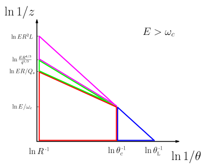
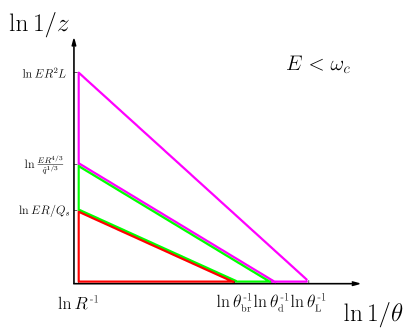
Figure 3: Lund diagram for one vacuum splitting (soft & collinear) where we detail the phase space regimes related to medium scales. All relevant definitions are given in Table​ 1.

We have sketched the Lund diagram for one in-medium splitting in Fig.​ 3 for two possible energy regimes: $E>\omega_{c}$ (left) and $E<\omega_{c}$ (right). The different ordering of the time-scales that were introduced above correspond to the marked areas on the graph and the lines are given by the following set of equations

$$\ell =\ln EL-2y\qquad({t_{\text{f}}}=L)\,,$$ (35)

$$\ell =\ln\frac{E}{\hat{q}^{1/3}}-\frac{4}{3}y\qquad({t_{\text{f}}}=t_{\text{d}})\,,$$ (36)

$$\ell =\ln\frac{E}{Q_{s}}-y\qquad({t_{\text{f}}}=t_{\text{broad}})\,,$$ (37)

where $\ell\equiv\ln 1/z$ and $y\equiv\ln 1/\theta$. In the high-energy case $E>\omega_{c}$, we have also marked the critical angle $\theta_{c}$ with a vertical line. In this case, for $\theta<\theta_{c}$, $t_{\text{broad}}>t_{\text{d}}>L$ and so we have not extended the lines beyond their physical regime.

Scale	Expression
$Q_{s}$	$(\hat{q}L)^{1/2}$
$\omega_{c}$	$\hat{q}L^{2}$
$\theta_{c}$	$(\hat{q}L^{3})^{-1/2}$
$\theta_{\text{d}}$	$(\hat{q}/E^{3})^{1/4}$
$\theta_{\text{broad}}$	$(\hat{q}L)^{1/2}/E$
$\theta_{\text{\tiny L}}$	$(EL)^{-1/2}$

Table 1: Summary of the transverse momentum, energy and angular scales related to medium interactions.

Let us first consider the high-energy regime, i.e. $E>\omega_{c}$, see Fig.​ 3 (left). In order to avoid an interference between the edge of the medium and the non-perturbative scale $Q_{0}$, we also demand for now that $Q_{0}<(RL)^{-1}$. For ease of reference, all the relevant scales are listed in Table​ 1 with a short description. Introducing the quantities $L_{R}\equiv\ln R/\theta_{c}$ and $L_{E}\equiv\ln E/\omega_{c}$, let us describe the various regions below:

(A.1) $\mathbf{{t_{\text{f}}}<t_{\text{broad}}<t_{\text{d}}<L}$ (red region):

Particles are created early in the medium, governed by the quantum mechanical formation time. This corresponds to vacuum-like emissions inside the medium, see also [44, 26]. The phase space is given by

$$(\text{PS})_{1}=L_{R}\left(L_{E}+\frac{1}{2}L_{R}\right)\,,$$ (38)

and is single-logarithmic in the jet energy. The leading term arises for the case when $zE>\omega_{c}$. In fact, all other contributions are sub-leading in the jet energy as long as $t_{\text{d}}<L$, see below, starting from the second term in (38). Furthermore, $t_{\text{d}}<L$ implies that the dipole will decohere in color in a finite distance inside the medium [21, 20], which opens up for the possibility of incoherent energy loss due to secondary medium-induced radiation [44].

(A.2) $\mathbf{t_{\text{broad}}<{t_{\text{f}}}<t_{\text{d}}<L}$ (green region):

In this case, the timescale for broadening is shorter than the quantum mechanical formation time and we expect deviations from pure vacuum-like behavior. This region involves relatively soft splittings, with $zE<\omega_{c}$ and ${\boldsymbol{p}}^{2}<Q_{s}$, and the phase space reads

$$(\text{PS})_{2}=\frac{1}{6}L^{2}_{R}\,,$$ (39)

which is not enhanced by logs of the jet energy.

(A.3) $\mathbf{t_{\text{broad}}<t_{\text{d}}<{t_{\text{f}}}<L}$ (magenta region):

The formation of the dipole in this region is strongly suppressed by the presence of the dipole governing the decoherence of the pair before formation. In particular, this time ordering implies that $\omega/L<{\boldsymbol{p}}^{2}<(\hat{q}zE)^{{\nicefrac{{1}}{{2}}}}$. The phase space is

$$(\text{PS})_{3}=\frac{1}{3}L^{2}_{R}\,,$$ (40)

and is also not enhanced by logs of the jet energy.

(A.4) $\mathbf{{t_{\text{f}}}<L<t_{\text{d}}<t_{\text{broad}}}$ (blue region):

In this case, the splitting takes place inside the medium, but the created partons remain coherent. This happens if the splitting angle is sufficiently small, $\theta<\theta_{c}$ [18, 19]. This implies further that splittings in this region should follow a vacuum emission pattern. The phase space is given by

$$(\text{PS})_{4}=\frac{1}{4}L_{E}^{2}\,,$$ (41)

and is double-logarithmic in the jet energy. In this case the jet is quenched (coherently) due to the presence of a total color charge [46, 44]. It is worth pointing out that this regime does not exist in the low-energy regime, $E<\omega_{c}$. Due to the restriction on the energy, the characteristic decoherence and broadening times are always shorter than the medium length and, in effect, all radiation inside the medium, i.e. ${t_{\text{f}}}<L$, occur at angles $\theta>\theta_{c}$, since $(\omega_{c}\theta^{2})^{-1}<(zE\theta^{2})^{-1}<L$.

(B) $\mathbf{{t_{\text{f}}}>L}$ (beyond the ${t_{\text{f}}}=L$ line):

Splitting takes place outside of the medium, and no medium modification is expected.

To summarize, we have identified two regions of vacuum-like emissions inside the medium, ${t_{\text{f}}}<L$, namely regions A.1 and A.4. However, the fate of the dipole after splitting is expected to be very different. We therefore denote region A.1 as incoherent radiation and region A.4 as coherent radiation.

The total phase space for emissions inside the medium is the sum of the four contributions,

$$(\text{PS})_{{t_{\text{f}}}<L}\,=\,\sum_{i=1}^{4}(\text{PS})_{i}\,=\,\frac{1}{4}\ln^{2}ER^{2}L\,.$$ (42)

Note therefore that there is a relatively large probability of a splitting happening inside the medium, i.e. $(\text{PS})_{{t_{\text{f}}}<L}/(\text{PS})_{\text{tot}}\sim 1/2$ asymptotically when $E\to\infty$. In Monte Carlo simulations, the ratio is slowly varying and lies close to $\sim$40$-$45% [47].

Finally, let us briefly consider the low-energy regime, i.e. $E<\omega_{c}$. In this case, the logarithmic contributions are automatically restricted and the leading-logarithmic approximations should receive significant corrections. However, it is interesting to note that the region ${t_{\text{f}}}<t_{\text{broad}}<t_{\text{d}}$, corresponding to region A.1 in the high-energy regime, scales like

$$(\text{PS})_{{t_{\text{f}}}<t_{\text{broad}},E<\omega_{c}}=\frac{1}{2}\ln^{2}\frac{ER}{Q_{s}}\,.$$ (43)

As pointed out before, the regime of in-medium hard splittings closes whenever $ER\sim Q_{0}$. We will currently not discuss in further detail the remaining phase space regimes, although their impact can be systematically worked out following the steps above.

6 Numerical results

The main result of this work is to demonstrate the factorization property of the medium spectrum given in (26). We have chosen $Q_{0}=0.2$ GeV and $\hat{q}=1.5$ GeV²/fm as reference values, for the high-energy regime we have used $E=1000$ GeV and $L=2$ fm and for the low-energy regime we have chosen $E=240$ GeV and $L=8$ fm. Our final results are presented in Fig.​ 4, where the quantity $F_{\text{med}}$ is defined in Eq. (27). We have plotted the result of evaluating the medium-modification function $F_{\text{med}}$ in the kinematical Lund diagram defined in Fig.​ 3 for both high- and low-energy regimes in Fig.​ 4 (left) and Fig.​ 4 (right) respectively, where the lines in the two figures are equivalent. The full shaded area corresponds to the available phase space given the constraint $k_{\perp}>Q_{0}$, in such a way that the three curves represent (from top to bottom, cf. Fig.​ 3): a) ${t_{\text{f}}}=L$, b) ${t_{\text{f}}}=t_{\text{d}}$ and c) ${t_{\text{f}}}=t_{\text{broad}}$.

It is instructive to examine how the medium modification function behaves for different limits. Commencing our discussion with the high-energy regime, see Fig.​ 4 (left), the regimes where we expect vacuum-like emissions to occur, i.e. at ${t_{\text{f}}}<t_{\text{broad}}<L$ with $t_{\text{d}}>L$ ($\theta<\theta_{c}$) and ${t_{\text{f}}}>L$, the medium modifications are negligible. Indeed, we observe that the onset of modifications follow the line ${t_{\text{f}}}=t_{\text{d}}$ and the main modifications are contained to the regime $t_{\text{broad}}<{t_{\text{f}}}<t_{\text{d}}$, as expected from the discussion in Sec.​ 4. This behavior is more striking, the smaller the coherence angle compared to the cone size. This is of little surprise given that $t_{\text{broad}}$ is related to transverse momentum broadening along the medium length $L$, hence making sense for larger media.

In the low-energy regime, see Fig.​ 4 (right), the same physical picture holds to a large extent. However, the medium modifications are much larger and we also observe a “leakage” into the regime of short formation times. In this case, the scaling behavior we have postulated can only be thought to hold in a parametric sense, and care has to be taken with the assumptions regarding the importance of transverse momentum broadening in order to make any quantitative statements. In Fig.​ 4 (right), the parameters are such that $Q_{0}>(RL)^{-1}$. Apart from serving to prove the expected scaling in the low-energy regime, this parameter choice illustrates that part of the jet, i.e. large-angle and soft emissions, happen to reach the non-perturbative scale while still being “inside” the medium, i.e. their formation times being smaller than $L$. This constitutes a new category of in-medium modifications that goes beyond the scope of our investigation.

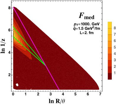
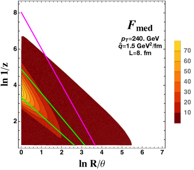
Figure 4: Numerical evaluation of the medium modification factor $F_{\text{med}}$ for in the high-energy ($E>\omega_{c}$, left) and low-energy regime ($E<\omega_{c}$, right) . Notice that the scale of the color coding on the right is rescaled by a factor 10 compared to the left. The shaded area corresponds to the available phase space given the constraint $k_{\perp}>Q_{0}$.

7 Beyond the singlet case

The generalization of the splitting process to arbitrary color representation is straightforward, and does not modify the general structure of Eq. (26). One simply has to replace the coupling constant $\alpha_{\text{em}}\to\alpha_{s}$ and the Altarelli-Parisi splitting function for the relevant one, e.g. $P_{q\gamma}(z)\to P_{ij}(z)$ in the vacuum spectrum (23). In the medium modification factor $F_{\text{med}}$ one has to account for the more involved color algebra. Taken as a concrete example the splitting process $q\to q+g$, we would replace the expressions for the dipole and quadrupole by,

$$S_{12}(\bar{t},t) \to\frac{1}{N_{c}^{2}-1}\left\langle{\rm tr}\left(V_{2}^{\dagger}(t,\bar{t})V_{1}(\bar{t},t)\right){\rm tr}\left(V_{0}^{\dagger}(t,\bar{t})V_{2}(\bar{t},t)\right)-\frac{1}{N_{c}}{\rm tr}\left(V_{0}^{\dagger}(t,\bar{t})V_{1}(\bar{t},t)\right)\right\rangle\,,$$ (44)

$$Q \to\frac{1}{N_{c}^{2}-1}\left\langle{\rm tr}\left(V_{\bar{1}}^{\dagger}(\bar{t},L)V_{1}(L,\bar{t})V_{2}^{\dagger}(\bar{t},L)V_{\bar{2}}(L,\bar{t})\right){\rm tr}\left(V_{\bar{2}}^{\dagger}(\bar{t},L)V_{2}(L,\bar{t})\right)\right.$$

$$\qquad\quad\left.-\frac{1}{N_{c}}{\rm tr}\left(V_{\bar{1}}^{\dagger}(\bar{t},L)V_{1}(L,\bar{t})\right)\right\rangle\,.$$ (45)

In the large $N_{c}$ limit, the second term in both expressions above can be neglected, in which case we are left with the replacement

$$S_{12}(\bar{t},t) \to S_{12}(\bar{t},t)S_{20}(\bar{t},t)\,,$$ (46)

$$Q \to Q(L,\bar{t})S_{2\bar{2}}(L,\bar{t})\,.$$ (47)

The appearance of these new dipole structures, $S_{20}(\bar{t},t)$ and $S_{2\bar{2}}(L,\bar{t})$, does not render it impossible to transfer the qualitative insight regarding color-singlet dipole splittings to color-charged ones. In the harmonic oscillator approximation, we find that

$$S_{20}(\bar{t},t) ={\rm e}^{-\frac{1}{12}\hat{q}(1-z)^{2}\theta^{2}\tau^{3}},$$ (48)

$$S_{2\bar{2}}(L,\bar{t},t) ={\rm e}^{-\frac{1}{4}\hat{q}z^{2}\theta^{2}(L-t^{\prime})\tau^{2}},$$ (49)

where we have defined ${\boldsymbol{r}}_{20}(s)={\boldsymbol{n}}_{1}(s-t)$ and ${\boldsymbol{r}}_{2\bar{2}}(s)={\boldsymbol{n}}_{2}(t^{\prime}-t)$.

Focussing for the moment on the dynamics during formation, we note that the combination $S_{12}S_{20}$ only depends on the jet quenching parameter through the combination $\hat{q}_{\text{eff}}=\hat{q}(1+(1-z)^{2})\approx((1-z)N_{c}+z^{2}C_{F})\hat{\bar{q}}$ in the large-$N_{c}$ limit (recall that, in our calculation so far, $\hat{q}=C_{F}\hat{\bar{q}}$). This effective $\hat{q}_{\text{eff}}$ was indeed previously identified for medium-induced quark-gluon splitting, see e.g. [40].

Similar conclusions can be drawn regarding the correction to the quadrupole. Therefore, although our general discussion was based on the calculation of a color-singlet splitting, we see that it can be straightforwardly generalized to splittings involving a non-zero total color charge by carefully considering the color dependence of $\hat{q}_{\text{eff}}$, as well as the expected replacements in the vacuum spectrum. This validates our discussion of soft and collinear radiation in terms of the Lund plane introduced in Sec.​ 5.

8 Conclusions and outlook

We have studied the production of hard radiation in the presence of a quark-gluon plasma, and have found two regimes of vacuum-like emissions inside the medium. By vacuum-like, we simply mean that the in-medium splitting function is equal to the one in the vacuum, or $F_{\text{med}}\approx 0$. These cases include a) the regime of short formation time, in particular ${t_{\text{f}}}<t_{\text{broad}}<L$ (corresponding to the region A.1 in Fig.​ 3), and at small angles, concretely $\theta<\theta_{c}$ (corresponding to region A.4 in Fig.​ 3). The fate of these two types of emissions is however different since only in the former regime do the splitting products lose their color coherence at a finite distance inside the medium. Due to this rapid decoherence, the splitting products should therefore become subject to independent energy loss processes. In contrast, emissions in region A.4 are color coherent when they exit the medium and should therefore lose energy as a whole.

We have also identified the border at which long-distance medium effects start to play a role in the splitting process. In particular at ${t_{\text{f}}}\gtrsim t_{\text{broad}}$, where the relative transverse momentum ${\boldsymbol{p}}^{2}<Q_{s}^{2}$, the opening angle of the jet could vary significantly due to transverse momentum broadening. These features are also recovered in our numerical calculations in Sec.​ 6. Hence, this study confirms the notion of purely vacuum-like emissions that are emitted inside the medium.

The spectrum of these excitations follow from a “semi-classical” picture, where the original splitting takes place immediately after the hard process. Our analysis of time-scales further corroborates the validity of our assumptions for the regions of vacuum-like emissions. A further, quantitative study of the regions where ${t_{\text{f}}}$ is similar to $t_{\text{broad}}$ and $t_{\text{d}}$ demands that we include the possibility of transverse momentum broadening, i.e. relax the assumption of straight-line trajectories, for further details see [39, 40].

Computing higher-order splitting processes, and their virtual corrections, goes beyond the scope of this paper, and will be pursued in the future. We already anticipate that our analysis points to mismatch between real and virtual terms, since the latter do not involve the long-time component of the processes encoded, in our case, in the quadrupole. Such a mismatch, albeit due to energy loss processes, was already shown to entail novel resummation schemes to account for medium modifications on multi-parton probes, such as jets [25].

Appendix A Beyond the classical picture

Applying the limit $E\to\infty$ and using the previously derived dressed propagator in Eq. (10), we obtain the amplitude,

$$\mathcal{M}^{\rm in}_{\gamma\rightarrow q\bar{q}} =\frac{e}{E}\gamma^{\gamma\to q\bar{q}}_{\lambda,s,s^{\prime}}(z)\,\int_{0}^{L}{\rm d}t\,{\rm e}^{-i(L-t)/{t_{\text{f}}}}$$

$$\times\Big{[}{\boldsymbol{p}}+i[(1-z)\boldsymbol{\partial}_{x_{1}}-z\boldsymbol{\partial}_{x_{2}}]\Big{]}\cdot{\boldsymbol{\epsilon}}_{\lambda}[V_{1}(t_{L},t)V^{\dagger}_{2}(t_{L},t)]_{ij}\big{|}_{{\boldsymbol{x}}_{1}={\boldsymbol{x}}_{2}={\boldsymbol{n}}_{0}t}\,,$$ (50)

up to factors that cancel out in the cross section, and where ${\boldsymbol{n}}_{0}=({\boldsymbol{p}}_{1}+{\boldsymbol{p}}_{2})/E$. Note that, in this case, the trajectories of the dipole constituents are described by ${\boldsymbol{r}}_{i}\equiv{\boldsymbol{x}}_{i}+(s-t){\boldsymbol{n}}_{i}$, while in Sec.​ 2 we assumed that ${\boldsymbol{x}}_{i}=0$.

The “in-in” and “in-out” emission spectra then become

$$\frac{{\rm d}N^{\text{in-in}}}{{\rm d}z\,{\rm d}{\boldsymbol{p}}^{2}} =\frac{{\rm d}N^{\text{vac}}}{{\rm d}z\,{\rm d}{\boldsymbol{p}}^{2}}\;2{\rm Re}\int_{0}^{L}\frac{{\rm d}t}{{t_{\text{f}}}}\int_{t}^{L}\frac{{\rm d}\bar{t}}{{t_{\text{f}}}}\,{\rm e}^{-i\frac{\bar{t}-t}{{t_{\text{f}}}}}\,\mathcal{\hat{V}}_{1}\big{[}Q(L,\bar{t})S_{12}(\bar{t},t)\big{]}_{\begin{subarray}{c}{\boldsymbol{x}}_{2}={\boldsymbol{x}}_{1}={\boldsymbol{n}}_{0}t\\ \bar{\boldsymbol{x}}_{2}=\bar{\boldsymbol{x}}_{1}={\boldsymbol{n}}_{0}\bar{t}\end{subarray}}\,,$$ (51)

and

$$\frac{{\rm d}N^{\text{in-out}}}{{\rm d}z\,{\rm d}{\boldsymbol{p}}^{2}}=\frac{{\rm d}N^{\text{vac}}}{{\rm d}z\,{\rm d}{\boldsymbol{p}}^{2}}\;2\text{Im}\int_{0}^{L}\frac{{\rm d}t}{{t_{\text{f}}}}\,{\rm e}^{-i\frac{L-t}{{t_{\text{f}}}}}\mathcal{\hat{V}}_{2}\big{[}S_{12}(L,t)\big{]}_{{\boldsymbol{x}}_{2}={\boldsymbol{x}}_{1}={\boldsymbol{n}}_{0}t}\,,$$ (52)

where ${t_{\text{f}}}=2z(1-z)E/{\boldsymbol{p}}^{2}$ and we have introduced the operators

$$\mathcal{\hat{V}}_{1} =\frac{1}{{\boldsymbol{p}}^{2}}\Big{(}{\boldsymbol{p}}+i[(1-z)\boldsymbol{\partial}_{x_{1}}-z\boldsymbol{\partial}_{x_{2}}]\Big{)}\cdot\Big{(}{\boldsymbol{p}}-i[(1-z)\boldsymbol{\partial}_{\bar{x}_{1}}-z\boldsymbol{\partial}_{\bar{x}_{2}}]\Big{)}\,,$$ (53)

$$\mathcal{\hat{V}}_{2} =\frac{{\boldsymbol{p}}}{{\boldsymbol{p}}^{2}}\cdot\big{(}{\boldsymbol{p}}+i[(1-z)\boldsymbol{\partial}_{x_{1}}-z\boldsymbol{\partial}_{x_{2}}]\big{)}\,.$$ (54)

The dipole term, comprising the additional shift of the initial positions of the Wilson lines, reads

$$S_{12}(t_{1},t_{0})=\exp\left\{-\frac{1}{4}\hat{q}\Delta t\left[\left({\boldsymbol{x}}_{12}+\frac{1}{2}\Delta t{\boldsymbol{n}}_{12}\right)^{2}+\frac{1}{12}\Delta t^{2}{\boldsymbol{n}}_{12}^{2}\right]\right\}\,,$$ (55)

for generic time intervals, where $\Delta t=t_{1}-t_{0}$ and ${\boldsymbol{x}}_{12}\equiv{\boldsymbol{x}}_{1}-{\boldsymbol{x}}_{2}$, while the missing terms in the quadrupole (18) read, explicitly $S_{I\bar{I}}(t_{1},t_{0})=\exp[-\frac{1}{4}\hat{q}\Delta t\,({\boldsymbol{x}}_{I\bar{I}}+{\boldsymbol{n}}_{I}\tau)^{2}]$, using the definition in (17).

Because of the constraints on the initial transverse position in the amplitude and the complex conjugate, leading respectively to ${\boldsymbol{x}}_{1}={\boldsymbol{x}}_{2}$ and $\bar{\boldsymbol{x}}_{1}=\bar{\boldsymbol{x}}_{2}$, the resulting spectra will be similar to the terms derived to obtain Eq. (26), with the definition in (27), except for a unique pre-factor appearing under the integrals of the “in-in” and the “in-out” terms that arises from the more involved vertices in (51) and (52).

We have analyzed these terms in detail for the factorizable piece of the “in-in” term and for the “in-out” term. In particular, for the “in-in” term the correction factor appearing under the integral reads

$$1-i\frac{\hat{q}\tau^{2}}{4z(1-z)E}-i\frac{\hat{q}\tau_{L}\tau\xi}{z(1-z)E}-\left(\frac{\hat{q}\tau_{L}\tau\xi}{2z(1-z)E}\right)^{2}\left(1+\frac{\tau}{2\xi\tau_{L}}\right)+\frac{\hat{q}\tau_{L}\xi}{(z(1-z)E\theta)^{2}}\,,$$ (56)

where we defined $\tau_{L}\equiv L-\bar{t}$ and $\xi\equiv(1-z)^{2}+z^{2}$ to shorten the expression. For the in-out term the correction factor is $1-i\hat{q}(L-t)^{2}/[4z(1-z)E]$, which closely resembles the two first terms in (56) with $\tau$ substituted by $L-t$. Neglecting all finite-$z$ corrections and assuming short times, $L\gg t,\bar{t}$, these terms scale as

$$1-i\frac{{t_{\text{f}}}}{t_{\text{d}}}\left(\frac{\tau}{t_{\text{d}}}\right)^{2}-i\frac{{t_{\text{f}}}}{t_{\text{broad}}}\frac{\tau}{t_{\text{broad}}}-\left(\frac{{t_{\text{f}}}}{t_{\text{broad}}}\right)^{2}\left(\frac{\tau}{t_{\text{broad}}}\right)^{2}+\left(\frac{{t_{\text{f}}}}{t_{\text{broad}}}\right)^{2}\,.$$ (57)

This clearly demonstrates that the corrections to the vertex start to play a role whenever the (kinematical) formation time ceases to constitute the shortest time-scale to which compare the difference of emission times $\tau$. In particular, this starts to happen then $\tau\lesssim t_{\text{broad}}<{t_{\text{f}}}$.

References

- [1] D. d’Enterria, Jet quenching, Landolt-Bornstein 23 (2010) 471. arXiv:0902.2011.
- [2] A. Majumder, M. Van Leeuwen, The Theory and Phenomenology of Perturbative QCD Based Jet Quenching, Prog.Part.Nucl.Phys. A66 (2011) 41–92. arXiv:1002.2206.
- [3] Y. Mehtar-Tani, J. G. Milhano, K. Tywoniuk, Jet physics in heavy-ion collisions, Int. J. Mod. Phys. A28 (2013) 1340013. arXiv:1302.2579.
- [4] J. Adams, et al., Experimental and theoretical challenges in the search for the quark gluon plasma: The STAR Collaboration’s critical assessment of the evidence from RHIC collisions, Nucl.Phys. A757 (2005) 102–183.
- [5] K. Adcox, et al., Formation of dense partonic matter in relativistic nucleus-nucleus collisions at RHIC: Experimental evaluation by the PHENIX collaboration, Nucl.Phys. A757 (2005) 184–283.
- [6] K. Aamodt, et al., Suppression of Charged Particle Production at Large Transverse Momentum in Central Pb-Pb Collisions at 2.76 TeV, Phys. Lett. B696 (2011) 30–39. arXiv:1012.1004.
- [7] V. Khachatryan, et al., Charged-particle nuclear modification factors in PbPb and pPb collisions at TeV, JHEP 04 (2017) 039. arXiv:1611.01664.
- [8] S. Chatrchyan, et al., Observation and studies of jet quenching in PbPb collisions at nucleon-nucleon center-of-mass energy = 2.76 TeV, Phys.Rev. C84 (2011) 024906. arXiv:1102.1957.
- [9] G. Aad, et al., Observation of a Centrality-Dependent Dijet Asymmetry in Lead-Lead Collisions at TeV with the ATLAS Detector at the LHC, Phys. Rev. Lett. 105 (2010) 252303. arXiv:1011.6182.
- [10] B. Abelev, et al., Measurement of charged jet suppression in Pb-Pb collisions at = 2.76 TeV, JHEP 03 (2014) 013. arXiv:1311.0633.
- [11] S. Acharya, et al., First measurement of jet mass in PbPb and pPb collisions at the LHC, Phys. Lett. B776 (2018) 249–264. arXiv:1702.00804.
- [12] A. M. Sirunyan, et al., Measurement of the groomed jet mass in PbPb and pp collisions at TeV, JHEP 10 (2018) 161. arXiv:1805.05145.
- [13] F. D’Eramo, M. Lekaveckas, H. Liu, K. Rajagopal, Momentum Broadening in Weakly Coupled Quark-Gluon Plasma (with a view to finding the quasiparticles within liquid quark-gluon plasma), JHEP 05 (2013) 031. arXiv:1211.1922.
- [14] L. Apolinrio, J. G. Milhano, G. P. Salam, C. A. Salgado, Probing the time structure of the quark-gluon plasma with top quarks, Phys. Rev. Lett. 120 (23) (2018) 232301. arXiv:1711.03105.
- [15] C. Andres, N. Armesto, H. Niemi, R. Paatelainen, C. A. Salgado, Jet quenching as a probe of the initial stages in heavy-ion collisionsarXiv:1902.03231.
- [16] H. A. Andrews, et al., Novel tools and observables for jet physics in heavy-ion collisionsarXiv:1808.03689.
- [17] Y. Mehtar-Tani, Relating the description of gluon production in pA collisions and parton energy loss in AA collisions, Phys. Rev. C75 (2007) 034908. arXiv:hep-ph/0606236.
- [18] Y. Mehtar-Tani, C. A. Salgado, K. Tywoniuk, Anti-angular ordering of gluon radiation in QCD media, Phys. Rev. Lett. 106 (2011) 122002. arXiv:1009.2965.
- [19] Y. Mehtar-Tani, C. A. Salgado, K. Tywoniuk, Jets in QCD Media: From Color Coherence to Decoherence, Phys. Lett. B707 (2012) 156–159. arXiv:1102.4317.
- [20] Y. Mehtar-Tani, C. A. Salgado, K. Tywoniuk, The Radiation pattern of a QCD antenna in a dense medium, JHEP 10 (2012) 197. arXiv:1205.5739.
- [21] J. Casalderrey-Solana, E. Iancu, Interference effects in medium-induced gluon radiation, JHEP 08 (2011) 015. arXiv:1105.1760.
- [22] J. Casalderrey-Solana, D. Pablos, K. Tywoniuk, Two-gluon emission and interference in a thin QCD medium: insights into jet formation, JHEP 11 (2016) 174. arXiv:1512.07561.
- [23] J. G. Milhano, K. C. Zapp, Origins of the di-jet asymmetry in heavy ion collisions, Eur. Phys. J. C76 (5) (2016) 288. arXiv:1512.08107.
- [24] J. Casalderrey-Solana, D. Gulhan, G. Milhano, D. Pablos, K. Rajagopal, Angular Structure of Jet Quenching Within a Hybrid Strong/Weak Coupling Model, JHEP 03 (2017) 135. arXiv:1609.05842.
- [25] Y. Mehtar-Tani, K. Tywoniuk, Sudakov suppression of jets in QCD media, Phys. Rev. D98 (5) (2018) 051501. arXiv:1707.07361.
- [26] P. Caucal, E. Iancu, A. H. Mueller, G. Soyez, Vacuum-like jet fragmentation in a dense QCD medium, Phys. Rev. Lett. 120 (2018) 232001. arXiv:1801.09703.
- [27] B. Andersson, G. Gustafson, L. Lönnblad, U. Pettersson, Coherence Effects in Deep Inelastic Scattering, Z. Phys. C43 (1989) 625.
- [28] Y.-T. Chien, R. Kunnawalkam Elayavalli, Probing heavy ion collisions using quark and gluon jet substructurearXiv:1803.03589.
- [29] F. A. Dreyer, G. P. Salam, G. Soyez, The Lund Jet Plane, JHEP 12 (2018) 064. arXiv:1807.04758.
- [30] L. Cunqueiro, M. Posko, Searching for the dead cone effects with iterative declustering of heavy-flavor jets, Phys. Rev. D99 (7) (2019) 074027. arXiv:1812.00102.
- [31] S. Marzani, G. Soyez, M. Spannowsky, Looking inside jets: an introduction to jet substructure and boosted-object phenomenology[Lect. Notes Phys.958,pp.(2019)]. arXiv:1901.10342.
- [32] U. A. Wiedemann, Transverse dynamics of hard partons in nuclear media and the QCD dipole, Nucl. Phys. B582 (2000) 409–450. arXiv:hep-ph/0003021.
- [33] U. A. Wiedemann, Gluon radiation off hard quarks in a nuclear environment: Opacity expansion, Nucl. Phys. B588 (2000) 303–344. arXiv:hep-ph/0005129.
- [34] R. Baier, Y. L. Dokshitzer, A. H. Mueller, S. Peigne, D. Schiff, Radiative energy loss of high-energy quarks and gluons in a finite volume quark - gluon plasma, Nucl.Phys. B483 (1997) 291–320. arXiv:hep-ph/9607355.
- [35] B. Zakharov, Radiative energy loss of high-energy quarks in finite size nuclear matter and quark - gluon plasma, JETP Lett. 65 (1997) 615–620. arXiv:hep-ph/9704255.
- [36] M. Gyulassy, P. Levai, I. Vitev, Reaction operator approach to nonAbelian energy loss, Nucl.Phys. B594 (2001) 371–419. arXiv:nucl-th/0006010.
- [37] X.-N. Wang, X.-f. Guo, Multiple parton scattering in nuclei: Parton energy loss, Nucl.Phys. A696 (2001) 788–832. arXiv:hep-ph/0102230.
- [38] P. B. Arnold, G. D. Moore, L. G. Yaffe, Photon and gluon emission in relativistic plasmas, JHEP 0206 (2002) 030. arXiv:hep-ph/0204343.
- [39] J.-P. Blaizot, F. Dominguez, E. Iancu, Y. Mehtar-Tani, Medium-induced gluon branching, JHEP 01 (2013) 143. arXiv:1209.4585.
- [40] L. Apolinário, N. Armesto, J. G. Milhano, C. A. Salgado, Medium-induced gluon radiation and colour decoherence beyond the soft approximation, JHEP 02 (2015) 119. arXiv:1407.0599.
- [41] M. D. Sievert, I. Vitev, B. Yoon, A complete set of in-medium splitting functions to any order in opacityarXiv:1903.06170.
- [42] T. Altinoluk, N. Armesto, G. Beuf, M. Martnez, C. A. Salgado, Next-to-eikonal corrections in the CGC: gluon production and spin asymmetries in pA collisions, JHEP 07 (2014) 068. arXiv:1404.2219.
- [43] T. Altinoluk, N. Armesto, G. Beuf, A. Moscoso, Next-to-next-to-eikonal corrections in the CGC, JHEP 01 (2016) 114. arXiv:1505.01400.
- [44] Y. Mehtar-Tani, K. Tywoniuk, Radiative energy loss of neighboring subjets, Nucl. Phys. A979 (2018) 165–203. arXiv:1706.06047.
- [45] J. Casalderrey-Solana, C. A. Salgado, Introductory lectures on jet quenching in heavy ion collisions, Acta Phys. Polon. B38 (2007) 3731–3794. arXiv:0712.3443.
- [46] J. Casalderrey-Solana, Y. Mehtar-Tani, C. A. Salgado, K. Tywoniuk, New picture of jet quenching dictated by color coherence, Phys. Lett. B725 (2013) 357–360. arXiv:1210.7765.
- [47] J. Casalderrey-Solana, J. G. Milhano, P. Quiroga-Arias, Out of Medium Fragmentation from Long-Lived Jet Showers, Phys. Lett. B710 (2012) 175–181. arXiv:1111.0310.