Analytical model for gravitational-wave echoes from spinning remnants

Abstract

Gravitational-wave echoes in the post-merger signal of a binary coalescence are predicted in various scenarios, including near-horizon quantum structures, exotic states of matter in ultracompact stars, and certain deviations from general relativity. The amplitude and frequency of each echo is modulated by the photon-sphere barrier of the remnant, which acts as a spin- and frequency-dependent high-pass filter, decreasing the frequency content of each subsequent echo. Furthermore, a major fraction of the energy of the echo signal is contained in low-frequency resonances corresponding to the quasi-normal modes of the remnant. Motivated by these features, in this work we provide an analytical gravitational-wave template in the low-frequency approximation describing the post-merger ringdown and the echo signal of a spinning ultracompact object. Besides the standard ringdown parameters, the template is parametrized in terms of only two physical quantities: the reflectivity coefficient and the compactness of the remnant. We discuss novel effects related to the spin and to the complex reflectivity, such as a more involved modulation of subsequent echoes, the mixing of two polarizations, and the ergoregion instability in case of perfectly-reflecting spinning remnants. Finally, we compute the errors in the estimation of the template parameters with current and future gravitational-wave detectors using a Fisher matrix framework. Our analysis suggests that models with almost perfect reflectivity can be excluded/detected with current instruments, whereas probing values of the reflectivity smaller than $80\%$ at $3\sigma$ confidence level requires future detectors (Einstein Telescope, Cosmic Explorer, LISA). The template developed in this work can be easily implemented to perform a matched-filter based search for echoes and to constrain models of exotic compact objects.

I Introduction

Gravitational-wave (GW) echoes in the post-merger signal of a compact binary coalescence might be a smoking gun of near-horizon quantum structures Cardoso:2016rao ; Cardoso:2016oxy ; Oshita:2018fqu ; Wang:2019rcf , exotic compact objects (ECOs), exotic states of matter in ultracompact stars Ferrari:2000sr ; Pani:2018flj ; Buoninfante:2019swn , and of modified theories of gravity Buoninfante:2019teo ; Delhom:2019btt (see Cardoso:2017cqb ; Cardoso:2017njb ; LRR for some recent reviews). Detecting echoes in the GW data of LIGO/Virgo and of future GW observatories would allow us to probe the near-horizon structure of compact objects. The absence of echoes in GW data could instead place increasingly stronger constraints on alternatives to the black-hole (BH) paradigm.

Tentative evidence for echoes in the combined LIGO/Virgo binary BH events Abedi:2016hgu ; Conklin:2017lwb and in the neutron-star binary coalescence GW170817 Abedi:2018npz have been reported, followed by controversial claims about the statistical significance of such results Abedi:2016hgu ; Ashton:2016xff ; Abedi:2017isz ; Conklin:2017lwb ; Westerweck:2017hus ; Abedi:2018pst , and by recent negative searches using a more accurate template UchikataEchoes and a morphology-independent algorithm Tsang2019 . Performing a reliable search for echoes requires developing data analysis techniques as well as constructing accurate waveform models. Here we focus on the latter challenge.

While several features of the signal have been understood theoretically LRR , an important open problem is to develop templates for echoes that are both accurate and practical for searches in current and future detectors, which might complement model-independent Abedi:2018npz ; Conklin:2017lwb ; Conklin:2019fcs and burst Tsang:2018uie ; Lin:2019qyx ; Tsang2019 searches, the latter being independent of the morphology of the echo waveform. Furthermore, using an accurate template is crucial for model selection and to discriminate the origin of the echoes in case of a detection. There has been a considerable progress in modeling the echo waveform Nakano:2017fvh ; Mark:2017dnq ; Maselli:2017tfq ; Bueno:2017hyj ; Wang:2018mlp ; Correia:2018apm ; Wang:2018gin ; UchikataEchoes , but the approaches adopted so far are not optimal, since they are either based on analytical templates not necessarily related to the physical properties of the remnant, or rely on model-dependent numerical waveforms which are inconvenient for matched filtered searches and can be computationally expensive. In this paper, we provide an analytical, physically motivated template that is parametrized by the standard ringdown parameters plus two physical quantities related to the properties of the exotic remnant. Our template can be easily implemented in a matched filter based data analysis.

We extend the recent analytical template of Ref. Testa:2018bzd to include spin effects. This is particularly important for various reasons. First, merger remnants are typically rapidly spinning (dimensionless spin $\chi\approx 0.7$ in case of nonspinning binaries, due to angular-momentum conservation); second, the spin might introduce nontrivial effects in the shape and modulation of echoes; finally, spinning ECOs have a rich phenomenology LRR , for example they might undergo various types of instabilities 1978CMaPh..63..243F ; Moschidis:2016zjy ; Brito:2015oca ; Cardoso:2007az ; Cardoso:2008kj ; Chirenti:2008pf ; Cardoso:2014sna ; Maggio:2017ivp ; Maggio:2018ivz . In particular, if an ergoregion instability Cardoso:2014sna ; Vicente:2018mxl ; Brito:2015oca occurs, the signal would grow exponentially in time over a time scale which is generically parametrically longer than the time delay between echoes, and it is always much longer than the object’s dynamical time scale Barausse:2018vdb .

In this work we use $G=c=1$ units.

II Analytical echo template

Reference Mark:2017dnq presents a framework for modeling the echoes from nonspinning ECOs by reprocessing the standard BH ringdown (at the horizon) using a transfer function ${\cal K}$, which encodes the information about the physical properties of the remnant, such as its reflectivity. Our approach is based on this framework, but we extended its scope to gravitational perturbations of spinning ECOs. Our goal is to model the echo signal analytically, following a prescription similar to that of the nonspinning case studied in Ref. Testa:2018bzd . The key difference between the present work and Ref. Testa:2018bzd is that in the latter the effective potential for the perturbations of the Schwarzschild geometry was approximated using a Pöschl-Teller potential Poschl:1933zz ; Ferrari:1984zz in order to obtain an analytical solution for BH perturbations. In this work, we use a low-frequency approximation to solve Teukolsky’s equation analytically. We get an analytical transfer function (see Eq. (18) below) by approximating the BH reflection (${\cal R}_{\rm BH}$) and transmission (${\cal T}_{\rm BH}$) coefficients. Our final template is provided in a ready-to-be-used form in a supplemental Mathematica^® notebook webpage .

II.1 Background

We consider a spinning compact object with radius $r_{0}$, whose exterior geometry ($r>r_{0}$) is described by the Kerr metric Maggio:2017ivp ; Abedi:2016hgu ; Wang:2018gin ; Barausse:2018vdb . Unlike the case of spherically symmetric spacetimes, the absence of Birkhoff’s theorem in axisymmetry does not ensure that the vacuum region outside a spinning object is described by the Kerr geometry. This implies that the multipolar structure of a spinning ECO might be different from that of a Kerr BH Raposo:2018xkf ; Barcelo:2019aif . Nevertheless, for perturbative solutions to the vacuum Einstein’s equation that admit a smooth BH limit, all multipole moments of the external spacetime approach those of a Kerr BH in the high-compactness regime Raposo:2018xkf (for specific examples, see Pani:2015tga ; Uchikata:2015yma ; Uchikata:2016qku ; Yagi:2015hda ; Yagi:2015upa ; Posada-Aguirre:2016qpz ).

Therefore, in Boyer-Lindquist coordinates, the line element at $r>r_{0}$ reads

$$ds^{2} =-\left(1-\frac{2Mr}{\Sigma}\right)dt^{2}+\frac{\Sigma}{\Delta}dr^{2}-\frac{4Mr}{\Sigma}a\sin^{2}\theta d\phi dt$$ (1)

$$+ {\Sigma}d\theta^{2}+\left[(r^{2}+a^{2})\sin^{2}\theta+\frac{2Mr}{\Sigma}a^{2}\sin^{4}\theta\right]d\phi^{2}\,,$$

In the above equation $\Sigma=r^{2}+a^{2}\cos^{2}\theta$ and $\Delta=r^{2}+a^{2}-2Mr=(r-r_{+})(r-r_{-})$, where $r_{\pm}=M\pm\sqrt{M^{2}-a^{2}}$; $M$ and $J\equiv aM\equiv\chi M^{2}$ are the total mass and angular momentum of the object respectively.

The properties of the object’s interior and surface can be parametrized in terms of boundary conditions at $r=r_{0}$, in particular by a complex and (possibly) frequency-and-spin-dependent reflection coefficient, ${\cal R}$ Mark:2017dnq ; Maggio:2017ivp . Motivated by models of microscopic corrections at the horizon scale, in the following we focus on the case

$$r_{0}=r_{+}(1+\epsilon)\qquad 0<\epsilon\ll 1\,,$$ (2)

where $r_{+}$ is the location of the would-be horizon. We fix $r_{0}$ (or, equivalently, $\epsilon$), by requiring the location of the surface to be at a proper length $\delta\ll M$ from $r_{+}$, where

$$\delta=\int_{r_{+}}^{r_{0}}dr\,\sqrt{g_{rr}}|_{\theta=0}\,.$$ (3)

This implies

$$\epsilon\simeq\sqrt{1-\chi^{2}}\frac{\delta^{2}}{4r_{+}^{2}}\,,$$ (4)

in the $\delta/M\ll 1$ limit.

We shall use $M$, $\chi$, and $\delta/M$ to parametrize the background geometry, and ${\cal R}$ to model the boundary conditions for perturbations.

II.2 Linear perturbations

Scalar, electromagnetic and gravitational perturbations in the exterior Kerr geometry are described by Teukolsky’s master equations Teukolsky:1972my ; Teukolsky:1973ha ; Teukolsky:1974yv , the radial solution of which shall be denoted by ${}_{s}R_{lm}(r,\omega)$ (see Appendix A).

It is convenient to make a change of variables by introducing the Detweiler’s function 1977RSPSA.352..381D ; Maggio:2018ivz

$$\tilde{\Psi}=\Delta^{s/2}\sqrt{r^{2}+a^{2}}\left[\alpha\ _{s}R_{lm}+\beta\Delta^{s+1}\frac{d_{s}R_{lm}}{dr}\right]\,,$$ (5)

where $\alpha$ and $\beta$ are certain radial functions 1977RSPSA.352..381D ; Maggio:2018ivz that satisfy the following relation

$$\alpha^{2}-\alpha^{\prime}\beta\Delta^{s+1}+\alpha\beta^{\prime}\Delta^{s+1}-\beta^{2}\Delta^{2s+1}V_{S}=\text{constant}\,.$$ (6)

The radial potential $V_{S}$ is defined below in Eq. (12), and $s=0,\pm 1,\pm 2$ for scalar, electromagnetic and gravitational perturbations, respectively. By introducing the tortoise coordinate $x$, defined as

$$\frac{dx}{dr}=\frac{r^{2}+a^{2}}{\Delta}\,,$$ (7)

Teukolsky’s master equation becomes

$$\frac{d^{2}\tilde{\Psi}}{dx^{2}}-V(r,\omega)\tilde{\Psi}=\tilde{S}\,.$$ (8)

Here $\tilde{S}$ is a source term and the effective potential reads as

$$V(r,\omega)=\frac{U\Delta}{(r^{2}+a^{2})^{2}}+G^{2}+\frac{dG}{dx}\,,$$ (9)

with

$$G = \frac{s(r-M)}{r^{2}+a^{2}}+\frac{r\Delta}{(r^{2}+a^{2})^{2}}\,,$$ (10)

$$U = V_{S}+\frac{2\alpha^{\prime}+(\beta^{\prime}\Delta^{s+1})^{\prime}}{\beta\Delta^{s}}\,,$$ (11)

$$V_{S} = -\frac{1}{\Delta}\left[K^{2}-is\Delta^{\prime}K+\Delta(2isK^{\prime}-\lambda_{s})\right]\,,$$ (12)

and $K=(r^{2}+a^{2})\omega-am$. The prime denotes a derivative with respect to $r$. Remarkably, the functions $\alpha$ and $\beta$ can be chosen such that the resulting potential (9) is purely real 1977RSPSA.352..381D ; Maggio:2018ivz . Although the choice of $\alpha$ and $\beta$ is not unique, $\tilde{\Psi}$ evaluated at the asymptotic infinities ($x\to\pm\infty$) remains unchanged up to a phase. Therefore, the energy and angular momentum fluxes are not affected Chandra .

The asymptotic behavior of the potential is

$$V\to\left\{\begin{array}[]{ll}-\omega^{2}&\quad{\rm as}\,\,x\to+\infty\\ -k^{2}&\quad{\rm as}\,\,x\to-\infty\end{array}\right.\,,$$ (13)

where $k=\omega-m\Omega$ and $\Omega=a/(2Mr_{+})$ is the angular velocity at the event horizon of a Kerr BH.

II.3 Transfer function

Equation (8) is formally equivalent to the static scalar case Mark:2017dnq and can be solved using Green’s function techniques. At asymptotic infinity, we require the solution of Eq. (8) to be an outgoing wave, $\tilde{\Psi}(\omega,x\to\infty)\sim\tilde{Z}^{+}(\omega)e^{i\omega x}$. Similarly to what shown in Ref. Mark:2017dnq we have

$$\tilde{Z}^{+}(\omega)=\tilde{Z}_{\rm BH}^{+}(\omega)+{\cal K}(\omega)\tilde{Z}_{\rm BH}^{-}(\omega)\,.$$ (14)

In the above equation, $\tilde{Z}_{\rm BH}^{\pm}$ are the responses of a Kerr BH (at infinity and near the horizon, for the plus and minus signs, respectively) to the source $\tilde{S}$, i.e.

$$\tilde{Z}_{\rm BH}^{\pm}(\omega)=\frac{1}{W_{\rm BH}}\int_{-\infty}^{+\infty}dx{\tilde{S}\tilde{\Psi}_{\mp}}\,,$$ (15)

where $\tilde{\Psi}_{\pm}$ are two independent solutions of the homogeneous equation associated to Eq. (8) such that

$$\tilde{\Psi}_{+}(\omega,x)\sim\begin{cases}\displaystyle e^{+i\omega x}&\text{ as }x\to+\infty\\ \displaystyle B_{\rm out}(\omega)e^{+ikx}+B_{\rm in}(\omega)e^{-ikx}&\text{ as }x\to-\infty\end{cases}\,,\\$$ (16)

$$\tilde{\Psi}_{-}(\omega,x)\sim\begin{cases}\displaystyle A_{\rm out}(\omega)e^{+i\omega x}+A_{\rm in}(\omega)e^{-i\omega x}&\text{ as }x\to+\infty\\ \displaystyle e^{-ikx}&\text{ as }x\to-\infty\\ \end{cases}\,,$$ (17)

and $W_{\rm BH}=\frac{d\tilde{\Psi}_{+}}{dx}\tilde{\Psi}_{-}-\tilde{\Psi}_{+}\frac{d\tilde{\Psi}_{-}}{dx}=2ikB_{\rm out}$ is the Wronskian of the solutions $\tilde{\Psi}_{\pm}$. The details of the ECO model are all contained in the transfer function, which is formally the same as in Ref. Mark:2017dnq , namely

$${\cal K}(\omega)=\frac{{\cal T}_{\rm BH}{\cal R}(\omega){e^{-2ikx_{0}}}}{1-{\cal R}_{\rm BH}{\cal R}(\omega){e^{-2ikx_{0}}}}\,,$$ (18)

where ${\cal T}_{\rm BH}=1/B_{\rm out}$ and ${\cal R}_{\rm BH}=B_{\rm in}/B_{\rm out}$ are the transmission and reflection coefficients for waves coming from the left of the photon-sphere potential barrier Vilenkin:1978uc ; Chandra ; NovikovFrolov . The Wronskian relations imply that $|{\cal R}_{\rm BH}|^{2}+\frac{\omega}{k}|{\cal T}_{\rm BH}|^{2}=1$ for any frequency and spin PhysRevD.71.124016 .

Finally, the reflection coefficient at the surface of the object, ${\cal R}(\omega)$, is defined such that

$$\tilde{\Psi}\sim e^{-ik(x-x_{0})}+{\cal R}(\omega)e^{ik(x-x_{0})}\qquad\text{as}\ x\sim x_{0}\,,$$ (19)

where $|x_{0}|\gg M$.

II.4 The BH reflection coefficient in the low-frequency approximation

In Appendix A we solve Teukolsky’s equation analytically in the low-frequency limit for gravitational perturbations. We obtain an analytical expression for ${\cal R}_{\rm BH}$ which is accurate when $\omega M\ll 1$ (we call this the low-frequency approximation hereon). This is the most interesting regime for echoes, since they are obtained by reprocessing the post-merger ringdown signal Mark:2017dnq , whose frequency content is initially dominated by the BH fundamental QNM ($\omega\lesssim\omega_{\rm QNM}\sim 0.5/M$) and subsequently decreases in time. The photon-sphere barrier acts as a high-pass filter and consequently the frequency content decreases for each subsequent echo. Hence, a low-frequency approximation becomes increasingly more accurate at late times. We quantify this in Sec. III.0.5.

From the analysis in Appendix A, we find that

$${\cal R}_{\rm BH}^{\rm LF}=\sqrt{1+Z}e^{i\Phi}\,,$$ (20)

where “LF” stands for “low frequency”, and

$$Z=4Q\beta_{sl}\prod_{n=1}^{l}\left(1+\frac{4Q^{2}}{n^{2}}\right)\left[\omega(r_{+}-r_{-})\right]^{2l+1}$$ (21)

coincides with Starobinski’s result for the reflectivity of a Kerr BH Starobinskij2 (for the sake of generality we wrote it for spin-$s$ perturbations), $\sqrt{\beta_{sl}}=\frac{(l-s)!(l+s)!}{(2l)!(2l+1)!!}$, and $Q=-k\frac{r_{+}^{2}+a^{2}}{r_{+}-r_{-}}$. The matched asymptotic expansion presented in Appendix A allows us to extract also the phase $\Phi=\Phi(\omega,\chi)$. Note that $\Phi$ depends on the choice of an arbitrary constant in the definition of the tortoise coordinate (see Eq. (7)). However, as one would expect, this freedom in the choice of $x$ does not affect $\mathcal{K}(\omega)$, since it cancels out in the product $\mathcal{R}\mathcal{R}_{{\rm BH}}$.

Furthermore, the phase of $\mathcal{R}(\omega)$ and $\mathcal{R}_{{\rm BH}}$ depends also on the choice of the radial perturbation function, but the combination $\mathcal{R}\mathcal{R}_{{\rm BH}}$ which enters the transfer function (18) does not depend on this choice, as expected; see Sec. III.0.6 for more details.

At low frequencies $\mathcal{R}_{{\rm BH}}$ takes the form described in Eq. (20), while in the high-frequency regime ${\cal R}_{\rm BH}\sim e^{-2\pi\omega/\kappa_{H}}$, where $\kappa_{H}=\frac{1}{2}(r_{+}-r_{-})/(r_{+}^{2}+a^{2})$ is the surface gravity of a Kerr BH Neitzke:2003mz ; Harmark:2007jy . We, then, use a Fermi-Dirac interpolating function to smoothly connect the two regimes:

$${\cal R}_{\rm BH}(\omega,\chi)={\cal R}_{\rm BH}^{\rm LF}(\omega,\chi)\frac{\exp{\left(\frac{-2\pi\omega_{R}}{\kappa_{H}}\right)}+1}{\exp{\left(\frac{2\pi(|\omega|-\omega_{R})}{\kappa_{H}}\right)}+1}\,,$$ (22)

where $\omega_{R}$ is the real part of the fundamental QNM of a Kerr BH with spin $\chi$. For $|\omega|\ll\omega_{R}$ the reflection coefficient reduces to ${\cal R}_{\rm BH}^{\rm LF}$, whereas it is exponentially suppressed when $|\omega|\gg\omega_{R}$.

The transition between low and high frequencies is phenomenological and not unique, but the choice of the interpolating function is not crucial since high-frequency ($\omega\gtrsim\omega_{R}$) signals are not trapped within the photon-sphere and hence are not reprocessed.

II.5 Modeling the BH response at infinity

We model the BH response at infinity using the fundamental $l=m=2$ QNM; extensions to multipole modes are straightforward. We consider a generic linear combination of two independent polarizations, namely Berti:2005ys ; Buonanno:2006ui

$$Z_{\rm BH}^{+}(t) \sim \theta(t-t_{0})\left(\mathcal{A}_{+}\cos(\omega_{R}t+\phi_{+})\right.$$ (23)

$$\left.+i\mathcal{A}_{\times}\sin(\omega_{R}t+\phi_{\times})\right)e^{-t/\tau}\,,$$

so that $\Re[Z_{\rm BH}^{+}]$ and $\Im[Z_{\rm BH}^{+}]$ are the two ringdown polarizations, $h_{+}(t)$ and $h_{\times}(t)$, respectively. In the above relation, $\tau=-1/\omega_{I}$ is the damping time, ${\cal A}_{+,\times}\in\Re$ and $\phi_{+,\times}\in\Re$ are respectively the amplitudes and the phases of the two polarizations, and $t_{0}$ parametrizes the starting time of the ringdown. Note that Eq. (23) is the most generic expression for the fundamental $l=m=2$ ringdown and requires that ${\cal A}_{+,\times}$ and $\phi_{+,\times}$ are four independent parameters. The most relevant case of a binary BH ringdown is that of circularly polarized waves Buonanno:2006ui , which can be obtained from Eq. (23) by setting ${\cal A}_{+}={\cal A}_{\times}$ and $\phi_{+}=\phi_{\times}$. In the following we provide a template for the generic expression (23), but for simplicity in the analysis we shall restrict to ${\cal A}_{\times}=0$, i.e. to linearly polarized waves.

Given that the BH response is in the time domain, the frequency-domain waveform can be obtained through a Fourier transform,

$$\tilde{Z}_{\rm BH}^{\pm}(\omega)=\int_{-\infty}^{+\infty}\frac{dt}{\sqrt{2\pi}}Z_{\rm BH}^{\pm}(t)e^{i\omega t},$$ (24)

which at infinity simplifies to

$$\tilde{Z}_{\rm BH}^{+}(\omega)\sim\frac{e^{i\omega t_{0}}}{2\sqrt{2\pi}} \left(\frac{\alpha_{1+}{\cal A}_{+}-\alpha_{1\times}{\cal A}_{\times}}{\omega-\omega_{\rm QNM}}\right.$$ (25)

$$\left.+\frac{\alpha_{2+}{\cal A}_{+}+\alpha_{2\times}{\cal A}_{\times}}{\omega+\omega_{\rm QNM}^{*}}\right)\,,$$

where $\omega_{\rm QNM}=\omega_{R}+i\omega_{I}$, $\alpha_{1+,\times}=ie^{-i(\phi_{+,\times}+t_{0}\omega_{\rm QNM})}$, and $\alpha_{2+,\times}=-\alpha_{1+,\times}^{*}$.

II.6 Modeling the BH response at the horizon

Moving to the near-horizon BH response, we focus on $Z_{\rm BH}^{-}$, which is the quantity reprocessed by the transfer function (see Eq. (14)). Here we generalize the approach of Ref. Testa:2018bzd , which considered a source localized near the surface of the ECO. Inspection of Eq. (15) reveals that $Z_{\rm BH}^{-}(\omega)$ in general contains the same poles in the complex frequency plane as $Z_{\rm BH}^{+}(\omega)$. Therefore, the near-horizon response at intermediate times can be written as in Eq. (25) with different amplitudes and phases. Nonetheless, for a given source, $Z_{\rm BH}^{+}(\omega)$ and $Z_{\rm BH}^{-}(\omega)$ are related to each other in a non-trivial fashion through Eq. (15). Let us assume that the source has support only in the interior of the object, i.e., on the left of the effective potential barrier, where $V\approx-k^{2}$. This is a reasonable assumption, since the source in the exterior can hardly perturb the spacetime within the cavity and therefore its contribution is expected to be subdominant (for example see Refs. Wang:2019rcf ; Oshita:2019sat ). In this case, it is easy to show that

$$\tilde{Z}_{\rm BH}^{-}=\frac{{\cal R}_{\rm BH}}{{\cal T}_{\rm BH}}\tilde{Z}_{\rm BH}^{+}+\frac{1}{{\cal T}_{\rm BH}W_{\rm BH}}\int_{-\infty}^{+\infty}dx\,{\tilde{S}}e^{ikx}\,.$$ (26)

Using Eqs. (15) and (16) and the fact that ${\tilde{S}}$ has support only where $V\approx-k^{2}$, the above equation can be written as

$$\tilde{Z}_{\rm BH}^{-}=\frac{{\cal R}_{\rm BH}\tilde{Z}_{\rm BH}^{+}+\tilde{\cal Z}_{\rm BH}^{+}}{{\cal T}_{\rm BH}}\,,$$ (27)

where $\tilde{\cal Z}_{\rm BH}^{+}$ is the BH response at infinity to an effective source ${\tilde{\cal S}}(\omega,x)={\tilde{S}}(\omega,x)e^{2ikx}$ within the cavity. As such, the ringdown part of $\tilde{\cal Z}_{\rm BH}^{+}$ can also be generically written as in Eq. (25) but with different amplitudes, phases, and starting time. Note that Eq. (27) is valid for any source (with support only in the cavity) and for any spin.

Two interesting features of Eq. (27) are noteworthy. First, in the final response (Eq. (14)) the term ${\cal T}_{\rm BH}$ in the denominator of Eq. (27) cancels out with that in the transfer function, Eq. (18). Second, Eq. (27) does not require an explicit modeling of the source. More precisely, although both $\tilde{Z}_{\rm BH}^{+}$ and $\tilde{\cal Z}_{\rm BH}^{+}$ are linear in the source, they can be written as in Eq. (25) which depends on amplitudes, phases, and starting time of the ringdown. Thus, Eq. (27) can be computed analytically using the expressions for ${\cal R}_{\rm BH}$ and ${\cal T}_{\rm BH}$.

$\delta$	proper distance of the surface from the horizon radius $r_{+}$
${\cal R}(\omega)$	reflection coefficient at the surface (located at $x=x_{0}(\delta)$ in tortoise coordinates)
$M$	total mass of the object
$\chi$	angular momentum of the object
${\cal A}_{+,\times}$	amplitudes of the two polarizations of the BH ringdown at infinity
$\phi_{+,\times}$	phases of the two polarizations of the BH ringdown at infinity
$t_{0}$	starting time of the BH ringdown at infinity

Table 1: Parameters of the ringdown$+$echo template presented in this work. The parameter $\delta$ and the (complex) function $\cal R(\omega)$ characterize the ECO. The remaining $7$ parameters characterize the most generic fundamental-mode BH ringdown. For circularly polarized waves (${\cal A}_{+}={\cal A}_{\times}$ and $\phi_{+}=\phi_{\times}$) or for linearly polarized waves (for example $A_{\times}=0$), the number of ordinary BH ringdown parameters reduces to $5$.

II.7 Ringdown$+$echo template for spinning ECOs

We can now put together all the ingredients previously derived. The ringdown$+$echo template in the frequency domain is given by Eq. (14). As already mentioned, by substituting Eq. (27) in the transfer function ${\cal K}$ [Eq. (18)], the dependence on ${\cal T}_{\rm BH}$ of the second term in Eq. (14) disappears and one needs to model only the reflection coefficient ${\cal R}_{\rm BH}$. Clearly, for ${\cal R}=0$ one recovers a single-mode BH ringdown template in the frequency domain.

The extra term in Eq. (14) associated with the echoes reads

$${\cal K}\tilde{Z}_{\rm BH}^{-} = \frac{{\cal R}{e^{-2ikx_{0}}}}{1-{\cal R}_{\rm BH}{\cal R}{e^{-2ikx_{0}}}}\left({\cal R}_{\rm BH}\tilde{Z}_{\rm BH}^{+}+\tilde{\cal Z}_{\rm BH}^{+}\right)\,,$$ (28)

where ${\cal R}_{\rm BH}$ is given by Eq. (22) and $\tilde{Z}_{\rm BH}^{+}$ is given by Eq. (25). Note that, while ${\cal R}_{\rm BH}$ depends on the arbitrary constant associated to the tortoise coordinate [Eq. (7)], the final expression Eq. (28) does not, as expected.

Remarkably, Eq. (28) does not depend explicitly on the source, the latter being entirely parametrized in terms of $Z_{\rm BH}^{+}$ and ${\cal Z}_{\rm BH}^{+}$, i.e. in terms of the amplitudes of BH ringdown. Since the two terms in Eq. (28) are additive, in the following we shall focus only on the first one, in which the source is parametrized in terms of $Z_{\rm BH}^{+}$ only. Namely, we shall use

$${\cal K}\tilde{Z}_{\rm BH}^{-} = \frac{{\cal R}_{\rm BH}{\cal R}{e^{-2ikx_{0}}}}{1-{\cal R}_{\rm BH}{\cal R}{e^{-2ikx_{0}}}}\tilde{Z}_{\rm BH}^{+}\,.$$ (29)

A discussion on the expressions for $\tilde{\cal Z}_{\rm BH}^{+}$ in terms of different sources is given in Appendix B. Thus, the final template depends on $7$ “BH” parameters ($M$, $\chi$, ${\cal A}_{+,\times}$, $\phi_{+,\times}$, $t_{0}$) plus two “ECO” quantities: $\delta$ (which sets the location of the surface or, equivalently, the compactness of the object) and the complex, frequency-dependent reflection coefficient ${\cal R}(\omega)$, see Table 1.

The template presented above is publicly available in a ready-to-be-used supplemental Mathematica^® notebook webpage .

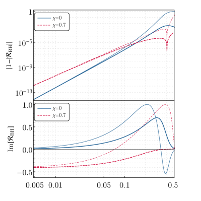
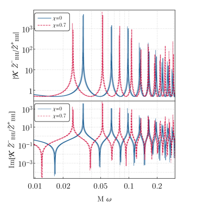
Figure 1: Comparison between our analytical template (thick curves) and the result of a numerical integration of Teukolsky’s equation (thin curves) for $\chi=0$ and $\chi=0.7$. Left panels: the (complex) BH reflection coefficient. Note that the dip in the spinning case corresponds to the threshold of superradiance, i.e. $|{\cal R}_{\rm BH}|^{2}>1$ when $\omega<m\Omega$. Right panels: the absolute value (top) and the imaginary part (bottom) of the ECO response ${\cal K}\tilde{Z}_{\rm BH}^{-}/\tilde{Z}_{\rm BH}^{+}$ as functions of the frequency. For all panels we chose $l=m=2$ and, for the right panels, $\delta/M=10^{-10}$ and ${\cal R}=1$.

III Properties of the template

III.0.1 Comparison with the numerical results

Our analytical template agrees very well with the exact numerical results at low frequency. A representative example is shown in Fig. 1, where we compare the (complex) BH reflection coefficient ${\cal R}_{\rm BH}$ (left panels) and the echo template (right panels) against the result of a numerical integration of Teukolsky’s equation. In the right panels of Fig. 1 we show the quantity ${\cal K}Z_{\rm BH}^{-}$, normalized by the standard BH response $Z_{\rm BH}^{+}$; since $Z_{\rm BH}^{-}$ is proportional to $Z_{\rm BH}^{+}$, the final result is independent of the specific BH response. The agreement (both absolute value and imaginary part) is very good at low frequencies, whereas deviations are present in the transition region where $\omega M\sim 0.1$. Crucially, the low-frequency resonances – which dominate the response Conklin:2017lwb ; Conklin:2019fcs  – are properly reproduced.

Notice that the agreement between analytics and numerics improves as $\delta\to 0$, since the ECO QNMs are at lower frequency (for moderate spin) in this regime and our framework is valid. For technical reasons we were able to produce numerical results up to $\delta=10^{-10}M$, but we expect that the agreement would improve significantly for more realistic (and significantly smaller) values, when $\delta$ is of the order of the Planck length.

To quantify the agreement, we compute the overlap

$${\cal O}=\frac{|\langle\tilde{h}_{A}|\tilde{h}_{N}\rangle|}{\sqrt{|\langle\tilde{h}_{N}|\tilde{h}_{N}\rangle||\langle\tilde{h}_{A}|\tilde{h}_{A}\rangle}|}$$ (30)

between the analytical signal, $\tilde{h}_{A}$, and the numerical one, $\tilde{h}_{N}$, where the inner product is defined as

$$\langle\tilde{X}|\tilde{Y}\rangle\equiv 4\Re\int_{0}^{\infty}\frac{\tilde{X}(f)\tilde{Y}^{*}(f)}{S_{n}(f)}df\,,$$ (31)

(or in a certain frequency range), $S_{n}$ is the detector’s noise spectral density, and $f=\omega/(2\pi)$ is the GW frequency.

When $|{\cal R}|\sim 1$ the presence of very high and narrow resonances makes a quantitative comparison challenging, since a slight displacement of the resonances (due for instance to finite-$\omega$ truncation errors) deteriorates the overlap. For instance, for a representative case shown in Fig. 1 ($\delta=10^{-10}M$, $\chi=0.7$, and ${\cal R}=1$) the overlap is excellent (${\cal O}\gtrsim 0.999$) when the integration is performed before the first resonance, but it quickly reduces to zero after that. To overcome this issue, we compute the overlap in the case in which the resonances are less pronounced, as it is the case when $|{\cal R}|<1$. Let us consider $M=30\,M_{\odot}$, $\chi=0.7$, $\delta=10^{-10}M$, and the aLIGO noise spectral density zerodet . For ${\cal R}=0.9$, the overlap in the range $f\in(20,100)\,{\rm Hz}$ (whose upper end roughly corresponds to the limit $\omega M\sim 0.1$ beyond which the low-frequency approximation is not accurate) is ${\cal O}=0.48$. This small value is mostly due to a small displacement of the resonances. Indeed, by shifting the mass of the analytical waveform by only $1.6\%$, the overlap increases significantly, ${\cal O}=0.995$. For ${\cal R}=0.8$ and in the same conditions, we get ${\cal O}\approx 0.8$ without mass shift and ${\cal O}\gtrsim 0.999$ with the same mass shift as above with the mass shift indicated above. As $\delta\rightarrow 0$, the shift in the mass decreases since the exact resonant frequencies are better reproduced.

III.0.2 Time-domain echo signal: modulation and mixing of the polarizations

The time-domain signal can be computed through an inverse Fourier transform,

$$h(t)=\frac{1}{\sqrt{2\pi}}\int_{-\infty}^{+\infty}d\omega\tilde{Z}^{+}(\omega)e^{-i\omega t}\,,$$ (32)

where $\Re[h(t)]$ and $\Im[h(t)]$ are the two polarizations of the wave, respectively.

In Fig. 2 we present a representative slideshow of our template for different values of $\cal R$ and spins. For simplicity, we consider $\delta/M=10^{-7}$ and ${\cal R(\omega)}={\rm const}$ (but generically complex). The time-domain waveform contains all the features previously reported for the echo signal, in particular amplitude and frequency modulation Cardoso:2016rao ; Cardoso:2016oxy ; Cardoso:2017cqb ; Cardoso:2017njb ; Testa:2018bzd .

In addition, the spin of the object and the phase of the reflectivity coefficient introduce novel effects, such as a nontrivial amplitude modulation of subsequent echoes. This is mostly due to the spin-and-frequency dependence of the phase of ${\cal R}_{\rm BH}$ and ${\cal R}$. The effect of the spin can be seen by comparing the left column ($\chi=0$) of Fig. 2 with the middle ($\chi=0.7$) and the right columns ($\chi=0.9$). Note that the phase of each subsequent echo depends on the combination ${\cal R}{\cal R}_{\rm BH}$, i.e., on the combined action of the reflection by the surface and by the BH barrier. Thus, phase inversion Abedi:2016hgu ; Wang:2018gin ; Testa:2018bzd of each echo relative to the previous one occurs whenever ${\cal R}{\cal R}_{\rm BH}\approx-1$ for low frequencies (cf. Sec. III.0.6 for more details).

Furthermore, note that the first, the second, and the fourth row of Fig. 2 all correspond to perfect reflectivity, $|{\cal R}|=1$, but their echo structure is different: in other words, a phase term in ${\cal R}$ introduces a nontrivial echo pattern. To the best of our knowledge this effect was neglected in the previous analyses.

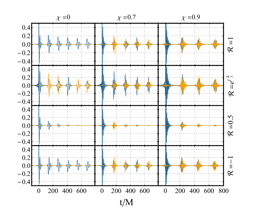
Figure 2: Examples of the gravitational ringdown$+$echo template in the time domain for different values of ${\cal R}(\omega)={\rm const}$, and object’s spin $\chi$. We consider $\delta/M=10^{-7}$. We plot the real (blue curve) and the imaginary (orange curve) parts of the waveform, corresponding to the plus and cross polarization, respectively (note that the ringdown signal is purely plus-polarized, i.e. ${\cal A}_{\times}=0$). Each waveform is normalized to the peak of $|\Re[h(t)]|$ during the ringdown (the peak is not shown in the range of the $y$ axis to better visualize the subsequent echoes). Additional waveforms are provided online webpage .

As shown in Fig. 2 the time-domain signal can contain both plus and cross polarizations, even if the initial ringdown is purely plus polarized (i.e., ${\cal A}_{\times}=0$). This interesting property can be explained as follows. In the nonspinning case, and provided

$${\cal R}_{\chi=0}(\omega)={\cal R}^{*}_{\chi=0}(-\omega^{*})\,,$$ (33)

the transfer function satisfies the symmetry property

$${\cal K}_{\chi=0}(\omega)={\cal K}^{*}_{\chi=0}(-\omega^{*})\,.$$ (34)

The time domain echo waveforms are real (resp., imaginary) if the ringdown waveform is real (resp., imaginary). In this case, the echo signal contains the same polarization of the BH ringdown and the two polarizations do not mix. In particular, Eq. (33) is satisfied when ${\cal R}$ is real.

Remarkably, this property is broken in the following cases:

1. when ${\cal R}$ is complex and does not satisfy Eq. (33) , as in the second row of Fig. 2;

2. generically in the spinning case, even when ${\cal R}$ is real or when it satisfies Eq. (33).

In either case mixing of the polarizations occurs. For instance, if the BH ringdown is (say) a plus-polarized wave (${\cal A}_{\times}=0$), it might acquire a cross-polarization component upon reflection by the photon-sphere barrier (if $\chi\neq 0$) or by the surface (if ${\cal R}$ is complex and does not satisfy Eq. (33)). Therefore, even when the ringdown signal is linearly polarized (as when ${\cal A}_{\times}=0$, the case considered in Fig. 2), generically the final echo signal is not.

The mixing of polarizations can be used to explain the involved echo patter shown in some panels of Fig. 2. For example, for $\chi=0$ and ${\cal R}=e^{i\pi/3}$ each echo is multiplied by $e^{i\pi/3}$ relative to the previous one. Therefore, every three echoes the imaginary part of the signal (i.e., the cross polarization) is zero.

Another interesting consequence of the polarization mixing is the fact that the amplitude of subsequent echoes in each polarization does not decrease monotonically. This is evident, for example, in the panels of Fig. 2 corresponding to $\chi=0.7$, ${\cal R}=1$ and $\chi=0$, ${\cal R}=e^{i\pi/3}$. However, it can be checked that the absolute value of the signal (related to the energy) decreases monotonically.

III.0.3 Decay at late times and superradiant instability

The involved behavior discussed above simplifies at very late times. In this case – when the dominant frequency is roughly $\omega\approx\omega_{R}^{\rm ECO}\ll 1/M$ (where $\omega_{R}^{\rm ECO}$ is the real part of the fundamental QNM of the ECO) – the amplitude of the echoes always decreases as Testa:2018bzd

$$|h_{\rm peaks}(t)|\propto|{\cal R}{\cal R}_{\rm BH}|^{\frac{t}{2|x_{0}|}}\,,$$ (36)

where both ${\cal R}$ and ${\cal R}_{\rm BH}$ are evaluated at $\omega_{R}^{\rm ECO}\ll 1/M$. The above scaling agrees almost perfectly with our time-domain waveforms, especially at late times.

More interestingly, Eq. (36) shows that the signal at late time should grow when $|{\cal R}{\cal R}_{\rm BH}|>1$, i.e., when the combined action of reflection by the surface and by the BH barrier yields an amplification factor larger than unity Maggio:2017ivp ; Maggio:2018ivz . When $|{\cal R}|\approx 1$, this condition requires

$$|{\cal R}_{\rm BH}|>1\,.$$ (37)

From Eq. (21), it is easy to see that this occurs when

$$\omega(\omega-m\Omega)<0\,,$$ (38)

i.e., when the condition for superradiance zeldovich1 ; Teukolsky:1974yv is satisfied (see Ref. Brito:2015oca for an overview). Thus, we expect the signal to grow in time over a time scale given by the ergoregion instability Friedman:1978wla ; Cardoso:2007az ; Cardoso:2008kj ; Brito:2015oca ; Moschidis:2016zjy ; Maggio:2017ivp ; Maggio:2018ivz of spinning horizonless ultracompact objects. Indeed, the QNM spectrum of the object contains unstable modes when $\omega_{R}<m\Omega$ Cardoso:2007az ; Cardoso:2008kj ; Maggio:2017ivp ; Maggio:2018ivz . The instability time scale is always much longer than the dynamical time scale of the object (e.g., $\tau_{\rm instab}\gtrsim 10^{5}M$ for $\chi=0.5$ Maggio:2018ivz ).

When the signal grows in time due to the ergoregion instability the waveform $h(t)$ is a nonintegrable function, so its Fourier transform cannot be defined. For this reason the frequency-domain waveforms are valid up to $t\lesssim\tau_{\rm instab}$. Since the instability time scale is much longer than the echo delay time, the time interval of validity of our waveform still includes a large number of echoes. In particular, the ergoregion instability does not affect the first $N\sim|\log\delta/M|$ echoes LRR .

As discussed in Refs. Maggio:2017ivp ; Maggio:2018ivz , this instability can be quenched if $|{\cal R}{\cal R}_{\rm BH}|<1$, which requires a partially absorbing ECO, $|{\cal R}|<1$ (see Refs. Wang:2019rcf ; Oshita:2019sat for a specific model where the instability is absent).

III.0.4 Energy of echo signal

The energy contained in the ringdown$+$echo signal is shown in Fig. 3, where we plot the quantity

$$E\propto\int_{-\infty}^{\infty}d\omega\,\omega^{2}|\hat{Z}^{+}|^{2}\,,$$ (39)

normalized by the one corresponding to the ringdown alone, $E_{\rm RD}\equiv E({\cal R}=0)$, as a function of the reflectivity ${\cal R}$ and for several values of the spin $\chi$. We use the prescription of Ref. Flanagan:1997sx to compute the ringdown energy, i.e. $\tilde{Z}^{+}_{\rm BH}$ is the frequency-domain full response obtained by using the Fourier transform of

$$Z_{\rm BH}^{+}(t)\sim\mathcal{A}_{+}\,\cos(\omega_{R}t+\phi_{+})e^{-|t|/\tau}\,.$$ (40)

(Notice the absolute value of $t$ at variance with Eq. (23).) This prescription circumvents the problem associated with the Heaviside function in Eq. (23) that produces a spurious high-frequency behavior in the energy flux, leading to infinite energy in the ringdown signal. With the above prescription, the energy defined in Eq. (39) is finite and reduces to the result of Ref. Flanagan:1997sx for the BH ringdown when ${\cal R}=0$.

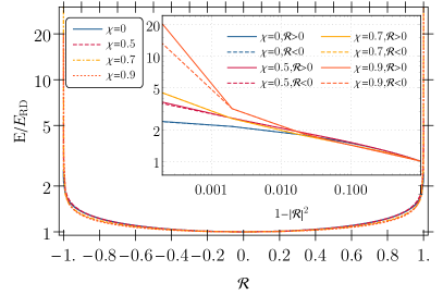
Figure 3: Total energy contained in the ringdown$+$echo signal normalized by that of the ringdown alone as a function of ${\cal R}$ and for various values of the spin $\chi$. The total energy is much larger than the ringdown energy only when ${\cal R}\to 1$. We set $\delta/M=10^{-5}$ and considered only one ringdown polarization with $\phi_{+}=0$; the result is independent of $\delta$ in the $\delta\ll M$ limit.

Because of reflection at the surface, the energy contained in the full signal for a fixed amplitude might be much larger than that of the ringdown itself. Overall, the normalized energy depends mildly on the spin, but much more strongly on ${\cal R}$: the energy contained in the echo part of the signal grows fast as $|{\cal R}|\to 1$ (reaching a maximum value that depends on the spin and might become larger than the energy of the ringdown alone. This is due to the resonances corresponding to the low-frequency QNMs of the ECO, that can be excited with large amplitude Conklin:2017lwb [see bottom panel of Fig. 1], and suggests that GW echoes might be detectable even when the ringdown is not if $|{\cal R}|\approx 1$. However, it is worth noticing that these low-frequency resonances are excited only at late times and therefore the first few echoes contain a small fraction of the total energy of the signal. When ${\cal R}$ is significantly smaller than unity subsequent echoes are suppressed (see third row in Fig. 2) and their total energy is modest compared to that of the ringdown.

Note also that when $|{\cal R}|\approx 1$ the total energy is expected to diverge in the superradiant regime, due to the aforementioned ergoregion instability. This is not captured by the inverse Fourier transform $\hat{Z}^{+}(\omega)$, since the time-domain signal is non-integrable when $t\gtrsim\tau_{\rm instab}$.

III.0.5 Frequency content of the signal

As previously discussed, the photon-sphere barrier acts as a high-pass filter as a consequence of which each echo has a lower frequency content than the previous one. This is confirmed by Fig. 4, where we display the first four echoes for ${\cal R}=1$, $\chi=0$, and $\delta/M=10^{-7}$, shifted in time and rescaled in amplitude so that their global maxima are aligned.

The frequency content of the total signal starts roughly at the BH QNM frequency, and slowly decreases in each subsequent echo until it is dominated by the low-frequency ECO QNMs at very late time. This also shows that a low-frequency approximation becomes increasingly more accurate at later times. In the example shown in Fig. 4, the frequencies of the first four echoes are approximately $M\omega\approx 0.34,0.32,0.3,0.29$, whereas the real part of the fundamental BH QNM for $\chi=0$ is $M\omega_{R}\approx 0.37367$. Therefore, the frequency between the first and the fourth echo decreases by $\approx 17\%$.

Note that the case shown in Fig. 4 is the one that provides the simplest echo patter ($\chi=0$, ${\cal R}\in\Re$). The case $\chi\neq 0$ or a complex choice of ${\cal R}$ would provide a much more involved patter and polarization mixing.

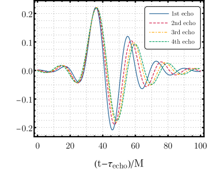
Figure 4: The first four echoes in the time-domain waveform for a model with ${\cal R}=1$, $\chi=0$, $\delta/M=10^{-7}$. The waveform has been shifted in time and rescaled in amplitude so that the global maxima of each echo are aligned. Note that each subsequent echo has a lower frequency content than the previous one.

Our results show that two qualitatively different situations can occur:

• the reflectivity ${\cal R}$ of the object is small enough so that the amplitude of subsequent echoes is suppressed. In this case most of the signal-to-noise ratio (SNR) is contained in the first few echoes at frequency only slightly smaller than the fundamental BH QNM.

• the reflectivity ${\cal R}$ is close to unity, so subsequent echoes are relevant and contribute significantly to the total SNR. In this case the frequency content becomes much smaller than the fundamental BH QNM.

Clearly our low-frequency approximation is expected to be accurate in case B) and less accurate in case A), especially for high spin where $M\omega_{\rm QNM}\sim 0.5$ or larger.

III.0.6 On the phase of the reflectivity coefficients

It is worth remarking that there exist several definitions of the radial function describing the perturbations of a Kerr metric; these are all related to each other by a linear transformation similar to Eq. (5). The BH reflection coefficients that can be defined for each function differ by a phase, while the quantity $|{\cal R}_{\rm BH}|^{2}$ (related to the energy damping/amplification) is invariant Chandra .

The transfer function in Eq. (18) contains both the absolute value and the phase of ${\cal R}_{\rm BH}$. Therefore, one might wonder whether this ambiguity in the phase could affect the ECO response. For a given model, it should be noted that the reflectivity coefficient at the surface, ${\cal R}$, is also affected by the same phase ambiguity, in accordance with the perturbation variable chosen to describe the problem. Since the transfer function depends only on the combinations ${\cal R}{\cal R}_{\rm BH}$ and ${\cal R}{\cal T}_{\rm BH}$, the phase ambiguity in ${\cal R}$ cancels out with that in ${\cal R}_{\rm BH}$ and ${\cal T}_{\rm BH}$ in Eq. (18). This ensures that the transfer function is invariant under the choice of the radial perturbation function, as expected for any measurable quantity. For example, at small frequencies the BH reflection coefficient derived from the asymptotics of the Regge-Wheeler function at $x\to-\infty$ has a phase difference of $\pi$ compared to the BH reflection coefficient computed from the Detweiler function for $\chi=0$. Consistently, the reflectivity coefficient associated to the former differs by a phase $\pi$ with respect to the reflectivity coefficient associated to the latter, i.e., if $\bar{\mathcal{R}}=1$ for Regge-Wheeler then $\bar{\mathcal{R}}=-1$ for Detweiler in the same model, and viceversa.

Therefore, it is natural for ${\cal R}$ to have a nontrivial (and generically frequency- and spin- dependent) phase term, whose expression depends on the formulation of the problem. Obviously, all choices of the radial wavefunctions are equivalent but – for the same ECO model – the complex reflection coefficient ${\cal R}$ should generically be different for each of them. To the best of our knowledge, this point was neglected in actual matched-filtered searches for echoes, which so far considered ${\cal R}$ (and also ${\cal R}_{\rm BH}$) to be real.

This fact is particularly important in light of what previously discussed for the mixing of the polarizations. As shown in the second row of Fig. 2, a phase in ${\cal R}$ introduces a mixing of polarizations for any spin, which results in a more complex shape of the echoes in the individual polarizations of the signal.

Since the phase of ${\cal R}$ depends on the specific ECO model, in the analysis of Sec. IV we will parametrize the reflectivity in a model-agnostic way as ${\cal R}=|{\cal R}|e^{i\phi}$. In principle, both the absolute value and the phase are generically frequency dependent but for simplicity we choose them to be constants or, equivalently, we take the leading-order and low-frequency limit of these quantities. Hence we parametrize our template by $|{\cal R}|$ and $\phi$, different choices of which correspond to different models.

III.0.7 BH QNMs vs ECO QNMs

It is worth considering the inverse-Fourier transform of Eq. (14) (i.e., Eq. (32)) and deform the frequency integral in the complex frequency plane. When ${\cal R}=0$ (i.e., standard BH ringdown) this procedure yields three contributions Leaver:1986gd ; Berti:2009kk : (i) the high-frequency arcs that govern the prompt response, (ii) a sum-over-residues at the poles of the complex frequency plane (defined by $W_{\rm BH}=0=B_{\rm out}$), which correspond to the QNMs and dominate the signal at intermediate times, and (iii) a branch cut on the negative half of the imaginary axis, giving rise to late-time tails due to backscattering off the background curvature.

When ${\cal R}\neq 0$, the pole structure is more involved. The extension of the integral in Eq. (32) to the complex plane contains two types of complex poles: (i) those associated with $\tilde{Z}_{\rm BH}^{+}(\omega)$ ($\sim 1/W_{\rm BH}\sim 1/B_{\rm out}$) and with ${\cal K}\tilde{Z}_{\rm BH}^{-}(\omega)$ ($\sim\mathcal{T}_{\rm BH}/W_{\rm BH}\sim 1/B_{\rm out}^{2}$) which are the standard BH QNMs (but that do not appear in the ECO QNM spectrum Cardoso:2016rao ), and (ii) those associated with the poles of the transfer function ${\cal K}$ (i.e. when ${\cal R}_{\rm BH}={e^{2ikx_{0}}}/{\cal R}$), which correspond to the ECO QNMs.

The late-time signal in the post-merger is dominated by the second type of poles, since the latter have a longer damping time and survive longer. The prompt ringdown is dominated by the first type of poles, i.e., by the dominant QNMs of the corresponding BH spacetime Cardoso:2016rao . Finally, the intermediate region between prompt ringdown and late-time ECO QNM ringing depends on the other parts of the contour integral on the complex plane. As such, they are more complicated to model, since they do not depend on the QNMs alone and might also depend on the source, as in the standard BH case.

IV Projected constraints on ECOs

In this section we use the template derived in Sec. II.7 for a preliminary error estimation of the ECO properties using current and future GW detectors.

The ringdown$+$echo signal displays sharp peaks which originate from the resonances of the transfer function ${\cal K}$ and correspond to the long-lived QNMs of the ECO Maggio:2018ivz . The relative amplitude of each resonance in the signal depends on the source and the dominant modes are not necessarily the fundamental harmonics Mark:2017dnq ; Bueno:2017hyj . We stress that the amplitude of the echo signal depends strongly on the value of ${\cal R}$, especially when $|{\cal R}|\approx 1$. This suggests that the detectability of (or the constraints on) the echoes strongly depends on ${\cal R}$ and would be much more feasible when $|{\cal R}|\approx 1$. Below we quantify this expectation using a Fisher matrix technique, which is accurate at large SNR (see, e.g., Ref. Vallisneri:2007ev ). This is performed as in Ref. Testa:2018bzd , but by including the spin of the object consistently and allowing for a complex reflection coefficient, ${\cal R}=|{\cal R}|e^{i\phi}$.

The Fisher information matrix $\Gamma$ of a template $\tilde{h}(f)$ for a detector with noise spectral density $S_{n}(f)$ reads as

$$\Gamma_{ij}=\langle\partial_{i}\tilde{h}|\partial_{j}\tilde{h}\rangle\,,$$ (41)

where $i,j=1,...,N$, with $N$ being the number of parameters in the template. The SNR $\rho$ is defined such as $\rho^{2}=\langle\tilde{h}|\tilde{h}\rangle$. The covariance matrix, $\Sigma_{ij}$, of the errors on the template’s parameters is the inverse of $\Gamma_{ij}$ and $\sigma_{i}=\sqrt{\Sigma_{ii}}$ (no summation) gives the statistical error associated with the measurement of $i$-th parameter.

We computed numerically the Fisher matrix (41) with our template $\tilde{h}(f)\equiv\tilde{Z}^{+}(f)$ using the sensitivity curves of aLIGO with the design-sensitivity ZERO_DET_high_P zerodet and two configurations for the third-generation (3G) instruments: Cosmic Explorer in the narrow band variant Evans:2016mbw ; Essick:2017wyl , and Einstein Telescope in its ET-D configuration Hild:2010id . We also consider the LISA’s noise spectral density proposed in Ref. LISA . We focus on the most relevant case of gravitational perturbations with $l=m=2$ and consider $M=30\,M_{\odot}$ ($M=10^{6}\,M_{\odot}$) for ground- (space-) based detectors.

As previously discussed, the most generic BH ringdown template contains $7$ parameters (mass, spin, two phases, two amplitudes and starting time). For simplicity, we reduce it to a linearly-polarized ringdown. In particular, we do not include ${\cal A}_{\times}$ and $\phi_{\times}$ in the parameters and inject ${\cal A}_{\times}=0$. This implies that we have $5$ standard-ringdown parameters in our analysis.

The template also depends on two ECO quantities (the frequency-dependent reflection coefficient ${\cal R}(\omega)$ and the parameter $\delta$) which fully characterize the model. The parameter $\delta$ is directly related to physical quantities, in particular, the compactness of the ECO or (equivalently) the redshift at the surface. We parametrize the reflectivity coefficient as

$${\cal R}(\omega)={|{\cal R}|e^{i\phi}}\,,$$ (42)

where $|{\cal R}|$ and $\phi$ are assumed to be frequency independent for simplicity and we remark that $x_{0}=x_{0}(\delta)$ (see Eq. (4)). This yields three ECO parameters: $\delta$, $|{\cal R}|$, and $\phi$.

We consider two cases: (i) a conservative case in which we extract the errors on all the $5+3$ parameters in a Fisher matrix framework and (ii) a more optimistic case in which we assume that the standard-ringdown parameters can be independently and reliably measured through the prompt ringdown, so that we are left with the measurements errors on the $3$ ECO parameters.

IV.1 Conservative case: $5+3$ parameters

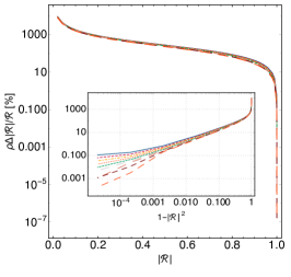
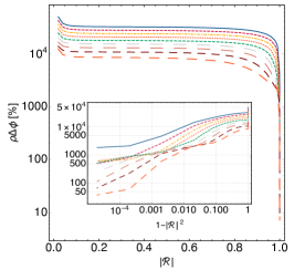
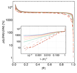
Figure 5: Left panel: relative (percentage) error on the reflection coefficient, $\Delta|{\cal R}|/|{\cal R}|$ multiplied by the SNR, as a function of $|{\cal R}|$ for different values of injected spin. The inset shows the same quantity as a function of $1-|{\cal R}|^{2}$ in a logarithmic scale. From top to bottom: $\chi=(0.9,0.8,0.7,0.6,0.5,0.4,0.3,0.2,0.1)$. Middle panel: same but for the absolute (percentage) error on the phase $\phi$ of ${\cal R}$, i.e. $\rho\Delta\phi$. Right panel: same as in the left panel but for the compactness parameter, $\delta$, i.e. $\Delta(\delta/M)/(\delta/M)$. We assume $\delta=10^{-7}M$ but the errors are independent of $\delta$ when $\delta/M\ll 1$ Testa:2018bzd . We set $\phi=0$ for the phase of ${\cal R}$ (i.e. we consider a real and positive ${\cal R}$, but other choices give very similar results.

Our main results for the statistical errors on the ECO parameters are shown in Fig. 5. In the large SNR limit, the errors scale as $1/\rho$ so we present the quantity $\rho\Delta|{\cal R}|/|{\cal R}|$ (left panel), $\rho\Delta\phi$ (middle panel), and $\rho\Delta(\delta/M)/(\delta/M)$ (right panel) for several values of the spin. We find that the main qualitative features already discussed in Ref. Testa:2018bzd do not depend significantly on the inclusion of the spin in the template. In particular, for fixed SNR the relative errors are almost independent of the specific sensitivity curve of the detector, at least for signals located near each minimum of the sensitivity curve, as those adopted in Fig. 5. In Fig. 5 we adopted the LISA curve LISA but other detectors give very similar results for the errors normalized by the SNR.

Furthermore, the statistical errors are almost independent of $\delta$ when $\delta/M\ll 1$, whereas they strongly depend on the reflection coefficient ${\cal R}$. The reason for this can be again traced back to the presence of resonances as ${\cal R}\to 1$. This feature confirms that it should be relatively straightforward to rule out or detect models with $|{\cal R}|\approx 1$, whereas it is increasingly more difficult to constrain models with smaller values of $|{\cal R}|$.

We also note that the value of the spin of the remnant affects the errors on $|{\cal R}|$ only mildly, whereas it has a stronger impact on the phase of ${\cal R}$ (probably due to the aforementioned mixing of the polarizations) and a moderate impact on the errors on $\delta$.

Overall, the specific value of $\phi$ does not affect the errors significantly, although it is important to include it as an independent parameter in order not to underestimate the errors.

Next, we calculate the SNR necessary to discriminate a partially-absorbing ECO from a BH on the basis of a measurement of ${\cal R}$ at some confidence level Testa:2018bzd . Clearly, if $\Delta{\cal R}/{\cal R}>100\%$, any measurement would be compatible with the BH case (${\cal R}=0$). On the other hand, relative errors $\Delta{\cal R}/{\cal R}<(4.5,0.27,0.007,0.00006)\%$ suggest that it is possible to detect or rule out a given model at $(2,3,4,5)\sigma$ confidence level, respectively. The result of this analysis is shown in Fig. 6, where we present the exclusion plot for the parameter ${\cal R}$ as a function of the SNR in the ringdown phase only, $\rho_{\rm RD}$. Shaded areas represent regions which can be excluded at some given confidence level. Obviously, larger SNRs would allow to probe values of ${\cal R}$ close to the BH limit, ${\cal R}\approx 0$. The extent of the constraints strongly depends on the confidence level. For example, ${\rm SNR\approx 100}$ in the ringdown would allow to distinguish ECOs with $|{\cal R}|^{2}\gtrsim 0.1$ from BHs at $2\sigma$ confidence level, but a $3\sigma$ detection would be possible only if $|{\cal R}|^{2}\gtrsim 0.8$. The reason for this is again related to the strong dependence of the echo signal on ${\cal R}$ . Note that Fig. 6 is very similar to that computed in Ref. Testa:2018bzd , showing that including the spin and a phase term for ${\cal R}$ does not affect the final result significantly.

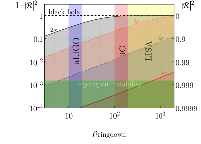
Figure 6: Projected exclusion plot for the ECO reflectivity ${\cal R}$ as a function of the SNR in the ringdown phase. The shaded areas represent regions that can be excluded at a given confidence level ($2\sigma$, $3\sigma$, $4\sigma$, $5\sigma$). Vertical bands are typical SNR achievable by aLIGO/Virgo, 3G, and LISA in the ringdown phase, whereas the horizontal band is the region excluded by the ergoregion instability Maggio:2017ivp ; Maggio:2018ivz . We assumed $\chi=0.7$ for the spin of the merger remnant, the result depends only mildly on the spin.

IV.2 Optimistic case: $3$ ECO parameters

Let us now assume that the standard ringdown parameters (mass, spin, phases, amplitudes, and starting time) can be independently measured through the prompt ringdown signal, which is identical for BHs and ECOs if $\delta/M\ll 1$ Cardoso:2016rao . In such case the remaining three ECO parameters ($|{\cal R}|$, $\phi$, and $\delta$) can be measured a posteriori, assuming the standard ringdown parameters are known.

A representative example for this optimistic scenario is shown in Fig. 7. As expected, the errors are significantly smaller, especially those on the phase $\phi$ of the reflectivity. The errors on ${\cal R}$ are only mildly affected, and the projected constraints on ${\cal R}$ at different confidence levels are similar to those shown in Fig. 6. Nonetheless, we expect this strategy to be much more effective for actual searches.

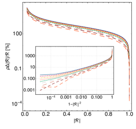
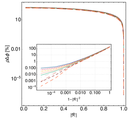
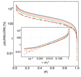
Figure 7: Same as in Fig. 5 but including only the three ECO parameters ($|{\cal R}|$, $\phi$, and $\delta$) in the Fisher analysis.

V Discussion

We have presented an analytical template that describes the ringdown and subsequent echo signal of a spinning, ultracompact, Kerr-like horizonless object. This template depends on the physical parameters of the remnant: namely, the mass, the spin, the compactness and the reflection coefficient ${\cal R}$ at its surface. The analytical approximation is valid at low frequencies, where most of the SNR of an echo signal is accumulated in the case $|{\cal R}|\sim 1$. Our template becomes increasingly accurate at later times as the frequency content of the echo decreases.

The features of the signal are related to the physical properties of the ECO model. The time-domain waveform contains all features previously reported for the echo signal, namely amplitude and frequency modulation and possible phase inversion of each echo relative to the previous one, depending on the reflective boundary conditions. Furthermore, the presence of the spin and of a generically complex reflectivity introduce qualitatively different effects, most notably the amplitude and frequency modulation is more involved (also) due to mixing of the two polarizations. For (almost) perfectly-absorbing spinning ECOs, the perturbations can grow at late times due to superradiance and the ergoregion instability. However, even for highly-spinning remnants, this instability occurs on a time scale which is much longer than the echo delay time, and likely plays a negligible role in actual searches for echoes (see however Ref. Barausse:2018vdb for a discussion of the stochastic background produced by this instability). The instability is quenched for partially-reflecting objects Maggio:2017ivp ; Maggio:2018ivz ; Wang:2019rcf ; Oshita:2019sat .

The amplitude of subsequent echoes depends strongly on the reflectivity ${\cal R}$. When $|{\cal R}|\approx 1$ the echo signal can have energy significantly larger than those of the ordinary BH ringdown. This suggests that GW echoes in certain models might be detectable even when the ringdown is not. Likewise, ruling out models with $|{\cal R}|\approx 1$ is significantly easier than for smaller values of the reflectivity.

We have also highlighted the importance of including a model-dependent phase term in the reflection coefficient; this phase also depends on the radial perturbation variable used in the perturbation equation. To the best of our knowledge this issue has been so far neglected in previous analyses (but see Ref. UchikataEchoes for a recent discussion). We showed that a complex reflectivity at the surface (or, generically, the spin of the remnant) introduce mixing among the two polarizations, drastically modifying the shape of the echoes.

Using a Fisher analysis, we have then estimated the statistical errors on the template parameters for a post-merger GW detection with current and future GW interferometers. Our analysis suggests that ECO models with $|{\cal R}|^{2}\approx 1$ can be detected or ruled out with aLIGO/Virgo (for events with $\rho_{\rm ringdown}\gtrsim 8$) at $5\sigma$ confidence level. These events might also allow us to probe values of the reflectivity as small as $|{\cal R}|^{2}\approx 0.8$ at $\approx 2\sigma$ confidence level.

ECOs with $|{\cal R}|=1$ are already ruled out by the ergoregion instability Cardoso:2008kj ; Maggio:2017ivp and by the absence of GW stochastic background in LIGO O1 run Barausse:2018vdb . Excluding/detecting echoes for models with smaller values of the reflectivity (for which the ergoregion instability is absent Maggio:2017ivp ; Maggio:2018ivz ) requires SNRs in the post-merger phase of ${\cal O}(100)$. This will be achievable only with 3G detectors (ET and Cosmic Explorer) and with the space-based mission LISA. Our preliminary analysis confirms that very stringent constraints on (or detection of) ultracompact horizonless objects can be obtained with current (and especially future) interferometers.

Several interesting extensions of this work are left for the future. In a follow-up paper we plan to adopt the template developed here in a matched-filtered search for GW echoes using LIGO/Virgo public data and for a Bayesian parameter estimation. This can be done for a generic reflectivity coefficient ${\cal R}$, or for specific models, such as those motivated by effective field theory arguments Burgess:2018pmm and the model recently proposed in Refs. Wang:2019rcf ; Oshita:2019sat for the Boltzmann reflectivity of quantum BHs.

An important open problem is to compare the echo template (obtained within perturbation theory) with the post-merger signal of an ECO coalescence producing an echoing merger. Unfortunately, numerical simulations of these systems are currently unavailable and so are inspiral-merger-ringdown waveforms for these models. Assessing the reliability of the analytical template and the importance of nonlinearities will require a comparison between analytical and numerical waveforms, following a path similar to what done in the past for the matching of standard BH ringdown templates with numerical-relativity waveforms (see, e.g., Ref. Buonanno:2006ui ).

A more technical extension deals with the modeling of the signal beyond the low-frequency approximation. The characteristic frequency of the echo signal is always smaller than the corresponding BH ringdown frequency. We expect our template to be robust to the prescription for transition to high frequencies. Nevertheless, it might be interesting to develop a high-frequency analytical approximation of the BH reflection and transmission coefficients to be matched smoothly with a low-frequency approximation. By performing the low-frequency and high-frequency expansions beyond the leading order it might be possible to obtain a better analytical approximation of the transfer function at all frequencies.

Appendix A Low-frequency solution of Teukolsky equation

In this appendix we derive an analytical solution for the reflection coefficient of a BH for gravitational perturbations in the small-frequency regime through a matched asymptotic expansion. The technique is detailed in Ref. Maggio:2018ivz .

For generic spin-$s$ perturbations, Teukolsky’s equations are Teukolsky:1972my ; Teukolsky:1973ha ; Teukolsky:1974yv

$$\Delta^{-s}\frac{d}{dr}\left(\Delta^{s+1}\frac{d_{s}R_{lm}}{dr}\right)$$

$$+ \left[\frac{K^{2}-2is(r-M)K}{\Delta}+4is\omega r-\lambda_{s}\right]\ _{s}R_{lm}=0\,,\quad$$

$$\left[\left(1-y^{2}\right)~{}_{s}S_{lm,y}\right]_{,y}+\bigg{[}(a\omega y)^{2}-2a\omega sy+s$$

$$+ ~{}_{s}A_{lm}-\frac{(m+sy)^{2}}{1-y^{2}}\bigg{]}~{}_{s}S_{lm}=0\,,$$ (44)

where $~{}_{s}S_{lm}(\theta)e^{im\phi}$ are spin-weighted spheroidal harmonics, $y\equiv\cos\theta$, and the separation constants $\lambda$ and $~{}_{s}A_{lm}$ are related by $\lambda_{s}\equiv~{}_{s}A_{lm}+a^{2}\omega^{2}-2am\omega$.

In the region near the surface of the ECO, the radial wave equation (A) for $M\omega\ll 1$ reduces to Starobinskij2

$$\left[z(z+1)\right]^{1-s}\partial_{z}\left\{\left[z(z+1)\right]^{s+1}\partial_{z}R_{s}\right\}$$

$$\quad+\left[Q^{2}+iQs(1+2z)-(l-s)(l+s+1)z(z+1)\right]R_{s}=0\,,$$

(45)

where $z=(r-r_{+})/(r_{+}-r_{-})$ and $R_{s}\equiv~{}_{s}R_{lm}$ for brevity. The general solution of Eq. (45) is a linear combination of hypergeometric functions

$$R_{s} = (1+z)^{iQ}\big{[}{C_{1}}z^{-iQ}$$ (46)

$${}_{2}F_{1}(-l+s,l+1+s;1-\bar{Q}+s;-z)+{C_{2}}z^{iQ-s}$$

$${}_{2}F_{1}(-l+\bar{Q},l+1+\bar{Q};1+\bar{Q}-s;-z)\big{]}\,,$$

where $\bar{Q}=2iQ$ and the integration constants ${C_{1}}$ and ${C_{2}}$ are related to the amplitudes of outgoing and ingoing waves near the surface of the ECO, respectively. For $s=-2$, we transform the solution (46) in the form given by Eq. (5). The near-horizon behavior of the solution is given by Eq. (16), where the coefficients $B_{\text{out}}$ and $B_{\text{in}}$ are related to the integration constants $C_{1}$ and $C_{2}$, respectively.

The large-$r$ behavior of the solution (46) is

$$R_{s} \sim \left(\frac{r}{r_{+}-r_{-}}\right)^{l-s}\Gamma(2l+1)\Bigg{[}\frac{{C_{1}}\ \Gamma(1-\bar{Q}+s)}{\Gamma(l+1-\bar{Q})\Gamma(l+1+s)}$$ (47)

$$+ \frac{{C_{2}}\ \Gamma(1+\bar{Q}-s)}{\Gamma(l+1+\bar{Q})\Gamma(l+1-s)}\Bigg{]}+\left(\frac{r}{r_{+}-r_{-}}\right)^{-l-1-s}$$

$$\frac{(-1)^{l+1+s}}{2\Gamma(2l+2)}\Bigg{[}\frac{{C_{1}}\ \Gamma(l+1-s)\Gamma(1-\bar{Q}+s)}{\Gamma(-l-\bar{Q})}$$

$$+ \frac{{C_{2}}\ \Gamma(l+1+s)\Gamma(1+\bar{Q}-s)}{\Gamma(-l+\bar{Q})}\Bigg{]}\,,$$

At infinity, the radial wave equation (A) for $M\omega\ll 1$ reduces to Cardoso:2008kj

$$r\partial_{r}^{2}f_{s}+2(l+1-i\omega r)\partial_{r}f_{s}-2i(l+1-s)\omega f_{s}=0\,,$$ (48)

where $f_{s}=e^{i\omega r}r^{-l+s}R_{s}$. The general solution of Eq. (48) is a linear combination of a confluent hypergeometric function and a Laguerre polynomial

$$R_{s} = e^{-i\omega r}r^{l-s}\big{[}C_{3}\ U(l+1-s,2l+2,2i\omega r)$$ (49)

$$+ C_{4}\ L_{-l-1+s}^{2l+1}(2i\omega r)\big{]}\,,$$

where the absence of ingoing waves at infinity implies $C_{4}=(-1)^{l-s}\ C_{3}\ \Gamma(-l+s)$. For $s=-2$, the solution (49) is turned in the form given by Eq. (5). In order to have a purely outgoing wave with unitary amplitude at infinity, as in Eq. (16), we impose

$$C_{3}=\frac{(-i\omega)^{1+l}\ 2^{l}\ \Gamma(3+l)}{{\lambda}_{-2}\ {\lambda}_{0}\ \Gamma(-1+l)}\,.$$ (50)

The small-$r$ behavior of the solution (49) is

$$R_{s} \sim C_{3}\ r^{l-s}\frac{(-1)^{l-s}}{2}\frac{\Gamma(l+1+s)}{\Gamma(2l+2)}$$ (51)

$$+ C_{3}\ r^{-l-1-s}(2i\omega)^{-(2l+1)}\frac{\Gamma(2l+1)}{\Gamma(l+1-s)}\,.$$

The matching of Eqs. (47) and (51) in the intermediate region yields

$$\frac{{C_{1}}}{{C_{2}}}=-\frac{\Gamma(l+1+s)}{\Gamma(l+1-s)}\left[\frac{R_{+}+i(-1)^{l}(\omega(r_{+}-r_{-}))^{2l+1}LS_{+}}{R_{-}+i(-1)^{l}(\omega(r_{+}-r_{-}))^{2l+1}LS_{-}}\right]$$ (52)

where

$$R_{\pm} \equiv \frac{\Gamma(1\pm\bar{Q}\mp s)}{\Gamma(l+1\pm\bar{Q})}\,,\quad S_{\pm}\equiv\frac{\Gamma(1\pm\bar{Q}\mp s)}{\Gamma(-l\pm\bar{Q})}\,,$$

$$L \equiv \frac{1}{2}\left[\frac{2^{l}\,\Gamma(l+1+s)\Gamma(l+1-s)}{\Gamma(2l+1)\Gamma(2l+2)}\right]^{2}\,.$$ (53)

The reflection coefficient ${\cal R}_{\rm BH}=B_{\text{in}}/B_{\text{out}}$ is computed in terms of $C_{2}/C_{1}$. By using Eq. (52), we derive an analytical expression for ${\cal R}_{\rm BH}$ at low frequencies. For $l=2$, the equation for ${\cal R}_{\rm BH}$ reads

$${\cal R}_{\rm BH}^{\rm LF}=-8Mke^{\frac{\zeta(\gamma-1)}{\gamma+1}}\frac{2Mk-i(\gamma-1)}{(\gamma-1)^{2}}\left[\frac{-M(\gamma-1)\xi}{L}\right]^{\zeta(\gamma-1)}\left[\frac{16k^{2}M^{2}}{(\gamma-1)^{2}}+1\right]\times$$

$$\frac{\Gamma(-2+\zeta)\Gamma(-1-\zeta)\left[1800i\Gamma(-2-\zeta)+\left(\omega M(\gamma-1)\xi\right)^{5}\Gamma(3-\zeta)\right]}{\Gamma(-2-\zeta)\Gamma(3-\zeta)\left[1800i\Gamma(-2+\zeta)+\left(\omega M(\gamma-1)\xi\right)^{5}\Gamma(3+\zeta)\right]}\,,$$ (54)

where $\gamma=r_{-}/r_{+}$, $\xi=1+\sqrt{1-\chi^{2}}$, $\zeta=i(2\omega M-m\sqrt{\gamma})(\gamma+1)\xi/(\gamma-1)$, and $L$ is an arbitrary constant (with dimensions of a length) which is related to the integration constant of Eq. (7). The expression of ${\cal R}_{\rm BH}$ is provided in a publicly available Mathematica^® notebook webpage .

Appendix B BH response at the horizon in some particular cases

In this appendix we provide some particular case for the BH response at the horizon, $Z_{\rm BH}^{-}$, for some specific toy models of the source. We assume the latter is localized within the cavity.

The simplest case is that of a source localized in space, and for which the frequency dependence can be factored out:

$$\tilde{S}(\omega,x)=C(\omega)\exp\left(-(x-x_{s})^{2}/\sigma^{2}\right)\,,$$ (55)

where $|x_{s}|\ll M$. In this case, it is easy to show that

$$\tilde{\cal Z}_{\rm BH}^{+}=e^{2ikx_{s}}\tilde{Z}_{\rm BH}^{+}\,.$$ (56)

This, together with Eq. (27), yields

$$\tilde{Z}_{\rm BH}^{-}=\left(\frac{e^{2ikx_{s}}+{\cal R}_{\rm BH}}{{\cal T}_{\rm BH}}\right)\tilde{Z}_{\rm BH}^{+}\,.$$ (57)

Remarkably, the above relation is independent of the width of the Gaussian source $\sigma$ and of the function $C(\omega)$ characterizing the source, and it is also valid for any spin. Note that the above result is formally equivalent to the case of localized source studied in Ref. Testa:2018bzd , and in fact reduces to it when $\sigma\to 0$ and $x_{s}$ coincides with the surface location $x_{0}$.

Inspired by Eq. (56), one could also parametrize the BH response $\tilde{\cal Z}_{\rm BH}^{+}$ relative to $\tilde{Z}_{\rm BH}^{+}$ in a model-agnostic way with a generic (complex) proportionality factor:

$$\tilde{\cal Z}_{\rm BH}^{+}=\eta e^{i\nu}Z_{\rm BH}^{+}\,,$$ (58)

where $\eta$ and $\nu$ are (real) parameters of the template. Since the BH response is dominated by the QNMs, a model in which $\tilde{\cal Z}_{\rm BH}^{+}={\cal F}(\omega)Z_{\rm BH}^{+}$ can be effectively reduced to $\tilde{\cal Z}_{\rm BH}^{+}={\cal F}(\omega_{R})Z_{\rm BH}^{+}$. In such case the term ${\cal F}(\omega_{R})=\eta e^{i\nu}$ is a generic parametrization of a complex number.

Finally, another possible model is to consider a plane-wave source that travels towards $\pm\infty$, in this case we have

$$\tilde{S}(x,\omega) = \int dte^{i\omega t}S(x,t)$$ (59)

$$= \int dte^{i\omega t}S(0,t\mp x)=\tilde{S}(0,\omega)e^{\pm i\omega x}\,.$$

Using Eq. (15), we obtain

$$\tilde{Z}_{\rm BH}^{+}(\omega)=\tilde{Z}_{\rm BH}^{-}(\omega)\frac{\int_{-\infty}^{+\infty}dx\Psi_{-}e^{\pm i\omega x}}{\int_{-\infty}^{+\infty}dx\Psi_{+}e^{\pm i\omega x}}\,,$$ (60)

or, more explicitly

$$\tilde{Z}_{\rm BH}^{+}(\omega)=\tilde{Z}_{\rm BH}^{-}(\omega)\frac{\int_{{x\sim 0}}dx\Psi_{-}e^{i\omega x}+\int^{\infty}(A_{\textrm{out}}e^{2i\omega x}+A_{\textrm{in}})dx+\int_{-\infty}dxe^{im\Omega x}}{\int_{x\sim 0}dx\Psi_{+}e^{i\omega x}+\int^{\infty}e^{2i\omega x}dx+\int_{-\infty}(B_{\textrm{out}}e^{2i\omega x-im\Omega x}+B_{\textrm{in}}e^{im\Omega x})dx\,,}\,,$$

where ${x\sim 0}$ is the region where the potential is non-zero and we considered only the upper-sign case for ease of notation. Considering that $\tilde{Z}_{\rm BH}^{+}(\omega)$ has a pole at $\omega_{\rm QNM}=\omega_{R}+i\omega_{I}$ we expect also $\tilde{Z}_{\rm BH}^{-}(\omega)$ to have such a pole. Since $\Im\omega_{\rm QNM}<0$ the terms $\int^{+\infty}dx$ dominate the numerator and the denominator for $\omega\approx\omega_{\rm QNM}$, and we obtain

$$\tilde{Z}_{\rm BH}^{+}\approx-\left(\frac{\mathcal{R}_{\rm BH}}{\mathcal{T}_{\rm BH}}\right)^{*}\tilde{Z}_{\rm BH}^{-}\,.$$ (61)

The case with the lower sign (plane wave traveling toward $-\infty$) gives the same result.

References

- (1) V. Cardoso, E. Franzin, and P. Pani, “Is the gravitational-wave ringdown a probe of the event horizon?,” Phys. Rev. Lett. 116 no. 17, (2016) 171101, arXiv:1602.07309 [gr-qc].
- (2) V. Cardoso, S. Hopper, C. F. B. Macedo, C. Palenzuela, and P. Pani, “Gravitational-wave signatures of exotic compact objects and of quantum corrections at the horizon scale,” Phys. Rev. D94 no. 8, (2016) 084031, arXiv:1608.08637 [gr-qc].
- (3) N. Oshita and N. Afshordi, “Probing microstructure of black hole spacetimes with gravitational wave echoes,” Phys. Rev. D99 no. 4, (2019) 044002, arXiv:1807.10287 [gr-qc].
- (4) Q. Wang, N. Oshita, and N. Afshordi, “Echoes from Quantum Black Holes,” arXiv:1905.00446 [gr-qc].
- (5) V. Ferrari and K. D. Kokkotas, “Scattering of particles by neutron stars: Time evolutions for axial perturbations,” Phys. Rev. D62 (2000) 107504, arXiv:gr-qc/0008057 [gr-qc].
- (6) P. Pani and V. Ferrari, “On gravitational-wave echoes from neutron-star binary coalescences,” Class. Quant. Grav. 35 no. 15, (2018) 15LT01, arXiv:1804.01444 [gr-qc].
- (7) L. Buoninfante and A. Mazumdar, “Nonlocal star as a blackhole mimicker,” arXiv:1903.01542 [gr-qc].
- (8) L. Buoninfante, A. Mazumdar, and J. Peng, “Nonlocality amplifies echoes,” arXiv:1906.03624 [gr-qc].
- (9) A. Delhom, C. F. B. Macedo, G. J. Olmo, and L. C. B. Crispino, “Absorption by black hole remnants in metric-affine gravity,” arXiv:1906.06411 [gr-qc].
- (10) V. Cardoso and P. Pani, “Tests for the existence of black holes through gravitational wave echoes,” Nat. Astron. 1 no. 9, (2017) 586–591, arXiv:1709.01525 [gr-qc].
- (11) V. Cardoso and P. Pani, “The observational evidence for horizons: from echoes to precision gravitational-wave physics,” arXiv:1707.03021 [gr-qc].
- (12) V. Cardoso and P. Pani, “Testing the nature of dark compact objects: a status report,” arXiv:1904.05363 [gr-qc].
- (13) J. Abedi, H. Dykaar, and N. Afshordi, “Echoes from the Abyss: Tentative evidence for Planck-scale structure at black hole horizons,” Phys. Rev. D96 no. 8, (2017) 082004, arXiv:1612.00266 [gr-qc].
- (14) R. S. Conklin, B. Holdom, and J. Ren, “Gravitational wave echoes through new windows,” Phys. Rev. D98 no. 4, (2018) 044021, arXiv:1712.06517 [gr-qc].
- (15) J. Abedi and N. Afshordi, “Echoes from the Abyss: A highly spinning black hole remnant for the binary neutron star merger GW170817,” arXiv:1803.10454 [gr-qc].
- (16) G. Ashton, O. Birnholtz, M. Cabero, C. Capano, T. Dent, B. Krishnan, G. D. Meadors, A. B. Nielsen, A. Nitz, and J. Westerweck, “Comments on: ”Echoes from the abyss: Evidence for Planck-scale structure at black hole horizons”,” arXiv:1612.05625 [gr-qc].
- (17) J. Abedi, H. Dykaar, and N. Afshordi, “Echoes from the Abyss: The Holiday Edition!,” arXiv:1701.03485 [gr-qc].
- (18) J. Westerweck, A. Nielsen, O. Fischer-Birnholtz, M. Cabero, C. Capano, T. Dent, B. Krishnan, G. Meadors, and A. H. Nitz, “Low significance of evidence for black hole echoes in gravitational wave data,” Phys. Rev. D97 no. 12, (2018) 124037, arXiv:1712.09966 [gr-qc].
- (19) J. Abedi, H. Dykaar, and N. Afshordi, “Comment on: ”Low significance of evidence for black hole echoes in gravitational wave data”,” arXiv:1803.08565 [gr-qc].
- (20) N. Uchikata, H. Nakano, T. Narikawa, N. Sago, H. Tagoshi, and T. Tanaka, “Searching for black hole echoes from the LIGO-Virgo Catalog GWTC-1,” arXiv:1906.00838 [gr-qc].
- (21) K. W. Tsang, A. Ghosh, A. Samajdar, K. Chatziioannou, S. Mastrogiovanni, M. Agathos, and C. V. D. Broeck, “A morphology-independent search for gravitational wave echoes in data from the first and second observing runs of Advanced LIGO and Advanced Virgo,” arXiv:1906.11168 [gr-qc].
- (22) R. S. Conklin and B. Holdom, “Gravitational Wave ”Echo” Spectra,” arXiv:1905.09370 [gr-qc].
- (23) K. W. Tsang, M. Rollier, A. Ghosh, A. Samajdar, M. Agathos, K. Chatziioannou, V. Cardoso, G. Khanna, and C. Van Den Broeck, “A morphology-independent data analysis method for detecting and characterizing gravitational wave echoes,” Phys. Rev. D98 no. 2, (2018) 024023, arXiv:1804.04877 [gr-qc].
- (24) K. Lin, W.-L. Qian, X. Fan, and H. Zhang, “Tail wavelets in the merger of binary compact objects,” arXiv:1903.09039 [gr-qc].
- (25) H. Nakano, N. Sago, H. Tagoshi, and T. Tanaka, “Black hole ringdown echoes and howls,” PTEP 2017 no. 7, (2017) 071E01, arXiv:1704.07175 [gr-qc].
- (26) Z. Mark, A. Zimmerman, S. M. Du, and Y. Chen, “A recipe for echoes from exotic compact objects,” arXiv:1706.06155 [gr-qc].
- (27) A. Maselli, S. H. Volkel, and K. D. Kokkotas, “Parameter estimation of gravitational wave echoes from exotic compact objects,” Phys. Rev. D96 no. 6, (2017) 064045, arXiv:1708.02217 [gr-qc].
- (28) P. Bueno, P. A. Cano, F. Goelen, T. Hertog, and B. Vercnocke, “Echoes of Kerr-like wormholes,” Phys. Rev. D97 no. 2, (2018) 024040, arXiv:1711.00391 [gr-qc].
- (29) Y.-T. Wang, Z.-P. Li, J. Zhang, S.-Y. Zhou, and Y.-S. Piao, “Are gravitational wave ringdown echoes always equal-interval?,” Eur. Phys. J. C78 no. 6, (2018) 482, arXiv:1802.02003 [gr-qc].
- (30) M. R. Correia and V. Cardoso, “Characterization of echoes: A Dyson-series representation of individual pulses,” Phys. Rev. D97 no. 8, (2018) 084030, arXiv:1802.07735 [gr-qc].
- (31) Q. Wang and N. Afshordi, “Black hole echology: The observer’s manual,” Phys. Rev. D97 no. 12, (2018) 124044, arXiv:1803.02845 [gr-qc].
- (32) A. Testa and P. Pani, “Analytical template for gravitational-wave echoes: signal characterization and prospects of detection with current and future interferometers,” Phys. Rev. D98 no. 4, (2018) 044018, arXiv:1806.04253 [gr-qc].
- (33) J. L. Friedman, “Ergosphere instability,” Communications in Mathematical Physics 63 (Oct., 1978) 243–255.
- (34) G. Moschidis, “A Proof of Friedman’s Ergosphere Instability for Scalar Waves,” Commun. Math. Phys. 358 no. 2, (2018) 437–520, arXiv:1608.02035 [math.AP].
- (35) R. Brito, V. Cardoso, and P. Pani, “Superradiance,” Lect. Notes Phys. 906 (2015) pp.1–237, arXiv:1501.06570 [gr-qc].
- (36) V. Cardoso, P. Pani, M. Cadoni, and M. Cavaglia, “Ergoregion instability of ultracompact astrophysical objects,” Phys. Rev. D77 (2008) 124044, arXiv:0709.0532 [gr-qc].
- (37) V. Cardoso, P. Pani, M. Cadoni, and M. Cavaglia, “Instability of hyper-compact Kerr-like objects,” Class. Quant. Grav. 25 (2008) 195010, arXiv:0808.1615 [gr-qc].
- (38) C. B. M. H. Chirenti and L. Rezzolla, “On the ergoregion instability in rotating gravastars,” Phys. Rev. D78 (2008) 084011, arXiv:0808.4080 [gr-qc].
- (39) V. Cardoso, L. C. B. Crispino, C. F. B. Macedo, H. Okawa, and P. Pani, “Light rings as observational evidence for event horizons: long-lived modes, ergoregions and nonlinear instabilities of ultracompact objects,” Phys. Rev. D90 no. 4, (2014) 044069, arXiv:1406.5510 [gr-qc].
- (40) E. Maggio, P. Pani, and V. Ferrari, “Exotic Compact Objects and How to Quench their Ergoregion Instability,” Phys. Rev. D96 no. 10, (2017) 104047, arXiv:1703.03696 [gr-qc].
- (41) E. Maggio, V. Cardoso, S. R. Dolan, and P. Pani, “Ergoregion instability of exotic compact objects: electromagnetic and gravitational perturbations and the role of absorption,” Phys. Rev. D99 no. 6, (2019) 064007, arXiv:1807.08840 [gr-qc].
- (42) R. Vicente, V. Cardoso, and J. C. Lopes, “Penrose process, superradiance, and ergoregion instabilities,” Phys. Rev. D97 no. 8, (2018) 084032, arXiv:1803.08060 [gr-qc].
- (43) E. Barausse, R. Brito, V. Cardoso, I. Dvorkin, and P. Pani, “The stochastic gravitational-wave background in the absence of horizons,” Class. Quant. Grav. 35 no. 20, (2018) 20LT01, arXiv:1805.08229 [gr-qc].
- (44) G. Poschl and E. Teller, “Bemerkungen zur Quantenmechanik des anharmonischen Oszillators,” Z. Phys. 83 (1933) 143–151.
- (45) V. Ferrari and B. Mashhoon, “New approach to the quasinormal modes of a black hole,” Phys. Rev. D30 (1984) 295–304.
- (46) http://www.darkgra.org.
- (47) G. Raposo, P. Pani, and R. Emparan, “Exotic compact objects with soft hair,” arXiv:1812.07615 [gr-qc].
- (48) C. Barcelo, R. Carballo-Rubio, and S. Liberati, “Generalized no-hair theorems without horizons,” arXiv:1901.06388 [gr-qc].
- (49) P. Pani, “I-Love-Q relations for gravastars and the approach to the black-hole limit,” Phys. Rev. D92 no. 12, (2015) 124030, arXiv:1506.06050 [gr-qc].
- (50) N. Uchikata and S. Yoshida, “Slowly rotating thin shell gravastars,” Class. Quant. Grav. 33 no. 2, (2016) 025005, arXiv:1506.06485 [gr-qc].
- (51) N. Uchikata, S. Yoshida, and P. Pani, “Tidal deformability and I-Love-Q relations for gravastars with polytropic thin shells,” Phys. Rev. D94 no. 6, (2016) 064015, arXiv:1607.03593 [gr-qc].
- (52) K. Yagi and N. Yunes, “I-Love-Q anisotropically: Universal relations for compact stars with scalar pressure anisotropy,” Phys. Rev. D91 no. 12, (2015) 123008, arXiv:1503.02726 [gr-qc].
- (53) K. Yagi and N. Yunes, “Relating follicly-challenged compact stars to bald black holes: A link between two no-hair properties,” Phys. Rev. D91 no. 10, (2015) 103003, arXiv:1502.04131 [gr-qc].
- (54) C. Posada, “Slowly rotating supercompact Schwarzschild stars,” Mon. Not. Roy. Astron. Soc. 468 no. 2, (2017) 2128–2139, arXiv:1612.05290 [gr-qc].
- (55) S. A. Teukolsky, “Rotating black holes - separable wave equations for gravitational and electromagnetic perturbations,” Phys. Rev. Lett. 29 (1972) 1114–1118.
- (56) S. A. Teukolsky, “Perturbations of a rotating black hole. 1. Fundamental equations for gravitational electromagnetic and neutrino field perturbations,” Astrophys. J. 185 (1973) 635–647.
- (57) S. A. Teukolsky and W. H. Press, “Perturbations of a rotating black hole. III - Interaction of the hole with gravitational and electromagnet ic radiation,” Astrophys. J. 193 (1974) 443–461.
- (58) S. Detweiler, “On resonant oscillations of a rapidly rotating black hole,” Proceedings of the Royal Society of London Series A 352 (July, 1977) 381–395.
- (59) S. Chandrasekhar, The Mathematical Theory of Black Holes. Oxford University Press, New York, 1983.
- (60) A. Vilenkin, “Exponential Amplification of Waves in the Gravitational Field of Ultrarelativistic Rotating Body,” Phys. Lett. B78 (1978) 301–303.
- (61) I. Novikov and V. Frolov, Black Hole Physics. Springer, 1989.
- (62) M. Casals and A. C. Ottewill, “Canonical quantization of the electromagnetic field on the kerr background,” Phys. Rev. D 71 (Jun, 2005) 124016. https://link.aps.org/doi/10.1103/PhysRevD.71.124016.
- (63) A. A. Starobinskij and S. M. Churilov, “Amplification of electromagnetic and gravitational waves scattered by a rotating black hole.,” Zhurnal Eksperimentalnoi i Teoreticheskoi Fiziki 65 (1973) 3–11.
- (64) A. Neitzke, “Greybody factors at large imaginary frequencies,” arXiv:hep-th/0304080 [hep-th].
- (65) T. Harmark, J. Natario, and R. Schiappa, “Greybody Factors for d-Dimensional Black Holes,” Adv. Theor. Math. Phys. 14 no. 3, (2010) 727–794, arXiv:0708.0017 [hep-th].
- (66) E. Berti, V. Cardoso, and C. M. Will, “On gravitational-wave spectroscopy of massive black holes with the space interferometer LISA,” Phys. Rev. D73 (2006) 064030, arXiv:gr-qc/0512160 [gr-qc].
- (67) A. Buonanno, G. B. Cook, and F. Pretorius, “Inspiral, merger and ring-down of equal-mass black-hole binaries,” Phys. Rev. D75 (2007) 124018, arXiv:gr-qc/0610122 [gr-qc].
- (68) N. Oshita, Q. Wang, and N. Afshordi, “On Reflectivity of Quantum Black Hole Horizons,” arXiv:1905.00464 [hep-th].
- (69) LIGO Collaboration, D. Shoemaker, “Advanced ligo anticipated sensitivity curves,” Tech. Rep. T0900288-v3, 2010. https://dcc.ligo.org/LIGO-T0900288/public.
- (70) Y. B. Zel’dovich Pis’ma Zh. Eksp. Teor. Fiz. 14 (1971) 270 [JETP Lett. 14, 180 (1971)].
- (71) J. L. Friedman, “Generic instability of rotating relativistic stars,” Commun. Math. Phys. 62 no. 3, (1978) 247–278.
- (72) E. E. Flanagan and S. A. Hughes, “Measuring gravitational waves from binary black hole coalescences: 1. Signal-to-noise for inspiral, merger, and ringdown,” Phys. Rev. D57 (1998) 4535–4565, arXiv:gr-qc/9701039 [gr-qc].
- (73) E. W. Leaver, “Spectral decomposition of the perturbation response of the Schwarzschild geometry,” Phys. Rev. D34 (1986) 384–408.
- (74) E. Berti, V. Cardoso, and A. O. Starinets, “Quasinormal modes of black holes and black branes,” Class. Quantum Grav. 26 (2009) 163001, arXiv:0905.2975 [gr-qc].
- (75) M. Vallisneri, “Use and abuse of the Fisher information matrix in the assessment of gravitational-wave parameter-estimation prospects,” Phys. Rev. D77 (2008) 042001, arXiv:gr-qc/0703086 [GR-QC].
- (76) LIGO Scientific Collaboration, B. P. Abbott et al., “Exploring the Sensitivity of Next Generation Gravitational Wave Detectors,” Class. Quant. Grav. 34 no. 4, (2017) 044001, arXiv:1607.08697 [astro-ph.IM].
- (77) R. Essick, S. Vitale, and M. Evans, “Frequency-dependent responses in third generation gravitational-wave detectors,” Phys. Rev. D96 no. 8, (2017) 084004, arXiv:1708.06843 [gr-qc].
- (78) S. Hild et al., “Sensitivity Studies for Third-Generation Gravitational Wave Observatories,” Class. Quant. Grav. 28 (2011) 094013, arXiv:1012.0908 [gr-qc].
- (79) H. Audley, S. Babak, J. Baker, E. Barausse, P. Bender, E. Berti, P. Binetruy, M. Born, D. Bortoluzzi, J. Camp, C. Caprini, V. Cardoso, M. Colpi, J. Conklin, N. Cornish, C. Cutler, et al., “Laser Interferometer Space Antenna,” ArXiv e-prints (Feb., 2017) , arXiv:1702.00786 [astro-ph.IM].
- (80) C. P. Burgess, R. Plestid, and M. Rummel, “Effective Field Theory of Black Hole Echoes,” JHEP 09 (2018) 113, arXiv:1808.00847 [gr-qc].