From Planck area to graph theory:
Topologically distinct black hole microstates

Abstract

We postulate a Planck scale horizon unit area, with no bits of information locally attached to it, connected but otherwise of free form, and let $n$ such geometric units compactly tile the black hole horizon. Associated with each topologically distinct tiling configuration is then a simple, connected, undirected, unlabeled, planar, chordal graph. The asymptotic enumeration of the corresponding integer sequence gives rise to the Bekenstein-Hawking area entropy formula, automatically accompanied by a proper logarithmic term, and fixes the size of the horizon unit area, thereby constituting a global realization of Wheeler’s ”it from bit” phrase. Invoking Polya’s theorem, an exact number theoretical entropy spectrum is offered for the 2+1 dimensional quantum black hole.

I I. Introduction

The semiclassical Bekenstein-Hawking black hole area entropy formula BH

$$S_{BH}=k_{B}\frac{A_{BH}}{4\ell_{P}^{2}}~{},$$ (1)

governed by the horizon surface area $A_{BH}$, measured in Planck units $\ell_{P}^{2}=G\hbar/c^{3}$, and factorized by the Boltzmann constant $k_{B}$, is still as mysterious as ever. We have no compelling answer for what the physical degrees of freedom underlying the Schwarzschild black hole prototype actually are, or for how to identify and count its elusive quantum microstates. Various attempts to address this issue have come from all corners of theoretical physics, way beyond general relativity, including string theory string , loop quantum gravity loop , and AdS/CFT AdSCFT , each theory contributing its inimitable insight. According to Maldacena Malda , ”these microstates do not have an explicit calculable description within the regime that gravity is a good approximation.”

It was Bekenstein nA who first realized that the black hole surface area may serve as a classical adiabatic invariant, and as such, it must exhibit a discrete ladder spectrum of the form $A_{BH}(n)=nA_{1}$. This has opened the door for a variety of Bekenstein-Mukhanov BM inspired quantum black hole models models , the majority of which assume $\gamma$ (a natural number) bits of information locally encoded in each Planck area on the horizon. Such a local realization of Wheeler’s ’it from bit’ phrase Wh gives rise to a total of $g(n)=\gamma^{n}$ configurations. However, no compelling clue was given as to what these bits actually stand for or what physics is capable of hosting them on the event horizon. Along these lines, it is worth recalling the ’t Hooft-Susskind holographic principle holo which asserts that all of the information contained in some closed region of space, saturated by Eq.(1), can in fact be represented as a hologram on the boundary of that region.

While the general idea of a fundamental Planck scale horizon unit area is not new, the role it plays in the present model is novel. In fact, in contrast to almost all Bekenstein-Mukhanov- type models, no bits of information are locally attached to any single unit area. An individual Planck area does not play any local role at all here. Alternatively, our interest is focused on a collective mode of all Planck units involved, with the various topologically distinguished configurations highly resembling (and perhaps identified as) the quantum black hole microstates. Their counting, and the subsequent recovery of Eq.(1) in the semiclassical limit, which is automatically accompanied by a proper logarithmic term, is carried out by invoking graph theoretical enumeration. Triggered by graph theory, the black hole discrete entropy spectrum is furthermore shown to establish a serendipitous link with number theory (with the focus on Polya’s theorem Polya ).

II II. Horizon tiling

The main ingredient in our quantum black hole model is a postulated Planck size horizon unit area

$$A_{P}=\eta\ell_{P}^{2}$$ (2)

where $\eta$ is a dimensionless universal constant, which is eventually fixed by means of graph theory. Eq.(2) may further serve as a geometric lower bound inspired by the ’t Hooft-Susskind holographic principle holo , but this is beyond the scope of the present model. Based on self-consistency grounds, the Planck unit area must exhibit a locally connected structure but can otherwise take any free form. Its boundary can thus undergo any arbitrary variation as long as the size of the surrounding area is preserved in accordance with Eq.(2).

We now attempt to compactly tile the black hole horizon surface area $A_{BH}$ by exactly

$$n=\frac{A_{BH}}{A_{P}}$$ (3)

elementary Planck unit areas. It makes no sense, and actually there is no option, to perform this uniformly. The reason is quite obvious: While Planck unit areas are all topologically equivalent, they may still differ from each other by acquiring arbitrary, albeit connected, shapes. For any given integer number $n$ of Planck unit areas, the relevant question is then how many topologically distinct tiling configurations $g(n)$ actually exist?

Counting configurations calls for graph theory enumeration. The first step is to show, by construction, that associated with each topologically distinct tiling configuration is a certain mathematical graph, defined as a set of vertices connected by edges. There are four simple instructions:

1. Assign a graph vertex to each Planck unit area, and locate this vertex at some point on that unit (this is always possible due to the local connectedness).

2. Connect any two such vertices by a graph edge if and only if the two corresponding Planck unit areas touch each other.

3. Draw the graph on the horizon itself, and take into account the fact that from the topological point of view, as a 2-dimensional spherical surface $S^{2}$ with no handles, the Schwarzschild horizon is of genus $0$. This is a guaranteed by Hawking theorem Hawking which holds for asymptotically flat 4-dimensional black holes obeying the dominant energy condition. Genus dependence will be briefly discussed later.

4. By choosing one graph face and puncturing a hole in it, one may further, via a stereographic projection, reliably transform the graph from the sphere onto a plane. The punctured face on the sphere becomes the exterior face on the plane.

The transition from the black hole horizon tiling to graph theory is demonstrated in Fig.1 for $n=4$ vertices.

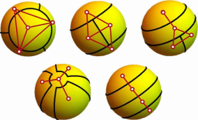
Figure 1: Translating horizon tiling into graph theory language. The demonstration is carried out for $n=4$ deformable Planck unit areas (separated by black borders), resulting in $g(4)=5$ topologically distinct configurations. Associated with each such configuration is a simple, connected, undirected, unlabeled, planar, chordal graph (plotted in red).

III III. Graph theory

Prior to performing enumeration, we must accurately specify what kind of graphs we are actually dealing with. By construction, mostly on geometric or physical grounds, these graphs must be as follows:

1. Simple. - The graph cannot contain loops and/or multiple edges. A Planck area unit does not touch itself, and it is clear whether or not two Planck areas share a common border.

2. Connected. - There must be a path from any vertex to any other vertex of the graph. Allowing for a disconnected graph, an isolated Planck area unit for example, would mean leaving a region of

3. Undirected. - No flow is described in the model. In turn, no arrows need to be attached to the graph edges.

4. Unlabeled. - Reflecting the fact that individual Planck areas have no distinct identifications except through their interconnectivity, the graph vertices do not carry any serial numbers. As we shall see, this is the strongest requirement on our list. On the practical side, it is much harder to enumerate unlabeled than labeled graphs.

5. Planar. - A graph is planar if it can be drawn in a plane, or on a handle-free sphere like the horizon, without graph edges crossing. Be aware that (i) fake edge crossings can be removed by replacing straight lines by Jordan arcs, and (ii) there may be several representations of the same planar graph. For any given number $n$ of nodes, the number of labeled planar graphs turns out to be much larger than the number of unlabeled planar graphs since almost all planar graphs have a large automorphism group.

6. Chordal. - A chordal graph, also called a triangulated graph, is a simple graph in which every cycle of more than three vertices has a chord ($=$ an edge that is not part of the cycle but connects two vertices of the cycle). Beware that chordality is sometimes visually hidden. To see why this is relevant for our case, let four Planck areas meet at some point on the horizon. However, such a configuration turns out, to be topologically unstable with respect to small variations in the shapes of the Planck areas involved. Roughly speaking, a 4-meeting point easily bifurcates into two 3-meeting neighboring points, which is translated into graph theory as adding a chord. The corresponding disqualification of the square graph is illustrated for $n=4$ in Fig.2. To sharpen the genus dependence, note that when plotted on a torus (genus $1$), rather than on a sphere (genus $0$), the square graph becomes stable and thus permissible.

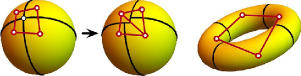
Figure 2: The 4-edge square graph, representing a truncated (cutoff poles) beach ball, is excluded. The 4-meeting point on the ball is unstable against small shape variations of the horizon unit areas, bifurcating into two 3-meeting points. This is translated into graph theory as adding a chord. On a torus, as a counterexample, the square graph is permissible.

Altogether, the above list of graphic features homes in on a particular integer sequence classified as OEIS A243787. To be more explicit, the first terms of the series (so far, only the first 14 terms have been calculated Huffner ) are given by

$$g(n)=1,1,2,5,14,52,228,1209,...$$ (4)

(See Fig.3 for the graphs associated with the first terms.) It starts like the Catalan series, but then grows faster. For comparison, had we given up the chordality requirement, we would end up with a much larger set

$$g_{u}(n)=1,1,2,6,20,99,646,5974,...$$ (5)

of unlabeled connected planar graphs. Clearly, the former Eq.(4) is a subsequence of the latter Eq.(5).

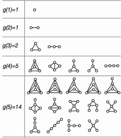
Figure 3: The integer sequence OEIS A243787: Simple, connected, undirected, unlabeled, planar, chordal graphs with $n$ nodes. The inner structure of these graphs is solely composed of triangles and trees. In our model, each graph represents a topologically distinct black hole microstate.

Treating all topologically distinct configurations on equal footing, with each individual configuration serving as a distinct quantum mechanical microstate, the statistical black hole entropy is given by the Boltzmann formula

$$S_{BH}=k_{B}\log g(n)~{}.$$ (6)

As anticipated, the lightest Schwarzschild black hole, carrying mass $m_{1}=m_{P}\sqrt{\eta/16\pi}$, comes with a vanishing entropy $S_{1}=0$. The nontrivial microstate degeneracy starts at $n=3$. An exact analytic formula for $g(n)$ is still unknown, but some efficient enumeration algorithms do exist. However, at this stage, this is not what really matters. Bearing in mind that the fate of our model primarily depends on making contact with Eq.(1) at the large-$n$ semiclassical limit, we content ourselves with an asymptotic enumeration formula.

IV IV. Asymptotic enumeration

Counting labeled planar graphs appears to be much easier than counting planar unlabeled graphs. The asymptotic number $g_{l}(n)$ of labeled planar graphs has been shown, following a superadditivity argument McDiarmid , to obey the limit

$$\lim_{n\to\infty}(g_{l}(n)/n!)^{1/n}\rightarrow\gamma_{l}~{}.$$ (7)

Upper as well as lower bounds on the constant $\gamma_{l}$ were numerically derived, but the final word was given analytically by Gimenez and Noy Noy . To be more specific, they calculated

$$g_{l}(n)\simeq\alpha_{l}n^{-\frac{7}{2}}\gamma_{l}^{n}n!~{},$$ (8)

where $\alpha_{l}\simeq 0.4310^{-5}$ and $\gamma_{l}\simeq 27.23$. As far as the unlabeled planar graphs are concerned, owing to their large exponential number of automorphisms, the limit on the corresponding asymptotic number $g_{u}(n)$ of configurations is conceptually different. In fact, it has been shown Denise that

$$\lim_{n\to\infty}g_{u}(n)^{1/n}\rightarrow\gamma_{u}~{},$$ (9)

thereby consistently defining $\gamma_{u}$ as the unlabeled planar graph growth constant. Notice that, in comparison with Eq.(7), the $n!$ factor is gone. In turn, with Eq.(6) in mind, the leading linear $n$ behavior of $\log g_{u}(n)\simeq n\log\gamma_{u}$ is crucial for ouir model, to be contrasted with the problematic (for our needs) leading behavior of $\log g_{l}(n)\simeq n\log n$. Apart from the $n!$ factor, the asymptotic enumeration of unlabeled planar graphs cannot be too different analytically from that of labeled planer graphs. Thus it comes with no surprise that, in analogy with Eq.(8), Gimenez and Noy have derived

$$g_{u}(n)\simeq\alpha_{u}n^{-\frac{7}{2}}\gamma_{u}^{n}~{},$$ (10)

for some $\alpha_{u},\gamma_{u}$. At this stage, while the exact value of $\gamma_{u}$ is still unknown, Bonichon at al. Bonichon have closed the range to $27.23<\gamma_{u}<30.06$.

For the sake of enumeration, it is useful to probe the inner structure of the graphs involved. In our case, one starts from a subset of so-called maximal planar graphs, which are nothing but triangulations. For a given number $n$ of vertices, they exhibit $(3n-6)$ edges and $(2n-4)$ faces. The corresponding integer sequence OEIS A000109 is given by $g_{\triangle}(n)=0,0,1,1,1,2,5,14,50,...$. No new edges can be added without violating planarity. All the other graph members in our list, for the same given $n$, can now be manually constructed by removing edges, one by one. In doing so, however, one has to be careful (i) to maintain graph connectedness, and (ii) to create no holes, in the chordal sense explained earlier. The edge removal process divides the various $n$ graphs into $\{n,k\}$ subcategories for $k=0,1,...,2n-5$, with $\sum_{k}g(n,k)=g(n)$. For example, $g(5,k)=1,1,3,3,3,3$ for $k=0,1,...,5$, respectively, with $\sum_{k}g(5,k)=14$. The number of edges and faces in the $\{n,k\}$ level is $e=3n-6-k$ and $f=2n-4-k$, respectively. Thus, the physically allowed graphs will have only triangles and trees as their inner building blocks, an important observation for enumeration purposes.

As anticipated, the asymptotic enumeration of our simple, connected, undirected, unlabeled, planar, chordal graphs is of the generic form

$$g(n)\simeq\alpha n^{-\frac{5}{2}}\gamma^{n}~{}.$$ (11)

The exact value of the graph growth constant $\gamma$ has not been calculated yet. However, strict bounds on $\gamma$ do exist, an upper bound as well as a lower bound (see below). The factor $n^{-5/2}$ deserves special attention. It is notably different from the analogous factor of $n^{-7/2}$ [see Eqs. 8 and 10] which characterizes planar but not necessarily chordal graph enumeration, to be regarded Bodirsky as a direct consequence of the triangle and tree composition of the graphs involved. For comparison, had we dealt with rooted tree graphs, we would have obtained $n^{-3/2}$. Note in passing that graph enumeration is genus dependent. Had the horizon been genus $g$, the counting function $g(n)$ would have been slightly modified genus ,

$$g(n)\simeq\alpha n^{\frac{5(g-1)}{2}}\gamma^{n}~{}.$$ (12)

The situation gets even trickier if the topology includes an $S^{1}$ factor whose chirality (clockwise and anticlockwise directions) opens the door for directed graphs.

V V. Black hole entropy

Altogether, the semiclassical large-$n$ asymptotic expansion of the corresponding Boltzmann entropy Eq.(6), is then given by

$$S_{BH}(n)=k_{B}(n\log{\gamma}-\frac{5}{2}\log{n}+...)$$ (13)

Appreciating the linear-$n$ behavior of the leading term, the connection with the Bekenstein-Hawking formula Eq.(1) can finally be established provided one identifies

$$\eta=4\log{\gamma}~{}.$$ (14)

Note in passing that in our case, unlike in the Bekenstein-Mukhanov model, there is a priori no need for $\gamma$ to be an integer. It is by no means trivial that the exact size of the horizon unit area, considered to be a purely (quantum gravitational) geometrical feature, gets fixed by means of graph theory. In the present model, the latter conclusion is rooted in the assumption that the fundamental horizon unit areas are locally indistinguishable from each other, an assumption which is translated into unlabeled rather than labeled graphs. This is a critical point. Had we dealt with labeled graphs, we would have faced the disastrous behavior $\log g_{l}(n)\simeq n\log n$ and never recover the Bekenstein-Hawking limit.

At this stage, the exact value of the graph growth constant $\gamma$, crucial for fixing the Planck area unit in Eq.(2), is only known to lie in the range

$$9.48<\gamma<30.06~{}~{}\Longrightarrow~{}~{}8.98<\eta<13.61~{}.$$ (15)

It is an order of magnitude larger than the popular values of $\gamma=2,3,4$ which we see in Bekenstein-Mukhanov-inspired models. The lower bound Tutte reflects the fact that our graphs contain all unlabeled triangulations as a subset. Smaller subsets include the pure trees ($\gamma=2.96$), triangulated outer-planar ($\gamma=4$), and Apollonian graphs ($\gamma=6.75$). The recently updated upper bound Bonichon comes from counting unlabeled planar graphs.

The emergence of the logarithmic term in the entropy expression Eq.(13) is an integral part of our model. Its coefficient $\beta=-\frac{5}{2}$ is not only $\gamma$ independent, but most importantly, it is negative. It automatically carries the vital minus sign, which allows us to make contact with a variety of field theoretical calculations. With the Cardy formula Cardy serving as a light to guide the way, first-order corrections to the Bekenstein-Hawking entropy have been calculated Carlip ; Majumdar ; loopmodels . Despite very different physical assumptions, these corrections seem to predominantly lead to $\beta=-\frac{3}{2}$. Interestingly, the latter value would emerge had our graphs been rooted trees (but they are not).

VI VI. Exact solution (2+1 dimensions)

By construction, our model has been exclusively designed for a 3+1-dimensional spacetime, for which the black hole horizon is 2 dimensional and has genus $0$. Once an extra dimension is introduced, and the horizon becomes a 3-dimensional surface ($S^{3}$ or $S^{2}\otimes S^{1}$), tetrahedra replace the triangles, the planarity of the graphs is gone, and their chordality, at least in the way defined, calls for a nontrivial generalization.

On the other side, our model would naively and wrongly suggest $g(n)=1$ for a 2+1-dimensional black hole BTZ , corresponding to tiling the now circular horizon with $n$ equal-length unlabeled undirected arcs. The flexible shape unit areas previously introduced have been replaced by firm unit arcs. We are thus after a missing global ingredient, characteristic of the $S^{1}$ topology, but that does not have an $S^{2}$ analogue, and would similarly allow for topologically distinct black hole microstates. Indeed, the topology of a circle naturally allows for clockwise ($L$) and anticlockwise ($R$) directions, a tenable feature that can be straightforwardly translated into equal-length unlabeled yet directed (arrow carrying) Planck unit arcs. From the combinatorial point of view, we are then dealing with a necklace of length $n=n_{L}+n_{R}$, composed of two types of colored beads, $L$ beads $=\circ$ and $R$ beads $=\bullet$ (beads of the same color are not labeled differently), respectively. Consistent with our topological approach, one cannot locally tell $L$ from $R$ (chiralities, unlike colors, do interchange once a necklace is flipped over). In other words, a discrete $L\leftrightarrow R$ symmetry applies (for example, $LLLR=RRRL$ should not be counted twice), as manifested in Fig.4.

Figure 4: The integer sequence OEIS A000011: In 2+1 dimensions, graphs representing topologically distinct black hole microstates are free necklaces subject to a discrete $\circ\leftrightarrow\bullet$ symmetry, where $\circ=L$ bead and $\bullet=R$ bead. Each bead stands for a directed Planck unit arc.

We count the number $g(n)$ of topologically distinct necklaces by using Polya’s generating function method Polya . The main technical point is to prevent overcounting of topologically equivalent configurations. Hence, a central role in the calculation is played by the discrete symmetries (its elements can be represented by permutations) of the $n$ polygon. Owing to these symmetries, the total number $g(n)$ of necklaces, that is,

$$g(n)=1,2,2,4,4,8,9,18,23,44,...,$$ (16)

specified by the integer sequence OEIS A000011, must be a function of all $\nu(n)$ divisors $d_{i}$ of $n$.While the basic formula, for $c$ colors($c=2$ in our case) is available necklace ,

$$N_{n}(c)=\frac{1}{2n}\sum_{i=1}^{\nu(n)}\phi({d_{i}})c^{\frac{n}{d_{i}}}+\left\{\begin{array}[]{lll}\frac{1}{2}c^{\frac{n+1}{2}}&n~{}\text{odd}&\vspace{4pt}\\ \frac{1}{4}(1+c)c^{\frac{n}{2}}&n~{}\text{even}&\end{array}\right.$$ (17)

it has to be nontrivially adjusted to accommodate the $L\leftrightarrow R$ symmetry imposed. Eq.(17) splits between $n$-odd and $n$-even terms and introduces Euler’s totient function $\phi(n)$ totient (the number of integers $\leq n$ that are relatively primes to $n$).

The special case $n=$ odd prime, whose highlights we now discuss in detail, is the simplest (no need to calculate for each prime number individually) most pedagogical case. The associated point symmetry is the dihedral group $D_{n}$. It consists of $2n$ elements: $\phi(1)=1$ unity, $\phi(n)=(n-1)$ rotations, and $n$ reflections. These numbers $\{1,(n-1),n\}$, whose sum $2n$ matches the order of the group, then enter as coefficients into the cycle index of the group $D_{n}$, namely,

$$Z[D_{n}]=\frac{1}{2n}\left(1f_{1}^{n}+(n-1)f_{n}^{1}+nf_{1}^{1}f_{2}^{\frac{n-1}{2}}\right)~{}.$$ (18)

Following Polya, we now substitute $f_{p}(L,R)=L^{p}+R^{p}$ to arrive at the correct generating function $P_{n}(L,R)$. The coefficient of the $L^{p}R^{n-p}$ term ($p=0,1,...,n$) in the polynomial expansion is identified as the number of necklaces consisting of $p$ L beads and $(n-p)$ R beads. From here the way to $g(n)$ is already paved: to be specific, $g(n)=\frac{1}{2}P_{n}(1,1)=\frac{1}{2}N_{n}(2)$, with the factor $\frac{1}{2}$ reflecting the underlying $L\leftrightarrow R$ symmetry. Altogether, we derive an exact entropy formula for a quantum black hole in 2+1 dimensions whose circular horizon is tiled by an odd prime number $n$ of directed Planck unit arcs,

$$S_{BH}(n)=k_{B}\log\left(\frac{1}{2n}\left(2^{n-1}+n2^{\frac{n-1}{2}}+n-1\right)\right)$$ (19)

The generalization, for an arbitrary integer $n$, reads

$$S_{BH}(n)=k_{B}\log\left(\frac{1}{4n}\sum_{i=1}^{\nu(n)}\phi({2d_{i}})2^{\frac{n}{d_{i}}}+2^{[\frac{n-2}{2}]}\right)$$ (20)

with $[x]$ denoting the floor function. At the semiclassical (large $n$) limit, we once again recover Eq.(1), with the bonus being the original Bekenstein-Mukhanov coefficient. Typical of our model, it is automatically accompanied by a logarithmic term, characterized in this case by the $-1$ coefficient

$$S_{BH}(n)\simeq k_{B}(n\log 2-\log n-2\log 2+...)~{}.$$ (21)

The asymptotic behavior holds for every integer $n$, not just for primes, because the leading contribution to $P_{n}(L,R)$ always comes from the $\frac{1}{2n}f_{1}^{n}$ term (associated with the largest divisor $n$).

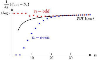
Figure 5: The entropy increment $\Delta S$ per $\Delta n=1$ is plotted as a function of the number $n$ of Planck unit arcs which tile the circular horizon. Note the number theoretical Polya bifurcation into two branches, $n$-even (blue) and $n$-odd (red) respectively, sharing a common asymptotic limit (solid curve).

It is interesting to further study the deviation from the Bekenstein-Hawking limit, in particular, for small $n$, by plotting $\Delta S_{n}=S_{n+1}-S_{n}$, the amount of entropy added by increasing the number of Planck arcs by one unit. The plot, see Fig. 5, splits into two branches, even-$n$ and odd-$n$ branches, respectively. As $n$ increases, the two branches merge to share a common asymptotic behavior Eq.(21).

VII VII. Conclusion

Identifying and counting the elusive black hole microstates is an open challenge in theoretical physics. Counterintuitively, while invoking the familiar ingredient of a fundamental Planck unit area, none of the individual units play any local role in our model. In fact, all Planck areas tiling the horizon are collectively involved in what can be described as a global realization of the ”it from bit” phrase, with the topologically distinct configurations resembling or even identified as the black hole microstates. This opens the door for graph theory and number theory to enter black hole physics under the auspices of the would be quantum gravity and/or the universal complex network Bianchi .

If Eq.(3) is not applicable to start with, our model needs to be supplemented by field theoretic ingredients or to be generalized graph theoretically. The first step would be to deal with Taub-NUT $S^{3}$ topology. Regarding black hole phase transitions (topology change or otherwise), our model cannot shed light on this aspect at this stage. Even the $n\rightarrow n-1$ quantum black hole transition is not any clearer here than that given in the standard spectral treatment of Bekenstein and Mukhanov. The fate of the ”lost” Planck horizon unit area in the process is under investigation and may hold the key to future developments.

VIII Acknowledgments

- (1) J.D. Bekenstein, Lett. Nuovo Cimento 4, 737 (1972); J.D. Bekenstein, Phys. Rev. D7, 2333 (1973); S.W. Hawking, Comm. Math. Phys. 43, 199 (1975).
- (2) A. Strominger and C. Vafa, Phys. Lett. B379, 99 (1996); S.D. Mathure, Fortschr. Phys. 53, 793 (2005); A. Sen, Gen. Rel. Grav. 46, 1711 (2014).
- (3) A. Ashtekar, J. Baez, A. Corichi and K. Krasnov Phys. Rev. Lett. 80, 904 (1998); A. Ghosh, K. Noui and A. Perez, Phys. Rev. D89, 084069 (2014); A. Perez, Rep. Prog. Phys. 80, 126901 (2017).
- (4) J. M. Maldacena, Theor. Phys. 38, 1113 (1999); S.S. Gubser, I.R. Klebanov and A.M. Polyakov, Phys. Lett. B428, 105 (1998); E. Witten, Adv. Theor. Math. Phys. 2, 253 (1998).
- (5) J. Maldacena, J. Bekenstein memorial volume, Eds. L. Brink, V. Mukhanov, E. Rabinovici and K.K. Phua (World Scientific, 2019), arXiv:1810.11492[hep-th].
- (6) J.D. Bekenstein, Phys. Rev. D9, 3292 (1974).
- (7) J.D. Bekenstein and V.F. Mukhanov, Phys. Lett. B360, 7 (1995).
- (8) S. Hod, Phys. Rev. Lett. 81, 4293 (1998); I.B. Khriplovich, Phys. Lett. B431, 19 (1998); G. Gour, Phys. Rev. D66, 104022 (2002); O. Dreyer, Phys. Rev. Lett. 90, 081301 (2003); D. Dou and R. Sorkin, Found. of Phys. 33, 279 (2003); M. Maggiore, Phys. Rev. 100, 141301 (2008); G. Dvali and C. Gomez, Fortschr. Phys. 59, 579 (2011); A. Davidson, IJMPD 23, 1450041 (2014); D. Oriti,1, D. Pranzetti and L. Sindoni, Phys. Rev. Lett. 116, 211301 (2016); V.F. Foit and M. Kleban, Class. Quant. Grav. 36, 035006 (2019).
- (9) J. Wheeler, Proc. 3rd Int. Symp. on Foundations of Quantum Mechanics” p.354 (Phys. Soc. Japan (1990), Tokyo, 1989).
- (10) G. ’t Hooft, in Salam Festschrifft, eds. A. Aly, J. Ellis and S. Randjbar Daemi (World Scientific, 1993); L. Susskind, J. Math. Phys. 36, 6377 (1995).
- (11) G. Polya, Acta Math. 68, 145 (1937); N. L. Biggs, Discrete Mathematics, (Oxford University Press, 1994).
- (12) S. W. Hawking, Commun. Math. Phys. 25, 152 (1972).
- (13) https://github.com/falk-hueffner/tinygraph.
- (14) C. McDiarmid, A. Steger, and D. J.A. Welsh, J. Combin. Theory Ser-B 93, 187 (2005).
- (15) O. Gimenez and M. Noy, J. Amer. Math. Soc. 22, 309 (2009).
- (16) M. Bodirsky, E. Fusy, M. Kang and S. Vigerske, Elect. Jour. of Combin. 14, R66 (2007).
- (17) G. Chapuy, E. Fusy, O. Gimenez, B. Mohar and M. Noy, J. Combin. Theory Ser-A 118, 748 (2011).
- (18) A. Denise, M. Vasconcellos, and D. J.A. Welsh, Congr. Numer. 113, 61 (1996).
- (19) N. Bonichon, C. Gavoille, N. Hanusse, D. Poulalhon, and G. Schaeffer, Graphs and Combin. 22,185 (2006).
- (20) W.T. Tutte, Canad. J. Math 14, 21 (1962).
- (21) J.L. Cardy, Nucl. Phys. B270, 186 (1986).
- (22) S. Carlip, Class. Quant. Grav. 17, 4175 (2000).
- (23) R.K. Kaul and P. Majumdar, Phys. Rev. Lett. 84, 5255 (2000); A. Chatterjee and P. Majumdar, Phys. Rev. Lett. 92, 141301 (2004); C. Kiefer and G. Kolland, Gen. Rel. Grav. 40, 1327 (2008).
- (24) E.R. Livine and D.R. Terno, Nucl. Phys. B741, 131 (2006); A. Corichi, J. Diaz-Polo and E. Fernandez-Borja, Phys. Rev. Lett. 98, 181301 (2007); E. Bianchi, Class. Quant. Grav. 28, 114006 (2011).
- (25) M. Banados, C. Teitelboim and J. Zanelli, Phys. Rev. Lett. 69, 1849 (1992).
- (26) http://mathworld.wolfram.com/Necklace.html
- (27) http://mathworld.wolfram.com/TotientFunction.html
- (28) G. Bianconi and A.L. Barabasi, Phys. Rev. Lett. 86, 5632 (2001).