Higher-Order Sudakov Resummation in Coupled Gauge Theories

Abstract

We consider the higher-order resummation of Sudakov double logarithms in the presence of multiple coupled gauge interactions. The associated evolution equations depend on the coupled $\beta$ functions of two (or more) coupling constants $\alpha_{a}$ and $\alpha_{b}$, as well as anomalous dimensions that have joint perturbative series in $\alpha_{a}$ and $\alpha_{b}$. We discuss possible strategies for solving the system of evolution equations that arises. As an example, we obtain the complete three-loop (NNLL) QCD$\otimes$QED Sudakov evolution factor. Our results also readily apply to the joint higher-order resummation of electroweak and QCD Sudakov logarithms.

As part of our analysis we also revisit the case of a single gauge interaction (pure QCD), and study the numerical differences and reliability of various methods for evaluating the Sudakov evolution factor at higher orders. We find that the approximations involved in deriving commonly used analytic expressions for the evolution kernel can induce noticeable numerical differences of several percent or more at low scales, exceeding the perturbative precision at N³LL and in some cases even NNLL. Therefore, one should be cautious when using approximate analytic evolution kernels for high-precision analyses.

1 Introduction

In perturbative quantum field theories it is well known that observables sensitive to physics at different scales $\mu\ll\mu_{0}$ can have their perturbative expansions in the coupling constant $\alpha$ generically enhanced by Sudakov logarithms of the form

$$\alpha(\mu)^{n}\ln^{m}\frac{\mu}{\mu_{0}}\qquad\text{with}\qquad m\leq 2n\,.$$ (1.1)

For sufficiently separated scales, the logarithms grow large enough to dominate (and eventually deteriorate) the perturbative series. The reliability and precision of theoretical predictions can therefore be improved (or restored) by a reorganization of the perturbative series into a form that keeps the highest-power logarithms to all orders in $\alpha$, a procedure called resummation. Various different formalisms have been developed to achieve the resummation, with strongly interacting processes being the most widely studied due to their dominant contribution to many key collider processes. Indeed, multiple observables have been resummed to next-to-next-to-leading logarithmic (NNLL) and even N³LL accuracy within QCD, in an effort to match the ever increasing experimental precision.

Despite their smaller couplings in the Standard Model (SM), corrections from the emission of electroweak (EW) bosons can be comparable to those of QCD calculated at NNLO (cf. $\alpha_{e}\sim\alpha_{s}^{2}$). Furthermore, the exchange of massive virtual EW bosons in high-energy processes can generate EW Sudakov logarithms of the form of eq. (1.1), which can cause sizeable EW corrections. The resummation of EW Sudakov logarithms has been studied for many years, albeit typically at lower orders than in QCD, see e.g. refs. [1, 2, 3, 4, 5, 6, 7, 8, 9, 10, 11, 12, 13, 14]. As a result, achieving sufficiently precise predictions for many collider observables requires considering them in a joint QCD$\otimes$EW environment to fully capture all relevant effects. This is of course true when considering an extremely high energy future collider [15], where EW corrections can be $\mathcal{O}(1)$, but also for measurements at the LHC reaching percent-level precision, the prime example being the high-precision measurements of $W$ and $Z$ production [16, 17, 18, 19, 20, 21]. The recent literature reflects this: The impact of EW and mixed QCD$\otimes$EW corrections on the $W$-mass measurement have received much attention (see e.g. refs. [22, 23, 24, 25] and references therein). QED corrections to the evolution of parton distribution functions (PDFs) have also been obtained, see e.g. refs. [26, 27, 28, 29, 30, 31]. The full NNLO $\mathcal{O}(\alpha_{e}\alpha_{s})$ mixed QCD$\otimes$QED corrections and $\mathcal{O}(\alpha_{e}^{2})$ QED corrections for on-shell $Z$ production were calculated recently in ref. [32] and for Higgs production in bottom-quark annihilation in ref. [33]. The one-loop QED corrections to the Sudakov resummation were included in the high-precision analysis of thrust in $e^{+}e^{-}$ collisions [34]. The resummed $p_{T}$ spectrum of $Z$-boson production including QED corrections was obtained in ref. [35], capturing the pure QED logarithmic contributions at NLL and the mixed QCD$\otimes$QED contributions at LL. Closely related, the QED corrections to the two-loop anomalous dimensions of $p_{T}$-dependent distributions were obtained in ref. [36] and of the quark form factors in ref. [33].

In this paper, we step back and reevaluate some of the technical aspects of Sudakov resummation when the interactions of two gauge symmetries $G_{a}\otimes G_{b}$ are involved, staying agnostic as to the precise resummation formalism utilized. In particular, we analyze the integrand structure of the Sudakov evolution factor

$$U(\mu_{0},\mu)=\exp\biggl{\{}\int_{\mu_{0}}^{\mu}\frac{d\mu^{\prime}}{\mu^{\prime}}\Gamma_{\mathrm{cusp}}[\alpha_{a}(\mu^{\prime}),\alpha_{b}(\mu^{\prime})]\ln\frac{Q}{\mu^{\prime}}+\gamma[\alpha_{a}(\mu^{\prime}),\alpha_{b}(\mu^{\prime})]\biggr{\}}\,.$$ (1.2)

An evolution factor of this form necessarily appears in all formulations of higher-order Sudakov resummation. It implicitly depends on the $\beta$ functions controlling the renormalization group evolution (RGE) of both gauge coupling constants $\alpha_{a}(\mu)$ and $\alpha_{b}(\mu)$, which in general are a coupled system of differential equations, as well as anomalous dimensions ($\Gamma_{\mathrm{cusp}},\gamma$) whose perturbative expansions are themselves joint series in $\alpha_{a,b}$. We attempt to be as generic as possible in our discussion and therefore do not immediately specify $G_{a,b}$. To draw some phenomenological conclusions we will eventually consider the example of QCD$\otimes$QED, i.e. $G_{a}\equiv SU(3)_{c}$ and $G_{b}\equiv U(1)_{\rm em}$, for which we obtain the complete three-loop (NNLL) Sudakov evolution factor.

Interestingly, we also find that the approximations made in obtaining closed-form analytic expressions for eq. (1.2) that are commonly used in the literature can lead to nonnegligible numerical differences. When evolving to low scales, where the resummation becomes most important, the resulting effects can reach several percent or more. In other words, the use of different strategies for evaluating eq. (1.2) can be a source of nontrivial systematic differences between different resummation implementations that can potentially exceed the perturbative precision one is aiming for. As one manifestation, we find nontrivial violations of the consistency of the evolution, which we probe by testing the closure condition

$$U(\mu,\mu_{0})\,U(\mu_{0},\mu)\overset{!}{=}1\,.$$ (1.3)

Since these issues already appear for a single gauge interaction we devote a substantial fraction of our paper to exploring them in this simpler case, using pure QCD as test case. We consider various combinations of numerical and approximate analytic treatments of the Sudakov factor and study their accuracy. Ultimately, we are forced to conclude that the commonly used approximate analytic expressions for eq. (1.2) are not sufficiently reliable when aiming for percent-level precision. We find that a seminumerical approach, where the $\mu$-integration in the exponent of eq. (1.2) is carried out numerically while using an approximate analytic solution for the running of the coupling, provides a good compromise, which also straightforwardly generalizes to multiple gauge interactions.

The structure of the paper is as follows. In section 2, we discuss the coupled $\beta$ functions for $\alpha_{a,b}$. We first review the standard approximate analytic solutions for $\alpha$ in the one-dimensional case, and then derive corresponding approximate analytic solutions for the coupled system up to three-loop (NNLO) running. In section 3, we move to analyzing the Sudakov evolution kernels for the one-dimensional case, discussing several methods for evaluating it and studying their numerical performance up to N³LL. In section 4 we then apply the lessons learned to the case of two coupled gauge interactions. We conclude in section 5. In appendix A, we provide the perturbative ingredients utilized in our numerical comparisons, including the complete set of three-loop QCD$\otimes$QED coefficients. In appendix B, we discuss the extraction of the complete three-loop mixed QCD$\otimes$QED $\beta$-function coefficients.

2 Iterative solutions to $\beta$-function RGEs

Before discussing the evaluation of the Sudakov evolution kernel, it will be important to analyze one of its key ingredients, namely the solution of the $\beta$-function RGE of the coupling constant. In subsection 2.1, we review the well-known case of a single gauge theory, with particular attention given to the numerical accuracy of different approximate analytic RGE solutions. In subsection 2.2 we then discuss the solution of the coupled RGE system for the coupling constants of two gauge theories.

2.1 Single gauge theory

We start from the well-known $\beta$-function RGE for the coupling constant $\alpha(\mu)$ of a generic gauge theory,

$$\frac{\mathrm{d}\alpha(\mu)}{\mathrm{d}\ln\mu}\equiv\beta[\alpha(\mu)] =-2\alpha(\mu)\sum_{n=0}^{\infty}\epsilon^{n}\beta_{n}\Bigl{[}\frac{\alpha(\mu)}{4\pi}\Bigr{]}^{n+1}$$

$$=-2\beta_{0}\,\frac{\alpha(\mu)^{2}}{4\pi}\,\biggl{[}1+\epsilon\,\frac{\alpha(\mu)}{4\pi}\,b_{1}+\epsilon^{2}\,\frac{\alpha(\mu)^{2}}{(4\pi)^{2}}\,b_{2}+\mathcal{O}(\epsilon^{3})\biggr{]}\,.$$ (2.1)

Here, $\mu$ is the renormalization scale, and we introduced a formal expansion parameter $\epsilon\equiv 1$, which we use to keep track of the evolution order. The perturbative coefficients $b_{n}$ in the second line are defined by the ratio

$$b_{n}=\frac{\beta_{n}}{\beta_{0}}\,.$$ (2.2)

We take the viewpoint that eq. (2.1) defines the running order of the RGE. That is, keeping the terms up to $\mathcal{O}(\epsilon^{k})$ in eq. (2.1) defines the N^kLO or ($k+1$)-loop running of $\alpha(\mu)$. At leading order, $\mathcal{O}(\epsilon^{0})$, eq. (2.1) has the well-known exact analytic solution,

$$\alpha(\mu)=\frac{\alpha(\mu_{0})}{X}\,,\qquad X\equiv X(\mu_{0},\mu)=1+\frac{\alpha(\mu_{0})}{2\pi}\,\beta_{0}\,\ln\frac{\mu}{\mu_{0}}\,,$$ (2.3)

where $\alpha(\mu_{0})$ is a boundary condition for the coupling constant.

As is well known, eq. (2.1) does not admit an exact analytic solution at NLO and beyond. While the exact solution can be easily obtained numerically using standard numerical differential-equation solvers, in practice it is often more convenient to have an approximate analytic solution that can be evaluated much faster than the numerical solution, which becomes important when the scale $\mu$ is not fixed but dynamical. This is precisely the case for the Sudakov evolution kernel, for which we will need to integrate $\alpha(\mu)$ over $\mu$.

In what follows, we review an iterative method to obtain an approximate analytic solution for eq. (2.1). At NLO, $\mathcal{O}(\epsilon)$, the $\beta$-function RGE reads

$$\frac{\mathrm{d}\alpha(\mu)}{\mathrm{d}\ln\mu} =-2\beta_{0}\frac{\alpha(\mu)^{2}}{4\pi}\biggl{[}1+\epsilon\,\frac{\alpha(\mu)}{4\pi}\,b_{1}\biggr{]}$$

$$=-2\beta_{0}\frac{\alpha(\mu)^{2}}{4\pi}\biggl{[}1+\epsilon\,\frac{\alpha(\mu_{0})}{4\pi}\,\frac{b_{1}}{X(\mu_{0},\mu)}+\mathcal{O}(\epsilon^{2})\biggr{]}\,.$$ (2.4)

In the second line we substituted the LO solution in eq. (2.3) for the $\mu$ dependence of $\alpha(\mu)$ in the $\mathcal{O}(\epsilon)$ term. This induces an $\mathcal{O}(\epsilon^{2})$ error, since the difference between the LO and NLO $\mu$ dependence will itself be of $\mathcal{O}(\epsilon)$. Since the $\mu$ dependence in the term in square brackets is now explicit, it can be easily integrated, yielding the NLO solution

$$\frac{1}{\alpha(\mu)} =\frac{X}{\alpha(\mu_{0})}+\epsilon\,\frac{b_{1}}{4\pi}\,\ln X\,,$$

$$\Rightarrow\qquad\alpha(\mu) =\alpha(\mu_{0})\biggl{[}X+\epsilon\,\frac{\alpha(\mu_{0})}{4\pi}\,b_{1}\ln X\biggr{]}^{-1}\,.$$ (2.5)

We refer to this (and its higher-order analogues) as the “iterative” solution for $\alpha(\mu)$. We can also expand the inverse in eq. (2.1) in $\epsilon$ to obtain

$$\alpha(\mu) =\frac{\alpha(\mu_{0})}{X}\biggl{[}1-\epsilon\,\frac{\alpha(\mu_{0})}{4\pi}\,b_{1}\,\frac{\ln X}{X}+\mathcal{O}(\epsilon^{2})\biggr{]}\,.$$ (2.6)

We will refer to eq. (2.6) (and its higher-order analogues) as the “expanded” solution.

One might wonder whether the iterative or expanded solution provides a better approximation to the exact solution, and to this end it is instructive to see to what extent they satisfy the original $\beta$-function RGE. For the iterative solution in eq. (2.1), it is trivial to verify that upon differentiation with respect to $\ln\mu$ it reproduces the RGE as given in the second line of eq. (2.1). On the other hand, taking the $\ln\mu$ derivative of the expanded NLO solution in eq. (2.6) yields

$$\frac{\mathrm{d}\alpha(\mu)}{\mathrm{d}\ln\mu} =-2\beta_{0}\,\frac{\alpha(\mu_{0})^{2}}{4\pi}\,\frac{1}{X^{2}}\biggl{[}1+\epsilon\,\frac{\alpha(\mu_{0})}{4\pi}\,b_{1}\,\frac{1-2\ln X}{X}\biggr{]}$$

$$=-2\beta_{0}\,\frac{\alpha(\mu_{0})^{2}}{4\pi}\,\frac{1}{X^{2}}\biggl{\{}\biggl{[}1-2\epsilon\,\frac{\alpha(\mu_{0})}{4\pi}\,b_{1}\,\frac{\ln X}{X}\biggl{]}+\epsilon\,\frac{\alpha(\mu_{0})}{4\pi}\,\frac{b_{1}}{X}\biggr{\}}\,.$$ (2.7)

Comparing this with eqs. (2.1) and (2.6), we see that the term in square brackets corresponds to expanding the overall $\alpha(\mu)^{2}$ in the $\beta$ function to $\mathcal{O}(\epsilon)$. This clearly amounts to a further approximation, so we can expect the expanded solution in general to provide a worse approximation, which is indeed what we will find numerically below.

The iterative solution at NNLO, $\mathcal{O}(\epsilon^{2})$, follows analogously. Starting from the exact NNLO RGE, we substitute the (expanded) NLO and LO solutions, eqs. (2.6) and (2.3), in the $\mathcal{O}(\epsilon)$ and $\mathcal{O}(\epsilon^{2})$ terms, keeping all terms up to $\mathcal{O}(\epsilon^{2})$ as well as the overall $\alpha(\mu)^{2}$,

$$\frac{\mathrm{d}\alpha(\mu)}{\mathrm{d}\ln\mu} =-2\beta_{0}\frac{\alpha(\mu)^{2}}{4\pi}\biggl{[}1+\epsilon\,\frac{\alpha(\mu)}{4\pi}\,b_{1}+\epsilon^{2}\frac{\alpha(\mu)^{2}}{(4\pi)^{2}}\,b_{2}\biggr{]}$$

$$=-2\beta_{0}\frac{\alpha(\mu)^{2}}{4\pi}\biggl{[}1+\epsilon\,\frac{\alpha(\mu_{0})}{4\pi}\,\frac{b_{1}}{X}+\epsilon^{2}\,\frac{\alpha(\mu_{0})^{2}}{(4\pi)^{2}}\frac{b_{2}-b_{1}^{2}\,\ln X}{X^{2}}+\mathcal{O}(\epsilon^{3})\biggr{]}\,.$$ (2.8)

The $\mu$-dependence in the square brackets on the second line, encoded in $X\equiv X(\mu_{0},\mu)$, is again simple enough to be integrated analytically. This yields the NNLO iterative solution

$$\alpha(\mu) =\alpha(\mu_{0})\biggl{\{}X+\epsilon\,\frac{\alpha(\mu_{0})}{4\pi}\,b_{1}\ln X+\epsilon^{2}\,\frac{\alpha(\mu_{0})^{2}}{(4\pi)^{2}}\biggl{(}b_{2}\,\frac{X-1}{X}+b_{1}^{2}\,\frac{1-X+\ln X}{X}\biggr{)}\biggr{\}}^{-1}\,.$$ (2.9)

Expanding the inverse in eq. (2.9) in $\epsilon$, we obtain the expanded NNLO solution,

$$\alpha(\mu) =\frac{\alpha(\mu_{0})}{X}\biggl{\{}1-\epsilon\,\frac{\alpha(\mu_{0})}{4\pi}\,b_{1}\,\frac{\ln X}{X}$$

$$\quad+\epsilon^{2}\,\frac{\alpha(\mu_{0})^{2}}{(4\pi)^{2}}\,\frac{1}{X^{2}}\Bigl{[}b_{2}(1-X)+b_{1}^{2}\,(\ln^{2}X-\ln X-1+X)\Bigr{]}+\mathcal{O}(\epsilon^{3})\biggr{\}}\,.$$ (2.10)

It is straightforward to extend the iterative solution to higher orders. To obtain the N^kLO solution, one simply inserts the N^k-1LO solution for $\alpha(\mu)$ into the N^kLO $\beta$ function and expands it to $\mathcal{O}(\epsilon^{k})$, while keeping the overall $\alpha(\mu)^{2}$ exact. The N³LO solution is given in appendix A.1.

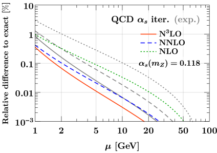
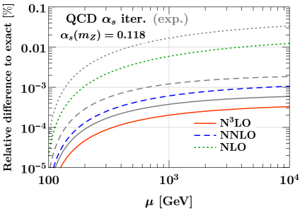
Figure -899: Relative deviation of the iterative (colored) and expanded solutions (gray) from the exact solution for the running of $\alpha_{s}(\mu)$ at NLO (dotted), NNLO (dashed), and N³LO (solid).

To illustrate the numerical precision of the approximate analytic solutions, we take the QCD coupling constant $\alpha_{s}(\mu)$ as an example, using $\alpha_{s}(m_{Z})=0.118$ as our boundary condition. As we are primarily interested in the numerical precision of the solution, we always use $n_{f}=5$ massless flavors and do not consider any flavor thresholds. The difference of the iterative and expanded solutions to the exact numerical solution, which we refer to as the approximation error, is shown in figure -899 for different running orders.

The approximation error decreases as the order increases, as expected. The approximation error is largest for running from $m_{Z}$ down to lower scales, since here the running increases the coupling. The iterative solution still provides an excellent approximation, with the error at NNLO and beyond reaching at most 0.1% when running down to $\mu=2\,\mathrm{GeV}$, and at most 0.3% at $\mu=1\,\mathrm{GeV}$. For running above $m_{Z}$, the approximation error is much smaller due to asymptotic freedom. Beyond the highest scale shown, $\mu=10^{4}\,\mathrm{GeV}$, the error stops growing and at some point starts decreasing again. We also observe that the approximation error for the expanded solution (gray lines) is always 2-3 times larger than for the iterative solution.

2.2 Two coupled gauge theories

We now consider the case of two gauge theories. Their $\beta$ functions become coupled as soon as there are matter fields that are charged under both gauge interactions, since loops of matter particles can exchange the gauge bosons from both theories. The example we will eventually consider is the mixed QCD$\otimes$QED running. For now, we keep the discussion general and consider the following set of coupled $\beta$-function RGEs for two gauge couplings $\alpha_{a}(\mu)$ and $\alpha_{b}(\mu)$,

$$\frac{\mathrm{d}\alpha_{a}(\mu)}{\mathrm{d}\ln\mu} \equiv\beta^{a}[\alpha_{a}(\mu),\alpha_{b}(\mu)]=-2\alpha_{a}(\mu)\sum_{n,k=0}^{\infty}\epsilon^{n}_{a}\epsilon_{b}^{k}\,\beta^{a}_{nk}\,\Bigl{[}\frac{\alpha_{a}(\mu)}{4\pi}\Bigr{]}^{n+1}\Bigl{[}\frac{\alpha_{b}(\mu)}{4\pi}\Bigr{]}^{k}\,,$$

$$\frac{\mathrm{d}\alpha_{b}(\mu)}{\mathrm{d}\ln\mu} \equiv\beta^{b}[\alpha_{b}(\mu),\alpha_{a}(\mu)]=-2\alpha_{b}(\mu)\sum_{n,k=0}^{\infty}\epsilon^{n}_{b}\epsilon_{a}^{k}\,\beta^{b}_{nk}\,\Bigl{[}\frac{\alpha_{b}(\mu)}{4\pi}\Bigr{]}^{n+1}\Bigl{[}\frac{\alpha_{a}(\mu)}{4\pi}\Bigr{]}^{k}\,.$$ (2.11)

We have again introduced formal expansion parameters $\epsilon_{a,b}\equiv 1$ to easily keep track of the evolution order. For future convenience, we also define the rescaled coefficients

$$b^{a}_{nk}=\frac{\beta^{a}_{nk}}{\beta^{a}_{00}}\,,\qquad b^{b}_{nk}=\frac{\beta^{b}_{nk}}{\beta^{b}_{00}}\,,\qquad\text{and}\qquad b_{0}^{a}=\frac{\beta_{00}^{a}}{\beta^{b}_{00}}\,,\qquad b_{0}^{b}=\frac{\beta_{00}^{b}}{\beta^{a}_{00}}\,.$$ (2.12)

Note that by definition $\beta^{x}_{n0}\equiv\beta_{n}$ and $b^{x}_{n0}\equiv b_{n}$ are the coefficients of the individual gauge theories in the absence of the second.

As before, the order in $\epsilon_{a,b}$ to which eq. (2.2) is expanded is what defines the running order of the couplings. Generically, we consider $\epsilon_{a,b}$ on equal footing and define the NⁿLO evolution by including in eq. (2.2) all terms of $\mathcal{O}(\epsilon_{a}^{k}\epsilon_{b}^{n-k})$ with $0\leq k\leq n$. Note that this also makes it easy to have well-defined mixed orders, e.g., when there is a hierarchy between the two couplings, as is the case for QCD and QED. For this purpose, one can simply specify the explicit combinations of powers of $\epsilon_{a}$ and $\epsilon_{b}$ that are included in eq. (2.2).

As in the single gauge scenario, an exact solution to the coupled system of differential equations can be obtained straightforwardly at any given order by solving it numerically. Our goal is to derive an approximate analytic solution for the coupled $\beta$-function RGE system by extending the iterative method in subsection 2.1. The key property of eq. (2.2) that allows us to do so is that, at leading order, $\mathcal{O}(\epsilon_{a}^{0},\epsilon_{b}^{0})$, the RGE system decouples, yielding exact LO solutions:

$$\alpha_{a}(\mu) =\frac{\alpha_{a}(\mu_{0})}{X_{a}}\,,\qquad X_{a} \equiv X_{a}(\mu_{0},\mu)=1+\frac{\alpha_{a}(\mu_{0})}{2\pi}\,\beta^{a}_{00}\,\ln\frac{\mu}{\mu_{0}}\,,$$

$$\alpha_{b}(\mu) =\frac{\alpha_{b}(\mu_{0})}{X_{b}}\,,\qquad X_{b} \equiv X_{b}(\mu_{0},\mu)=1+\frac{\alpha_{b}(\mu_{0})}{2\pi}\,\beta^{b}_{00}\,\ln\frac{\mu}{\mu_{0}}\,.$$ (2.13)

To obtain an approximate NLO solution, it then suffices to substitute the above LO solutions into the $\mathcal{O}(\epsilon_{a})$ and $\mathcal{O}(\epsilon_{b})$ terms of the NLO RGE system, which induces $\mathcal{O}(\epsilon_{a}^{2},\epsilon_{a}\epsilon_{b},\epsilon_{b}^{2})$ errors,

$$\frac{\mathrm{d}\alpha_{a}(\mu)}{\mathrm{d}\ln\mu} =-2\beta_{00}^{a}\frac{\alpha_{a}(\mu)^{2}}{4\pi}\biggl{[}1+\epsilon_{a}\,\frac{\alpha_{a}(\mu)}{4\pi}\,b^{a}_{10}+\epsilon_{b}\,\frac{\alpha_{b}(\mu)}{4\pi}\,b^{a}_{01}\biggr{]}$$ (2.14)

$$=-2\beta_{00}^{a}\frac{\alpha_{a}(\mu)^{2}}{4\pi}\biggl{[}1+\epsilon_{a}\,\frac{\alpha_{a}(\mu_{0})}{4\pi}\,\frac{b^{a}_{10}}{X_{a}(\mu_{0},\mu)}+\epsilon_{b}\,\frac{\alpha_{b}(\mu_{0})}{4\pi}\,\frac{b^{a}_{01}}{X_{b}(\mu_{0},\mu)}+\mathcal{O}(\epsilon_{a}^{2},\epsilon_{a}\epsilon_{b},\epsilon_{b}^{2})\biggr{]}\,.$$

The terms in square brackets can now be explicitly integrated over $\ln\mu$ to obtain the iterative NLO solution

$$\alpha_{a}(\mu)=\alpha_{a}(\mu_{0})\biggl{[}X_{a}+\frac{\alpha_{a}(\mu_{0})}{4\pi}\Bigl{(}\epsilon_{a}\,b_{10}^{a}\,\ln X_{a}+\epsilon_{b}\,b^{a}_{0}\,b_{01}^{a}\,\ln X_{b}\Bigr{)}\biggr{]}^{-1}\,.$$ (2.15)

The solution for $\alpha_{b}(\mu)$ is given by replacing $a\leftrightarrow b$ everywhere.

Note that in eq. (2.15) the utility of the $\epsilon_{a,b}$ counting parameters becomes evident. Naively, one might have expected that the $\mathcal{O}(\epsilon_{a})$ and $\mathcal{O}(\epsilon_{b})$ terms will be proportional to $\alpha_{a}(\mu_{0})$ and $\alpha_{b}(\mu_{0})$ respectively, which however is not the case, as both are proportional to $\alpha_{a}(\mu_{0})$. Instead, the $\epsilon_{a,b}$ actually keep track of the fact that the $\ln X_{a,b}$ factors respectively resum a series of $\alpha_{a,b}^{n}\ln^{n}(\mu/\mu_{0})$ terms.

The iterative NNLO solution is obtained by substituting the NLO solutions into the $\beta$-function RGE system and expanding it to $\mathcal{O}(\epsilon_{a}^{2},\epsilon_{a}\epsilon_{b},\epsilon_{b}^{2})$, while keeping the overall $\alpha_{a,b}(\mu)^{2}$ exact. We find

$$\frac{\alpha_{a}(\mu_{0})}{\alpha_{a}(\mu)} =X_{a}+\epsilon_{a}\,\frac{\alpha_{a}(\mu_{0})}{4\pi}\,b_{10}^{a}\ln X_{a}+\epsilon_{a}^{2}\,\frac{\alpha_{a}(\mu_{0})^{2}}{(4\pi)^{2}}\biggl{(}b_{20}^{a}\,\frac{X_{a}-1}{X_{a}}+(b_{10}^{a})^{2}\frac{1-X_{a}+\ln X_{a}}{X_{a}}\biggr{)}$$

$$\quad+\epsilon_{b}\,\frac{\alpha_{a}(\mu_{0})}{4\pi}\,b^{a}_{0}\,b_{01}^{a}\ln X_{b}+\epsilon_{b}^{2}\,\frac{\alpha_{a}(\mu_{0})\alpha_{b}(\mu_{0})}{(4\pi)^{2}}b^{a}_{0}\biggl{(}b_{02}^{a}\,\frac{X_{b}-1}{X_{b}}+b_{01}^{a}b_{10}^{b}\,\frac{1-X_{b}+\ln X_{b}}{X_{b}}\biggr{)}$$

$$\quad+\epsilon_{a}\epsilon_{b}\,\frac{\alpha_{a}(\mu_{0})}{b_{0}^{a}\,\alpha_{a}(\mu_{0})-\alpha_{b}(\mu_{0})}\biggl{[}\frac{\alpha_{a}^{2}(\mu_{0})}{(4\pi)^{2}}(b^{a}_{0})^{2}b_{10}^{a}b_{01}^{a}\biggl{(}\frac{X_{b}}{X_{a}}\ln X_{b}-\frac{1-X_{b}}{1-X_{a}}\ln X_{a}\biggr{)}$$

$$\qquad-\frac{\alpha_{b}^{2}(\mu_{0})}{(4\pi)^{2}}\,b_{01}^{a}b_{01}^{b}\biggl{(}\frac{X_{a}}{X_{b}}\ln X_{a}-\frac{1-X_{a}}{1-X_{b}}\ln X_{b}\biggr{)}+\frac{\alpha_{a}(\mu_{0})\alpha_{b}(\mu_{0})}{(4\pi)^{2}}b^{a}_{0}\,b_{11}^{a}\ln\frac{X_{a}}{X_{b}}\biggr{]}\,.$$ (2.16)

As before, the solution for $\alpha_{b}(\mu)$ is obtained by replacing $a\leftrightarrow b$. The terms in the first line correspond to the NNLO solution of $\alpha_{a}$ in the absence of $\alpha_{b}$, while the remaining ones are the mixing contributions involving at least one power of $\epsilon_{b}$. The corresponding expanded solution is obtained by inverting eq. (2.2) and expanding it in $\epsilon_{i}$. Note that when doing so, it becomes essential to expand in terms of $\epsilon_{i}$ and not $\alpha_{i}(\mu_{0})$. The necessity of using $\epsilon_{i}$ as expansion parameter is also evident in the mixed $\mathcal{O}(\epsilon_{a}\epsilon_{b})$ term in square brackets, which involves a nontrivial rational function of both couplings. The above iterative NNLO solution will be a key ingredient in the seminumerical evaluation of the Sudakov evolution factor in section 4.

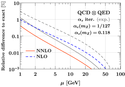
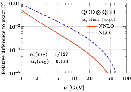
Figure -898: Relative deviation from the exact solution for the running of the QCD (left) and QED (right) coupling constants in QCD$\otimes$QED for the iterative (colored) and expanded (gray) solutions.

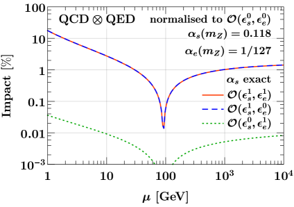
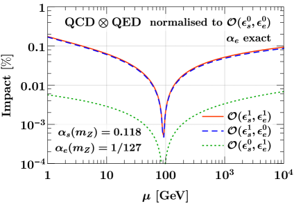
Figure -897: Impact of different higher-order terms on the running of the QCD (left) and QED (right) couplings. Shown are the relative differences to the LO running $\sim\mathcal{O}(\epsilon_{s}^{0},\epsilon_{e}^{0})$.

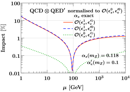
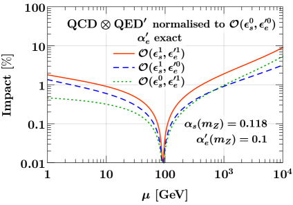
Figure -896: Same as figure -897 but for QCD$\otimes$QED^′, where QED^′ is a toy theory with a modified boundary condition of $\alpha_{e}^{\prime}(m_{Z})=0.1$.

To illustrate the approximation error for the two analytic solutions, we consider the case of QCD$\otimes$QED. The relevant coefficients for the coupled $\beta$-function RGE to NNLO are given in appendices A.2 and A.3. Curiously, we were not able to find explicit expressions in the literature for the mixed three-loop QED coefficient $\beta_{11}^{e}$. We therefore performed an explicit extraction of all mixed three-loop coefficients from the general results for a generic product group given in ref. [37], as discussed in more detail in appendix B.

For the numerical results, we use $\alpha_{s}(m_{Z})=0.118$ and $\alpha_{e}(m_{Z})=1/127$ as boundary conditions, $n_{f}=5$ for the number of active quark flavors, and $n_{\ell}=3$ for the number of active charged leptons. As before we do not consider any flavor thresholds.

The approximation error of the iterative (expanded) solution relative to the exact numerical solution is shown in figure -898 by the colored (gray) lines at NLO (dashed) and NNLO (solid). For the strong coupling constant (left panel), the approximation error for the iterative solution does not exceed 1%, and it is again 2-3 times larger for the expanded solution. For the QED coupling constant (right panel), the approximation error is much smaller owing to the fact that $\alpha_{e}$ is much smaller, and therefore both the iterative and expanded solutions yield equally good approximations.

It is interesting to see the individual effects of various terms in the coupled $\beta$ function. In figures -897 and -896 we show them for the case of QCD$\otimes$QED as well as for a toy QCD$\otimes$QED^′ for which we set the boundary condition to $\alpha_{e}^{\prime}(m_{Z})=1/10$. In figure -897, as expected, the QED corrections $\sim\mathcal{O}(\epsilon^{0}_{s},\epsilon^{1}_{e})$ have almost negligible effect on $\alpha_{s}$, with only the higher order QCD corrections $\sim\mathcal{O}(\epsilon_{s}^{1},\epsilon_{e}^{0})$ being relevant. This is also the case for the QED coupling constant, whose evolution is almost entirely dictated by the QCD corrections. But this is not the case for the toy QCD$\otimes$QED^′ scenario shown in figure -896. The fact that the QCD coupling constant is still almost unaffected by the QED^′ corrections is somewhat accidental and due to the fact that the $\beta$-function coefficients $\beta^{s}_{10}$ and $\beta^{s}_{01}$ differ numerically by an order of magnitude. On the other hand, the QED^′ coupling constant now has comparable higher-order QCD and QED^′ corrections since here both $\beta$-function coefficients are of similar numerical size.

3 Sudakov evolution kernels with a single gauge interaction

In this section, we examine different strategies for evaluating the Sudakov evolution kernel for the case of a single gauge interaction, with particular emphasis on their numerical accuracy and reliability. This will then serve as a guide when considering the two-dimensional case in section 4.

In subsection 3.1, we start with a general discussion and give an overview of the different methods we will study for evaluating the Sudakov evolution factor, which are then elaborated on in subsection 3.2 to subsection 3.5. We then provide a detailed numerical comparison in subsection 3.6.

3.1 General overview

One way to systematically resum Sudakov logarithms is based on factorizing the perturbative series. The relevant factorization can be derived diagrammatically or using effective field theories (EFTs). All ingredients of the factorized cross section obey (renormalization group) evolution equations of the form

$$\frac{\mathrm{d}F(\mu)}{\mathrm{d}\ln\mu}=\gamma_{F}(\mu)\otimes F(\mu)\,,$$ (3.1)

where $\gamma_{F}(\mu)$ is the anomalous dimension, and the function $F(\mu)$ is any one of the factorized ingredients. The Sudakov resummation is then performed by solving the resulting coupled system of RGE equations.

In general, $\gamma_{F}(\mu)$ and $F(\mu)$ both depend on an additional external kinematic quantity (which appears as part of the argument of the Sudakov logarithms in the cross section). The $\otimes$ denotes the fact that $\gamma_{F}$ and $F$ are not necessarily multiplied but could be convolved in said kinematic variable. It is worth nothing that the convolution structure can play a significant role in the solution of eq. (3.1) (for a recent detailed discussion see e.g. ref. [38]). However, it does not play any role for the purpose of our discussion, so we consider only the simplest multiplicative case. In case of a convolution, one can always transform to a suitable conjugate space (e.g. Fourier or Laplace space), where the convolution turns into a simple product. The Sudakov evolution factor in that conjugate space then has the same general form we discuss here and all our conclusions apply equally.

The all-order expansion of the anomalous dimension is given by

$$\gamma_{F}(\mu)=\frac{1}{\epsilon}\,\Gamma_{\mathrm{cusp}}[\alpha(\mu)]\ln\frac{Q}{\mu}+\gamma[\alpha(\mu)]\,,$$ (3.2)

where $Q$ denotes the above-mentioned kinematic quantity, $\Gamma_{\mathrm{cusp}}$ is (proportional to) the cusp anomalous dimension, and $\gamma$ is the noncusp anomalous dimension. They obey the perturbative expansions

$$\Gamma_{\mathrm{cusp}}(\alpha)=\sum_{n=0}^{\infty}\epsilon^{n+1}\,\Gamma_{n}\,\Bigl{(}\frac{\alpha}{4\pi}\Bigr{)}^{n+1}\,,\qquad\gamma(\alpha)=\sum_{n=0}^{\infty}\epsilon^{n+1}\,\gamma_{n}\,\Bigl{(}\frac{\alpha}{4\pi}\Bigr{)}^{n+1}\,.$$ (3.3)

We have again introduced the formal expansion parameter $\epsilon\equiv 1$, which we will use to define the resummation order. Since the $\mu$ dependence of $\gamma_{F}(\mu)$ primarily enters via the coupling constant’s $\mu$ dependence, the $\beta$ RGE for $\alpha(\mu)$ in eq. (2.1) is an integral part of the full RGE system to be solved. In particular, the $\epsilon$ parameter in eqs. (3.2) and (3.3) is the same that appears in eq. (2.1).

As for the case of the coupling constant before, the truncation of eq. (3.2) together with eq. (2.1) to a certain order in $\epsilon$ fundamentally defines the resummation order. That is, keeping terms up to $\mathcal{O}(\epsilon^{k})$ defines the Sudakov evolution at N^kLL order. The explicit $1/\epsilon$ factor for the cusp term accounts for the fact that it comes with an additional explicit logarithm relative to the noncusp term. As a result, the noncusp term always enters at one lower order in perturbation theory than the cusp term. And since the $\beta$ function in eq. (2.1) starts at $\mathcal{O}(\epsilon^{0})$, it enters at the same loop order as the cusp anomalous dimension. So as usual, at N^kLL order, we require the $k+1$-loop cusp and beta function coefficients and the $k$-loop noncusp coefficients.

Solving the RGE in eq. (3.1), one finds

$$F(\mu)=F(\mu_{0})U(\mu_{0},\mu)\,,$$ (3.4)

where $U(\mu_{0},\mu)$ is the Sudakov evolution factor given by

$$U(\mu_{0},\mu)=\exp\biggl{\{}\int_{\mu_{0}}^{\mu}\frac{\mathrm{d}\mu^{\prime}}{\mu^{\prime}}\gamma_{F}(\mu^{\prime})\biggr{\}}=\exp\biggl{\{}\int_{\mu_{0}}^{\mu}\frac{\mathrm{d}\mu^{\prime}}{\mu^{\prime}}\,\frac{1}{\epsilon}\,\Gamma_{\mathrm{cusp}}[\alpha(\mu^{\prime})]\ln\frac{Q}{\mu^{\prime}}+\gamma[\alpha(\mu^{\prime})]\biggr{\}}\,.$$ (3.5)

It resums the Sudakov logarithms appearing in the perturbative series of $F(\mu)/F(\mu_{0})$. One can easily check that counting powers of $\epsilon$ in the anomalous dimension is equivalent to counting powers of logarithms in the Sudakov exponent, simply because the entire structure of $U(\mu_{0},\mu)$ is fully encoded by the anomalous dimension. In the final resummed cross section, where $F(\mu)$ is combined with other ingredients, $U(\mu_{0},\mu)$ eventually appears with both scales $\mu$ and $\mu_{0}$ corresponding to two different kinematic quantities such that $U(\mu_{0},\mu)$ resums (part of) the Sudakov logarithms of the ratio of these quantities.

We stress that while we obtained eq. (3.5) starting from the RGE in eq. (3.1), a Sudakov evolution factor of the same structure (necessarily) appears in all the various approaches for performing Sudakov resummation that exist in the literature. This includes EFT-based and non-EFT-based approaches, and both analytic as well as numerical Monte-Carlo techniques such as parton showers.

On the other hand, different implementations tend to follow different strategies for evaluating the integral in the Sudakov exponent. In the following sections we investigate several methods for doing so, paying close attention to where additional assumptions and/or approximations are made. As we will see, additional approximations that may appear mathematically justified can still conspire to yield results for eq. (3.5) that exhibit nontrivial numerical differences. We investigate the following methods in the sections that follow:

• Numerical: In this method, both the $\beta$-function RGE eq. (2.1) and the evolution kernel eq. (3.5) are evaluated fully numerically (with sufficiently high numerical precision that numerical integration errors are negligible). This provides the exact solution of the complete Sudakov RGE system at a given resummation order as defined above, and we will use it as the benchmark to compare the other methods against. As this method can be computationally expensive, it is often not very suitable for practical purposes.

• Seminumerical: One option to speed up the fully numerically method is to employ an approximate analytic solution to the $\beta$-function RGE, but to perform the kernel integration numerically. In other words, we numerically integrate eq. (3.5) but with the iterative analytic solution for $\alpha(\mu)$ used in the perturbative expansion of the anomalous dimensions. This is described along with the fully numerical method in subsection 3.2.

• Unexpanded analytic: Approximate but fully analytic, closed-form expressions for eq. (3.5) can be obtained. One way to achieve this is to exploit the $\beta$ function to turn the $\mu$ integration into an integration over $\alpha$, which can be performed analytically after some expansion in $\epsilon$. This is combined with the analytic iterative solution for $\alpha_{s}(\mu)$ as input. We give details of the derivation and the resulting forms explicitly in subsection 3.3.

• Expanded analytic: Another way to obtain an approximate closed-form result for eq. (3.5) is to insert the analytic solution for $\alpha(\mu)$ in eq. (2.1) in the perturbative expansions of $\Gamma(\alpha)$ and $\gamma(\alpha)$ and fully expanding the integrand in $\epsilon$. The integration can then be performed directly in terms of $\mu$. This method is described in more detail in subsection 3.4.

• Reexpanded analytic: Finally, to connect to some of the available literature, we elaborate another analytic approach where, upon achieving the expanded analytic evolution kernels, one further expands $\alpha(\mu_{0})$ in terms of $\alpha(\mu_{R})$ at a different reference scale $\mu_{R}$, assuming that $\mu_{0}\sim\mu_{R}$, i.e., that there is no hierarchy between them. This method is discussed in more detail in subsection 3.5.

Given these five methods of integration, we will probe their reliability in two different ways in subsection 3.6: closure tests and approximation errors. The latter simply tests the absolute difference between any one method and the numerically exact method described above. The closure test provides a test of the mathematical consistency of the evolution factor. That is, it should satisfy the renormalization group property

$$U(\mu_{0},\mu_{1})\,U(\mu_{1},\mu_{2})=U(\mu_{0},\mu_{2})\,,$$ (3.6)

which is obvious from its definition in eq. (3.5). A simple way to test that eq. (3.6) is satisfied is to consider the special case of $\mu_{2}=\mu_{0}$, which yields

$$U(\mu_{0},\mu)\,U(\mu,\mu_{0})=1\,,$$ (3.7)

and simply expresses the fact that the RG evolution should close on itself. Since the intermediate scale here is completely arbitrary, this property should be satisfied exactly at any given order. However, deviations from unity can arise due to simplifying assumptions or approximations made in evaluating the integral in the exponent.

3.2 Numerical and seminumerical methods

The most accurate method of integration is to perform the integration fully numerically. The error introduced by the numerical integration routine can be made arbitrarily small at the expense of computing time. We always use a sufficiently high integration precision that the numerical integration error is completely negligible.

Our strategy in the numerical and seminumerical approaches is summarized schematically as

$$U(\mu_{0},\mu)=\exp\biggl{\{}\underbrace{\int_{\mu_{0}}^{\mu}\frac{\mathrm{d}\mu^{\prime}}{\mu^{\prime}}}_{\text{numerical}}\sum_{n=0}^{\infty}\biggl{[}\epsilon^{n}\Gamma_{n}\!\!\!\overbrace{\Bigl{(}\frac{\alpha(\mu^{\prime})}{4\pi}\Bigr{)}^{n+1}}^{{\color[rgb]{1,0,0}\text{numerical}}\,/\,{\color[rgb]{0,0,1}\text{eq.~{}\eqref{eq:alphaNNLO}}}}\!\!\!\ln\frac{Q}{\mu^{\prime}}+\epsilon^{n+1}\gamma_{n}\!\!\!\overbrace{\Bigl{(}\frac{\alpha(\mu^{\prime})}{4\pi}\Bigr{)}^{n+1}}^{{\color[rgb]{1,0,0}\text{numerical}}\,/\,{\color[rgb]{0,0,1}\text{eq.~{}\eqref{eq:alphaNNLO}}}}\biggr{]}\biggr{\}}\,,$$ (3.8)

where we have written the generic evolution kernel $U(\mu_{0},\mu)$ explicitly in terms of the perturbative series of the anomalous dimensions from eq. (3.3). In both the numerical and seminumerical methods we truncate the series in parentheses at the desired order in $\epsilon$, and evaluate the overall $\mu$-integration numerically.

For the numerical method, we use the exact numerical result for the solution of the running coupling $\alpha(\mu^{\prime})$, as indicated in red in eq. (3.8). For the seminumerical method we instead insert the iterative solution for the running of the coupling, eq. (2.9), as indicated in blue in eq. (3.8). In both cases, the running of the coupling is truncated at the appropriate order in $\epsilon$.

The seminumerical method turns out to provide a very good approximation of the integral, since as we have seen in section 2, the iterative solution for the running coupling provides a very accurate solution. At the same time, it is much faster than the fully numerical method because it avoids calling the computationally costly numerical solution for the running coupling in each integrand call.

3.3 Unexpanded analytic method

We start from eq. (3.2) and split the logarithm at $\mu_{0}$,

$$\gamma_{F}(\mu)=\frac{1}{\epsilon}\,\Gamma_{\mathrm{cusp}}[\alpha(\mu)]\biggl{(}\ln\frac{\mu_{0}}{\mu}+\ln\frac{Q}{\mu_{0}}\biggr{)}+\gamma[\alpha(\mu)]\,.$$ (3.9)

To integrate it over $\mu$ we use the standard method of exploiting the $\beta$ function for $\alpha$,

$$\mathrm{d}\ln\mu=\frac{\mathrm{d}\alpha(\mu)}{\beta[\alpha(\mu)]}\,,$$ (3.10)

to change the integration variable from $\mu$ to $\alpha$. To replace the explicit logarithm of $\mu$ in eq. (3.9), we integrate eq. (3.10) once to obtain

$$\ln\frac{\mu_{0}}{\mu}=\int_{\alpha(\mu)}^{\alpha(\mu_{0})}\frac{\mathrm{d}\alpha}{\beta(\alpha)}\,.$$ (3.11)

The evolution kernel in eq. (3.5) then takes the form

$$U(\mu_{0},\mu)=\exp\Bigl{\{}-K_{\Gamma}(\mu_{0},\mu)+\eta_{\Gamma}(\mu_{0},\mu)\ln\frac{Q}{\mu_{0}}+K_{\gamma}(\mu_{0},\mu)\Bigr{\}}\,,$$ (3.12)

where the individual functions are defined as

$$K_{\Gamma}(\mu_{0},\mu) =\frac{1}{\epsilon}\int_{\alpha(\mu_{0})}^{\alpha(\mu)}\frac{\mathrm{d}\alpha}{\beta(\alpha)}\,\Gamma_{\mathrm{cusp}}(\alpha)\,\int_{\alpha(\mu_{0})}^{\alpha}\frac{\mathrm{d}\alpha^{\prime}}{\beta(\alpha^{\prime})}\,,$$ (3.13)

$$\eta_{\Gamma}(\mu_{0},\mu) =\frac{1}{\epsilon}\int_{\alpha(\mu_{0})}^{\alpha(\mu)}\frac{\mathrm{d}\alpha}{\beta(\alpha)}\,\Gamma_{\mathrm{cusp}}(\alpha)\,,$$ (3.14)

$$K_{\gamma}(\mu_{0},\mu) =\int_{\alpha(\mu_{0})}^{\alpha(\mu)}\frac{\mathrm{d}\alpha}{\beta(\alpha)}\,\gamma(\alpha)\,.$$ (3.15)

The integrals in eqs. (3.13), (3.14), and (3.15) yield an evolution kernel which manifestly depends on $\mu$ and $\mu_{0}$ only via $\alpha(\mu)$ and $\alpha(\mu_{0})$. To illustrate this, for $K_{\Gamma}$ at LL order, $\sim\mathcal{O}(\epsilon^{0})$, we have

$$K_{\Gamma}(\mu_{0},\mu)=\frac{\Gamma_{0}}{4\beta_{0}^{2}}\int_{a(\mu_{0})}^{a(\mu)}\frac{\mathrm{d}a}{a}\int_{a(\mu_{0})}^{a}\frac{\mathrm{d}a^{\prime}}{a^{\prime\,2}}\,,\qquad a(\mu)\equiv\frac{\alpha(\mu)}{4\pi}\,.$$ (3.16)

The integrations can be carried out easily to yield

$$K_{\Gamma}(\mu_{0},\mu)=-\frac{\Gamma_{0}}{4\beta_{0}^{2}}\,\frac{4\pi}{\alpha(\mu_{0})}\Bigl{(}1-\frac{1}{r}-\ln r\Bigr{)}\,,\qquad r=\frac{\alpha(\mu)}{\alpha(\mu_{0})}\,.$$ (3.17)

At NLL, $\mathcal{O}(\epsilon)$, we have

$$K_{\Gamma}(\mu_{0},\mu)=\frac{\Gamma_{0}}{4\beta_{0}^{2}}\int_{a(\mu_{0})}^{a(\mu)}\frac{\mathrm{d}a}{a}\frac{1+\epsilon\,\hat{\Gamma}_{1}a}{1+\epsilon\,b_{1}a}\int_{a(\mu_{0})}^{a}\frac{\mathrm{d}a^{\prime}}{a^{\prime\,2}}\,\frac{1}{1+\epsilon\,b_{1}a^{\prime}}\,,\qquad\hat{\Gamma}_{n}=\frac{\Gamma_{n}}{\Gamma_{0}}\,.$$ (3.18)

The approach followed in the unexpanded analytic method is to expand the denominators in $\epsilon$ keeping terms up to the $\mathcal{O}(\epsilon)$, which induces an approximation error of $\mathcal{O}(\epsilon^{2})$, but in turn allows one to easily perform the integration,

$$K_{\Gamma}(\mu_{0},\mu) =\frac{\Gamma_{0}}{4\beta_{0}^{2}}\biggl{\{}\int_{a(\mu_{0})}^{a(\mu)}\frac{\mathrm{d}a}{a}\Bigl{[}1+\epsilon(\hat{\Gamma}_{1}-b_{1})a\Bigr{]}\int_{a(\mu_{0})}^{a}\frac{\mathrm{d}a^{\prime}}{a^{\prime\,2}}-\epsilon\,b_{1}\int_{a(\mu_{0})}^{a(\mu)}\frac{\mathrm{d}a}{a}\int_{a(\mu_{0})}^{a}\frac{\mathrm{d}a^{\prime}}{a^{\prime}}+\mathcal{O}(\epsilon^{2})\biggr{\}}$$

$$=-\frac{\Gamma_{0}}{4\beta_{0}^{2}}\biggl{\{}\frac{4\pi}{\alpha(\mu_{0})}\Bigl{(}1-\frac{1}{r}-\ln r\Bigr{)}+\epsilon\,\Bigl{[}(\hat{\Gamma}_{1}-b_{1})(1-r+\ln r)+\frac{b_{1}}{2}\ln^{2}r\Bigr{]}\biggr{\}}\,.$$ (3.19)

The other two integrals, $\eta_{\Gamma}$ and $K_{\gamma}$, are obtained in a completely analogous fashion. At NLL, for $\eta_{\Gamma}$ we find

$$\eta_{\Gamma}(\mu_{0},\mu) =-\frac{\Gamma_{0}}{2\beta_{0}}\int_{a(\mu_{0})}^{a(\mu)}\frac{\mathrm{d}a}{a}\bigl{[}1+\epsilon\,(\hat{\Gamma}_{1}-b_{1})a+\mathcal{O}(\epsilon^{2})\bigr{]}$$

$$=-\frac{\Gamma_{0}}{2\beta_{0}}\Bigl{[}\ln r+\epsilon\,\frac{\alpha(\mu_{0})}{4\pi}(\hat{\Gamma}_{1}-b_{1})(r-1)\Bigr{]}\,.$$ (3.20)

We stress, that in this method the anomalous dimensions in $\eta_{\Gamma}$ are kept to the same loop order as in $K_{\Gamma}$, despite the fact that $\eta_{\Gamma}$ has an additional power of $\alpha(\mu_{0})$ compared to $K_{\Gamma}$ at each order in $\epsilon$. From the above derivation it should be clear that the separation of the cusp term into $K_{\Gamma}$ and $\eta_{\Gamma}$ is arbitrary and merely a technical tool to perform the integration. In other words, the fact that we used $\mu_{0}$ on the right-hand side of eq. (3.9) was merely for convenience and we could have used any other arbitrary scale. Dropping the highest term in $\eta_{\Gamma}$ (as is sometimes done) amounts to multiplying the $\ln(Q/\mu_{0})$ in eq. (3.9) by $\epsilon$, which introduces an artificial dependence on $\mu_{0}$ into $\gamma_{F}$. In particular, doing so would lead to an explicit violation of the RGE consistency in eq. (3.6).

From the expressions in eqs. (3.14) and (3.15) it is clear that $K_{\gamma}$ can be obtained from $\eta_{\Gamma}$ by replacing $\Gamma_{n}\to\gamma_{n}$ and multiplying by an overall $\epsilon$. Hence, it does not contribute at LL, and at NLL we have

$$K_{\gamma}(\mu_{0},\mu)=-\frac{\gamma_{0}}{2\beta_{0}}\,\epsilon\,\ln r\,.$$ (3.21)

The calculation at higher orders proceeds in exactly the same fashion. The results up to N³LL are given in appendix A.1 in eqs. (A.1), (A.1), and (A.4).

To fully specify the method, we also have to specify how to obtain the integration limits $\alpha(\mu)$ and $\alpha(\mu_{0})$. To be consistent, we have to use a solution for the $\beta$ RGE to the same order in $\epsilon$ to which we performed the integration. To render the method fully analytic, we use the unexpanded iterative solution to the corresponding order.

The Sudakov evolution factor expressed in terms of $K_{\Gamma}$, $\eta_{\Gamma}$, $K_{\gamma}$ obtained as described above and combined with the iterative solution for $\alpha$ is precisely the form that is commonly used to perform Sudakov resummation in QCD in much of the SCET literature; a few examples from a variety of applications include e.g. refs. [39, 40, 34, 41, 42, 43, 44, 45, 46, 47, 48, 49, 50, 51].

3.4 Expanded analytic method

If, instead of changing integration variables from $\mu$ to $\alpha$ via eq. (3.10), one inserts the expanded solution eq. (2.1) for $\alpha(\mu)$ into the integrand of the evolution kernel eq. (3.5) and expands in $\epsilon$, the resulting integral exhibits an explicit $\mu$ dependence which can be integrated analytically.

Equivalently, the same result is obtained by starting from the unexpanded analytic integrals of the previous subsection [eqs. (A.1), (A.1), and (A.4)], substituting the expanded solution eq. (2.1) for $\alpha(\mu)$ in terms of $\alpha(\mu_{0})$ and expanding everywhere in $\epsilon$. We therefore refer to these kernels as “expanded analytic” as they involve a further expansion in $\epsilon$ compared to the unexpanded ones of the previous subsection.

The expanded analytic evolution kernels to NNLL, $\mathcal{O}(\epsilon^{2})$, are given by

$$K_{\Gamma}(\mu_{0},\mu) =-\frac{\Gamma_{0}}{(2\beta_{0})^{2}}\biggl{\{}\frac{4\pi}{\alpha(\mu_{0})}\biggl{[}(1-X+\ln X)+\epsilon\,\frac{\alpha(\mu_{0})}{4\pi}\,b_{1}\frac{1-X}{X}\ln X$$

$$\qquad+\epsilon^{2}\,\frac{\alpha(\mu_{0})^{2}}{(4\pi)^{2}}\frac{1}{X^{2}}\Bigl{[}b_{1}^{2}\Bigl{(}(1-X)^{2}+(1-X)\ln X-\frac{1}{2}\ln^{2}\!X\Bigr{)}-b_{2}(1-X)^{2}\Bigr{]}\biggr{]}$$

$$\quad+\epsilon\,(\hat{\Gamma}_{1}-b_{1})\biggl{[}1-\frac{1}{X}-\ln X+\epsilon\frac{\alpha(\mu_{0})}{4\pi}b_{1}\frac{1-X}{X^{2}}\ln X\biggr{]}$$

$$\quad+\epsilon\,b_{1}\biggl{[}\frac{1}{2}\ln^{2}\!X+\epsilon\,\frac{\alpha(\mu_{0})}{4\pi}\,b_{1}\frac{\ln^{2}\!X}{X}\biggr{]}$$

$$\quad+\epsilon^{2}\,\frac{\alpha(\mu_{0})}{4\pi}\biggl{[}(b_{1}^{2}-b_{2})\biggr{(}\frac{X^{2}-1}{2X^{2}}-\ln X\biggr{)}+(b_{1}\hat{\Gamma}_{1}-b_{1}^{2})\frac{X-1-\ln X}{X}$$

$$\qquad-(\hat{\Gamma}_{2}-b_{1}\hat{\Gamma}_{1})\frac{(X-1)^{2}}{2X^{2}}\biggr{]}\biggr{\}}\,,$$ (3.22)

and

$$\eta_{\Gamma}(\mu_{0},\mu) =-\frac{\Gamma_{0}}{2\beta_{0}}\biggl{\{}\ln\frac{1}{X}-\epsilon\,\frac{\alpha(\mu_{0})}{4\pi}b_{1}\frac{\ln X}{X}+\epsilon^{2}\,\frac{\alpha(\mu_{0})^{2}}{(4\pi)^{2}}\,\biggl{[}\frac{b_{1}^{2}}{2}\frac{\ln^{2}X}{X^{2}}-\frac{b_{2}}{X}\Bigl{(}1-\frac{1}{X}\Bigr{)}$$

$$\qquad-\frac{b_{1}^{2}}{X}\Bigl{(}\frac{\ln X}{X}+\frac{1}{X}-1\Bigr{)}\biggr{]}$$

$$\quad+\epsilon\,\frac{\alpha(\mu_{0})}{4\pi}(\hat{\Gamma}_{1}-b_{1})\biggr{[}\frac{1-X}{X}-\epsilon\frac{\alpha(\mu_{0})}{4\pi}b_{1}\frac{\ln X}{X^{2}}\biggr{]}$$

$$\quad+\epsilon^{2}\,\frac{\alpha(\mu_{0})^{2}}{(4\pi)^{2}}(\hat{\Gamma}_{2}-b_{1}\hat{\Gamma}_{1}+b_{1}^{2}-b_{2})\frac{1-X^{2}}{2X^{2}}\biggr{\}}\,,$$ (3.23)

where as before $b_{i}=\beta_{i}/\beta_{0}$, $\hat{\Gamma}_{i}=\Gamma_{i}/\Gamma_{0}$, and $X\equiv X(\mu_{0},\mu)=1+\frac{\alpha(\mu_{0})}{2\pi}\beta_{0}\ln\frac{\mu}{\mu_{0}}$. For illustration, we kept explicit the additional terms compared to the unexpanded results that correspond to the expansion of $r=\alpha(\mu)/\alpha(\mu_{0})$ in terms of $\epsilon$. The $K_{\gamma}$ kernel is again obtained from $\eta_{\Gamma}$ in eq. (3.4) by replacing $\gamma_{n}\rightarrow\Gamma_{n}$ and multiplying by an overall $\epsilon$. The N³LL results are obtained analogously. Since they are rather lengthy and not very illuminating we do not give them explicitly here.

As one can see, in this method the dependence on the two scales appears explicitly in the argument of the logarithm in $X(\mu_{0},\mu)$. One can still choose how to obtain the value for $\alpha(\mu_{0})$, for which we use by default the expanded solution as it is closer in spirit to this method. In our numerical results we will however also show the effect of using the iterative solution for $\alpha(\mu_{0})$.

3.5 Reexpanded analytic method

This method is related to the expanded analytic method of the previous subsection but uses a different treatment for the remaining dependence on $\alpha$. That is, starting from the expanded results of the previous subsection, all powers of $\alpha(\mu_{0})$ are reexpanded in terms of $\alpha(\mu_{R})$ evaluated at a reference scale $\mu_{R}$, which is typically chosen equal or proportional to the (hard) kinematic variable $Q$.

To illustrate this for the simplest case, we start from the LL expanded analytic result, which written out explicitly is given by

$$K_{\Gamma}=-\frac{\Gamma_{0}}{(2\beta_{0})^{2}}\frac{4\pi}{\alpha(\mu_{0})}\biggl{[}\alpha(\mu_{0})\frac{\beta_{0}}{2\pi}\ln\frac{\mu_{0}}{\mu}+\ln\Bigl{(}1-\alpha(\mu_{0})\frac{\beta_{0}}{2\pi}\ln\frac{\mu_{0}}{\mu}\Bigr{)}\biggr{]}\,.$$ (3.24)

One now reexpands $\alpha(\mu_{0})$ in terms of $\alpha(\mu_{R})$ using its fixed-order expansion

$$\alpha(\mu_{0})=\alpha(\mu_{R})\Bigl{[}1-\epsilon\,\alpha(\mu_{R})\frac{\beta_{0}}{2\pi}\ln\frac{\mu_{0}}{\mu_{R}}+\mathcal{O}(\epsilon^{2})\Bigr{]}\,.$$ (3.25)

In doing so one assumes that $\mu_{0}\sim\mu_{R}$ or, more precisely, one explicitly chooses that the logarithms of $\mu_{0}/\mu_{R}$ are not resummed via the evolution of $\alpha$ but are instead treated at fixed order. Formally, this is implemented by multiplying any $\ln(\mu_{0}/\mu_{R})$ in the relation between $\alpha(\mu_{0})$ in terms of $\alpha(\mu_{R})$ by $\epsilon$ as in eq. (3.25) and expanding in $\epsilon$. Substituting eq. (3.25) into eq. (3.24) and reexpanding to $\mathcal{O}(\epsilon^{0})$, we obtain the “reexpanded analytic” result at LL,

$$K_{\Gamma}=-\frac{\Gamma_{0}}{2\beta_{0}}\,\frac{\lambda+\ln(1-\lambda)}{\lambda}\,L\,,\qquad\lambda\equiv\alpha(\mu_{R})\,\frac{\beta_{0}}{2\pi}\,L\,,\qquad L\equiv\ln\frac{\mu_{0}}{\mu}.$$ (3.26)

At this order, the result only involves the resummed logarithms $\ln(\mu_{0}/\mu)$. The results at higher orders also contain explicit fixed-order logarithms $\ln(\mu_{0}/\mu_{R})$ induced by the fixed-order expansion of $\alpha(\mu_{0})$ in terms of $\alpha(\mu_{R})$. Since the higher-order results are very lengthy we do not give them here. Their calculation is discussed for example in appendix C of ref. [52]. The LL result for $K_{\Gamma}$ in eq. (3.26) is equivalent to the $Lg^{(1)}(\alpha L)$ term in the notation there, and we also explicitly verified that we reproduce the NLL $g^{(2)}(\alpha L)$ term. The N³LL expressions are taken from ref. [53] translated to our conventions.

Another important difference in this method is the treatment of the $\eta_{\Gamma}$ term,

$$\eta_{\Gamma}(\mu_{0},\mu)\,\ln\frac{Q}{\mu_{0}}\,,$$ (3.27)

in the Sudakov exponent. Since $\mu_{R}$ and $Q$ are either identified or considered of similar size, the explicit $\ln(Q/\mu_{0})$ here is treated analogously to the $\ln(\mu_{0}/\mu_{R})$ in eq. (3.25) and multiplied by $\epsilon$, such that the $\eta_{\Gamma}$ term is treated like the noncusp term and included at one order lower than $K_{\Gamma}$. This is typically achieved by absorbing it into the noncusp term as

$$\overline{\gamma}(\alpha)=\gamma(\alpha)+\Gamma_{\mathrm{cusp}}(\alpha)\ln\frac{Q}{\mu_{0}}\,.$$ (3.28)

For the specific choice $\mu_{0}=\mu_{R}=Q$, this method reduces to the expanded analytic method, since all logarithms that are treated differently vanish exactly. However, as soon as these scales are chosen not to coincide the different treatment of the $\mu_{0}$ dependence can have a sizeable numerical effect on the evolution kernel, as we will see below. It is also important to note that since the first and second arguments of $U(\mu_{0},\mu)$ are explicitly treated differently, and $\mu_{0}$ is assumed to be of order $Q$, the group property in eq. (3.6) is lost, and similarly the closure condition in eq. (3.7) becomes meaningless. In other words, with the above modifications the evolution factor explicitly targets a specific situation and cannot (and is not meant to) be used to evolve between two arbitrary scales.

This reexpanded analytic expression for the Sudakov evolution factor is also commonly used, in particular in the formalism of refs. [54, 52, 55, 56] and (presumably most) implementations following it, and also in the formalism of refs. [57, 58, 53].

3.6 Numerical analysis of the evolution kernel

Having elaborated various methods for evaluating the Sudakov evolution factor, we now study their numerical behaviour. We consider the relative deviation from the exact closure condition in eq. (3.7) as well as the approximation error as given by the relative difference of each method to the exact numerical method.

In general, the Sudakov evolution factor depends on the process and observable under consideration, so we have to specify a concrete example. Here, we consider the hard evolution for two colored partons in QCD, namely the $q\bar{q}$ vector current (corresponding to Drell-Yan production or $e^{+}e^{-}\to$ dijets) and the $gg$ scalar current (corresponding to $gg\to$ Higgs production). The relevant hard evolution kernel is given by

$$U^{i}(\mu_{0},\mu) =\exp\biggl{\{}\int_{\mu_{0}}^{\mu}\frac{\mathrm{d}\mu^{\prime}}{\mu^{\prime}}\,4\Gamma^{i}_{\mathrm{cusp}}[\alpha_{s}(\mu^{\prime})]\ln\frac{Q}{\mu^{\prime}}\biggr{\}}\times\exp\biggl{\{}\int_{\mu_{0}}^{\mu}\frac{\mathrm{d}\mu^{\prime}}{\mu^{\prime}}\gamma_{H}^{i}[\alpha_{s}(\mu^{\prime})]\biggr{\}}$$

$$\equiv U^{i}_{\Gamma}(\mu_{0},\mu)\times U^{i}_{\gamma}(\mu_{0},\mu)\,,$$ (3.29)

where $i=q,g$ denotes the quark and gluon cases, and we have separately defined the cusp $U^{i}_{\Gamma}$ and noncusp $U^{i}_{\gamma}$ evolution factors. All relevant anomalous dimension coefficients are given in appendix A.2.

In this case, the kinematic quantity $Q$ appearing in eq. (3.6) is the invariant mass $Q=\sqrt{q^{2}}$ of the momentum $q$ flowing through the current, which we take to be $Q=100\,\mathrm{GeV}$ (i.e. typical of Drell-Yan or Higgs production). We consider the case of evolving from $\mu_{0}\sim Q$ to an arbitrary scale $\mu$ over two decades above and below. As before, we use $n_{f}=5$ and ignore any flavor thresholds.

Of course, the takeaway message of our analysis would be the same if we were to use anomalous dimension coefficients associated with soft or collinear quantities. The advantage of considering the hard evolution is that it is multiplicative and independent of the low-energy observable, so it provides a simple and generic use case, while the only process dependence of the evolution is via the color channel. Furthermore, the hard evolution factor $U^{i}(\mu_{0},\mu)$ in this scenario has a direct correspondence in various resummation formalisms. In the formalisms of refs. [54, 52, 55, 56] and refs. [57, 58, 53] it corresponds to the Sudakov form factor or the Sudakov radiator with $\mu_{0}\equiv Q_{\rm res}$ being the resummation scale. In the context of SCET, it constitutes the evolution factor for the $q\bar{q}$ and $gg$ hard functions with $\mu_{0}\equiv\mu_{H}$ being the renormalization scale of the hard function. In all cases, $\mu$ would then be associated with an appropriate low-energy quantity, e.g. $\mu\sim b_{0}/b_{T}\sim p_{T}$ in the case of $p_{T}$ resummation.

3.6.1 Closure tests

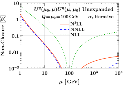
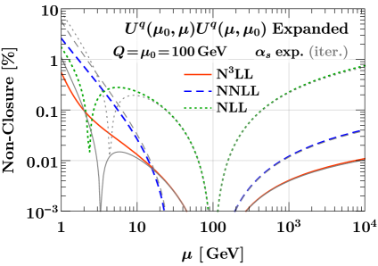
Figure -895: Deviation from the closure condition $U^{q}(\mu_{0},\mu)U^{q}(\mu,\mu_{0})=1$ for the quark evolution kernels from NLL to N³LL for the unexpanded method (left) and expanded method (right). For the expanded method, the gray lines show the result of using the iterative instead of the expanded $\alpha_{s}(\mu_{0})$.

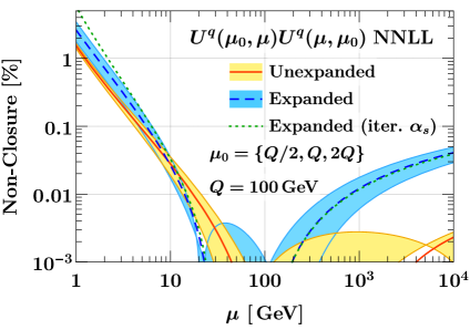
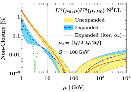
Figure -894: Deviation from the closure condition $U^{q}(\mu_{0},\mu)U^{q}(\mu,\mu_{0})=1$ at NNLL (left) and N³LL (right) for the unexpanded method (solid) and expanded method (dashed). The central lines are for $\mu_{0}=Q$, while the bands show the variation when changing $\mu_{0}$ to $Q/2$ and $2Q$. The green dotted line shows the result of using the iterative $\alpha_{s}(\mu_{0})$ in the expanded kernels (for $\mu_{0}=Q$ only).

By construction, the seminumerical and numerical methods satisfy the closure condition exactly, since they treat the integral and integration limits exactly. As already mentioned in subsection 3.5, the closure condition cannot be applied to the reexpanded method. We therefore only consider the unexpanded and expanded methods here. The reason these methods do not satisfy the closure condition exactly is due to the expansions in the integrand after the variable transformation from $\mu$ to $\alpha$, which means that the change of variables in the integration limits and the integrand are not in exact correspondence.

In figure -895, we compare the non-closure for the full quark evolution factor at different orders for the unexpanded (left panel) and expanded (right panel) methods. At LL, the integrals are trivially exact and satisfy exact closure, so we do not show them. At NLL, the non-closure can be quite sizeable, exceeding $\gtrsim 5\%$ when running to low scales. For the expanded kernels it even reaches $\sim 1\%$ when running to high scales. While the non-closure effect is reduced at higher orders, it can still reach $1-2\%$ at the lowest scales, and for the unexpanded kernels it does not reduce from NNLL to N³LL. For the expanded kernels, the non-closure reduces to below $1\%$ at N³LL, but this is likely accidental, since the expanded kernels are very sensitive to numerical cancellations when evolving to scales $\mu\lesssim 10\,\mathrm{GeV}$. This is evident when comparing the effect of using the iterative instead of the expanded solution for $\alpha_{s}(\mu_{0})$: Even a small change in $\alpha_{s}(\mu_{0})$ causes large changes in the observed level of non-closure.

In figure -894, we compare the unexpanded and expanded methods to each other at NNLL (left panel) and N³LL (right panel). In addition we vary $\mu_{0}$ away from $Q$ to $Q/2$ and $2Q$, as one would do in practical applications to estimate a resummation uncertainty. Here, this should however not be considered as an uncertainty estimate on the non-closure. Rather, it illustrates the effect of $\eta_{\Gamma}$, which contributes when $\mu_{0}\neq Q$, and the level at which the non-closure may influence such uncertainty estimates. The (non-)closure of the unexpanded kernels tends to be less sensitive to the choice of $\mu_{0}$ than the expanded ones.

Overall, we might say that the unexpanded kernels show a somewhat better closure behaviour. However, considering that at N³LL one is aiming for perturbative precision in the several percent range, their non-closure at this order is uncomfortably large.

For brevity we have only shown results for the quark evolution kernels here. The gluon evolution kernels have the same qualitative behaviour. The only difference is that the overall non-closure effect is about a factor of two larger for gluons than for quarks, corresponding to their larger color factor.

3.6.2 Approximation errors

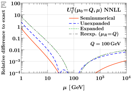
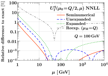
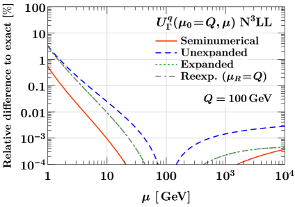
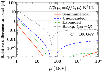
Figure -893: Deviation from the exact result for the quark cusp evolution kernel at NNLL (top) and N³LL (bottom) for all four approximate integration methods. On the left we use $\mu_{0}=Q$, for which the expanded and reexpanded kernels are equivalent. On the right we use $\mu_{0}=Q/2$, with $\mu_{R}=Q$ for the reexpanded method.

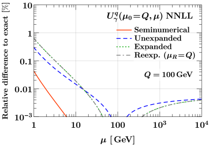
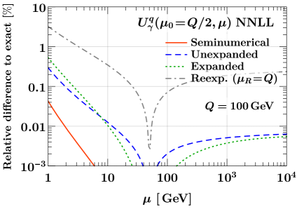
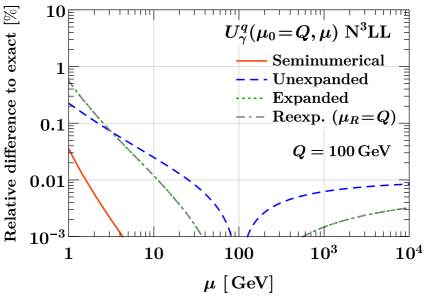
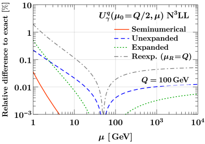
Figure -892: Same as figure -893, but for the quark noncusp evolution kernels.

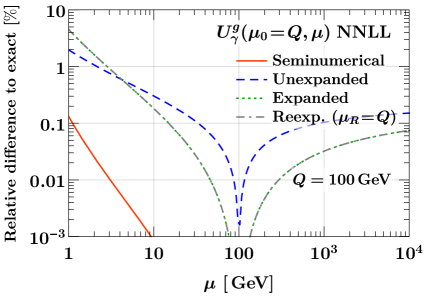
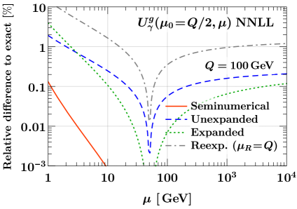
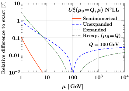
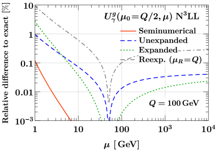
Figure -891: Same as figure -893, but for the gluon noncusp evolution kernels.

We now study the approximation errors of all four approximate methods relative to the exact numerical method. The results for the quark cusp contribution, $U^{q}_{\Gamma}$, are shown in figure -893, and for the quark and gluon noncusp contributions, $U^{q,g}_{\gamma}$, in figures -892 and -891. In all cases, we show the results at NNLL (top rows) and N³LL (bottom rows), and at $\mu_{0}=Q$ (left panels) and $\mu_{0}=Q/2$ (right panels).

At NNLL, we see a clear hierarchy, with the seminumerical method having the smallest approximation errors, followed by the unexpanded, and then the expanded methods, which is as expected given the increasing level of approximation involved in each method. At N³LL, the seminumerical method again performs best. The unexpanded and expanded kernels have similar errors for the cusp term, while the unexpanded ones fare better for the noncusp terms. The approximation error for the cusp term is always much larger than for the noncusp term, which is not surprising due to the additional $\ln(\mu)$ in its integrand. The errors for the gluon cusp contribution are about a factor of two larger than for quarks.

We find, somewhat surprisingly, that at NNLL the approximation error for the expanded kernels can exceed several percent when evolving to low scales, while at N³LL it still exceeds the percent level for both the unexpanded and expanded kernels alike. Overall, the picture is quantitatively quite similar to what we observed with the closure test.

We stress that the systematic differences we observe are solely due to the method of integrating the RGE for identical perturbative inputs. Typically, we would want such systematic effects to be much smaller than the perturbative precision we are aiming at, as was the case for the running of the coupling. In other words, we clearly want to avoid the method of integration to bias the result in any way. This is clearly not the case here, since at NNLL and N³LL one would typically aim at a perturbative precision of order several to few percent.

For $\mu_{0}=\mu_{R}=Q$, the reexpanded and expanded kernels are still equivalent. In the right panels, we therefore also show the results when reducing the hard scale of the evolution to $\mu_{0}=Q/2$. This has essentially no effect on the approximation error of the seminumerical, unexpanded, and expanded kernels. For the reexpanded kernels, we keep $\mu_{R}=Q$, which is a commonly used choice in resummation applications. The impact of treating the logarithms of $\mu_{0}/\mu_{R}$ and $Q/\mu_{0}$ at fixed-order in the reexpanded kernels compared to the expanded ones now becomes visible and turns out to be very large, which is quite unexpected. It easily exceeds the percent level even at N³LL, and not just for the cusp but even the noncusp contributions. For the cusp term, it exceeds $\gtrsim 10\%$ at the lowest scales. Note that roughly half of the observed difference is due to the reexpansion around $\alpha(\mu_{R})$ and half is due to the lower-order treatment of the $\eta_{\Gamma}$ term. This effect is not just due to the reduced amount of evolution from $Q/2$ to $\mu$, as that is present for all methods including the exact numerical result. Given the large numerical impact it has, it might be worthwhile to reconsider the reasons for performing this additional reexpansion around $\alpha(\mu_{R})$. Certainly, from the point of view of the evolution, the appropriate scale for $\alpha$ when starting the evolution from $\mu_{0}$ is $\mu_{0}$.

Of course, the differences due to the various approximations involved in all methods, including the reexpanded method, might be considered as higher-order effects. Nevertheless, given that they are not negligible or even exceed the perturbative precision they have to be addressed and accounted for. One option would be to include them as an additional systematic uncertainty in the theoretical uncertainty estimate. On the other hand, there is no fundamental theoretical reason for using any specific approximate solution. Hence, the best option would be to avoid incurring this additional uncertainty by using the unique exact solution of the defining RGE system resulting from the truncation of the perturbative series of the anomalous dimensions. If that is computationally prohibitive (or technically inconvenient), the seminumerical method offers a good compromise, since its approximation error is always well below the percent level, and so it is sufficiently accurate even for high-precision predictions.

4 Sudakov evolution kernels with two gauge interactions

Having investigated the integration of the one-dimensional kernels, we now consider the extension to two gauge interactions, in which case also mixed effects involving both gauge couplings $\alpha_{a,b}$ require resummation. In section 4.1, we review the general analytic structure for this case and the methods for evaluating them, based on what we learned from our exhaustive analysis of the one-dimensional case. We then present numerical results for the example of QCD$\otimes$QED in section 4.2.

4.1 Structure of the two-dimensional evolution kernel

We consider the Sudakov resummation for the direct product of two gauge groups $G_{a}\otimes G_{b}$. The extension to more groups is then straightforward. One key difference from the one-dimensional case is that the $\beta$ functions that govern the evolution of the couplings $\alpha_{a}$ and $\alpha_{b}$ now become a set of nonlinear coupled differential equations, as discussed in subsection 2.2.

The generic Sudakov RGE structure remains the same as in eq. (3.1), except that the perturbative expansions for all quantities now involve a double series in $\alpha_{a}$ and $\alpha_{b}$, including mixed terms corresponding to the emissions of two distinct gauge bosons. Hence, the all-order structure of the anomalous dimension is now given by

$$\gamma_{F}(\mu)=\frac{1}{\epsilon}\,\Gamma_{\mathrm{cusp}}[\alpha_{a}(\mu),\alpha_{b}(\mu)]\ln\frac{Q}{\mu}+\gamma[\alpha_{a}(\mu),\alpha_{b}(\mu)]\,,$$ (4.1)

with

$$\Gamma_{\mathrm{cusp}}(\alpha_{a},\alpha_{b}) \equiv\mathop{\sum_{n,m}}_{n+m\geq 1}\epsilon_{a}^{n}\epsilon_{b}^{n}\,\Gamma_{(n,m)}\Bigl{(}\frac{\alpha_{a}}{4\pi}\Bigr{)}^{n}\Bigl{(}\frac{\alpha_{b}}{4\pi}\Bigr{)}^{m}\,,$$ (4.2)

$$\gamma(\alpha_{a},\alpha_{b}) \equiv\mathop{\sum_{n,m}}_{n+m\geq 1}\epsilon_{a}^{n}\epsilon_{b}^{m}\,\gamma_{(n,m)}\Bigl{(}\frac{\alpha_{a}}{4\pi}\Bigr{)}^{n}\Bigl{(}\frac{\alpha_{b}}{4\pi}\Bigr{)}^{m}\,.$$ (4.3)

The bookkeeping parameters $\epsilon_{a,b}\equiv 1$ are the same as in the $\beta$ functions in eq. (2.2), and $\epsilon\sim\epsilon_{a}\sim\epsilon_{b}$, i.e. we make no assumption about the relative hierarchy of the two coupling constants. It is also important to note the correspondence to the typical notation for a single gauge theory $G_{a}$,

$$\Gamma_{n}\equiv\Gamma_{(n+1,0)}\,,\qquad\gamma_{n}\equiv\gamma_{(n+1,0)}$$ (4.4)

The Sudakov evolution kernel is given by the two-dimensional analogue of eq. (3.5),

$$U(\mu_{0},\mu)=\exp\biggl{\{}\int_{\mu_{0}}^{\mu}\frac{\mathrm{d}\mu^{\prime}}{\mu^{\prime}}\frac{1}{\epsilon}\,\Gamma_{\mathrm{cusp}}[\alpha_{a}(\mu^{\prime}),\alpha_{b}(\mu^{\prime})]\ln\frac{Q}{\mu^{\prime}}+\gamma[\alpha_{a}(\mu^{\prime}),\alpha_{b}(\mu^{\prime})]\biggr{\}}\,.$$ (4.5)

It is clear from eqs. (4.2) and (4.3) that the sums implicit in eq. (4.5) include pure $G_{a}$ terms $\mathcal{O}(\epsilon_{a}^{n})$, pure $G_{b}$ terms $\mathcal{O}(\epsilon^{m}_{b})$ terms, and mixed terms $\mathcal{O}(\epsilon^{n}_{a}\epsilon^{m}_{b})$.

4.2 Evaluation of the two-dimensional evolution kernel

Evaluating eq. (4.5) does not correspond to a simple extension of the single gauge interaction scenario, since mixed terms $\sim\mathcal{O}(\alpha_{a}\alpha_{b})$ appear in conjunction with the coupled $\beta$ functions.

The fully numerical method is of course still applicable, although it is even more computationally demanding now, since multiple coupled differential equations for $\alpha_{a,b}$ must be solved. As before we use the fully numerical method to provide the exact reference result to which other methods are compared.

The unexpanded analytic method is not easily extendable, since the coupled $\beta$ functions do not allow an analogous change of variables along the lines of of $\mathrm{d}\ln\mu\rightarrow\mathrm{d}\alpha_{a}/\beta^{a}(\alpha_{a},\alpha_{b})$, because of the dependence on the second coupling. Doing so would require one to express the $\mu$ dependence of $\alpha_{b}$ in terms of $\alpha_{a}$, which in turn requires that one treats $\alpha_{b}$ as in the expanded analytic method, at which point the advantage of the unexpanded method is lost. In principle, this could still be an option for cases where there is a clear hierarchy between two couplings to justify treating them on unequal footing, as would be the case for QCD$\otimes$QED. However, we do not pursue this option further here for the reasons given below.

The expanded analytic method can still be applied to evaluate eq. (4.5). This is achieved by using the expanded solution of the coupled $\beta$ RGE for $\alpha_{a}$ and $\alpha_{b}$ obtained from eq. (2.2), substituting it into the perturbative expansions of the anomalous dimensions, and then explicitly performing the integration in terms of $\ln\mu$. This was done in ref. [35].

In either case, the obtained analytic kernels will inevitably suffer from the same-sized approximation errors already seen in the pure QCD case in subsection 3.6. The generalization to the product group $G_{a}\otimes G_{b}$ does not alter the ultimate source, which are the additional approximation(s) made in the integrand. By including EW or QED corrections, one is looking for percent-level effects, and based on our findings and discussion in the previous section, the analytic methods do not appear to provide sufficient numerical accuracy.

We therefore take the seminumerical method as our method of choice for evaluating the two-dimensional evolution kernels. As already seen in subsection 3.6, it features exact closure and very small approximation errors (well below the percent-level at NNLL), at a reasonable computational cost. The extension to the two-dimensional case eq. (4.5) only requires two steps:

1. We solve the coupled $\beta$ functions in eq. (2.2) via the iterative method, up to the required order in $\epsilon$, which yields the closed-form analytic expressions for $\alpha_{a}(\mu)$ and $\alpha_{b}(\mu)$ in eq. (2.2).

2. We then evaluate the evolution kernel $U(\mu,\mu_{0})$ by employing a numerical integration routine in eq. (4.5), using the analytic expressions for $\alpha_{a,b}(\mu)$ obtained in step 1 in the integrand.

Schematically, this procedure is illustrated by

$$U(\mu_{0},\mu)=\exp\biggl{\{}\underbrace{\int_{\mu_{0}}^{\mu}\frac{\mathrm{d}\mu^{\prime}}{\mu^{\prime}}}_{\text{numerical}}\sum_{\begin{subarray}{c}n,m\\ n+m\geq 1\end{subarray}}\biggl{[} \frac{\epsilon_{a}^{n}\epsilon_{b}^{m}}{\epsilon}\Gamma_{(n,m)}\overbrace{\Bigl{(}\frac{\alpha_{a}(\mu^{\prime})}{4\pi}\Bigr{)}^{n}\Bigl{(}\frac{\alpha_{b}(\mu^{\prime})}{4\pi}\Bigr{)}^{m}}^{{\color[rgb]{0,0,1}{\text{eq.~{}\eqref{eq:2DalphaaNNLO}}}}}\ln\frac{Q}{\mu^{\prime}}$$

$$+\epsilon_{a}^{n}\epsilon_{b}^{m}\gamma_{(n,m)}\underbrace{\Bigl{(}\frac{\alpha_{a}(\mu^{\prime})}{4\pi}\Bigr{)}^{n}\Bigl{(}\frac{\alpha_{b}(\mu^{\prime})}{4\pi}\Bigr{)}^{m}}_{\color[rgb]{0,0,1}{\text{eq.~{}\eqref{eq:2DalphaaNNLO}}}}\biggr{]}\biggr{\}}\,.$$ (4.6)

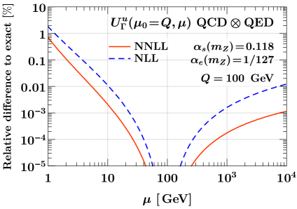
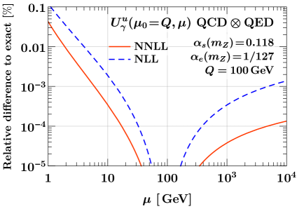
Figure -890: Deviation of the seminumerical kernels from the exact result for the joint QCD$\otimes$QED $u$-quark evolution kernel at NLL (dashed) and NNLL (solid). The cusp contribution is shown on the left and the noncusp contribution on the right.

In what follows, we apply this method to the mixed gauge QCD$\otimes$QED scenario. We consider the $u\bar{u}$ hard function as a concrete example. The relevant coefficients up to three loops can be found in appendices A.2 and A.3, allowing us to obtain the complete NNLL joint QCD$\otimes$QED Sudakov evolution.

In figure -890, we show the approximation errors for the seminumerical method at NLL and NNLL for the cusp (left panel) and noncusp (right panel) contributions. As for the pure QCD case, the former has a larger approximation error, while overall it remains well below 1% everywhere (except at NLL for the cusp term at the very lowest $\mu$ values).

In figure -889, we show the relative impact of the QED corrections by comparing the full QCD$\otimes$QED to the pure QCD resummation kernels at each order. For the cusp piece (left panel) the impact reaches $4-5\%$ over two decades of evolution, while for the noncusp piece (right panel) it reaches close to $1\%$. The overall effect for QED is expectedly small due to the smallness of the electromagnetic coupling. Considering a toy QCD$\otimes$QED^′ model with $\alpha_{e}^{\prime}(m_{Z})=0.1$ in figure -888, the corrections become much larger, $30-50\%$ for the cusp piece and $5-15\%$ for the noncusp piece. Note that the impact is driven not only by pure QED and mixed corrections in the expansion of the anomalous dimensions, but also by the effects induced by the mixed $\beta$ functions in the coupling evolution. Note also that the impact for the cusp term is practically identical at NLL and NNLL even for QED^′. This is somewhat accidental and due to the fact that the cusp anomalous dimension does not yet receive any mixed contributions at three loops while its pure QCD and QED three-loop coefficients happen to be very small.

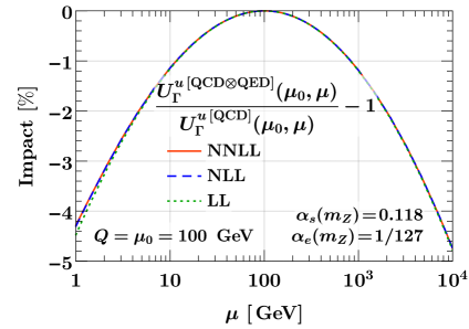
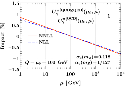
Figure -889: Impact of the QED corrections on the $u$-quark Sudakov evolution kernel at LL, NLL, and NNLL for the cusp (left panel) and noncusp (right panel) contributions. We show the relative difference of the full QCD$\otimes$QED evolution to the pure QCD case at the corresponding order.

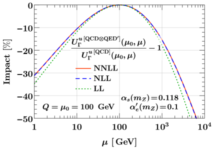
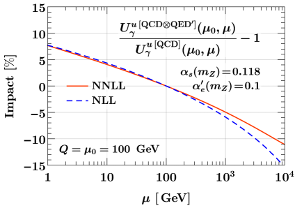
Figure -888: Same as figure -889, but for a toy QED^′ with $\alpha_{e}^{\prime}(m_{Z})=0.1$.

5 Conclusions

High-precision experimental measurements of (e.g.) $W$ and $Z$ production at the LHC at the (sub-)percent level, as well as future measurements at the high-luminosity LHC or future high-energy colliders, demand equally precise resummed predictions in QCD$\otimes$EW. In this paper we studied the technical aspects of achieving this joint resummation at higher orders in generic coupled gauge environments.

In particular, at the level of the Sudakov evolution kernel appearing in any resummation formalism, we showed that the commonly used methods of evaluating the associated integrals in the Sudakov exponent via analytic approximations can cause numerical differences of the same size as the contributions coming from moving to a higher logarithmic accuracy or including EW radiation. In other words, systematic integration errors that are typically assumed to be subleading cannot be overlooked when attempting percent-level precision.

To show this we first studied five methods for integrating the evolution kernels in the case of a single gauge interaction: numerical, seminumerical, unexpanded analytic, expanded analytic, and reexpanded analytic. Their main difference is in the treatment of the $\mu$ dependence of $\alpha(\mu)$ that one has to integrate over. Although all methods employ a priori justifiable assumptions, we showed that the latter three analytic methods can introduce errors at and above the percent-level compared to the exact result (obtained via a fully numerical treatment at a sufficiently high numerical precision). One should therefore be cautious in using them, since their approximation errors can be nonnegligible compared to the perturbative precision one is aiming for. The reexpanded kernels, which are often used in the literature, are particularly notable; differences greater than $10\%$ are possible over only two decades of evolution.

On the other hand, we found that a seminumerical method, which combines an accurate analytic approximation for the running of the couplings with a numerical integration, yielded minimal errors (typically $\leq 0.1\%$), while still maintaining reasonable computing times. We therefore advocate its use for phenomenological studies at high precision and in joint resummation environments. As an example, we have used it to obtain the complete NNLL QCD$\otimes$QED Sudakov evolution factor.

Appendix A Perturbative results

In this appendix we summarize the results for the higher-order analytic RGE solutions, and the coefficients of the QCD and QED $\beta$ functions and anomalous dimensions.

A.1 RGE solutions

The iterative solution of the $\beta$-function RGE up to N³LO, $\mathcal{O}(\epsilon^{3})$, reads

$$\frac{\alpha(\mu_{0})}{\alpha(\mu)} =X+\epsilon\,\frac{\alpha(\mu_{0})}{4\pi}\,b_{1}\ln X+\epsilon^{2}\,\frac{\alpha(\mu_{0})^{2}}{(4\pi)^{2}}\biggl{(}b_{2}\,\frac{X-1}{X}+b_{1}^{2}\,\frac{1-X+\ln X}{X}\biggr{)}$$

$$\quad+\epsilon^{3}\,\frac{\alpha(\mu_{0})^{3}}{(4\pi)^{3}}\biggl{[}b_{3}\,\frac{X^{2}-1}{2X^{2}}+b_{2}b_{1}\Bigl{(}\frac{1-X}{X}+\frac{\ln X}{X^{2}}\Bigr{)}+b_{1}^{3}\,\frac{(1-X)^{2}-\ln^{2}X}{2X^{2}}\biggr{]}\,,$$ (A.1)

where $b_{n}=\beta_{n}/\beta_{0}$ and $X=1+\frac{\alpha(\mu_{0})}{2\pi}\,\beta_{0}\,\ln(\mu/\mu_{0})$ as in eq. (2.3).

The functions $K_{\Gamma}$, $\eta_{\Gamma}$, and $K_{\gamma}$ appearing in the unexpanded analytic Sudakov exponents in eq. (3.12) are given up to N³LL, $\mathcal{O}(\epsilon^{3})$, by

$$K_{\Gamma}(\mu_{0},\mu) =-\frac{\Gamma_{0}}{4\beta_{0}^{2}}\biggl{\{}\frac{4\pi}{\alpha(\mu_{0})}\Bigl{(}1-\frac{1}{r}-\ln r\Bigr{)}+\epsilon\Bigl{[}(\hat{\Gamma}_{1}-b_{1})(1-r+\ln r)+\frac{b_{1}}{2}\ln^{2}r\Bigr{]}$$

$$\quad+\epsilon^{2}\,\frac{\alpha(\mu_{0})}{4\pi}\biggl{[}(b_{1}^{2}-b_{2})\Bigl{(}\frac{1-r^{2}}{2}+\ln r\Bigr{)}+(b_{1}\hat{\Gamma}_{1}-b_{1}^{2})(1-r+r\ln r)$$

$$\qquad-(\hat{\Gamma}_{2}-b_{1}\hat{\Gamma}_{1})\frac{(1-r)^{2}}{2}\biggr{]}+\epsilon^{3}\,\frac{\alpha(\mu_{0})^{2}}{(4\pi)^{2}}\biggl{[}(b_{2}-b_{1}^{2})(\hat{\Gamma}_{1}-b_{1})\frac{(1-r)^{2}(2+r)}{3}$$

$$\qquad+(\hat{\Gamma}_{3}-b_{3}-b_{1}(\hat{\Gamma}_{2}-b_{2}))\Bigl{(}\frac{1-r^{3}}{3}-\frac{1-r^{2}}{2}\Bigr{)}$$

$$\qquad+b_{1}(\hat{\Gamma}_{2}-b_{2}-b_{1}(\hat{\Gamma}_{1}-b_{1}))\Bigl{(}\frac{1-r^{2}}{4}+\frac{r^{2}\ln r}{2}\Bigr{)}$$

$$\qquad+(-b_{3}+2b_{1}b_{2}-b_{1}^{3})\Bigl{(}\frac{1-r^{2}}{4}+\frac{\ln r}{2}\Bigr{)}\biggr{]}\biggr{\}}\,,$$ (A.2)

$$\eta_{\Gamma}(\mu_{0},\mu) =-\frac{\Gamma_{0}}{2\beta_{0}}\biggl{[}\ln r+\epsilon\,\frac{\alpha(\mu_{0})}{4\pi}(\hat{\Gamma}_{1}-b_{1})(r-1)+\epsilon^{2}\,\frac{\alpha(\mu_{0})^{2}}{(4\pi)^{2}}(\hat{\Gamma}_{2}-b_{1}\hat{\Gamma}_{1}+b_{1}^{2}-b_{2})\frac{r^{2}-1}{2}$$

$$\quad+\epsilon^{3}\,\frac{\alpha(\mu_{0})^{3}}{(4\pi)^{3}}\Bigl{[}\hat{\Gamma}_{3}-b_{3}-b_{1}(\hat{\Gamma}_{2}-b_{2})+(b_{1}^{2}-b_{2})(\hat{\Gamma}_{1}-b_{1})\Bigr{]}\frac{r^{3}-1}{3}\biggr{]}\,,$$ (A.3)

$$K_{\gamma}(\mu_{0},\mu) =-\frac{\gamma_{0}}{2\beta_{0}}\biggl{[}\epsilon\ln r+\epsilon^{2}\,\frac{\alpha(\mu_{0})}{4\pi}(\hat{\gamma}_{1}\!-\!b_{1})(r\!-\!1)+\epsilon^{3}\,\frac{\alpha(\mu_{0})^{2}}{(4\pi)^{2}}(\hat{\gamma}_{2}-b_{1}\hat{\gamma}_{1}+b_{1}^{2}-b_{2})\frac{r^{2}\!-\!1}{2}\biggr{]},$$ (A.4)

where $b_{n}=\beta_{n}/\beta_{0}$, $\hat{\Gamma}_{n}=\Gamma_{n}/\Gamma_{0}$, $\hat{\gamma}_{n}=\gamma_{n}/\gamma_{0}$, and $r=\alpha_{s}(\mu)/\alpha_{s}(\mu_{0})$.

The corresponding kernels for the expanded analytic method are obtained by inserting eq. (A.1) into the above and expanding the results to $\mathcal{O}(\epsilon^{3})$.

A.2 QCD anomalous dimensions

Here we collect the pure QCD anomalous dimensions. For clarity and to avoid any confusion we use the two-dimensional notation everywhere. The QCD $\beta$-function coefficients in the $\overline{\text{MS}}$ scheme up to 3 loops are [59, 60]

$$\beta^{s}_{00}\equiv\beta_{0} =\frac{11}{3}\,C_{A}-\frac{4}{3}\,T_{F}\,n_{f}\,,$$

$$\beta^{s}_{10}\equiv\beta_{1} =\frac{34}{3}\,C_{A}^{2}-2T_{F}\,n_{f}\Bigl{(}\frac{10}{3}\,C_{A}+2C_{F}\Bigr{)}\,,$$ (A.5)

$$\beta^{s}_{20}\equiv\beta_{2} =\frac{2857}{54}\,C_{A}^{3}+2T_{F}\,n_{f}\Bigl{(}-\frac{1415}{54}\,C_{A}^{2}-\frac{205}{18}\,C_{F}C_{A}+C_{F}^{2}\Bigr{)}+4T_{F}^{2}\,n_{f}^{2}\Bigl{(}\frac{79}{54}\,C_{A}+\frac{11}{9}\,C_{F}\Bigr{)}.$$

The four-loop coefficient for $N_{c}=3$ is given by [61, 62]

$$\beta^{s}_{30}\equiv\beta_{3}=\Bigl{(}\frac{149753}{6}+3564\zeta_{3}\Bigr{)}-\Bigl{(}\frac{1078361}{162}+\frac{6508}{27}\zeta_{3}\Bigr{)}n_{f}+\Bigl{(}\frac{50065}{162}+\frac{6472}{81}\zeta_{3}\Bigr{)}n_{f}^{2}+\frac{1093}{729}n_{f}^{3}.$$ (A.6)

The $\overline{\text{MS}}$ quark cusp anomalous dimension coefficients up to three loops are [63, 64]

$$\Gamma^{q}_{(1,0)}\equiv\Gamma^{q}_{0} =4C_{F}\,,$$

$$\Gamma^{q}_{(2,0)}\equiv\Gamma^{q}_{1} =4C_{F}\biggl{[}C_{A}\Bigl{(}\frac{67}{9}-\frac{\pi^{2}}{3}\Bigr{)}-\frac{20}{9}\,T_{F}\,n_{f}\biggr{]}\,,$$ (A.7)

$$\Gamma^{q}_{(3,0)}\equiv\Gamma^{q}_{2} =4C_{F}\biggl{\{}C_{A}^{2}\Bigl{(}\frac{245}{6}-\frac{134\pi^{2}}{27}+\frac{11\pi^{4}}{45}+\frac{22\zeta_{3}}{3}\Bigr{)}$$

$$\qquad\quad+2T_{F}\,n_{f}\biggl{[}C_{A}\Bigl{(}-\frac{209}{27}+\frac{20\pi^{2}}{27}-\frac{28\zeta_{3}}{3}\Bigr{)}+C_{F}\Bigl{(}-\frac{55}{6}+8\zeta_{3}\Bigr{)}\biggr{]}-\frac{16}{27}\,T_{F}^{2}\,n_{f}^{2}\biggr{\}}.$$

The four-loop coefficient entering at N³LL has become available during recent years, see e.g. refs. [65, 66, 67, 68, 69]. We use the numerical result for $N_{c}=3$ and $n_{f}=5$ obtained from ref. [69],

$$\Gamma^{q}_{(4,0)}\equiv\Gamma^{q}_{3}=104.93\,C_{F}\,.$$ (A.8)

Finally, the $\overline{\text{MS}}$ noncusp quark anomalous dimension coefficients for the hard function up to three loops are [70, 71, 72]

$$\gamma^{q}_{H\,(1,0)}\equiv\gamma^{q}_{H\,0} =-6C_{F}\,,$$

$$\gamma^{q}_{H\,(2,0)}\equiv\gamma^{q}_{H\,1} =-2C_{F}\biggl{[}C_{A}\Bigl{(}\frac{41}{9}-26\zeta_{3}\Bigr{)}+C_{F}\Bigl{(}\frac{3}{2}-2\pi^{2}+24\zeta_{3}\Bigr{)}+\beta_{0}\Bigl{(}\frac{65}{18}+\frac{\pi^{2}}{2}\Bigr{)}\biggr{]}\,,$$

$$\gamma^{q}_{H\,(3,0)}\equiv\gamma^{q}_{H\,2} =-2C_{F}\biggl{[}C_{A}^{2}\Bigl{(}\frac{66167}{324}-\frac{686\pi^{2}}{81}-\frac{302\pi^{4}}{135}-\frac{782\zeta_{3}}{9}+\frac{44\pi^{2}\zeta_{3}}{9}+136\zeta_{5}\Bigr{)}$$

$$\qquad\qquad+C_{F}C_{A}\Bigl{(}\frac{151}{4}-\frac{205\pi^{2}}{9}-\frac{247\pi^{4}}{135}+\frac{844\zeta_{3}}{3}+\frac{8\pi^{2}\zeta_{3}}{3}+120\zeta_{5}\Bigr{)}$$

$$\qquad\qquad+C_{F}^{2}\Bigl{(}\frac{29}{2}+3\pi^{2}+\frac{8\pi^{4}}{5}+68\zeta_{3}-\frac{16\pi^{2}\zeta_{3}}{3}-240\zeta_{5}\Bigr{)}$$ (A.9)

$$\qquad\qquad+C_{A}\beta_{0}\Bigl{(}-\frac{10781}{108}+\frac{446\pi^{2}}{81}+\frac{449\pi^{4}}{270}-\frac{1166\zeta_{3}}{9}\Bigr{)}$$

$$\qquad\qquad+\beta_{1}\Bigl{(}\frac{2953}{108}-\frac{13\pi^{2}}{18}-\frac{7\pi^{4}}{27}+\frac{128\zeta_{3}}{9}\Bigr{)}+\beta_{0}^{2}\Bigl{(}-\frac{2417}{324}+\frac{5\pi^{2}}{6}+\frac{2\zeta_{3}}{3}\Bigr{)}\biggr{]}\,.$$

The corresponding gluon noncusp anomalous dimensions can be found e.g. in appendix A.2 of ref. [45].

A.3 QED and mixed QCD$\otimes$QED anomalous dimensions

Here we collect all QED and QCD$\otimes$QED coefficients that are required for the full NNLL hard evolution, and which enter in the numerical results in subsection 2.2 and section 4. The mixed QCD $\beta$-function coefficients to three loops are

$$\beta_{01}^{s} =-4T_{F}\,\overline{Q^{2}}\,,$$

$$\beta_{02}^{s} =\frac{44}{9}\,T_{F}\,\overline{Q^{2}}\bigl{(}N_{c}\,\overline{Q^{2}}+n_{\ell}\,Q^{2}_{\ell}\bigr{)}+2T_{F}\,\overline{Q^{4}}\,,$$

$$\beta_{11}^{s} =(4C_{F}-8C_{A})\,T_{F}\,\overline{Q^{2}}\,,$$ (A.10)

while the pure and mixed QED $\beta$-function coefficients up to three loops are

$$\beta_{00}^{e} =\frac{4}{3}\bigl{(}N_{c}\,\overline{Q^{2}}+n_{\ell}\,Q^{2}_{\ell}\bigr{)}\,,$$

$$\beta_{10}^{e} =4\bigl{(}N_{c}\,\overline{Q^{4}}+n_{\ell}\,Q^{4}_{\ell}\bigr{)}\,,$$

$$\beta_{20}^{e} =-\frac{44}{9}\bigl{(}N_{c}\,\overline{Q^{4}}+n_{\ell}\,Q_{\ell}^{4}\bigr{)}\bigl{(}N_{c}\,\overline{Q^{2}}+n_{\ell}\,Q^{2}_{\ell}\bigr{)}-2\bigl{(}N_{c}\,\overline{Q^{6}}+n_{\ell}\,Q_{\ell}^{6}\bigr{)}\,,$$ (A.11)

$$\beta_{01}^{e} =4C_{F}\,N_{c}\,\overline{Q^{2}}\,,$$

$$\beta_{02}^{e} =\Bigl{(}\frac{133}{18}C_{A}-C_{F}\Bigr{)}2C_{F}\,N_{c}\,\overline{Q^{2}}-\frac{44}{9}\,C_{F}\,T_{F}\,n_{f}\,N_{c}\,\overline{Q^{2}}\,,$$

$$\beta_{11}^{e} =-4\,C_{F}\,N_{c}\,\overline{Q^{4}}\,.$$ (A.12)

Here we defined

$$\overline{Q^{n}}=\sum_{q}Q_{q}^{n}\,,$$ (A.13)

where the sum runs over the active quark flavors with $Q_{u,c}=2/3$ and $Q_{d,s,b}=-1/3$ the quark charges, $N_{c}=3$ the number of colors, $Q_{\ell}=-1$ the lepton charge, and $n_{\ell}=3$ the number of charged leptons. The extraction of the three-loop mixed coefficients is discussed in appendix B.

The QED coefficients for the cusp anomalous dimension are obtained straightforwardly by taking the abelian QED limit of eq. (A.2),

$$\Gamma^{q}_{(0,1)} =4Q_{q}^{2}\,,$$

$$\Gamma^{q}_{(0,2)} =4Q_{q}^{2}\Bigl{[}-\frac{20}{9}\bigl{(}N_{c}\,\overline{Q^{2}}+n_{\ell}\,Q_{\ell}^{2}\bigr{)}\Bigr{]}\,,$$

$$\Gamma^{q}_{(0,3)} =4Q_{q}^{2}\biggl{[}Q_{q}^{2}\bigl{(}N_{c}\,\overline{Q^{2}}+n_{\ell}\,Q_{\ell}^{2}\bigr{)}\Bigl{(}-\frac{55}{3}+16\zeta_{3}\Bigr{)}-\frac{16}{27}\bigl{(}N_{c}\,\overline{Q^{2}}+n_{\ell}\,Q_{\ell}^{2}\bigr{)}^{2}\biggr{]}\,.$$ (A.14)

Up to three loops, the mixed coefficients vanish, as was noted in ref. [7],

$$\Gamma^{q}_{(1,1)}=\Gamma^{q}_{(1,2)}=\Gamma^{q}_{(2,1)}=0\,.$$ (A.15)

A nonzero mixed contribution is expected to first appear at four loops.

The noncusp anomalous dimensions are

$$\gamma^{q}_{H\,(0,1)} =-6Q_{q}^{2}\,,$$

$$\gamma^{q}_{H\,(0,2)} =-2Q_{q}^{2}\biggl{[}Q_{q}^{2}\Bigl{(}\frac{3}{2}-2\pi^{2}+24\zeta_{3}\Bigr{)}-\bigl{(}N_{c}\,\overline{Q^{2}}+n_{\ell}\,Q^{2}_{\ell}\bigr{)}\Bigl{(}\frac{130}{27}+\frac{2\pi^{2}}{3}\Bigr{)}\biggr{]}\,,$$

$$\gamma^{q}_{H(1,1)} =-2Q_{q}^{2}\,C_{F}\,(3-4\pi^{2}+48\zeta_{3})\,.$$ (A.16)

The pure QED coefficients are given by the abelian QED limit of the QCD coefficients in eq. (A.2). The result for the mixed two-loop coefficient, $\gamma^{q}_{H(1,1)}$, is obtained by following the abelianization procedure in ref. [32], and agrees with that given in ref. [36].

Appendix B Extraction of three-loop mixed QCD$\otimes$QED coefficients

In this section, we discuss our extraction of the three-loop coefficients of the mixed QCD$\otimes$QED $\beta$ functions from the results in ref. [37], which are required for the complete NNLO running.

Ref. [37] considers the coupled $\beta$-function RGE for a generic gauge group given as the product of $n$ simple groups, $G=G_{1}\otimes G_{2}\otimes\dots\otimes G_{n}$. They explicitly calculate the case of three distinct simple groups $G=G_{1}\otimes G_{2}\otimes G_{3}$, since at most three gauge bosons can propagate simultaneously at three loops. They consider the case where each simple group $G_{i}$ is nonabelian, but it is straightforward to apply their results to the abelian case by a proper modification of the Casimir invariants.

To obtain the QCD$\otimes$QED coefficients, we specify ourselves to the product group $G=SU(3)_{c}\otimes U(1)_{EM}\otimes\mathbf{1}$, where $\mathbf{1}$ is the trivial identity group. In addition, we only keep fermionic matter couplings, setting the Yukawa and scalar (quartic) couplings and the Casimir invariants of the scalar representation $S$ to zero, as they appear in eq. (3.1) of ref. [37]. We have explicitly checked that with this procedure we reproduce the pure QCD $\beta$-function coefficients.

Since we only have two couplings, namely $\alpha_{i}$ with $i=s,e$ for QCD and QED respectively, the usual Casimir invariants for the $SU(3)_{c}$ gauge group are

$$[T_{F}^{A},T_{F}^{B}] =\mathrm{i}f^{ABC}T_{F}^{C}\,\,,$$

$$\operatorname{Tr}T_{F}^{A}T_{F}^{B} =\delta^{AB}\,T(F_{s})\,,$$

$$(T_{F}^{A})_{ab}(T_{F}^{A})_{bc} =\delta_{ac}\,C(F_{s})\,,$$

$$f^{ABC}f^{DBC} =\delta^{AD}\,C(G_{s})\,,$$

$$\delta^{AA} =d(G_{s})\,,$$ (B.1)

where $F_{s}$ and $G_{s}$ stand for the fundamental and adjoint representations, so $C(F_{s})\equiv C_{F}$ and $C(G_{s})\equiv C_{A}$. For the case of $U(1)_{EM}$, we take the abelian limit

$$C(F_{e})\rightarrow Q_{f}^{2}\,,\qquad T(F_{e})\rightarrow Q_{f}^{2}\,,\qquad C(G_{e})\rightarrow 0\,,$$ (B.2)

with $f$ representing quarks and leptons. Note that sums over fermion species do appear in the $\beta$-function coefficients that each gauge group involves, i.e. quarks for $SU(3)_{c}$ and both quarks and leptons for $U(1)_{EM}$. Also, since ref. [37] decomposes Dirac fermions into chiral fermions, we have to substitute $n_{f}\rightarrow 2n_{f}$ for the number of quarks and $n_{\ell}\rightarrow 2n_{\ell}$ for the number of leptons in their results.

All of this considered, the $\beta^{e}_{11}$ coefficient can be extracted from the generic results of ref. [37], finding

$$\beta^{e}_{11}=\sum_{F}2[2C(G_{i})-C(F_{i})]T(F_{i})C(F_{j})D(F_{ij})D(F_{i})\,,$$ (B.3)

where $i=e$, since we are considering the $U(1)_{EM}$ $\beta$ function, and $j=s$. These specifications then give

$$\beta^{e}_{11} =-2\sum_{F=q,\ell}C(F_{e})T(F_{e})C(F_{s})D(F_{es})D(F_{e})=-4C_{F}\,\overline{Q^{4}}\,N_{c}\,,$$ (B.4)

where the fermion sum over the leptons does not contribute due to the presence of $C(\ell_{s})=0$ and the multiplicity factors

$$D(F_{es})=\prod_{k\neq e,s}\,d(F_{k})=d(\mathbf{1})=1\,,\qquad D(F_{e})=\displaystyle\prod_{k\neq e}\,d(F_{k})=d(F_{s})\,d(\mathbf{1})=N_{c}$$ (B.5)

in our case correspond to the dimension of the trivial group factor and of the fundamental $SU(3)_{c}$ representation.

We can also read off the $\beta^{e}_{02}$ coefficient

$$\beta^{e}_{02} =\sum_{F}\Bigl{(}\frac{133}{18}C(G_{j})-C(F_{j})\Bigr{)}C(F_{j})T(F_{i})D(F_{ij})D(F_{i})$$

$$\quad-\sum_{F_{m},F_{n}}\frac{11}{9}C(F_{m,j})T(F_{n,j})T(F_{m,i})D(F_{m,ij})D(F_{n,j})D(F_{m,i})\,,$$ (B.6)

where again $i=e$ and $j=s$. We therefore find

$$\beta^{e}_{02} =\Bigl{(}\frac{133}{18}C_{A}-C_{F}\Bigr{)}C_{F}\,2\overline{Q^{2}}\,d(\mathbf{1})N_{c}-\sum_{F_{m}}\frac{11}{9}C(F_{m,s})T(F_{m,e})D(F_{m,es})D(F_{m,e})(2\,T_{F}\,n_{f})$$

$$=\Bigl{(}\frac{133}{18}C_{A}-C_{F}\Bigr{)}2C_{F}\,N_{c}\,\overline{Q^{2}}-\frac{44}{9}\,C_{F}\,T_{F}\,n_{f}\,N_{c}\,\overline{Q^{2}}\,.$$ (B.7)

Observe that again only the sum over quarks contributes, since the leptonic sums include a $C(\ell_{s})=T(\ell_{s})=0$.

Following the same procedure we also obtained the mixed QCD coefficients $\beta^{s}_{11}$ and $\beta^{s}_{02}$ as given in eq. (A.3), in agreement with the corresponding results given in ref. [76], where $\beta_{11}^{s}$ was obtained from an explicit three-loop calculation.

References

- [1] P. Ciafaloni and D. Comelli, Sudakov enhancement of electroweak corrections, Phys. Lett. B446 (1999) 278 [hep-ph/9809321].
- [2] V. S. Fadin, L. N. Lipatov, A. D. Martin and M. Melles, Resummation of double logarithms in electroweak high-energy processes, Phys. Rev. D61 (2000) 094002 [hep-ph/9910338].
- [3] J. H. Kuhn, A. A. Penin and V. A. Smirnov, Summing up subleading Sudakov logarithms, Eur. Phys. J. C17 (2000) 97 [hep-ph/9912503].
- [4] B. Jantzen, J. H. Kuhn, A. A. Penin and V. A. Smirnov, Two-loop electroweak logarithms in four-fermion processes at high energy, Nucl. Phys. B731 (2005) 188 [hep-ph/0509157].
- [5] A. Denner, B. Jantzen and S. Pozzorini, Two-loop electroweak next-to-leading logarithmic corrections to massless fermionic processes, Nucl. Phys. B761 (2007) 1 [hep-ph/0608326].
- [6] J.-y. Chiu, F. Golf, R. Kelley and A. V. Manohar, Electroweak Corrections in High Energy Processes using Effective Field Theory, Phys. Rev. D77 (2008) 053004 [0712.0396].
- [7] J.-y. Chiu, R. Kelley and A. V. Manohar, Electroweak Corrections using Effective Field Theory: Applications to the LHC, Phys. Rev. D78 (2008) 073006 [0806.1240].
- [8] G. Bell, J. H. Kuhn and J. Rittinger, Electroweak Sudakov Logarithms and Real Gauge-Boson Radiation in the TeV Region, Eur. Phys. J. C70 (2010) 659 [1004.4117].
- [9] T. Becher and X. Garcia i Tormo, Electroweak Sudakov effects in and production at large transverse momentum, Phys. Rev. D88 (2013) 013009 [1305.4202].
- [10] J. R. Christiansen and T. Sjöstrand, Weak Gauge Boson Radiation in Parton Showers, JHEP 04 (2014) 115 [1401.5238].
- [11] F. Krauss, P. Petrov, M. Schoenherr and M. Spannowsky, Measuring collinear W emissions inside jets, Phys. Rev. D89 (2014) 114006 [1403.4788].
- [12] S. Jadach, B. F. L. Ward, Z. A. Was and S. A. Yost, KK MC-hh: Resumed exact O(L) EW corrections in a hadronic MC event generator, Phys. Rev. D94 (2016) 074006 [1608.01260].
- [13] C. W. Bauer, N. Ferland and B. R. Webber, Standard Model Parton Distributions at Very High Energies, JHEP 08 (2017) 036 [1703.08562].
- [14] A. V. Manohar and W. J. Waalewijn, Electroweak Logarithms in Inclusive Cross Sections, JHEP 08 (2018) 137 [1802.08687].
- [15] M. L. Mangano et al., Physics at a 100 TeV pp Collider: Standard Model Processes, CERN Yellow Rep. (2017) 1 [1607.01831].
- [16] ATLAS collaboration, Measurement of the boson transverse momentum distribution in collisions at = 7 TeV with the ATLAS detector, JHEP 09 (2014) 145 [1406.3660].
- [17] ATLAS collaboration, Measurement of the transverse momentum and distributions of Drell-Yan lepton pairs in proton-proton collisions at TeV with the ATLAS detector, Eur. Phys. J. C76 (2016) 291 [1512.02192].
- [18] ATLAS collaboration, Measurement of the -boson mass in pp collisions at TeV with the ATLAS detector, Eur. Phys. J. C78 (2018) 110 [1701.07240].
- [19] CMS collaboration, Measurement of the differential and double-differential Drell-Yan cross sections in proton-proton collisions at 7 TeV, JHEP 12 (2013) 030 [1310.7291].
- [20] CMS collaboration, Measurement of the Z boson differential cross section in transverse momentum and rapidity in proton-proton collisions at 8 TeV, Phys. Lett. B749 (2015) 187 [1504.03511].
- [21] CMS collaboration, Measurements of differential Z boson production cross sections in pp collisions with CMS at , Tech. Rep. CMS-PAS-SMP-17-010, CERN, Geneva, 2019.
- [22] S. Dittmaier, A. Huss and C. Schwinn, Dominant mixed QCD-electroweak O(s) corrections to Drell-Yan processes in the resonance region, Nucl. Phys. B904 (2016) 216 [1511.08016].
- [23] S. Alioli et al., Precision studies of observables in and processes at the LHC, Eur. Phys. J. C77 (2017) 280 [1606.02330].
- [24] C. M. Carloni Calame, M. Chiesa, H. Martinez, G. Montagna, O. Nicrosini, F. Piccinini et al., Precision Measurement of the W-Boson Mass: Theoretical Contributions and Uncertainties, Phys. Rev. D96 (2017) 093005 [1612.02841].
- [25] S. Jadach, B. F. L. Ward, Z. A. Was and S. A. Yost, Systematic Studies of Exact CEEX EW Corrections in a Hadronic MC for Precision Physics at LHC Energies, Phys. Rev. D99 (2019) 076016 [1707.06502].
- [26] M. Roth and S. Weinzierl, QED corrections to the evolution of parton distributions, Phys. Lett. B590 (2004) 190 [hep-ph/0403200].
- [27] A. D. Martin, R. G. Roberts, W. J. Stirling and R. S. Thorne, Parton distributions incorporating QED contributions, Eur. Phys. J. C39 (2005) 155 [hep-ph/0411040].
- [28] NNPDF collaboration, R. D. Ball, V. Bertone, S. Carrazza, L. Del Debbio, S. Forte, A. Guffanti et al., Parton distributions with QED corrections, Nucl. Phys. B877 (2013) 290 [1308.0598].
- [29] D. de Florian, G. F. R. Sborlini and G. Rodrigo, QED corrections to the Altarelli?Parisi splitting functions, Eur. Phys. J. C76 (2016) 282 [1512.00612].
- [30] D. de Florian, G. F. R. Sborlini and G. Rodrigo, Two-loop QED corrections to the Altarelli-Parisi splitting functions, JHEP 10 (2016) 056 [1606.02887].
- [31] M. Mottaghizadeh, F. Taghavi Shahri and P. Eslami, Analytical solutions of the QEDQCD DGLAP evolution equations based on the Mellin transform technique, Phys. Lett. B773 (2017) 375 [1707.00108].
- [32] D. de Florian, M. Der and I. Fabre, QCDQED NNLO corrections to Drell Yan production, Phys. Rev. D98 (2018) 094008 [1805.12214].
- [33] A. H. Ajjath, A. Chakraborty, P. K. Dhani, P. Mukherjee, N. Rana, V. Ravindran et al., NNLO QCDQED corrections to Higgs production in bottom quark annihilation, 1906.09028.
- [34] R. Abbate, M. Fickinger, A. H. Hoang, V. Mateu and I. W. Stewart, Thrust at N3LL with Power Corrections and a Precision Global Fit for , Phys. Rev. D83 (2011) 074021 [1006.3080].
- [35] L. Cieri, G. Ferrera and G. F. R. Sborlini, Combining QED and QCD transverse-momentum resummation for Z boson production at hadron colliders, JHEP 08 (2018) 165 [1805.11948].
- [36] A. Bacchetta and M. G. Echevarria, QCDQED evolution of TMDs, Phys. Lett. B788 (2019) 280 [1810.02297].
- [37] L. Mihaila, Three-loop gauge beta function in non-simple gauge groups, PoS RADCOR2013 (2013) 060.
- [38] M. A. Ebert and F. J. Tackmann, Resummation of Transverse Momentum Distributions in Distribution Space, JHEP 02 (2017) 110 [1611.08610].
- [39] S. Fleming, A. H. Hoang, S. Mantry and I. W. Stewart, Top Jets in the Peak Region: Factorization Analysis with NLL Resummation, Phys. Rev. D77 (2008) 114003 [0711.2079].
- [40] Z. Ligeti, I. W. Stewart and F. J. Tackmann, Treating the b quark distribution function with reliable uncertainties, Phys. Rev. D78 (2008) 114014 [0807.1926].
- [41] C. F. Berger, C. Marcantonini, I. W. Stewart, F. J. Tackmann and W. J. Waalewijn, Higgs Production with a Central Jet Veto at NNLL+NNLO, JHEP 04 (2011) 092 [1012.4480].
- [42] I. W. Stewart, F. J. Tackmann, J. R. Walsh and S. Zuberi, Jet resummation in Higgs production at , Phys. Rev. D89 (2014) 054001 [1307.1808].
- [43] L. G. Almeida, S. D. Ellis, C. Lee, G. Sterman, I. Sung and J. R. Walsh, Comparing and counting logs in direct and effective methods of QCD resummation, JHEP 04 (2014) 174 [1401.4460].
- [44] A. Hornig, Y. Makris and T. Mehen, Jet Shapes in Dijet Events at the LHC in SCET, JHEP 04 (2016) 097 [1601.01319].
- [45] M. A. Ebert, J. K. L. Michel and F. J. Tackmann, Resummation Improved Rapidity Spectrum for Gluon Fusion Higgs Production, JHEP 05 (2017) 088 [1702.00794].
- [46] D. Kang, C. Lee and V. Vaidya, A fast and accurate method for perturbative resummation of transverse momentum-dependent observables, JHEP 04 (2018) 149 [1710.00078].
- [47] X. Chen, T. Gehrmann, E. W. N. Glover, A. Huss, Y. Li, D. Neill et al., Precise QCD Description of the Higgs Boson Transverse Momentum Spectrum, Phys. Lett. B788 (2019) 425 [1805.00736].
- [48] M. Procura, W. J. Waalewijn and L. Zeune, Joint resummation of two angularities at next-to-next-to-leading logarithmic order, JHEP 10 (2018) 098 [1806.10622].
- [49] G. Bell, A. Hornig, C. Lee and J. Talbert, angularity distributions at NNLL′ accuracy, JHEP 01 (2019) 147 [1808.07867].
- [50] M. Baumgart, T. Cohen, E. Moulin, I. Moult, L. Rinchiuso, N. L. Rodd et al., Precision Photon Spectra for Wino Annihilation, JHEP 01 (2019) 036 [1808.08956].
- [51] G. Lustermans, J. K. L. Michel, F. J. Tackmann and W. J. Waalewijn, Joint two-dimensional resummation in and -jettiness at NNLL, JHEP 03 (2019) 124 [1901.03331].
- [52] S. Catani, D. de Florian, M. Grazzini and P. Nason, Soft gluon resummation for Higgs boson production at hadron colliders, JHEP 07 (2003) 028 [hep-ph/0306211].
- [53] W. Bizon, P. F. Monni, E. Re, L. Rottoli and P. Torrielli, Momentum-space resummation for transverse observables and the Higgs p⟂ at N3LL+NNLO, JHEP 02 (2018) 108 [1705.09127].
- [54] S. Catani, D. de Florian and M. Grazzini, Universality of nonleading logarithmic contributions in transverse momentum distributions, Nucl. Phys. B596 (2001) 299 [hep-ph/0008184].
- [55] G. Bozzi, S. Catani, D. de Florian and M. Grazzini, Transverse-momentum resummation and the spectrum of the Higgs boson at the LHC, Nucl. Phys. B737 (2006) 73 [hep-ph/0508068].
- [56] G. Bozzi, S. Catani, G. Ferrera, D. de Florian and M. Grazzini, Production of Drell-Yan lepton pairs in hadron collisions: Transverse-momentum resummation at next-to-next-to-leading logarithmic accuracy, Phys. Lett. B696 (2011) 207 [1007.2351].
- [57] A. Banfi, P. F. Monni, G. P. Salam and G. Zanderighi, Higgs and Z-boson production with a jet veto, Phys. Rev. Lett. 109 (2012) 202001 [1206.4998].
- [58] A. Banfi, H. McAslan, P. F. Monni and G. Zanderighi, A general method for the resummation of event-shape distributions in annihilation, JHEP 05 (2015) 102 [1412.2126].
- [59] O. V. Tarasov, A. A. Vladimirov and A. Yu. Zharkov, The Gell-Mann-Low Function of QCD in the Three Loop Approximation, Phys. Lett. 93B (1980) 429.
- [60] S. A. Larin and J. A. M. Vermaseren, The Three loop QCD Beta function and anomalous dimensions, Phys. Lett. B303 (1993) 334 [hep-ph/9302208].
- [61] T. van Ritbergen, J. A. M. Vermaseren and S. A. Larin, The Four loop beta function in quantum chromodynamics, Phys. Lett. B400 (1997) 379 [hep-ph/9701390].
- [62] M. Czakon, The Four-loop QCD beta-function and anomalous dimensions, Nucl. Phys. B710 (2005) 485 [hep-ph/0411261].
- [63] G. P. Korchemsky and A. V. Radyushkin, Renormalization of the Wilson Loops Beyond the Leading Order, Nucl. Phys. B283 (1987) 342.
- [64] S. Moch, J. A. M. Vermaseren and A. Vogt, The Three loop splitting functions in QCD: The Nonsinglet case, Nucl. Phys. B688 (2004) 101 [hep-ph/0403192].
- [65] S. Moch, B. Ruijl, T. Ueda, J. A. M. Vermaseren and A. Vogt, Four-Loop Non-Singlet Splitting Functions in the Planar Limit and Beyond, JHEP 10 (2017) 041 [1707.08315].
- [66] A. Grozin, Four-loop cusp anomalous dimension in QED, JHEP 06 (2018) 073 [1805.05050].
- [67] R. N. Lee, A. V. Smirnov, V. A. Smirnov and M. Steinhauser, Four-loop quark form factor with quartic fundamental colour factor, JHEP 02 (2019) 172 [1901.02898].
- [68] J. M. Henn, T. Peraro, M. Stahlhofen and P. Wasser, Matter dependence of the four-loop cusp anomalous dimension, Phys. Rev. Lett. 122 (2019) 201602 [1901.03693].
- [69] R. Brüser, A. Grozin, J. M. Henn and M. Stahlhofen, Matter dependence of the four-loop QCD cusp anomalous dimension: from small angles to all angles, JHEP 05 (2019) 186 [1902.05076].
- [70] A. Idilbi, X.-d. Ji and F. Yuan, Resummation of threshold logarithms in effective field theory for DIS, Drell-Yan and Higgs production, Nucl. Phys. B753 (2006) 42 [hep-ph/0605068].
- [71] T. Becher, M. Neubert and B. D. Pecjak, Factorization and Momentum-Space Resummation in Deep-Inelastic Scattering, JHEP 01 (2007) 076 [hep-ph/0607228].
- [72] S. Moch, J. A. M. Vermaseren and A. Vogt, The Quark form-factor at higher orders, JHEP 08 (2005) 049 [hep-ph/0507039].
- [73] L. N. Mihaila, J. Salomon and M. Steinhauser, Gauge Coupling Beta Functions in the Standard Model to Three Loops, Phys. Rev. Lett. 108 (2012) 151602 [1201.5868].
- [74] A. V. Bednyakov, A. F. Pikelner and V. N. Velizhanin, Anomalous dimensions of gauge fields and gauge coupling beta-functions in the Standard Model at three loops, JHEP 01 (2013) 017 [1210.6873].
- [75] P. A. Baikov, K. G. Chetyrkin, J. H. Kuhn and J. Rittinger, Vector Correlator in Massless QCD at Order and the QED beta-function at Five Loop, JHEP 07 (2012) 017 [1206.1284].
- [76] T. Huber, E. Lunghi, M. Misiak and D. Wyler, Electromagnetic logarithms in , Nucl. Phys. B740 (2006) 105 [hep-ph/0512066].