A-priori error analysis of local incremental minimization schemes for rate-independent evolutions

Abstract

This paper is concerned with a priori error estimates for the local incremental minimization scheme, which is an implicit time discretization method for the approximation of rate-independent systems with non-convex energies. We first show by means of a counterexample that one cannot expect global convergence of the scheme without any further assumptions on the energy. For the class of uniformly convex energies, we derive error estimates of optimal order, provided that the Lipschitz constant of the load is sufficiently small. Afterwards, we extend this result to the case of an energy, which is only locally uniformly convex in a neighborhood of a given solution trajectory. For the latter case, the local incremental minimization scheme turns out to be superior compared to its global counterpart, as a numerical example demonstrates.

65J08, 65K15, 65M15, 74C05, 74H15

1 Introduction

This paper is concerned with a-priori error estimates for the numerical approximation of rate-independent processes. The system under investigation is of the form

(RIS) $$0\in\partial\mathcal{R}(z^{\prime}(t))+D_{z}\mathcal{I}(t,z(t))\quad\text{a.e.\ }\text{ in }[0,T],$$

where $\mathcal{I}$ denotes the energy functional and $\mathcal{R}$ is a positive 1-homogeneous dissipation. The precise assumptions on the data are given in Section 2.1 below. The rate-independence manifests itself through the 1-homogeneity of the dissipation, which in fact induces that the system is invariant under time-rescaling. This simply means that rescaling the time in (RIS) results in a likewise rescaled solution.

By now, there exists a variety of different solution concepts for (RIS) being capable of handling time-discontinuities, which may occur due to non-convexity of the energy functional. We refer to [14] for an overview. In this paper, we focus on the notion of parameterized solutions. Loosely speaking, the main idea behind this solution concept is to parameterize the graph of an evolution satisfying (RIS) by arc-length. The process is thus described in an artificial time $s$ by the following system

(1) $$\left\{\qquad\begin{gathered}t(0)=0,\quad z(0)=z_{0},\quad t^{\prime}(s)+\lVert z^{\prime}(s)\rVert=1,\\ 0\in\partial\mathcal{R}(z^{\prime}(s))+\lambda(s)z^{\prime}(s)+D_{z}\mathcal{I}(t(s),z(s))\\ \lambda(s)\geq 0,\quad\lambda(s)(1-\lVert z^{\prime}(s)\rVert)=0,\end{gathered}\right.$$

see [4, 14] for details. Existence of solutions in the sense of (1) can be established in multiple ways, for instance by means of a vanishing viscosity analysis, see e.g. [12, 13].

Another approach to show existence is to apply particularly chosen time discretization schemes and pass to the limit with the time step size. A prominent example for this procedure is the so-called local incremental minimization scheme of the form

(2a) $$z_{k} \in\operatorname*{arg\,min}\{\mathcal{I}(t_{k-1},z)+\mathcal{R}(z-z_{k-1})\,:\,z\in\mathcal{Z},\,\lVert z-z_{k-1}\rVert_{\mathbb{V}}\leq\tau\}$$

(2b) $$t_{k} =\min\{t_{k-1}+\tau-\lVert z_{k}-z_{k-1}\rVert_{\mathbb{V}},T\}.$$

This approach is for instance pursued in [4] for the finite dimensional and in [16, 6] for the infinite dimensional case. The authors show (weak) convergence of subsequences to solutions of (1) as $\tau\searrow 0$. In [8], a finite element discretization is incorporated into the convergence analysis. Moreover, as also demonstrated in [8], the scheme in (2) is not only interesting from a theoretical point of view, but can also be efficiently realized in practice for instance by means of a semi-smooth Newton method. Let us mention that there exist other discretization methods to approximate parameterized solutions, such as relaxed local minimization schemes as proposed in [2] or alternating minimization schemes, if a second variable enters the energy functional. Moreover, time discretization and viscous regularization can be coupled to approximate a parameterized solution, see [7, 13]. For a detailed overview, we refer to [6].

However, when it comes to rates of convergence for discretizations using (2), the literature becomes rather scarce. Since, in case of non-convex energies, the (parameterized) solution of (RIS) is in general not unique, not even locally, as there might be a whole continuum of solutions, one can in general hardly expect any a priori estimates. The situation changes, if one turns to uniformly convex energies. In this case, however, there is no need for a localized scheme as in (2) so that one can drop the additional constraint in (2a) and simply use the a time-update of the form $t_{k}=t_{k-1}+\tau$. The method arising in this way is called global incremental minimization scheme and can be shown to converge to the global energetic solution, which is unique in case of a uniformly convex energy. Even more, in [15, 11], the authors show that the error between the discrete solution of this scheme and the global energetic solution is of order $\mathcal{O}(\sqrt{\tau})$. This result has been improved in [9] and, more generally, in [3] to rates of order $\mathcal{O}(\tau)$ for the case of a quadratic and coercive energy. An energy functional with these properties arises for instance in case of quasi-static elastoplasticty with linear kinematic hardening, where several convergence results have been obtained by various authors, see e.g. [5, 1] and the references therein. Recently, in [17], the authors provide an a priori error estimate for the global minimization scheme in case of a semilinear and uniformly convex energy including a spatial discretization.

By contrast, to the best of our knowledge, there exists no such convergence results for the local incremental minimization scheme in (2), even not in the case of a uniformly convex energy. With the present paper, we aim to fill this gap. Moreover, we provide an a priori estimate, if the energy functional is only locally uniformly convex along a given solution trajectory. At this point, the local incremental minimization scheme turns out to be superior to the global one, since the latter does in general not satisfy such an a priori estimate as we will demonstrate by means of a counterexample. In summary, the overall picture concerning the local incremental minimization scheme now looks as follows:

• For an arbitrary non-convex energy, there exists a subsequence of discrete solutions that converges (weakly) to a parameterized solution as $\tau\searrow 0$.

• If the energy is locally uniformly convex along a solution trajectory, then the discrete solution converges with optimal rate to this solution, provided that the time step size is sufficiently small.

• If the energy is uniformly convex, one obtains the same convergence rates as for the global incremental minimization scheme.

The paper is organized as follows. In Section 2, we lay the foundations for our a priori error analysis. We present our standing assumptions, the solution concepts for (RIS) underlying our analysis, and the local incremental minimization scheme in a rigorous manner. The section ends with a simple one-dimensional example which shows that one can indeed not expect any convergence result for the whole sequence of discrete solutions without any further assumption on the energy such as (local) uniform convexity. The third section is then devoted to the derivation of our a priori estimates. In the first subsection, we provide some basic estimates that are frequently used throughout the convergence analysis. In Sections 3.2 and 3.3, it is assumed that the energy is (globally) uniformly convex. We start our a priori analysis with an additional assumption saying that the driving force is Lipschitz continuous with a sufficiently small Lipschitz constant. In Section 3.3, we then drop the smallness assumption on the Lipschitz constant. It is to be noted that, in this case, we do not obtain the optimal order of convergence, see Remark 3.31 below. Finally, Section 3.4 is concerned with the a priori analysis in case of locally uniformly convex energies. The numerical experiments in Section 4 illustrate our theoretical findings.

2 Notation and standing assumptions

Let us start with some basic notation used throughout the paper. Unless indicated, $C>0$ always is a generic constant. Moreover, given two normed linear spaces $X,Y$, we denote by $\langle\cdot,\cdot\rangle_{X^{*},X}$ the dual pairing and suppress the subscript, if there is no risk for ambiguity. By $\|\cdot\|_{X}$, we denote the norm in $X$ and $\mathcal{L}(X,Y)$ is the space of linear and bounded operators from $X$ to $Y$. Furthermore, $B_{X}(x,r)$ is the open ball in $X$ around $x\in X$ with radius $r>0$.

2.1 Assumptions on the data

Let us now introduce the assumptions on the quantities in (RIS).

Spaces

Throughout the paper, $\mathcal{X}$ is a Banach space and $\mathcal{Z},\mathcal{V}$ are Hilbert spaces such that $\mathcal{Z}\overset{c,d}{\hookrightarrow}\mathcal{V}\hookrightarrow\mathcal{X}$, where $\overset{d}{\hookrightarrow}$ and $\overset{c}{\hookrightarrow}$ refer to dense and compact embedding, respectively. For convenience, we will assume w.l.o.g. that the embedding constant $c_{\mathcal{Z}}$ of $\mathcal{Z}\to\mathcal{V}$ fulfills $c_{\mathcal{Z}}=1$. Otherwise only the constants in the corresponding estimates will change. For the same reason, we will use the natural norm in $\mathcal{V}$ rather than an equivalent one as carried out in [6]. The Riesz isomorphism associated with $\mathcal{V}$ is denoted by $J_{\mathcal{V}}:\mathcal{V}\to\mathcal{V}^{*}$.

Energy

For the energy functional we require that $\mathcal{I}$ has the following semilinear form:

$$\mathcal{I}:[0,T]\times\mathcal{Z}\to\mathbb{R},\quad\mathcal{I}(t,z)=\frac{1}{2}\langle Az,z\rangle_{\mathcal{Z}^{\ast},\mathcal{Z}}+\mathcal{F}(z)-\langle\ell(t),z\rangle_{\mathcal{V}^{*},\mathcal{V}}\,.$$

wherein $A\in\mathcal{L}(\mathcal{Z},\mathcal{Z}^{*})$ is a self-adjoint and coercive operator, i.e., there is a constant $\alpha>0$ such that $\langle Az,z\rangle_{\mathcal{Z}^{*},\mathcal{Z}}\geq\alpha\|z\|_{\mathcal{Z}}^{2}$. In addition, we assume that $\ell\in C^{0,1}([0,T];\mathcal{V}^{*})$ and $\mathcal{F}\in C^{2}(\mathcal{Z};\mathbb{R})$ with $\mathcal{F}\geq 0$ and write $|\ell|_{Lip}$ for the Lipschitz constant. The restriction of $\ell(\cdot)$ to a functional on $\mathcal{Z}$ is, for convenience, denoted by the same symbol.

For the non-quadratic part, we assume that $\mathcal{F}$ is of lower order compared to $A$ which means that

(3) $$D_{z}\mathcal{F}\in C^{1}(\mathcal{Z},\mathcal{V}^{\ast}),\quad\lVert D^{2}_{z}\mathcal{F}(z)v\rVert_{\mathcal{V}^{\ast}}\leq C_{\mathcal{F}}(1+\lVert z\rVert_{\mathcal{Z}}^{q})\lVert v\rVert_{\mathcal{Z}}$$

for some $q\geq 1$ so that, for every $z\in\mathcal{Z}$, $D_{z}\mathcal{F}(z)$ can uniquely be extended to a bounded and linear functional on $\mathcal{V}$, which we again denote by the same symbol for convenience.

Moreover, we additionally assume that $\mathcal{I}(t,\cdot)\in C^{2,1}_{loc}(\mathcal{Z};\mathbb{R})$, that is to say, for all $r>0$ there exists $C(r)\geq 0$ such that for all $z_{1},z_{2}\in B_{\mathcal{Z}}(0,r)$ it holds

(4) $$\langle\big{[}D_{z}^{2}\mathcal{I}(t,z_{1})-D_{z}^{2}\mathcal{I}(t,z_{2})\big{]}v,v\rangle_{\mathcal{Z}^{\ast},\mathcal{Z}}\leq C(r)\lVert z_{1}-z_{2}\rVert_{\mathcal{Z}}\lVert v\rVert_{\mathcal{Z}}^{2}.$$

Note that, due to the structure of the energy functional $\mathcal{I}$, the constant $C(r)$ does not depent on the time $t$ and, moreover, this assumptions holds iff $\mathcal{F}\in C^{2,1}_{loc}(\mathcal{Z};\mathbb{R})$. Lastly, we require $\mathcal{I}$ to be (at least locally) uniformly convex, see Section 3 and Section 3.4 below, which we will indicate at the appropriate places.

Dissipation

In the following, we denote by $\mathcal{R}$ the dissipation potential and assume $\mathcal{R}:\mathcal{V}\to[0,\infty)$ to be lower semicontinuous, convex, and positively homogeneous of degree one. Moreover, we require the dissipation to be bounded, i.e., there exist constants $\underline{\rho},\overline{\rho}>0$ such that, for all $v\in\mathcal{V}$ there holds $\underline{\rho}\lVert v\rVert_{\mathcal{X}}\leq\mathcal{R}(v)\leq\overline{\rho}\lVert v\rVert_{\mathcal{V}}$. Since $\mathcal{R}$ is convex and l.s.c., it is locally Lipschitz continuous so that its subdifferential is bounded for every point of the domain.

Initial data

Finally we assume that the initial state $z_{0}$ satisfies $z_{0}\in\mathcal{Z}$ and $0\in\partial\mathcal{R}(0)+D_{z}\mathcal{I}(0,z_{0})$, i.e., $z_{0}$ is locally stable.

2.2 Solution Concepts

We now turn to our notion of solutions and give a rigorous definition thereof. For a broad overview over the various solution concepts for rate independent systems, we refer to [10, 14] and the references therein.

Definition 2.1.

We call $z:[0,T]\to\mathcal{Z}$ a differential solution of the rate-independent system (RIS), if $z\in W^{1,1}(0,T;\mathcal{Z})$ with $z(0)=z_{0}$ and $0\in\partial\mathcal{R}(z^{\prime}(t))+D_{z}\mathcal{I}(t,z(t))$ f.a.a. $t\in[0,T]$.

Due to the $1$-homhogeneity of $\mathcal{R}$, it holds $\partial\mathcal{R}(v)\subset\partial\mathcal{R}(0)$ for all $v\in\mathcal{V}$. Thus, since $W^{1,1}(0,T;\mathcal{Z})\hookrightarrow C(0,T;\mathcal{Z})$ and $D_{z}\mathcal{I}$ is continuous, a differential solutions fulfills $0\in\partial\mathcal{R}(0)+D_{z}\mathcal{I}(t,z(t))$ for all $t\in[0,T]$. The set $\mathcal{S}(t):=\{z\in\mathcal{Z}\,:\,0\in\partial\mathcal{R}(0)+D_{z}\mathcal{I}(t,z)\}$ is often called set of local stability. Accordingly, a state $z\in\mathcal{S}(t)$ is called locally stable. The notion of a differential solution plays a crucial role in our error analysis. In case of a (globally) uniformly convex energy, one can prove that such a solution exists and is unique, see Appendix B.

As indicated above, there exists multiple other notions of solutions for (RIS), among them (global) energetic solutions and parameterized solutions. These two solution concepts will appear in context of our numerical examples. They come into play, when one drops the uniform convexity assumption on the energy. In the non-convex case, both solution concepts are especially essential in the context of incremental minimization time stepping schemes, as (weak) limits of the sequence of iterates are precisely of this type. To be more precise, weak accumulation points of the local scheme in (2) for $\tau\searrow 0$ are parameterized solutions, whereas weak accumulation points of its global counterpart (where the additional inequality constraint in (2a) is dropped and the time update is just $t_{k+1}=t_{k}+\tau$) are global energetic solutions. For a precise definition of these two solution concepts and the convergence analysis in case of non-convex energies, we refer to [6] and the references therein. Since only differential solutions will appear in our a priori analysis, we do not go into further details concerning the other notions of solutions.

2.3 Local Minimization Algorithm

In [4], an implicit time stepping scheme based on a local minimization of dissipation plus energy was proposed to approximate parametrized solutions. This algorithm serves as a basis for our a priori analysis. Its iterates are determined by

(5a) $$z_{k} \in\operatorname*{arg\,min}\{\mathcal{I}(t_{k-1},z)+\mathcal{R}(z-z_{k-1})\,:\,z\in\mathcal{Z},\,\lVert z-z_{k-1}\rVert_{\mathcal{V}}\leq\tau\}$$

(5b) $$t_{k} =\min\{t_{k-1}+\tau-\lVert z_{k}-z_{k-1}\rVert_{\mathcal{V}},T\}.$$

Note that the iterates implicitly depend on the choice of $\tau$. Nevertheless, we will omit any indexing of $t_{k}$ and $z_{k}$ for the sake of better readibility. Now, for every $\tau>0$, we know from [6] that this algorithm reaches the final time $T$ in a finite number of iterations (depending on $\tau$) which we will denote by $N(\tau)$. Moreover, by definition of $z_{k}$ as a solution of (5a), it satisfies the necessary optimality conditions

(6) $$0\in\partial(\mathcal{R}+I_{\tau})(z_{k}-z_{k-1})+D_{z}\mathcal{I}(t_{k-1},z_{k}),$$

where $I_{\tau}:\mathcal{V}\to[0,\infty]$ denotes the indicator functional associated with the constraint $v\in\overline{B_{\mathcal{V}}(0,\tau)}$. From (6), we obtain the following optimality system:

Lemma 2.2 (Discrete optimality System).

Let $k\geq 1$ and $z_{k}$ be an arbitrary solution of (5a) with associated $t_{k}$ given by (5b). Then the following optimality properties are satisfied: There exists a Lagrange multiplier $\lambda_{k}\geq 0$ such that

(7a) $$\lambda_{k}(\lVert z_{k}-z_{k-1}\rVert_{\mathcal{V}}-\tau)=0$$

(7b) $$\tau\operatorname{dist}_{\mathcal{V}^{\ast}}\{-D_{z}\mathcal{I}(t_{k-1},z_{k}),\partial\mathcal{R}(0)\}=\lambda_{k}\lVert z_{k}-z_{k-1}\rVert_{\mathcal{V}}^{2}$$

(7c) $$\left\{\quad\begin{aligned} \mathcal{R}(z_{k}-z_{k-1})+\tau\operatorname{dist}_{\mathcal{V}^{\ast}}\{-D_{z}\mathcal{I}(t_{k-1},z_{k}),\partial\mathcal{R}(0)\}\qquad\quad&\\ =\langle-D_{z}\mathcal{I}(t_{k-1},z_{k}),z_{k}-z_{k-1}\rangle_{\mathcal{Z}^{\ast},\mathcal{Z}}&\end{aligned}\right.$$

(7d) $$\mathcal{R}(v)\geq-\langle\lambda_{k}J_{\mathcal{V}}(z_{k}-z_{k-1})+D_{z}\mathcal{I}(t_{k-1},z_{k}),v\rangle_{\mathcal{V}^{\ast},\mathcal{V}}\quad\forall v\,\in\mathcal{V}.$$

For a proof of this statement, see [6] or [8]. Note that (7b)–(7d) and the 1-homogeneity of $\mathcal{R}$ imply

(8) $$0\in\partial\mathcal{R}(z_{k}-z_{k-1})+\lambda_{k}J_{\mathcal{V}}(z_{k}-z_{k-1})+D_{z}\mathcal{I}(t_{k-1},z_{k}).$$

In addition, (7a) and (7b) give

(9) $$\lambda_{k}=\frac{1}{\tau}\operatorname{dist}_{\mathcal{V}^{\ast}}\{-D_{z}\mathcal{I}(t_{k-1},z_{k}),\partial\mathcal{R}(0)\}.$$

Remark 2.3.

In order to keep the following arguments concise, we will proceed the iteration for $t_{N(\tau)}=T$, until we find $z_{N(\tau)+n}\in\mathcal{Z}$, which is locally stable again, i.e., $0\in\partial\mathcal{R}(0)+D_{z}\mathcal{I}(t_{N(\tau)},z_{N(\tau)+n})$. In Lemma 3.20 and Lemma 3.13 below, we will see that, under suitable assumptions, this condition is fulfilled after a finite number of steps, which is bounded independent of $\tau$. Eventually we denote $\hat{N}(\tau):=N(\tau)+n$.

Remark 2.4.

Due to the convexity of $\mathcal{I}(t,\cdot)$ and the assumption on the initial state $z_{0}$, i.e., $0\in\partial\mathcal{R}(0)+D_{z}\mathcal{I}(t_{0},z_{0})$, there holds $\mathcal{I}(0,z_{0})\leq\mathcal{I}(0,z)+\mathcal{R}(z-z_{0})$ for all $z\in\mathcal{Z}$ so that $z_{1}=z_{0}$ is the unique minimizer of (5a) and consequently, the first iterate of the local minimization algorithm always equals the initial state. This also entails $t_{1}-t_{0}=\tau$. We will use this fact at some places of the paper. Note that the uniform convexity of $\mathcal{I}(t_{0},\cdot)$ on $B_{\mathcal{Z}}(z_{0},\tau)$ is perfectly sufficient for the above argument, which will become important in Section 3.4 below.

2.4 A Counterexample in Case of a Non-Convex Energy

Before we continue our error analysis, let us take a look at a first numerical example for the local minimization algorithm, which illustrates that on cannot expect any convergence result going beyond [6, 8] without further assumptions. For this example, we set $\mathcal{Z}=\mathcal{V}=\mathcal{X}=\mathbb{R}$ as well as:

(10) $$\mathcal{R}(v)=\lvert v\rvert\quad\text{and}\quad\mathcal{I}(t,z)=\frac{1}{2}z^{2}+\mathcal{F}(z)-\ell(t)z$$

with

$$\mathcal{F}(z)=\left\{\begin{array}[]{rc}2z^{3}-5/2\,z^{2}+1&,z\geq 0\\ -2z^{3}-5/2\,z^{2}+1&,z<0\end{array}\right.\quad\text{and}\quad\ell(t)=-24(t-1/4)^{2}+5/3.$$

The fact that the energy functional is not (strictly) convex induces that solutions are in general not unique. However, it is a priori not clear, whether the discrete approximations converge to some particular parameterized solution (potentially even with some rate) or not. The following example demonstrates that this is in general not the case. For $z_{0}=-1/3$ straight forward calculations show that

$$z_{1}(t)\equiv-1/3\quad\text{and}\quad z_{2}(t)=\left\{\begin{array}[]{rl}-1/3&,t\in[0,1/4)\\ 1/3(1+\sqrt{2})&,t\in[1/4,1/2]\end{array}\right.$$

are solutions of the rate-independent system (10). The numerical results depicted in Figure 1 show that, although $z_{2}$ is continuous, the discrete solution either approximates $z_{1}$ or $z_{2}$ depending on the choice of $\tau$. Consequently, as indicated above, without any form of (uniform) convexity of the energy-functional, it is not clear, if any of the solutions is preferred by the algorithm. In addition an a priori error estimate can hardly be expected. As a consequence of this example, we will impose additional assumptions on the energy to derive a priori error estimates. First we will assume that the energy is uniformly convex (Sections 3.2 & 3.3) and later on generalize our results for the case of locally uniformly convex energies (Section 3.4).

\begin{overpic}[scale={0.5}]{nonUnique_x.pdf} \put(69.4,29.75){\framebox(0.0,0.0)[bl]{\includegraphics[trim=140.525pt 100.37498pt 120.45pt 100.37498pt,clip,scale={0.41}]{nonUnique_close_x.pdf}}} \put(49.0,21.0){\framebox(0.0,0.0)[bl]{\makebox(5.0,3.0)[]{\,}}} \put(49.0,24.0){\line(2,3){20.38}} \put(54.0,21.0){\line(6,1){51.76}} \end{overpic}

Figure 1: Approximations of two different parameterized solutions. Depending on the choice of $\tau$ either of two solutions is approximated. The set of local stability, i.e. $\cup_{t\in[0,0.5]}\mathcal{S}(t)$, is depicted in gray.

3 A Priori Error Estimates

As mentioned above, the first part of our error analysis is based on the following

[$\kappa$-uniform convexity]
We say that $\mathcal{I}$ is $\kappa$-uniformly convex, if there exists a $\kappa>0$ such that, for all $t\in[0,T]$ and all $z,v\in\mathcal{Z}$, it holds $\langle D^{2}_{z}\mathcal{I}(t,z)v,v\rangle_{\mathcal{Z}^{*},\mathcal{Z}}\geq\kappa\lVert v\rVert_{\mathcal{Z}}^{2}$.

It is to be noted that, due to the structure of $\mathcal{I}$, the $\kappa$-uniform convexity is not depending on the time. Thus it suffices to require that $z\mapsto\langle Az,z\rangle+\mathcal{F}(z)$ is $\kappa$-uniform convex. This property especially implies that

$$\langle D_{z}\mathcal{I}(t,z_{2})-D_{z}\mathcal{I}(t,z_{1}),z_{2}-z_{1}\rangle_{\mathcal{Z}^{*},\mathcal{Z}}\geq\kappa\lVert z_{2}-z_{1}\rVert_{\mathcal{Z}}^{2}\qquad\forall z_{1},z_{2}\in\mathcal{Z}.$$

Later on, in Section 3.4, we will relax this assumption and turn to locally uniformly convex energies, see Assumption 3.4 below.

Before we start with our error analysis, we derive several auxiliary results that are frequently used throughout the whole paper.

3.1 Basic Estimates

In this section, we provide some basic estimates which will be useful for the error analysis in the upcoming subsections.

Lemma 3.1 (Uniform a-priori estimate for iterates).

The iterates of Algorithm 5 fulfill $\sup_{\tau>0,\,k\in\mathbb{N}}\lVert z_{k}\rVert_{\mathcal{Z}}<\infty$.

Proof 3.2.

see [6] or [8].

Thus, we have that $z_{k}\in B_{\mathcal{Z}}(0,r_{0})$ for all $k\in\mathbb{N}$ for some $r_{0}$ independent of $\tau$. The next result is essential in the context of parameterized solutions, since it implies that the artificial time is bounded and that the final time $T$ is reached within a finite number of iteration.

Proposition 3.3 (Bound on artificial time).

For every $\tau>0$, there exists an index $N(\tau)\in\mathbb{N}$ such that $t_{N(\tau)}=T$. Moreover, it holds $\sum_{k=1}^{N(\tau)}\lVert z_{k}-z_{k-1}\rVert_{\mathcal{Z}}\leq C_{\Sigma}$ for some $C_{\Sigma}=C_{\Sigma}(\alpha,\mathcal{F},|\ell|_{Lip},z_{0},T)>0$ independent of $\tau$.

Proof 3.4.

see [6] or [8].

In what follows, we denote by $N(\tau)$ the number of necessary iterates to reach the final time at fineness $\tau$. Finally, we state the following three auxiliary results, which will be used several times throughout this paper.

Lemma 3.5.

There exists $C_{\mathcal{F},r_{0}}>0$, such that for all $z_{1},z_{2}\in B_{\mathcal{Z}}(0,r_{0})$:

$$\lvert\langle D_{z}\mathcal{F}(z_{1})-D_{z}\mathcal{F}(z_{2}),v-w\rangle_{\mathcal{V}^{*},\mathcal{V}}\rvert\leq C_{\mathcal{F},r_{0}}\,\lVert z_{1}-z_{2}\rVert_{\mathcal{Z}}\,\lVert v-w\rVert_{\mathcal{V}}$$

for all $v,w\in\mathcal{Z}$.

Proof 3.6.

The proof is a direct consequence of the growth-condition on $D^{2}_{z}\mathcal{F}$. Let $v,w\in\mathcal{Z}$ be arbitrary. Using the aforementioned growth condition in (3) together with the embedding $\mathcal{Z}\hookrightarrow\mathcal{V}$ yields

$$\lvert\langle D_{z}\mathcal{F}(z_{1})-D_{z}\mathcal{F}(z_{2}),v-w\rangle_{\mathcal{V}^{*},\mathcal{V}}\rvert\leq C(1+r_{0}^{q})\,\lVert z_{1}-z_{2}\rVert_{\mathcal{Z}}\,\lVert v-w\rVert_{\mathcal{V}}.$$

Remark 3.7.

Thanks to Lemma 3.1 and 3.5, there is a constant $C_{\mathcal{F}}>0$ such that, for all iterates $z_{k},z_{j}\in\mathcal{Z}$ it holds

$$\lvert\langle D_{z}\mathcal{F}(z_{1})-D_{z}\mathcal{F}(z_{2}),v-w\rangle_{\mathcal{V}^{*},\mathcal{V}}\rvert\leq C(1+r_{0}^{q})\,\lVert z_{1}-z_{2}\rVert_{\mathcal{Z}}\,\lVert v-w\rVert_{\mathcal{Z}}.$$

Lemma 3.8.

Under the Section 3 we have for all iterates $k\in\mathbb{N},\,k\leq N(\tau)$:

(11) $$0 \geq\kappa\lVert z_{k+1}-z_{k}\rVert_{\mathcal{Z}}^{2}-|\ell|_{Lip}(t_{k}-t_{k-1})\lVert z_{k+1}-z_{k}\rVert_{\mathcal{V}}+(\lambda_{k+1}-\lambda_{k})\tau^{2}.$$

Proof 3.9.

First of all, we observe that, due to the complementarity condition in (7a), it holds $\lambda_{k}\lVert z_{k}-z_{k-1}\rVert_{\mathcal{V}}^{2}=\lambda_{k}\tau^{2}$. Now, by inserting (7b) in (7c) and writing the resulting equation for the iteration $k+1$, we obtain

(12) $$\mathcal{R}(z_{k+1}-z_{k})=\langle-D_{z}\mathcal{I}(t_{k},z_{k+1}),z_{k+1}-z_{k}\rangle_{\mathcal{Z}^{\ast},\mathcal{Z}}-\lambda_{k+1}\tau^{2}.$$

Testing the inequality (7d) with $v=z_{k+1}-z_{k}$ yields

$$\mathcal{R}(z_{k+1}-z_{k}) \geq\langle-D_{z}\mathcal{I}(t_{k-1},z_{k}),z_{k+1}-z_{k}\rangle_{\mathcal{Z}^{\ast},\mathcal{Z}}-\lambda_{k}\lVert z_{k}-z_{k-1}\rVert_{\mathcal{V}}\lVert z_{k+1}-z_{k}\rVert_{\mathcal{V}}$$

$$\geq\langle-D_{z}\mathcal{I}(t_{k-1},z_{k}),z_{k+1}-z_{k}\rangle_{\mathcal{Z}^{\ast},\mathcal{Z}}-\lambda_{k}\tau^{2}$$

Subtracting hereof the terms in (12), exploiting the $\kappa$-uniform convexity of $\mathcal{I}(t,\cdot)$ and the Lipschitz-continuity of $\ell$, we obtain

$$0 \geq\langle D_{z}\mathcal{I}(t_{k},z_{k+1})-D_{z}\mathcal{I}(t_{k},z_{k}),z_{k+1}-z_{k}\rangle_{\mathcal{Z}^{\ast},\mathcal{Z}}$$

$$\quad+\langle D_{z}\mathcal{I}(t_{k},z_{k})-D_{z}\mathcal{I}(t_{k-1},z_{k}),z_{k+1}-z_{k}\rangle_{\mathcal{Z}^{\ast},\mathcal{Z}}+(\lambda_{k+1}-\lambda_{k})\tau^{2}$$

(13) $$\geq\kappa\lVert z_{k+1}-z_{k}\rVert_{\mathcal{Z}}^{2}-|\ell|_{Lip}(t_{k}-t_{k-1})\lVert z_{k+1}-z_{k}\rVert_{\mathcal{V}}+(\lambda_{k+1}-\lambda_{k})\tau^{2}$$

which was claimed.

Remark 3.10.

Revisiting the proof of Lemma 3.8, we only needed the $\kappa$-uniform convexity in the last estimate. Since this will become important in the local uniform convex case, we state this estimate explicitly here: For all $k\in\mathbb{N},$ $k\leq N(\tau)$, it holds (without assuming $\mathcal{I}$ to be uniformly convex):

$$0 \geq\langle D_{z}\mathcal{I}(t_{k},z_{k+1})-D_{z}\mathcal{I}(t_{k},z_{k}),z_{k+1}-z_{k}\rangle_{\mathcal{Z}^{\ast},\mathcal{Z}}$$

(14) $$\quad+\langle D_{z}\mathcal{I}(t_{k},z_{k})-D_{z}\mathcal{I}(t_{k-1},z_{k}),z_{k+1}-z_{k}\rangle_{\mathcal{Z}^{\ast},\mathcal{Z}}+(\lambda_{k+1}-\lambda_{k})\tau^{2}.$$

Lemma 3.11.

Under Section 3 it holds for any $k\in\mathbb{N}$ with $k\leq N(\tau)$:

$$0\in\partial\mathcal{R}(0)+D_{z}\mathcal{I}(t_{k-1},z_{k})\quad\Longrightarrow\quad\lVert z_{k+1}-z_{k}\rVert_{\mathcal{Z}}\leq\frac{|\ell|_{Lip}}{\kappa}\,(t_{k}-t_{k-1})$$

Proof 3.12.

Let $0\in\partial\mathcal{R}(0)+D_{z}\mathcal{I}(t_{k-1},z_{k})$, which directly implies that $\lambda_{k}=0$, due to (9). Thanks to Lemma 3.8 and the non-negativity of $\lambda_{k+1}$, we thus arrive at $\kappa\lVert z_{k+1}-z_{k}\rVert_{\mathcal{Z}}^{2}-|\ell|_{Lip}(t_{k}-t_{k-1})\lVert z_{k+1}-z_{k}\rVert_{\mathcal{Z}}\leq 0$, where we used the embedding $\mathcal{Z}\hookrightarrow\mathcal{V}$ with constant $c_{\mathcal{Z}}=1$.

3.2 Globally Uniformly Convex Energy (in case $|\ell|_{Lip}$ is small)

We are now in the position to start our error analysis. We begin with the case of a uniformly convex energy, see Assumption 3. Beside this, we additionally assume

[Bound on the Lipschitz constant of the driving force]
There exists $\delta\in(0,\kappa]$ so that $|\ell|_{Lip}\leq\kappa-\delta$.

We will drop this assumption in the next subsection for the price of losing the optimal rate of convergence, see Theorem 3.29 below.

In order to define a discrete solution, we first introduce suitable interpolants in the artificial time:
For $s\in[s_{k-1},s_{k})\subset[0,S_{\tau})$, the continuous and piecewise affine interpolants are defined through

(15) $$\hat{z}_{\tau}(s):=z_{k-1}+\frac{(s-s_{k-1})}{s_{k}-s_{k-1}}(z_{k}-z_{k-1}),\quad\hat{t}_{\tau}(s):=t_{k-1}+\frac{(s-s_{k-1})}{s_{k}-s_{k-1}}(t_{k}-t_{k-1}),$$

while the piecewise constant interpolants are given by

$$\overline{z}_{\tau}(s):=z_{k},\qquad\overline{t}_{\tau}(s):=t_{k},\qquad\underline{z}_{\tau}(s):=z_{k-1},\qquad\underline{t}_{\tau}(s):=t_{k-1}.$$

The basic idea of our convergence proof is to transform the affine-interpolant back into the physical time and then to compare it with the unique differential solution of the rate-independent system (RIS), which exists due to [15, Thm 7.4]. In order to guarantee that the back-transformation exists and fulfills some upper bounds, we need the following Lemma:

Lemma 3.13.

Let Section 3.2 hold. Then it holds that

(16) $$\lVert z_{k+1}-z_{k}\rVert_{\mathcal{Z}}\leq\frac{\kappa-\delta}{\kappa}\,(t_{k}-t_{k-1})\quad\forall\,1\leq k\leq N(\tau)$$

and $(1-\frac{\kappa-\delta}{\kappa})=\frac{\delta}{\kappa}\leq\hat{t}_{\tau}^{\prime}(s)\leq 1$ for almost all $s\in[0,\hat{S}_{\tau}]$. Moreover it holds $\hat{N}(\tau)=N(\tau)+1$.

Proof 3.14.

We argue by induction. Since $z_{1}=z_{0}$ by Remark 2.4, we have $\partial\mathcal{R}(z_{1}-z_{0})+D_{z}\mathcal{I}(t_{0},z_{1})=\partial\mathcal{R}(0)+D_{z}\mathcal{I}(t_{0},z_{0})\ni 0$ so that Lemma 3.11 and Assumption 3.2 imply

$$\lVert z_{2}-z_{1}\rVert_{\mathcal{Z}}\leq\frac{|\ell|_{Lip}}{\kappa}\,(t_{1}-t_{0})\leq\frac{\kappa-\delta}{\kappa}\,(t_{1}-t_{0}),$$

which is (16) for $k=1$. Now, let $k\geq 2$ be arbitrary and assume that (16) holds for $k-1$, i.e., $\lVert z_{k}-z_{k-1}\rVert_{\mathcal{Z}}\leq\frac{\kappa-\delta}{\kappa}\,(t_{k-1}-t_{k-2})<\tau$. Consequently, the complementarity conditions in (7a) and (8) imply

$$0\in\partial\mathcal{R}(z_{k}-z_{k-1})+D_{z}\mathcal{I}(t_{k-1},z_{k})\subset\partial\mathcal{R}(0)+D_{z}\mathcal{I}(t_{k-1},z_{k}).$$

Thus, by applying again Lemma 3.11 and Assumption 3.2, we obtain (16) for the next iteration.

For $s\in(0,\tau)$, the lower bound on $\hat{t}^{\prime}(s)$ follows immediately from $t_{1}-t_{0}=\tau$, see Remark 2.4. For $s>\tau$, it is a direct consequence of (16), the embedding $\mathcal{Z}\hookrightarrow\mathcal{V}$, and the time-update formula (5b). Finally, by (16) and the complementarity condition (7a), we have $\lambda_{N(\tau)+1}=0$, so that indeed $\hat{N}(\tau)=N(\tau)+1$ thanks to (7b).

We are now in the position to proof our main result on the convergence rate for parameterized solutions. By the Lemma above, there exists an unique inverse function $\hat{s}_{\tau}(t):[0,T]\mapsto[0,\hat{S}_{\tau}]$ of $\hat{t}_{\tau}$. We will then denote by $z_{\tau}(t):=\hat{z}_{\tau}(s_{\tau}(t))$ the retransformed discrete parameterized solution (see also end of the proof of Theorem 3.15).

Theorem 3.15.

Let $\mathcal{I}(t,\cdot)\in C^{2,1}_{loc}(\mathcal{Z};\mathbb{R})$ (see (4)) as well as Section 3 and Section 3.2 hold. Moreover let $\ell\in W^{1,\infty}([0,T];\mathcal{V}^{\ast})$ with $\ell^{\prime}\in BV([0,T];\mathcal{V})$. Then, the sequence $\{z_{\tau}\}_{\tau>0}$ of retransformed discrete parameterized solutions converges to the unique (differential) solution $z$ and satisfies the a-priori error estimate

(17) $$\lVert z_{\tau}(t)-z(t)\rVert_{\mathcal{Z}}\leq K\,\tau\qquad\forall t\in[0,T],$$

where $K=K(\alpha,\kappa,\ell,z_{0},T,\mathcal{F},\lVert A\rVert_{\mathcal{L}(\mathcal{Z},\mathcal{Z}^{\ast})})>0$ is independent of $\tau$.

Proof 3.16.

For convenience of the reader we split the rather lengthy proof into eight parts, which are as follows:

1. First, we will see that, due to the uniform convexity of the energy, (RIS) even admits a unique differential solution and not only a parameterized one.

2. Based on Lemma 3.13, we can transform the piecewise affine interpolants introduced above to the physical time. This allows to compare the discrete solution with the exact (differential) solution, which of course also “lives” in the physical time. The error analysis however uses a slightly different piecewise affine interpolant, denoted by $\tilde{z}_{\tau}$ providing a certain shift in the time steps.

3. In analogy to [15], we introduce a quantity $\gamma(t)$, which dominates the pointwise error $\|\tilde{z}_{\tau}(t)-z(t)\|_{\mathcal{Z}}$. This error measure enables us to deal with uniformly convex energy functionals instead of just quadratic and coercive ones.

4. The error measure is essentially estimated by two contributions, denoted by $E(t)$ and $R(t)$. Both contributions depend only differences of $D_{z}\mathcal{I}$ evaluated at different time points and different discrete solutions.

5. $E(t)$ and $R(t)$ are estimated by using the smoothness properties of $\mathcal{F}$ and the load $\ell$. In addition, the uniform convexity of $\mathcal{I}$ plays an essential role for the estimate of $R$. In this way, one obtains a estimate of $\mathcal{O}(\tau^{2})$ for the $L^{1}$-norms of $E$ and $R$.

6. Together with Gronwall’s lemma, this estimate yields a bound of $\mathcal{O}(\tau)$ for the error indicator $\gamma$ and thus also for the error $\|\tilde{z}_{\tau}(t)-z(t)\|_{\mathcal{Z}}$.

7. Finally, we relate the $\|\tilde{z}_{\tau}(t)-z(t)\|_{\mathcal{Z}}$ with the auxiliary interpolant $\tilde{z}_{\tau}$ to the “true error” containing the “correct” interpolant $z_{\tau}=\hat{z}_{\tau}\circ s_{\tau}$ as introduced above.

Step 0: Differential Solution
First of all, due to Theorem B.1, there exists a unique (differential) solution $z\in C^{0,1}(0,T;\mathcal{Z})$ of the rate-independent system. In particular, it holds f.a.a. $t\in[0,T]$ that $0\in\partial\mathcal{R}(z^{\prime}(t))+D_{z}\mathcal{I}(t,z(t))$, which can be reformulated as (see (66)):

(18a) $$\forall v\in\mathcal{Z}:\qquad\mathcal{R}(v) \geq\langle-D_{z}\mathcal{I}(t,z(t)),v\rangle_{\mathcal{Z}^{\ast},\mathcal{Z}}\quad \forall t\in[0,T]$$

(18b) $$\mathcal{R}(z^{\prime}(t)) =\langle-D_{z}\mathcal{I}(t,z(t)),z^{\prime}(t)\rangle_{\mathcal{Z}^{\ast},\mathcal{Z}}\quad \text{f.a.a.\ }t\in[0,T].$$

Since $z\in C^{0,1}(0,T;\mathcal{Z})$, it additionally holds

(19) $$\lVert z^{\prime}(t)\rVert_{\mathcal{Z}}\leq C\quad\text{f.a.a.\ }t\in[0,T].$$

Step 1: Construction of interpolants in the physical time
Given $t\in[t_{k-1}^{\tau},t_{k}^{\tau})$ with $k\leq N(\tau)$, we define the following affine interpolant

(20) $$\tilde{z}_{\tau}(t)=z_{k}^{\tau}+\frac{t-t_{k-1}^{\tau}}{t_{k}^{\tau}-t_{k-1}^{\tau}}(z_{k+1}^{\tau}-z_{k}^{\tau}).$$

Note that $[t_{k-1},t_{k})$ is nonempty and that $\lambda_{k}=0$ due to Lemma 3.13. Thus, from the first order optimality condition for the local minimization problem, i.e. (8), we know that $0\in\partial\mathcal{R}(\tilde{z}_{\tau}^{\prime}(t))+D_{z}\mathcal{I}(t_{k},z_{k+1})$. Analogous to Step 0, this can be reformulated as

(21a) $$\forall v\in\mathcal{Z}:\qquad\mathcal{R}(v) \geq\langle-D_{z}\mathcal{I}(t_{k},z_{k+1}),v\rangle_{\mathcal{Z}^{\ast},\mathcal{Z}}\quad \forall k\in\{0,\dots,N(\tau)\}$$

(21b) $$\mathcal{R}(\tilde{z}_{\tau}^{\prime}(t)) =\langle-D_{z}\mathcal{I}(t_{k},z_{k+1}),\tilde{z}_{\tau}^{\prime}(t)\rangle_{\mathcal{Z}^{\ast},\mathcal{Z}}\quad \text{f.a.a.\ }t\in[0,T]$$

Exploiting Lemma 3.13, we additionally have

(22) $$\lVert\tilde{z}_{\tau}^{\prime}(t)\rVert_{\mathcal{Z}}\leq C\quad\text{f.a.a.\ }t\in[0,T].$$

Step 2: Introduction of an error measure
We now basically follow the lines of [15, Thm 7.4], but have to adapt the underlying analysis at some points. Therefore we present the arguments in detail. Let us define

(23) $$\gamma(t):=\langle D_{z}\mathcal{I}(t,\tilde{z}_{\tau}(t))-D_{z}\mathcal{I}(t,z(t)),\tilde{z}_{\tau}(t)-z(t)\rangle_{\mathcal{Z}^{\ast},\mathcal{Z}}\,.$$

Due to the $\kappa$-uniform convexity of $\mathcal{I}(t,\cdot)$, we have

(24) $$\gamma(t)\geq\kappa\lVert\tilde{z}_{\tau}(t)-z(t)\rVert_{\mathcal{Z}}^{2}$$

so that $\gamma$ measures the discretization error. In full analogy to [15, Thm 7.4], we can estimate (see Appendix A)

(25) $$\dot{\gamma}(t)\leq C\,\lVert\tilde{z}_{\tau}(t)-z(t)\rVert_{\mathcal{Z}}^{2}+2\langle D_{z}\mathcal{I}(t,\tilde{z}_{\tau}(t))-D_{z}\mathcal{I}(t,z(t)),\tilde{z}^{\prime}_{\tau}(t)-z^{\prime}(t)\rangle_{\mathcal{Z}^{\ast},\mathcal{Z}}\,,$$

for almost all $t\in[0,T]$. We split the second term into two parts, namely

$$e_{1}(t) :=2\,\langle D_{z}\mathcal{I}(t,z(t))-D_{z}\mathcal{I}(t,\tilde{z}_{\tau}(t)),z^{\prime}(t)\rangle_{\mathcal{Z}^{\ast},\mathcal{Z}}$$

$$\text{and}\quad e_{2}(t) :=2\,\langle D_{z}\mathcal{I}(t,\tilde{z}_{\tau}(t))-D_{z}\mathcal{I}(t,z(t)),\tilde{z}^{\prime}_{\tau}(t)\rangle_{\mathcal{Z}^{\ast},\mathcal{Z}}\,.$$

Step 3: Estimates for the error $e_{i}$
Let again $k\leq N(\tau)$ and $t\in[t_{k-1},t_{k})$ be arbitrary. First observe that, due to the convexity of $\partial\mathcal{R}(0)$, it holds for

$$\theta(t)=\frac{t-t_{k-1}}{t_{k}-t_{k-1}}$$

that $-(1-\theta(t))\,\xi_{k-1}-\theta(t)\,\xi_{k}\in\partial\mathcal{R}(0)$ with $\xi_{k-1}:=D_{z}\mathcal{I}(t_{k-1},z_{k})$ and $\xi_{k}:=D_{z}\mathcal{I}(t_{k},z_{k+1})$. From the characterization of $\partial\mathcal{R}(0)$, we infer $\mathcal{R}(v)\geq-\langle(1-\theta(t))\,\xi_{k-1}+\theta(t)\,\xi_{k},v\rangle_{\mathcal{Z}^{\ast},\mathcal{Z}}$ for all $v\in\mathcal{Z}$. Inserting herein $v=z^{\prime}(t)$ and substracting (18b), we can estimate

$$e_{1}(t) =2\,\langle D_{z}\mathcal{I}(t,z(t))-\left(1-\theta(t)\right)\xi_{k-1}-\theta(t)\,\xi_{k},z^{\prime}(t)\rangle_{\mathcal{Z}^{\ast},\mathcal{Z}}$$

$$\qquad+2\langle\left(1-\theta(t)\right)\xi_{k-1}+\theta(t)\,\xi_{k}-D_{z}\mathcal{I}(t,\tilde{z}_{\tau}(t)),z^{\prime}(t)\rangle_{\mathcal{Z}^{\ast},\mathcal{Z}}$$

(26) $$\leq 2\,\lVert\left(1-\theta(t)\right)\xi_{k-1}+\theta(t)\,\xi_{k}-D_{z}\mathcal{I}(t,\tilde{z}_{\tau}(t))\rVert_{\mathcal{Z}^{\ast}}\lVert z^{\prime}(t)\rVert_{\mathcal{Z}}$$

for almost all $t\in[t_{k-1},t_{k})$.

Next we turn to the term $e_{2}$. Similarly, we take $v=\tilde{z}_{\tau}^{\prime}(t)$ in (18a) and substract (21b) to obtain $0\geq\langle D_{z}\mathcal{I}(t_{k},z_{k+1})-D_{z}\mathcal{I}(t,z(t)),\tilde{z}_{\tau}^{\prime}(t)\rangle_{\mathcal{Z}^{\ast},\mathcal{Z}}$, from which we deduce

$$e_{2}(t) \leq 2\,\langle D_{z}\mathcal{I}(t,\tilde{z}_{\tau}(t))-D_{z}\mathcal{I}(t_{k},z_{k+1}),\tilde{z}^{\prime}_{\tau}(t)\rangle_{\mathcal{Z}^{\ast},\mathcal{Z}}$$

$$\leq 2\langle D_{z}\mathcal{I}(t,\tilde{z}_{\tau}(t))-\left(1-\theta(t)\right)\xi_{k-1}-\theta(t)\,\xi_{k},\tilde{z}_{\tau}^{\prime}(t)\rangle_{\mathcal{Z}^{\ast},\mathcal{Z}}$$

$$\qquad+2\langle\left(1-\theta(t)\right)\xi_{k-1}+\theta(t)\,\xi_{k}-D_{z}\mathcal{I}(t_{k},z_{k+1}),\tilde{z}_{\tau}^{\prime}(t)\rangle_{\mathcal{Z}^{\ast},\mathcal{Z}}$$

$$\leq 2\,\lVert\left(1-\theta(t)\right)\xi_{k-1}+\theta(t)\,\xi_{k}-D_{z}\mathcal{I}(t,\tilde{z}_{\tau}(t))\rVert_{\mathcal{Z}^{\ast}}\lVert\tilde{z}_{\tau}^{\prime}(t)\rVert_{\mathcal{Z}}$$

$$\qquad+2(1-\theta(t))\langle D_{z}\mathcal{I}(t_{k-1},z_{k})-D_{z}\mathcal{I}(t_{k},z_{k+1}),\tilde{z}_{\tau}^{\prime}(t)\rangle_{\mathcal{Z}^{\ast},\mathcal{Z}}.$$

Next, let us define

(27) $$E(t) :=\lVert\left(1-\theta(t)\right)\xi_{k-1}+\theta(t)\,\xi_{k}-D_{z}\mathcal{I}(t,\tilde{z}_{\tau}(t))\rVert_{\mathcal{Z}^{\ast}}$$

(28) $$\text{and }\quad R(t) :=2(1-\theta(t))\langle D_{z}\mathcal{I}(t_{k-1},z_{k})-D_{z}\mathcal{I}(t_{k},z_{k+1}),\tilde{z}^{\prime}_{\tau}(t)\rangle_{\mathcal{Z}^{\ast},\mathcal{Z}}.$$

Then we insert (27) and (28) in (26) and (3.16). The resulting estimates for $e_{1}$ and $e_{2}$ are in turn inserted in (25), which, together with the boundedness of $\lVert z^{\prime}(t)\rVert_{\mathcal{Z}}$ and $\lVert\tilde{z}_{\tau}^{\prime}(t)\rVert_{\mathcal{Z}}$ by (19) and (22), yields

(29) $$\dot{\gamma}(t)\leq C(\lVert\tilde{z}_{\tau}(t)-z(t)\rVert_{\mathcal{Z}}^{2}+E(t)+R(t)).$$

Step 4: Estimate for $E(t)$
The particular structure of $\mathcal{I}$ together with the linearity of $A$ and the definition of $\tilde{z}_{\tau}$ gives

$$E(t) \leq\lVert(1-\theta(t))D_{z}\mathcal{F}(z_{k})+\theta(t)D_{z}\mathcal{F}(z_{k+1})-D_{z}\mathcal{F}\left((1-\theta(t))z_{k}-\theta(t)z_{k+1}\right)\rVert_{\mathcal{Z}^{\ast}}$$

$$\qquad+\lVert(1-\theta(t))\ell(t_{k-1})+\theta(t)\ell(t_{k})-\ell(t)\rVert_{\mathcal{Z}^{\ast}}$$

$$=:I_{1}(t)+I_{2}(t).$$

Exploiting the regularity of $\mathcal{F}$, we can estimate

$$I_{1}(t) \leq\theta(t)\lVert z_{k+1}-z_{k}\rVert_{\mathcal{Z}}$$

$$\;\quad\int_{0}^{1}\left\lVert D_{z}^{2}\mathcal{F}(z_{k}+s(z_{k+1}-z_{k}))-D_{z}^{2}\mathcal{F}(z_{k}+s\theta(t)(z_{k+1}-z_{k}))\right\rVert_{\mathcal{L}(\mathcal{Z},\mathcal{L}(\mathcal{Z},\mathcal{Z}^{\ast}))}\textup{d}s$$

$$\leq C\lVert z_{k+1}-z_{k}\rVert_{\mathcal{Z}}^{2},$$

where we also used $\theta(t)\in[0,1]$ and the boundedness of the iterates $z_{k}$ in $\mathcal{Z}$ independent of $\tau$ from Lemma 3.1. For $I_{2}$, we proceed similarly by exploiting the regularity of $\ell$:

$$I_{2}(t)\leq\int_{t_{k-1}}^{t}\left\|\frac{\ell(t_{k})-\ell(t_{k-1})}{t_{k}-t_{k-1}}-\ell^{\prime}(s)\right\|_{\mathcal{V}}\textup{d}s\leq\tau\lVert\ell^{\prime}\rVert_{BV([t_{k-1},t_{k}];\mathcal{V})}\,\textup{d}s.$$

Since $\lVert z_{k+1}-z_{k}\rVert_{\mathcal{Z}}\leq C\tau$ by Lemma 3.13, the above estimates for $I_{1}(t)$ and $I_{2}(t)$ imply for all $t\in[t_{k-1},t_{k})$ that $E(t)\leq C\tau^{2}+\tau\lVert\ell^{\prime}\rVert_{BV([t_{k-1},t_{k}];\mathcal{V})}$. Now integrating $E$ yields

(30) $$\int_{0}^{T}E(t)\textup{d}t\leq C\tau^{2}+\tau^{2}\lVert\ell^{\prime}\rVert_{BV([0,T];\mathcal{V})}\leq C\tau^{2}.$$

Step 5: Estimate for $R(t)$
First, we abbreviate $\mathcal{E}(z):=\langle Az,z\rangle+\mathcal{F}(z)$ so that $\mathcal{I}(t,z)=\mathcal{E}(z)-\langle\ell(t),z\rangle$, as well as

$$\Delta t_{k} :=t_{k}-t_{k-1}, \quad\textup{d}_{\tau}\ell_{k} :=\frac{\ell(t_{k})-\ell(t_{k-1})}{\Delta t_{k}}, k=1,...,N(\tau),$$

$$\textup{d}_{\tau}z_{k+1} :=\frac{z_{k+1}-z_{k}}{\Delta t_{k}}, \quad\textup{d}_{\tau}D_{z}\mathcal{E}_{k+1} :=\frac{D_{z}\mathcal{E}(z_{k+1})-D_{z}\mathcal{E}(z_{k})}{\Delta t_{k}}, k=1,...,N(\tau)-1,$$

as well as $\textup{d}_{\tau}\ell_{0}=0$, $\textup{d}_{\tau}z_{1}=0$, and $\textup{d}_{\tau}D_{z}\mathcal{E}_{1}=0$. By Lemma 3.13, we have

(31) $$\lVert\textup{d}_{\tau}z_{k}\rVert_{\mathcal{Z}}\leq C.$$

Now, on account of $-D_{z}\mathcal{I}(t_{k-1},z_{k})\in\partial\mathcal{R}(z_{k}-z_{k-1})$, we deduce from (21a) tested with $z_{k}-z_{k-1}$ that $0\geq\langle D_{z}\mathcal{I}(t_{k-1},z_{k})-D_{z}\mathcal{I}(t_{k},z_{k+1}),z_{k}-z_{k-1}\rangle_{\mathcal{Z}^{\ast},\mathcal{Z}}$. Inserting the definitions of $\tilde{z}$ and $\theta(t)$, we thus obtain for $t\in[t_{k-1},t_{k})$:

$$R(t) =2(t_{k}-t)\langle(\Delta t_{k})^{-1}[D_{z}\mathcal{I}(t_{k-1},z_{k})-D_{z}\mathcal{I}(t_{k},z_{k+1})],\textup{d}_{\tau}z_{k+1}-\textup{d}_{\tau}z_{k}\rangle_{\mathcal{Z}^{\ast},\mathcal{Z}}$$

$$\qquad+2(t_{k}-t)\langle(\Delta t_{k})^{-1}[D_{z}\mathcal{I}(t_{k-1},z_{k})-D_{z}\mathcal{I}(t_{k},z_{k+1})],\textup{d}_{\tau}z_{k}\rangle_{\mathcal{Z}^{\ast},\mathcal{Z}}$$

$$\leq 2(t_{k}-t)\langle(\Delta t_{k})^{-1}[D_{z}\mathcal{I}(t_{k-1},z_{k})-D_{z}\mathcal{I}(t_{k},z_{k+1})],\textup{d}_{\tau}z_{k+1}-\textup{d}_{\tau}z_{k}\rangle_{\mathcal{Z}^{\ast},\mathcal{Z}}$$

$$=2(t_{k}-t)\langle-\textup{d}_{\tau}D_{z}\mathcal{E}_{k+1}+\textup{d}_{\tau}\ell_{k},\textup{d}_{\tau}z_{k+1}-\textup{d}_{\tau}z_{k}\rangle_{\mathcal{Z}^{\ast},\mathcal{Z}}.$$

Integrating then gives

$$\int_{0}^{T}R(t)\textup{d}t \leq\sum_{k=1}^{N(\tau)}(\Delta t_{k})^{2}\langle-\textup{d}_{\tau}D_{z}\mathcal{E}_{k+1}+\textup{d}_{\tau}\ell_{k},\textup{d}_{\tau}z_{k+1}-\textup{d}_{\tau}z_{k}\rangle_{\mathcal{Z}^{\ast},\mathcal{Z}}$$

(32) $$\leq\tau^{2}\sum_{k=1}^{N(\tau)}\langle-\textup{d}_{\tau}D_{z}\mathcal{E}_{k+1},\textup{d}_{\tau}z_{k+1}-\textup{d}_{\tau}z_{k}\rangle_{\mathcal{Z}^{\ast},\mathcal{Z}}+\langle\textup{d}_{\tau}\ell_{k},\textup{d}_{\tau}z_{k+1}-\textup{d}_{\tau}z_{k}\rangle_{\mathcal{Z}^{\ast},\mathcal{Z}}.$$

For the terms involving $\ell$ we have

$$\sum_{k=1}^{N(\tau)}\langle\textup{d}_{\tau}\ell_{k},\textup{d}_{\tau}z_{k+1}-\textup{d}_{\tau}z_{k}\rangle_{\mathcal{V}^{\ast},\mathcal{V}}$$

$$\qquad=\sum_{k=1}^{N(\tau)}\langle\textup{d}_{\tau}\ell_{k},\textup{d}_{\tau}z_{k+1}\rangle_{\mathcal{V}^{\ast},\mathcal{V}}-\langle\textup{d}_{\tau}\ell_{k}-\textup{d}_{\tau}\ell_{k-1},\textup{d}_{\tau}z_{k}\rangle_{\mathcal{V}^{\ast},\mathcal{V}}-\langle\textup{d}_{\tau}\ell_{k-1},\textup{d}_{\tau}z_{k}\rangle_{\mathcal{V}^{\ast},\mathcal{V}},$$

where we used $\textup{d}_{\tau}\ell_{0}=0$. The second term is estimated analogously to $I_{2}$, exploiting the regularity of $\ell$ as well as the boundedness of $\lVert\textup{d}_{\tau}z_{k}\rVert_{\mathcal{V}}$ from (31), which yields

$$\lvert\langle\textup{d}_{\tau}\ell_{k}-\textup{d}_{\tau}\ell_{k-1},\textup{d}_{\tau}z_{k}\rangle_{\mathcal{V}^{\ast},\mathcal{V}}\rvert$$

$$=\Big{|}\int_{0}^{1}\langle\ell^{\prime}(t_{k-1}+s(t_{k}-t_{k-1}))-\ell^{\prime}(t_{k-2}+s(t_{k-1}-t_{k-2}))\textup{d}s,\textup{d}_{\tau}z_{k}\rangle_{\mathcal{V}^{\ast},\mathcal{V}}\Big{|}$$

$$\leq\lVert\ell^{\prime}\rVert_{BV([t_{k-2},t_{k}];\mathcal{V})}\,\lVert\textup{d}_{\tau}z_{k}\rVert_{\mathcal{V}}\leq C\lVert\ell^{\prime}\rVert_{BV([t_{k-2},t_{k}];\mathcal{V})}.$$

Hence, thanks to $\textup{d}_{\tau}\ell_{0}=0$ and (31),

$$\sum_{k=1}^{N(\tau)}\langle\textup{d}_{\tau}\ell_{k},d_{t}z_{k+1}-d_{t}z_{k}\rangle_{\mathcal{V}^{\ast},\mathcal{V}}$$

$$\leq\sum_{k=1}^{N(\tau)}\langle\textup{d}_{\tau}\ell_{k},\textup{d}_{\tau}z_{k+1}\rangle_{\mathcal{V}^{\ast},\mathcal{V}}-\langle\textup{d}_{\tau}\ell_{k-1},\textup{d}_{\tau}z_{k}\rangle_{\mathcal{V}^{\ast},\mathcal{V}}+C\lVert\ell^{\prime}\rVert_{BV([t_{k-2},t_{k}];\mathcal{V})}$$

(33) $$\leq\langle\textup{d}_{\tau}\ell_{N(\tau)-1},\textup{d}_{\tau}z_{N(\tau)}\rangle_{\mathcal{V}^{\ast},\mathcal{V}}+2C\lVert\ell^{\prime}\rVert_{BV([0,T];\mathcal{V})}\leq C(\lvert\ell\rvert_{Lip}+\lVert\ell^{\prime}\rVert_{BV([0,T];\mathcal{V})}).$$

Now, for the terms involving $D_{z}\mathcal{E}$, we first calculate

$$\langle\textup{d}_{\tau}D_{z}\mathcal{E}_{k+1},\textup{d}_{\tau}z_{k}\rangle_{\mathcal{Z}^{\ast},\mathcal{Z}} =\Big{\langle}\frac{D_{z}\mathcal{E}(z_{k+1})-D_{z}\mathcal{E}(z_{k})}{t_{k}-t_{k-1}},\textup{d}_{\tau}z_{k}\Big{\rangle}_{\mathcal{Z}^{\ast},\mathcal{Z}}$$

$$=\int_{0}^{1}\langle D_{z}^{2}\mathcal{E}(z_{k}+s(z_{k+1}-z_{k}))[\textup{d}_{\tau}z_{k+1}],\textup{d}_{\tau}z_{k}\rangle_{\mathcal{Z}^{\ast},\mathcal{Z}}\,\textup{d}s.$$

Since $D_{z}^{2}\mathcal{E}$ is symmetric, we obtain

$$2\int_{0}^{1}\langle D_{z}^{2}\mathcal{E}(z_{k}+s(z_{k+1}-z_{k}))[\textup{d}_{\tau}z_{k+1}],\textup{d}_{\tau}z_{k}\rangle_{\mathcal{Z}^{\ast},\mathcal{Z}}\,\textup{d}s$$

$$=-\int_{0}^{1}\langle D_{z}^{2}\mathcal{E}(z_{k}+s(z_{k+1}-z_{k}))[\textup{d}_{\tau}z_{k+1}-\textup{d}_{\tau}z_{k}],\textup{d}_{\tau}z_{k+1}-\textup{d}_{\tau}z_{k}\rangle_{\mathcal{Z}^{\ast},\mathcal{Z}}\,\textup{d}s$$

$$\quad+\int_{0}^{1}\langle D_{z}^{2}\mathcal{E}(z_{k}+s(z_{k+1}-z_{k}))[\textup{d}_{\tau}z_{k+1}],\textup{d}_{\tau}z_{k+1}\rangle_{\mathcal{Z}^{\ast},\mathcal{Z}}\,\textup{d}s$$

$$\quad+\int_{0}^{1}\langle(D_{z}^{2}\mathcal{E}(z_{k}+s(z_{k+1}-z_{k}))-D_{z}^{2}\mathcal{E}(z_{k-1}+s(z_{k}-z_{k-1})))[\textup{d}_{\tau}z_{k}],\textup{d}_{\tau}z_{k}\rangle_{\mathcal{Z}^{\ast},\mathcal{Z}}\,\textup{d}s$$

$$\quad+\int_{0}^{1}\langle D_{z}^{2}\mathcal{E}(z_{k-1}+s(z_{k}-z_{k-1}))[\textup{d}_{\tau}z_{k}],\textup{d}_{\tau}z_{k}\rangle_{\mathcal{Z}^{\ast},\mathcal{Z}}\,\textup{d}s$$

Thus, thanks to the convexity of $\mathcal{E}$, we have

$$\langle\textup{d}_{\tau}D_{z}\mathcal{E}_{k+1},\textup{d}_{\tau}z_{k}\rangle_{\mathcal{Z}^{\ast},\mathcal{Z}} \leq\frac{1}{2}\langle\textup{d}_{\tau}D_{z}\mathcal{E}_{k},\textup{d}_{\tau}z_{k}\rangle_{\mathcal{Z}^{\ast},\mathcal{Z}}+\frac{1}{2}\langle\textup{d}_{\tau}D_{z}\mathcal{E}_{k+1},\textup{d}_{\tau}z_{k+1}\rangle_{\mathcal{Z}^{\ast},\mathcal{Z}}$$

$$\qquad+\frac{1}{2}C\lVert\textup{d}_{\tau}z_{k}\rVert_{\mathcal{Z}}^{2}(\lVert z_{k+1}-z_{k}\rVert_{\mathcal{Z}}+\lVert z_{k}-z_{k-1}\rVert_{\mathcal{Z}}),$$

where we also used the regularity of $\mathcal{E}$. Exploiting Proposition  3.3 and (31), we eventually end up with

$$\sum_{k=1}^{N(\tau)}\langle\textup{d}_{\tau}D_{z}\mathcal{E}_{k+1},\textup{d}_{\tau}z_{k}\rangle-\langle\textup{d}_{\tau}D_{z}\mathcal{E}_{k+1},\textup{d}_{\tau}z_{k+1}\rangle_{\mathcal{Z}^{\ast},\mathcal{Z}}$$

$$\leq\frac{1}{2}\sum_{k=1}^{N(\tau)}\begin{aligned} \{&\langle\textup{d}_{\tau}D_{z}\mathcal{E}_{k},\textup{d}_{\tau}z_{k}\rangle_{\mathcal{Z}^{\ast},\mathcal{Z}}-\langle\textup{d}_{\tau}D_{z}\mathcal{E}_{k+1},\textup{d}_{\tau}z_{k+1}\rangle_{\mathcal{Z}^{\ast},\mathcal{Z}}\\ &+C\lVert\textup{d}_{\tau}z_{k}\rVert_{\mathcal{Z}}^{2}(\lVert z_{k+1}-z_{k}\rVert_{\mathcal{Z}}+\lVert z_{k}-z_{k-1}\rVert_{\mathcal{Z}})\}\end{aligned}$$

$$\leq CC_{\Sigma}+\frac{1}{2}\langle\textup{d}_{\tau}D_{z}\mathcal{E}_{1},\textup{d}_{\tau}z_{1}\rangle_{\mathcal{Z}^{\ast},\mathcal{Z}}-\frac{1}{2}\langle\textup{d}_{\tau}D_{z}\mathcal{E}_{N(\tau)+1},\textup{d}_{\tau}z_{N(\tau)+1}\rangle_{\mathcal{Z}^{\ast},\mathcal{Z}}\leq C.$$

wherein the last estimate is due to Remark 2.4, i.e., $\langle\textup{d}_{\tau}D_{z}\mathcal{E}_{1},\textup{d}_{\tau}z_{1}\rangle=0$, and the convexity of $\mathcal{E}$, that is $\langle\textup{d}_{\tau}D_{z}\mathcal{E}_{N(\tau)+1},\textup{d}_{\tau}z_{N(\tau)+1}\rangle\geq 0$. Combining this with (30), (33) and (32), we have overall shown that

(34) $$\int_{0}^{T}E(t)\textup{d}t+\int_{0}^{T}R(t)\textup{d}t\leq C\tau^{2}.$$

Step 6: Obtain Convergence Rate by Gronwall Lemma
Exploiting that $\gamma(t)/\kappa\geq\lVert\tilde{z}_{\tau}(t)-z(t)\rVert_{\mathcal{Z}}^{2}$ in (29), one obtains $\dot{\gamma}(t)\leq C(\gamma(t)+E(t)+R(t))$. Integrating this and using Gronwall’s Lemma as well as the estimates (34) on $E$ and $R$ yield $\gamma(t)\leq(\gamma(0)+C\tau^{2})\exp^{Ct}\leq C(\gamma(0)+\tau^{2})$. Due to $\tilde{z}_{\tau}(0)=z(0)=z_{0}$, we have $\gamma(0)=0$. Using another time the $\kappa$-uniform convexity of $\mathcal{I}$, we therefore finally obtain

(35) $$\lVert\tilde{z}_{\tau}(t)-z(t)\rVert_{\mathcal{Z}}^{2}\leq\gamma(t)/\kappa\leq C\tau^{2}.$$

Step 7: Comparing interpolants
By $\hat{z}_{\tau}$ we denote the affine interpolation of the discrete approximations with stepsize $\tau$ in the artificial time, see (15). From Lemma 3.13, we conclude that $\hat{t}_{\tau}(s)$ is monotonically increasing and $\hat{t}_{\tau}^{\prime}(s)\geq 1-\frac{\kappa-\delta}{\kappa}$ a.e. in $[0,\hat{S}_{\tau}]$. Thus, there exists a unique inverse function $s_{\tau}:[0,T]\to[0,\hat{S}_{\tau}]$ with $1\leq s_{\tau}^{\prime}(t)\leq\frac{1}{1-\frac{\kappa-\delta}{\kappa}}$ a.e. in $[0,T]$. Given this inverse, one can define $\hat{z}_{\tau}$ as the retransformed affine interpolant, i.e., $z_{\tau}(t):=\hat{z}_{\tau}(s_{\tau}(t))$. By elementary calculations, the explicit formula for $z_{\tau}$ is:

$$z_{\tau}(t)=z_{k-1}^{\tau}+\frac{t-t_{k-1}^{\tau}}{t_{k}^{\tau}-t_{k-1}^{\tau}}(z_{k}^{\tau}-z_{k-1}^{\tau}),\quad t\in[t_{k-1}^{\tau},t_{k}^{\tau}),$$

i.e., $z_{\tau}$ is just the affine interpolant in the physical time. Comparing $z_{\tau}$ with $\tilde{z}_{\tau}$ from (20) results in

$$\lVert z_{\tau}(t)-\tilde{z}_{\tau}(t)\rVert_{\mathcal{Z}}=\lVert z_{k-1}^{\tau}+\theta(t)(z_{k}^{\tau}-z_{k-1}^{\tau})-z_{k}^{\tau}-\theta(t)(z_{k+1}^{\tau}-z_{k}^{\tau})\rVert_{\mathcal{Z}}\\ \leq(1-\theta(t))\lVert z_{k-1}^{\tau}-z_{k}^{\tau}\rVert_{\mathcal{Z}}+\theta(t)\lVert z_{k}^{\tau}-z_{k+1}^{\tau}\rVert_{\mathcal{Z}}\leq\tau.$$

where we exploited (16) once more. Now, since $k\leq N(\tau)$ was arbitrary, we have $\lVert z_{\tau}(t)-\tilde{z}_{\tau}(t)\rVert_{\mathcal{Z}}\leq\tau$ for all $t\in[0,T]$. In combination with (35), this finally gives $\lVert z_{\tau}(t)-z(t)\rVert_{\mathcal{Z}}\leq K\tau$, which is the desired result. A careful analysis of the used estimates and the corresponding constants yields that $K$ provides the claimed dependencies.

Some remarks and comments concerning the assertion of Theorem 3.15 and its proof are in order:

Remark 3.17.

In preparation of Section 3.4 below, we note that the uniform convexity of the energy is only needed at three places in the above analysis: firstly for the estimate in (16), secondly for the lower bound on $\gamma$ in (24), and thirdly for the inequality

(36) $$\int_{0}^{1}\langle D_{z}^{2}\mathcal{E}(z_{k}+s(z_{k+1}-z_{k}))[\textup{d}_{\tau}z_{k+1}-\textup{d}_{\tau}z_{k}],\textup{d}_{\tau}z_{k+1}-\textup{d}_{\tau}z_{k}\rangle_{\mathcal{Z}^{\ast},\mathcal{Z}}\,\textup{d}s\geq 0.$$

However (16) and (36) remain valid, if $\mathcal{I}(t_{k},\cdot)$ is only $\kappa$-uniformly convex on a ball $B_{\mathcal{Z}}(z,\Delta)$ with radius $\Delta>\tau>0$ and $z_{k},z_{k+1}\in B_{\mathcal{Z}}(z,\Delta)$. To see this, note that (16) follows from estimate (11), see proof of Lemma 3.13, which itself is a consequence of $\langle D_{z}\mathcal{I}(t_{k},z_{k+1})-D_{z}\mathcal{I}(t_{k},z_{k}),z_{k+1}-z_{k}\rangle_{\mathcal{Z}^{\ast},\mathcal{Z}}\geq\kappa\lVert z_{k+1}-z_{k}\rVert_{\mathcal{Z}}^{2}$. This inequality, just as inequality (36), only require that $z_{k}$ and $z_{k+1}$ lay in a region of uniform convexity of $\mathcal{I}$. The estimate on $\gamma$ finally necessitates that $\tilde{z}_{\tau}(t)\in B_{\mathcal{Z}}(z(t),\Delta)$ and that $\mathcal{I}$ is uniformly convex on $B_{\mathcal{Z}}(z(t),\Delta)$ for all $t\in[0,T]$, cf. the definition of $\gamma$ in (23).

Remark 3.18.

In view of the regularity of the differential solution, i.e., $z\in W^{1,\infty}(0,T;\mathcal{Z})$, the convergence rate of $\mathcal{O}(\tau)$ in Theorem 3.15 can be regarded as optimal, since the piecewise affine interpolation of the solution does not yield a better convergence rate.

Remark 3.19.

We expect that a spatial discretization can also be included in the above a priori estimates, following e.g. the lines of [11]. This would however go beyond the scope of the paper and is subject to future research.

3.3 The General Case (w/o smallness assumption on $|\ell|_{Lip}$)

Let us now turn to the general case, where the Lipschitz-constant does not necessarily fulfill $|\ell|_{Lip}<\kappa$. In this case, we can no longer guarantee that the algorithm always makes progress w.r.t. time, which implies that the back-transformation onto the physical time need not exist. In order to handle these cases, we will neglect all iterates for which the time-update does not proceed. Consequently, we need to ensure that the algorithm only needs a finite number of iterates (independent of $\tau$) to reach a new local minimum in the interior of $B_{\mathcal{V}}(z_{k-1},\tau)$ so that, after a maximum number of $M$ iterates, the algorithm again performs a timestep. This is part of the next two Lemmata.

Lemma 3.20.

Let Section 3 hold. Then there exists $m\in\mathbb{N}$, independent of $\tau$, such that, for all iterates $k\in\mathbb{N}$, $k<\hat{N}(\tau)$, there exists an index $\hat{k}\in[k,k+m]$ so that $0\in\partial\mathcal{R}(0)+D_{z}\mathcal{I}(t_{\hat{k}-1},z_{\hat{k}})$, i.e., after at most $m$ iterations, the iterate is again locally stable.

Proof 3.21.

W.l.o.g. let $k$ be the last iterate with $t_{k}-t_{k-1}>0$ (otherwise we choose $\tilde{k}<k$ as the last iterate, where a time-step took place and apply the same argumentation with $\tilde{k}$ instead of $k$, which will then give the same $m$). By Remark 2.4 we have $t_{1}-t_{0}>0$ so that there always exists such an index $k\leq N(\tau)$. We will first show that $\lambda_{k+1}$ is bounded by the Lipschitz-constant of $\ell$. Afterwards, we will show that the sequence $\{\lambda_{k+l}\}_{l\geq 1}$ is monotonically decreasing by some constant factor. Since all multipliers are non-negative, this will lead to $\lambda_{k+m}=0$, which yields the desired result.
Step 1: Boundedness of $\lambda_{k+1}$
Since $t_{k}-t_{k-1}>0$, we have $\lambda_{k}=0$ by (5b) and (7a) so that Lemma 3.8 implies

$$0\geq\kappa\lVert z_{k+1}-z_{k}\rVert_{\mathcal{Z}}^{2}-|\ell|_{Lip}(t_{k}-t_{k-1})\lVert z_{k+1}-z_{k}\rVert_{\mathcal{V}}+\lambda_{k+1}\tau^{2}\\ \geq-|\ell|_{Lip}(t_{k}-t_{k-1})\lVert z_{k+1}-z_{k}\rVert_{\mathcal{V}}+\lambda_{k+1}\tau^{2}\geq-|\ell|_{Lip}\tau^{2}+\lambda_{k+1}\tau^{2}$$

so that indeed $\lambda_{k+1}\leq|\ell|_{Lip}$.
Step 2: Monotonicity of $\{\lambda_{k+l}\}_{l\geq 1}$
To proceed, let $l\geq 2$ iterations be given without time-progress (otherwise $m=2$), which means that

(37) $$t_{k+l}=t_{k+l-1}=\dots=t_{k}$$

(38) $$\text{and}\quad\lVert z_{k+l}-z_{k+l-1}\rVert_{\mathcal{V}}=\lVert z_{k+l-1}-z_{k+l-2}\rVert_{\mathcal{V}}=\dots=\tau.$$

We will now show that the sequence $\{\lambda_{k+l}\}_{l\geq 1}$ is monotonically decreasing by some constant factor. Together with (11) for the index $k+l$, (37) implies

$$0\geq\kappa\lVert z_{k+l}-z_{k+l-1}\rVert_{\mathcal{Z}}^{2}+\lambda_{k+l}\tau^{2}-\lambda_{k+l-1}\tau^{2}.$$

Using the embedding $\mathcal{Z}\hookrightarrow\mathcal{V}$ and inserting (38), we obtain $0\geq\kappa\tau^{2}+\lambda_{k+l}\tau^{2}-\lambda_{k+l-1}\tau^{2}$. Combining this with the bound on $\lambda_{k+1}$ from above and rearranging terms then yields

$$\lambda_{k+l}\leq\lambda_{k+l-1}-\kappa\quad\Longrightarrow\quad\lambda_{k+l}\leq\lambda_{k+1}-(l-1)\kappa\leq|\ell|_{Lip}-(l-1)\kappa,$$

which finally gives that $\lambda_{k+m}=0$ for $m=\lceil|\ell|_{Lip}/\kappa\rceil+1$ due to the non-negativity of the multipliers. Thus, by (8), we have $0\in\partial\mathcal{R}(0)+D_{z}\mathcal{I}(t_{k+m-1},z_{k+m})$.

Lemma 3.22.

Let Section 3 hold. Then there exists $M\in\mathbb{N}$, independent of $\tau$ and $\varepsilon$, such that, for all iterates $k\in\mathbb{N}$, $k<N(\tau)$, there exists an index $\hat{k}\in[k,k+M]$ so that $t_{\hat{k}+1}-t_{\hat{k}}>0$, i.e., after at most $M$ iterations, the algorithm performs a timestep.

Proof 3.23.

From Lemma 3.20 there exists $m\in\mathbb{N}$ such that

(39) $$0\in\partial\mathcal{R}(0)+D_{z}\mathcal{I}(t_{k+m-1},z_{k+m}).$$

Therefore, it either holds $\lVert z_{k+m}-z_{k+m-1}\rVert_{\mathcal{V}}<\tau$, which implies that $t_{k+m}-t_{k+m-1}>0$, or $\lVert z_{k+m}-z_{k+m-1}\rVert_{\mathcal{V}}=\tau$ and (39) in combination with the time-update (5b) implies that

$$\lVert z_{k+m}-z_{k+m-1}\rVert_{\mathcal{Z}}\leq\frac{|\ell|_{Lip}}{\kappa}(t_{k+m}-t_{k+m-1})=\frac{|\ell|_{Lip}}{\kappa}(\tau-\lVert z_{k+m}-z_{k+m-1}\rVert_{\mathcal{V}})=0.$$

Again, from the time-update (5b), it follows $t_{k+m+1}-t_{k+m}=\tau>0$. In both cases, we have proven the assertion for $M=m+1$.

We finally need an estimate for the iterates in the stronger $\mathcal{Z}$-norm, in order to get a uniform bound for the derivative of the linear-interpolants.

Lemma 3.24.

Let Section 3 be satisfied. Then there exists a constant $C=C(|\ell|_{Lip},\kappa)>0$ such that $\lVert z_{k}-z_{k-1}\rVert_{\mathcal{Z}}\leq C\,\tau$ for all iterations $k\leq\hat{N}(\tau)$.

Proof 3.25.

For $k=1$ this easily follows from Remark 2.4. Hence, let $k\geq 2$. In the proof of Lemma 3.20, we have seen that the multipliers $\lambda_{k}$ are bounded by $|\ell|_{Lip}$ for all $k\leq\hat{N}(\tau)$. Another application of Lemma 3.8 thus gives

$$\kappa\lVert z_{k}-z_{k-1}\rVert_{\mathcal{Z}}^{2}\leq|\ell|_{Lip}(t_{k-1}-t_{k-2})\lVert z_{k}-z_{k-1}\rVert_{\mathcal{V}}-(\lambda_{k}-\lambda_{k-1})\tau^{2}\\ \leq|\ell|_{Lip}\tau^{2}+\lambda_{k-1}\tau^{2}\leq 2|\ell|_{Lip}\tau^{2},$$

where we exploited the positivity of the multiplier $\lambda_{k}$.

As mentioned above, the time-discrete parametrized solution will only include the iterates for which the time-update proceeds. Thus we set

• $N(\tau)=$ number of iterations to reach the end-time $T$ (with stepsize $\tau$)

• $\hat{N}(\tau)=$ number of iterations to reach the final locally stable state $z_{\hat{N}(\tau)}$ (see Remark 2.3)

• $\mathcal{N}(\tau):=\{k\in\{1,\dots,N(\tau)\}\,:\,t_{k}-t_{k-1}>0\}\cup\{0,\hat{N}(\tau)\}$

In what follows, the iterations in $\mathcal{N}(\tau)$ are numbered from $1$ to $|\mathcal{N}(\tau)|$ and the corresponding mapping is denoted by $\mathfrak{k}$, i.e.,

$$\mathfrak{k}:\{0,1,\dots,|\mathcal{N}(\tau)|\}\to\mathcal{N}(\tau)\quad\text{so that}\quad\mathcal{N}(\tau)=\{\mathfrak{k}(0),\mathfrak{k}(1),\dots,\mathfrak{k}(\mathcal{N}(\tau))\}.$$

Therewith, we define for $t\in[t_{\mathfrak{k}(j-1)},t_{\mathfrak{k}(j)})$

$$\tilde{z}_{\tau}(t)=z_{\mathfrak{k}(j)}+\frac{t-t_{\mathfrak{k}(j-1)}}{t_{\mathfrak{k}(j)}-t_{\mathfrak{k}(j-1)}}\left(z_{\mathfrak{k}(j+1)}-z_{\mathfrak{k}(j)}\right),\quad\tilde{z}_{\tau}(T)=z_{\hat{N}(\tau)}$$

as well as $\overline{z}_{\tau}(t)=z_{\mathfrak{k}(j)}$, $\underline{t}_{\tau}(t)=t_{\mathfrak{k}(j)-1}$. Note that it holds

(40) $$t_{k}=\dots=t_{\mathfrak{k}(j-1)}\quad\forall k\in\{\mathfrak{k}(j-1),\mathfrak{k}(j-1)+1,\dots,\mathfrak{k}(j)-1\}$$

and consequently

(41) $$\quad 0\in\partial\mathcal{R}(0)+D_{z}\mathcal{I}(t_{\mathfrak{k}(j)-1},z_{\mathfrak{k}(j)})=\partial\mathcal{R}(0)+D_{z}\mathcal{I}(\underline{t}_{\tau}(t),\overline{z}_{\tau}(t)).$$

Moreover we have the following estimates:

Lemma 3.26.

Let Section 3 and $-D_{z}\mathcal{I}(0,z_{0})\in\partial\mathcal{R}(0)$ hold. Then there exists constants $M\in\mathbb{N}$ and $C_{1},C_{2}>0$ independent of $\tau$ and $\varepsilon$ so that

(42) $$\mathfrak{k}(j)-\mathfrak{k}(j-1) \leq M \forall j=1,\dots,|\mathcal{N}(\tau)|$$

(43) $$\lVert(\tilde{z}_{\tau})^{\prime}(t)\rVert_{\mathcal{Z}} \leq C_{1} \forall_{a.a.}\,t\in[0,T],$$

(44) $$\lVert\tilde{z}_{\tau}(t)-\overline{z}_{\tau}(t)\rVert_{\mathcal{Z}} \leq C_{2}\tau \forall\,t\in[0,T],$$

(45) $$\lvert t-\underline{t}_{\tau}(t)\rvert \leq\tau \forall\,t\in[0,T].$$

Proof 3.27.

The first statement is a direct consequence of Lemma 3.20. Let $\varepsilon:=\frac{\kappa}{\kappa+|\ell|_{Lip}}\leq 1$. In order to estimate the derivative of the affine interpolants, let $j\in\{1,\dots,|\mathcal{N}(\tau)|-1\}$. We then distinguish the following two cases:

1. If $(t_{\mathfrak{k}(j)}-t_{\mathfrak{k}(j-1)})\geq\varepsilon\tau$ then

   (46) $$\left\lVert\frac{z_{\mathfrak{k}(j+1)}-z_{\mathfrak{k}(j)}}{t_{\mathfrak{k}(j)}-t_{\mathfrak{k}(j-1)}}\right\rVert_{\mathcal{Z}}\leq\sum_{i=\mathfrak{k}(j-1)}^{\mathfrak{k}(j)-1}\frac{\lVert z_{i+1}-z_{i}\rVert_{\mathcal{Z}}}{\varepsilon\tau}\leq\frac{MC}{\varepsilon}.$$

2. Otherwise $\varepsilon\tau>(t_{\mathfrak{k}(j)}-t_{\mathfrak{k}(j-1)})>0$. Since $\mathfrak{k}(j)\in\mathcal{N}(\tau)$, the complementarity condition (7a) and the time-update (5b) imply $\lambda_{\mathfrak{k}(j)}=0$. Consequently, Lemma 3.11 in combination with (40) give

   (47) $$\lVert z_{\mathfrak{k}(j)+1}-z_{\mathfrak{k}(j)}\rVert_{\mathcal{Z}}\leq\frac{|\ell|_{Lip}}{\kappa}(t_{\mathfrak{k}(j)}-t_{\mathfrak{k}(j)-1})=\frac{|\ell|_{Lip}}{\kappa}(t_{\mathfrak{k}(j)}-t_{\mathfrak{k}(j-1)}).$$

   Therefore, if $t_{\mathfrak{k}(j)}<T$, then the time update (5b) and the embedding $\mathcal{Z}\hookrightarrow\mathcal{V}$ give

   $$t_{\mathfrak{k}(j)+1}-t_{\mathfrak{k}(j)}=\tau-\lVert z_{\mathfrak{k}(j)+1}-z_{\mathfrak{k}(j)}\rVert_{\mathcal{V}}\geq(1-\frac{|\ell|_{Lip}}{\kappa}\varepsilon)\tau=\varepsilon\tau>0$$

   and consequently, $\mathfrak{k}(j+1)=\mathfrak{k}(j)+1$. If $t_{\mathfrak{k}(j)}=t_{N(\tau)}=T$, then (47) implies

   $$\lVert z_{\mathfrak{k}(j)+1}-z_{\mathfrak{k}(j)}\rVert_{\mathcal{V}}\leq\frac{|\ell|_{Lip}}{\kappa}\varepsilon\tau<\tau$$

   so that $z_{\mathfrak{k}(j)+1}$ is locally stable, which in turn yields $\hat{N}(\tau)=\mathfrak{k}(j)+1$ and hence $\mathfrak{k}(j+1)=\hat{N}(\tau)=\mathfrak{k}(j)+1$. Thus, in both cases, $\mathfrak{k}(j+1)=\mathfrak{k}(j)+1$ and consequently, (47) yields

   (48) $$\left\lVert\frac{z_{\mathfrak{k}(j+1)}-z_{\mathfrak{k}(j)}}{t_{\mathfrak{k}(j)}-t_{\mathfrak{k}(j-1)}}\right\rVert_{\mathcal{Z}}\leq\frac{|\ell|_{Lip}}{\kappa}.$$

Hence, (46) and (48) give (43) with $C_{1}=\max\{\frac{MC(\kappa+|\ell|_{Lip})}{\kappa},\frac{|\ell|_{Lip}}{\kappa}\}$. For (44), we first calculate

$$\lVert\tilde{z}_{\tau}(t)-\overline{z}_{\tau}(t)\rVert_{\mathcal{Z}}=\left\lvert\frac{t-t_{\mathfrak{k}(j-1)}}{t_{\mathfrak{k}(j)}-t_{\mathfrak{k}(j-1)}}\right\rvert\lVert z_{\mathfrak{k}(j+1)}-z_{\mathfrak{k}(j)}\rVert_{\mathcal{Z}}.$$

Another application of (42) and Lemma 3.24 then yield for all $t\in[0,T]$

$$\lVert\tilde{z}_{\tau}(t)-\overline{z}_{\tau}(t)\rVert_{\mathcal{Z}}\leq\sum_{i=\mathfrak{k}(j)}^{\mathfrak{k}(j+1)-1}\lVert z_{i+1}-z_{i}\rVert_{\mathcal{Z}}\leq MC\tau=:C_{2}\tau.$$

Finally (45) is a direct consequence of the construction of $\underline{t}_{\tau}(t)$.

Remark 3.28.

Taking a closer look to the proof of Lemma 3.26 we observe that it actually holds

(49) $$\frac{1}{t_{\mathfrak{k}(j)}-t_{\mathfrak{k}(j-1)}}\sum_{i=\mathfrak{k}(j)}^{\mathfrak{k}(j+1)-1}\lVert z_{i+1}-z_{i}\rVert_{\mathcal{Z}}\leq C$$

for all $j<\hat{N}(\tau)$.

With all this at hand, we are now in the position to show an a-priori estimate in the general case:

Theorem 3.29.

Let Section 3 be fulfilled. Then there exists $C>0$, independent of $\tau$, such that for the affine interpolants $\tilde{z}_{\tau}:[0,T]\to\mathcal{Z}$, defined as above, it holds:

$$\lVert z(t)-\tilde{z}_{\tau}(t)\rVert_{\mathcal{Z}}\leq C\sqrt{\tau}\quad\forall t\in[0,T],$$

where $z\in C^{0,1}([0,T];\mathcal{Z})$ is the unique (differential) solution of the RIS.

Proof 3.30.

First of all, from Theorem B.1 we have the existence of a unique differential solution $z\in C^{0,1}(0,T;\mathcal{Z})$, that fulfills for all $v\in\mathcal{Z}$

(50) $$\mathcal{R}(z^{\prime}(t))\geq\mathcal{R}(v)+\langle-D_{z}\mathcal{I}(t,z(t)),v-z^{\prime}(t)\rangle_{\mathcal{Z}^{\ast},\mathcal{Z}}\qquad\text{f.a.a.\ }t\in[0,T].$$

On the other hand, according to (41), we have for all $v\in\mathcal{Z}$ that

(51) $$-D_{z}\mathcal{I}(\underline{t}_{\tau}(t),\overline{z}_{\tau}(t))\in\partial\mathcal{R}(0)\quad\Longleftrightarrow\quad\mathcal{R}(v)\geq\langle-D_{z}\mathcal{I}(\underline{t}_{\tau}(t),\overline{z}_{\tau}(t),v\rangle_{\mathcal{Z}^{\ast},\mathcal{Z}}.$$

Moreover, for $t\in[t_{\mathfrak{k}(j-1)},t_{\mathfrak{k}(j)})$, the positive homogeneity and convexity of $\mathcal{R}$ together with (7c) give

$$\mathcal{R}(\tilde{z}^{\prime}_{\tau}(t)) =\mathcal{R}\left(\frac{z_{\mathfrak{k}(j)}-z_{\mathfrak{k}(j-1)}}{t_{\mathfrak{k}(j)}-t_{\mathfrak{k}(j-1)}}\right)\leq\frac{1}{t_{\mathfrak{k}(j)}-t_{\mathfrak{k}(j-1)}}\sum_{i=\mathfrak{k}(j-1)}^{\mathfrak{k}(j)-1}\mathcal{R}(z_{i+1}-z_{i})$$

$$\leq\frac{1}{t_{\mathfrak{k}(j)}-t_{\mathfrak{k}(j-1)}}\sum_{i=\mathfrak{k}(j-1)}^{\mathfrak{k}(j)-1}\langle-D_{z}\mathcal{I}(t_{i},z_{i+1}),z_{i+1}-z_{i}\rangle_{\mathcal{Z}^{\ast},\mathcal{Z}}$$

$$=\langle-D_{z}\mathcal{I}(\underline{t}_{\tau}(t)),\overline{z}_{\tau}(t),\tilde{z}_{\tau}^{\prime}(t)\rangle_{\mathcal{Z}^{\ast},\mathcal{Z}}$$

$$\quad+\frac{1}{t_{\mathfrak{k}(j)}-t_{\mathfrak{k}(j-1)}}\sum_{i=\mathfrak{k}(j-1)}^{\mathfrak{k}(j)-1}\langle D_{z}\mathcal{I}(\underline{t}_{\tau}(t),\overline{z}_{\tau}(t))-D_{z}\mathcal{I}(t_{i},z_{i+1}),z_{i+1}-z_{i}\rangle_{\mathcal{Z}^{\ast},\mathcal{Z}}.$$

For the last term, we further estimate

$$\langle D_{z}\mathcal{I}(\underline{t}_{\tau}(t),\overline{z}_{\tau}(t))-D_{z}\mathcal{I}(t_{i},z_{i+1}),z_{i+1}-z_{i}\rangle_{\mathcal{Z}^{\ast},\mathcal{Z}}$$

$$\quad\leq\langle A(\overline{z}_{\tau}(t)-z_{i+1}),z_{i+1}-z_{i}\rangle_{\mathcal{Z}^{\ast},\mathcal{Z}}+\langle D_{z}\mathcal{F}(\overline{z}_{\tau}(t))-D_{z}\mathcal{F}(z_{i+1}),z_{i+1}-z_{i}\rangle_{\mathcal{Z}^{\ast},\mathcal{Z}}$$

$$\quad\leq\lVert A\rVert_{\mathcal{L}(\mathcal{Z},\mathcal{Z}^{\ast})}\lVert z_{\mathfrak{k}(j)}-z_{i+1}\rVert_{\mathcal{Z}}\lVert z_{i+1}-z_{i}\rVert_{\mathcal{Z}}+C_{\mathcal{F}}\lVert z_{\mathfrak{k}(j)}-z_{i+1}\rVert_{\mathcal{Z}}\lVert z_{i+1}-z_{i}\rVert_{\mathcal{Z}}$$

$$\quad\leq C\,\tau\lVert z_{i+1}-z_{i}\rVert_{\mathcal{Z}},$$

where we used Lemma 3.5, Lemma 3.24, (42), and the fact that $t_{i}=t_{\mathfrak{k}(j)}=\underline{t}_{\tau}(t)$ for all $i\in\{\mathfrak{k}(j-1),\dots,\mathfrak{k}(j)-1\}$, see (40). Exploiting (49), and combining the resulting estimate with (51) gives for all $w\in\mathcal{Z}$:

(52) $$\mathcal{R}(w)-\mathcal{R}(\tilde{z}^{\prime}_{\tau}(t))+\langle D_{z}\mathcal{I}(\underline{t}_{\tau}(t),\overline{z}_{\tau}(t)),w-\tilde{z}^{\prime}_{\tau}(t)\rangle_{\mathcal{Z}^{\ast},\mathcal{Z}}\geq-C\,\tau\quad\text{f.a.a.\ }t\in[0,T]\,.$$

Testing (50) with $v=\tilde{z}^{\prime}_{\tau}(t)$ and (52) with $w=z^{\prime}(t)$, respectively, and summing up the resulting inequalities yields

$$C\,\tau\geq\langle D_{z}\mathcal{I}(\underline{t}_{\tau}(t),\overline{z}_{\tau}(t))-D_{z}\mathcal{I}(t,z(t)),\tilde{z}^{\prime}_{\tau}(t)-z^{\prime}(t)\rangle_{\mathcal{Z}^{\ast},\mathcal{Z}}$$

$$\;=\langle D_{z}\mathcal{I}(\underline{t}_{\tau}(t),\overline{z}_{\tau}(t))-D_{z}\mathcal{I}(t,\overline{z}_{\tau}(t))$$

$$\qquad+D_{z}\mathcal{I}(t,\overline{z}_{\tau}(t))-D_{z}\mathcal{I}(t,\tilde{z}_{\tau}(t))+D_{z}\mathcal{I}(t,\tilde{z}_{\tau}(t))-D_{z}\mathcal{I}(t,z(t)),\tilde{z}^{\prime}_{\tau}(t)-z^{\prime}(t)\rangle_{\mathcal{Z}^{\ast},\mathcal{Z}}.$$

Since $z$ is Lipschitz continuous, we have $\lVert z^{\prime}(t)\rVert_{\mathcal{Z}}\leq C$ a.e. in $[0,T]$. In combination with (43) as well as Lemma 3.5 (note that $\tilde{z}_{\tau}$ and $\overline{z}_{\tau}$ are bounded independent of $\tau$), we can thus estimate

$$\langle D_{z}\mathcal{I}(t,\tilde{z}_{\tau}(t))-D_{z}\mathcal{I}(t,z(t)),\tilde{z}^{\prime}_{\tau}(t)-z^{\prime}(t)\rangle_{\mathcal{Z}^{\ast},\mathcal{Z}}$$

$$\leq\left\lvert\langle D_{z}\mathcal{I}(\underline{t}_{\tau}(t),\overline{z}_{\tau}(t))-D_{z}\mathcal{I}(t,\overline{z}_{\tau}(t)),\tilde{z}^{\prime}_{\tau}(t))-z^{\prime}(t)\rangle_{\mathcal{Z}^{\ast},\mathcal{Z}}\right\rvert$$

$$\quad+\left\lvert\langle D_{z}\mathcal{I}(t,\overline{z}_{\tau}(t))-D_{z}\mathcal{I}(t,\tilde{z}_{\tau}(t)),\tilde{z}^{\prime}_{\tau}(t))-z^{\prime}(t)\rangle_{\mathcal{Z}^{\ast},\mathcal{Z}}\right\rvert+C\,\tau$$

$$\leq\lVert\ell(\underline{t}_{\tau}(t))-\ell(t)\rVert_{\mathcal{V}}\lVert\tilde{z}_{\tau}^{\prime}(t)-z^{\prime}(t)\rVert_{\mathcal{V}}$$

$$\quad+\left\lvert\langle A\overline{z}_{\tau}(t)-A\tilde{z}_{\tau}(t),\tilde{z}^{\prime}_{\tau}(t)-z^{\prime}(t)\rangle_{\mathcal{Z}^{\ast},\mathcal{Z}}\right\rvert$$

$$\quad+\left\lvert\langle D_{z}\mathcal{F}(\overline{z}_{\tau}(t))-D_{z}\mathcal{F}(\tilde{z}_{\tau}(t)),\tilde{z}^{\prime}_{\tau}(t))-z^{\prime}(t)\rangle_{\mathcal{Z}^{\ast},\mathcal{Z}}\right\rvert+C\,\tau$$

$$\begin{aligned} \leq\Big{(}C\lVert\overline{z}_{\tau}(t)-\tilde{z}_{\tau}(t))\rVert_{\mathcal{Z}}+C_{\mathcal{F}}\lVert\overline{z}_{\tau}(t)-\tilde{z}_{\tau}(t)\rVert_{\mathcal{Z}}&\\[-4.30554pt] +|\ell|_{Lip}\lvert\underline{t}_{\tau}(t)-t\rvert&\Big{)}\,\lVert\tilde{z}_{\tau}^{\prime}(t)-z^{\prime}(t)\rVert_{\mathcal{Z}}+C\,\tau\end{aligned}$$

(53) $$\leq C\tau\,(\lVert\tilde{z}_{\tau}^{\prime}(t)\rVert_{\mathcal{Z}}+\lVert z^{\prime}(t)\rVert_{\mathcal{Z}})+C\,\tau\leq C\,\tau,$$

where we used (44) and (45) in the next-to-last inequality. We can now in principle follow the lines of [15, Thm 7.4]. Since an additional error $C\tau$ arise in (53), we need to adapt some estimates of [15] and therefore we give the main details: Again we define the error measure $\gamma(t):=\langle D_{z}\mathcal{I}(t,\tilde{z}_{\tau}(t))-D_{z}\mathcal{I}(t,z(t)),\tilde{z}_{\tau}(t)-z(t)\rangle_{\mathcal{Z}^{\ast},\mathcal{Z}}$. Due to the $\kappa$-uniform convexity of $\mathcal{I}(t,\cdot)$, we have $\gamma(t)\geq\kappa\lVert\tilde{z}_{\tau}(t)-z(t)\rVert_{\mathcal{Z}}^{2}$. In full analogy to [15, Thm 7.4], we can estimate (see Appendix A)

$$\dot{\gamma}(t)\leq C\lVert\tilde{z}_{\tau}(t)-z(t)\rVert_{\mathcal{Z}}^{2}+2\langle D_{z}\mathcal{I}(t,\tilde{z}_{\tau}(t))-D_{z}\mathcal{I}(t,z(t)),\tilde{z}^{\prime}_{\tau}(t)-z^{\prime}(t)\rangle_{\mathcal{Z}^{\ast},\mathcal{Z}}\,,$$

wherein we use the essential boundedness of $\tilde{z}_{\tau}^{\prime}$ and $z^{\prime}$. Inserting (53) and exploiting that $\gamma(t)/\kappa\geq\lVert\tilde{z}_{\tau}(t)-z(t)\rVert_{\mathcal{Z}}^{2}$ we obtain $\dot{\gamma}(t)\leq C\gamma(t)+C\tau$. Now, we proceed as in the end of the proof of Theorem 3.15. Integrating and using Gronwall’s Lemma yields $\gamma(t)\leq(\gamma(0)+CT\tau)\exp^{Ct}\leq C(\gamma(0)+\tau)$. Due to $\hat{z}(0)=z(0)=z_{0}$, we have $\gamma(0)=0$. Exploiting again the $\kappa$-uniform convexity of $\mathcal{I}$, we finally obtain $\lVert\tilde{z}_{\tau}(t)-z(t)\rVert_{\mathcal{Z}}^{2}\leq\gamma(t)/\kappa\leq C\,\tau$, which was claimed.

Remark 3.31.

In contrast to Theorem 3.15, we do not obtain the optimal rate of convergence in case the Lipschitz constant of $\ell$ is too big. The critical part of the proof is the estimate of $\sum_{i=\mathfrak{k}(j-1)}^{\mathfrak{k}(j)-1}\langle D_{z}\mathcal{I}(\underline{t}_{\tau}(t),\overline{z}_{\tau}(t))-D_{z}\mathcal{I}(t_{i},z_{i+1}),z_{i+1}-z_{i}\rangle$, that only yields an order $\mathcal{O}(\tau)$ instead of $\mathcal{O}(\tau^{2})$, which would be necessary to obtain the optimal order. A potential resort could be to replace $\tilde{z}_{\tau}$ by a more sophisticated interpolant that does not simply neglect all iterations without progress in the physical time. Note that, due to the $1-$homogeneity of the dissipation, it is always possible to achieve $|\ell|_{Lip}<\kappa$ by rescaling the time accordingly. Then, Theorem 3.34 applies giving the optimal order in the rescaled time scale. Of course, depending on the Lipschitz constant of $\ell$, the rescaled time scale might become rather small so that a large number of iterations is necessary, but this rescaling argument indicates that it should be possible to achieve the optimal order in case of large $|\ell|_{Lip}$, too. This however gives rise to future research.

3.4 A priori Analysis for Locally Uniformly Convex Energies

As already mentioned in the introduction, the local incremental minimization algorithm is actually not necessary, if the energy is globally uniformly convex. In this case, one could also use the global incremental minimization scheme, which is easier to implement, since the additional inequality constraint in (5a) is omitted. The situation changes however, if the energy is no longer globally uniformly convex, but only locally around a given evolution $z$. Then the local incremental minimization scheme still approximates the (local) solution with optimal order (provided that $|\ell|_{Lip}$ is not too large), while the global scheme might fail to converge, as we will demonstrate by means of a numerical example in Section 4.2. Our precise notion of local uniform convexity is as follows:

[Local $\kappa$-uniform convexity]
We call $\mathcal{I}$ locally $\kappa$-uniform convex around $z:[0,T]\to\mathcal{Z}$ if there exist $\kappa,\Delta>0$, independent of $t$, such that $\mathcal{I}(t,\cdot)$ is $\kappa$-uniformly convex on $\mkern 1.5mu\overline{\mkern-1.5muB_{\mathcal{Z}}(z(t),\Delta)\mkern-1.5mu}\mkern 1.5mu$ for all $t\in[0,T]$, i.e.

(54) $$\langle D_{z}^{2}\mathcal{I}(t,\tilde{z})v,v\rangle_{\mathcal{Z}^{\ast},\mathcal{Z}}\geq\kappa\lVert v\rVert_{\mathcal{Z}}^{2}\qquad\forall\tilde{z}\in\mkern 1.5mu\overline{\mkern-1.5muB_{\mathcal{Z}}(z(t),\Delta)\mkern-1.5mu}\mkern 1.5mu,\,v\in\mathcal{Z}.$$

Note that local uniform convexity is always referred to an evolution $z$. The Section 3.4 especially implies that

(55) $$\langle D_{z}\mathcal{I}(t,z_{2})-D_{z}\mathcal{I}(t,z_{1}),z_{2}-z_{1}\rangle_{\mathcal{Z}^{\ast},\mathcal{Z}}\geq\kappa\lVert z_{2}-z_{1}\rVert_{\mathcal{Z}}^{2}\qquad\forall z_{1},z_{2}\in\mkern 1.5mu\overline{\mkern-1.5muB_{\mathcal{Z}}(z(t),\Delta)\mkern-1.5mu}\mkern 1.5mu$$

Indeed, using (54), we obtain

$$\langle D_{z}\mathcal{I}(t,z_{2})-D_{z}\mathcal{I}(t,z_{1}),z_{2}-z_{1}\rangle_{\mathcal{Z}^{\ast},\mathcal{Z}}$$

$$\qquad=\int_{0}^{1}\langle D_{z}^{2}\mathcal{I}(t,z_{1}+s(z_{2}-z_{1}))[z_{2}-z_{1}],z_{2}-z_{1}\rangle_{\mathcal{Z}^{\ast},\mathcal{Z}}\textup{d}s\geq\kappa\lVert z_{2}-z_{1}\rVert_{\mathcal{Z}}^{2}$$

where we used that $z_{1}+s(z_{2}-z_{1})\in\mkern 1.5mu\overline{\mkern-1.5muB_{\mathcal{Z}}(z(t),\Delta)\mkern-1.5mu}\mkern 1.5mu$ for all $s\in[0,1]$. Now, in order to prove a convergence-rate in the local uniform convex case, we again have to estimate the difference of iterates in the $\mathcal{Z}$-norm. Since it is not a-priori clear that the iterate remains in the neighbourhood of convexity of $\mathcal{I}$, we need to alter the proof of Lemma 3.24.

Lemma 3.32.

Let $0\in\partial\mathcal{R}(0)+D_{z}\mathcal{I}(t_{k-1},z_{k})$ for some $k\in\mathbb{N}$. Then $\lVert z_{k+1}-z_{k}\rVert_{\mathcal{Z}}\leq C_{loc}\,\tau$. for some constant $C_{loc}=C_{loc}(\mathcal{F},\alpha,|\ell|_{Lip})>0$.

Proof 3.33.

Let $k\in\mathbb{N}$ be given. From (14) we know

$$0 \geq\langle D_{z}\mathcal{I}(t_{k},z_{k+1})-D_{z}\mathcal{I}(t_{k},z_{k}),z_{k+1}-z_{k}\rangle_{\mathcal{Z}^{\ast},\mathcal{Z}}$$

$$\quad+\langle D_{z}\mathcal{I}(t_{k},z_{k})-D_{z}\mathcal{I}(t_{k-1},z_{k}),z_{k+1}-z_{k}\rangle_{\mathcal{Z}^{\ast},\mathcal{Z}}+(\lambda_{k+1}-\lambda_{k})\tau^{2}$$

Since $0\in\partial\mathcal{R}(0)+D_{z}\mathcal{I}(t_{k-1},z_{k})$ holds by assumption, (9) implies $\lambda_{k}=0$. Inserting the definition of $\mathcal{I}$ and exploiting Remark 3.7, we can thus further estimate

$$0 \geq\langle A(z_{k+1}-z_{k}),z_{k+1}-z_{k}\rangle_{\mathcal{Z}^{\ast},\mathcal{Z}}+\langle D_{z}\mathcal{F}(z_{k+1})-D_{z}\mathcal{F}(z_{k}),z_{k+1}-z_{k}\rangle_{\mathcal{Z}^{\ast},\mathcal{Z}}$$

$$\quad+\langle\ell(t_{k-1})-\ell(t_{k}),z_{k+1}-z_{k}\rangle+\lambda_{k+1}\tau^{2}$$

$$\geq\alpha\lVert z_{k+1}-z_{k}\rVert_{\mathcal{Z}}^{2}-C_{\mathcal{F}}\lVert z_{k+1}-z_{k}\rVert_{\mathcal{Z}}\lVert z_{k+1}-z_{k}\rVert_{\mathcal{V}}-|\ell|_{Lip}(t_{k}-t_{k-1})\lVert z_{k+1}-z_{k}\rVert_{\mathcal{V}}.$$

Therefor, by applying the generalized Young-inequality, it follows from the constraint in (5a) that

$$0 \geq\alpha\lVert z_{k+1}-z_{k}\rVert_{\mathcal{Z}}^{2}-\frac{\alpha}{2}\lVert z_{k+1}-z_{k}\rVert_{\mathcal{Z}}^{2}-C_{\mathcal{F},\alpha}\lVert z_{k+1}-z_{k}\rVert_{\mathcal{V}}^{2}-|\ell|_{Lip}\,\tau^{2}$$

$$\geq\frac{\alpha}{2}\lVert z_{k+1}-z_{k}\rVert_{\mathcal{Z}}^{2}-C_{\mathcal{F},\alpha}\tau^{2}-|\ell|_{Lip}\,\tau^{2}$$

so that indeed $C_{loc}\,\tau^{2}\geq\lVert z_{k+1}-z_{k}\rVert_{\mathcal{Z}}^{2}$ with $C_{loc}=\frac{2}{\alpha}(C_{\mathcal{F},\alpha}+|\ell|_{Lip})$.

With this at hand, we can now show an a-priori estimate in the case of an energy-functional, which is only locally uniform convex around a differential solution.

Theorem 3.34.

Let $z\in C^{0,1}([0,T];\mathcal{Z})$ be a (differential) solution. Furthermore let $\mathcal{I}$ be locally $\kappa$-uniform convex around $z$ with radius $\Delta>0$ and assume that $\ell\in W^{1,\infty}([0,T];\mathcal{V})$ with $\lvert\ell\rvert_{Lip}\leq\kappa-\delta$ (see Section 3.2) and $\ell^{\prime}\in BV([0,T];\mathcal{V})$. Then there exists a constant $K_{loc}>0$, independent of $\tau$, such that, for the back-transformed parameterized solution $z_{\tau}:[0,T]\to\mathcal{Z}$ and all $\tau\leq\bar{\tau}$ with $\bar{\tau}$ sufficiently small, it holds:

(56) $$\lVert z_{\tau}(t)-z(t)\rVert_{\mathcal{Z}}\leq K_{loc}\,\tau\quad\forall t\in[0,T].$$

Proof 3.35.

The proof basically follows the Steps in the proof of Theorem 3.15. Though we need to ensure that the iterates remain in the region of uniform convexity of $\mathcal{I}$, see Remark 3.17. Therefor, we will show by means of induction, that $z_{k},z_{k+1}\in B_{\mathcal{Z}}(z(t),\Delta)$ for $t\in[t_{k-1},t_{k}]$. As an easy consequence, the affine interpolant $\tilde{z}_{\tau}$, defined in (58) below, fulfills $\tilde{z}_{\tau}(t)\in B_{\mathcal{Z}}(z(t),\Delta)$ for $t\in[t_{k-1},t_{k}]$, which yields that the estimates in Remark 3.17 also hold in the local convex case and we can proceed as in the proof of Theorem 3.15.
Step 0: Preparation
We start by choosing

(57) $$\tau\leq\min\left(\frac{\Delta}{3\,C_{loc}},\frac{\Delta}{3\,K^{\prime}},\frac{\Delta}{3\,|z|_{Lip}},\frac{\Delta}{3}\right)=:\bar{\tau},$$

where $C_{loc}$ denotes the constant from Lemma 3.32 and $K^{\prime}$ the constant from Theorem 3.15. To be precise here, assume that $\mathcal{I}$ is globally $\kappa$-uniform convex. Then, by Theorem 3.15, there would exist a constant $K^{\prime}$ such that the a-priori estimate (17) would hold on $[0,T]$. This is the constant we refer to here. To proof (56), we will now successively show that the affine-interpolant defined by

(58) $$\tilde{z}_{\tau}(t):=z_{k}+\frac{t-t_{k-1}}{t_{k}-t_{k-1}}(z_{k+1}-z_{k})\quad t\in[t_{k-1},t_{k}),$$

fulfills (56) on every interval $[t_{k-1},t_{k}]$. Since we might have $[t_{k-1},t_{k})=\emptyset$, this definition is at first only formally. However, we will successively show by means of induction w.r.t $k$, that $t_{k}-t_{k-1}\geq\varepsilon\tau$ for some $\varepsilon\in[0,1)$ independent of $\tau$.
Step 1: Initialization
We show (56) for $t\in[t_{0},t_{1}]$. To do so, we observe that, due to the choice of $\tau$, we have $B_{\mathcal{Z}}(z_{0},\tau)\subset B_{\mathcal{Z}}(z_{0},\Delta)$. Hence, $\mathcal{I}(0,\cdot)$ is convex on $B_{\mathcal{Z}}(z_{0},\tau)$ and consequently, we can argue exactly as in Remark 2.4 to obtain $z_{1}=z_{0}\in B_{\mathcal{Z}}(z(0),\Delta)$ and $t_{1}-t_{0}=\tau$ so that $\tilde{z}_{\tau}$ is well defined and equals $z_{0}$ on $[t_{0},t_{1}]$. Since $z_{0},z_{1}\in B_{\mathcal{Z}}(z(0),\Delta)$ and $\mathcal{I}(t_{0},\cdot)$ is uniformly convex there by assumption, the estimates (16) and (36) hold for $k=1$ (see Remark 3.17). Moreover, we obviously have $\tilde{z}_{\tau}(t)\equiv z_{0}\in B_{\mathcal{Z}}(z(t),\Delta)$ for all $t\in[t_{0},t_{1}]$, due to the Lipschitz-continuity of $z$ and the choice of $\tau$. Therefore, we can exploit the convexity of $\mathcal{I}(t,\cdot)$ on $B_{\mathcal{Z}}(z(t),\Delta)$, giving that $\eqref{eq:gammaest}$ holds for $t\in[t_{0},t_{1}]$, too. Then, as illustrated in Remark 3.17, we can argue analogous to the proof of Theorem 3.15 (steps 2–6) to obtain $\|\tilde{z}_{\tau}(t)-z(t)\|_{\mathcal{Z}}\leq K^{\prime}\,\tau$ for all $t\in[t_{0},t_{1}]$.
Step 2: Induction
Let $k\in\mathbb{N}$ be given with

(59) $$z_{k}\in B_{\mathcal{Z}}(z(t_{k-1}),\Delta),\quad\lVert z_{k}-z_{k-1}\rVert_{\mathcal{V}}<\tau,$$

(60) $$\lVert\tilde{z}_{\tau}(t)-z(t)\rVert_{\mathcal{Z}}\leq K^{\prime}\,\tau\quad\forall\,t\in[t_{0},t_{k}].$$

In the first step of the proof, we have seen that these conditions are fulfilled for $k=1$ and will now show that we can then extend these estimates to $[t_{0},t_{k+1}]$. For this, we observe that, since $\tau\leq\frac{\Delta}{3\,K^{\prime}}$, the inequality (60) gives $z_{k}=\tilde{z}_{\tau}(t_{k})\in B_{\Delta/3}(z(t_{k}))$. Thus, by exploiting Lemma 3.32 and (57), it follows that $\lVert z_{k+1}-z(t_{k})\rVert_{\mathcal{Z}}\leq\Delta$ so that again the estimates (16) and (36) hold true (see Remark 3.17).

It remains to show that $\tilde{z}_{\tau}(t)\in B_{\mathcal{Z}}(z(t),\Delta)$ for all $t\in[t_{k},t_{k+1}]$ so that we have (24) on the next time interval, see again Remark 3.17. By (59), it holds $\lambda_{k}=0$ such that the inequality (14), in combination with $\lambda_{k+1}\geq 0$, reduces to

$$0\geq\langle D_{z}\mathcal{I}(t_{k},z_{k+1})-D_{z}\mathcal{I}(t_{k},z_{k}),z_{k+1}-z_{k}\rangle_{\mathcal{Z}^{\ast},\mathcal{Z}}\\ +\langle D_{z}\mathcal{I}(t_{k},z_{k})-D_{z}\mathcal{I}(t_{k-1},z_{k}),z_{k+1}-z_{k}\rangle_{\mathcal{Z}^{\ast},\mathcal{Z}}.$$

The $\kappa$-uniform convexity of $\mathcal{I}(t_{k},\cdot)$ on $B_{\mathcal{Z}}(z(t_{k}),\Delta)$ thus gives $0\geq\kappa\lVert z_{k+1}-z_{k}\rVert_{\mathcal{Z}}^{2}-|\ell|_{Lip}(t_{k}-t_{k-1})\lVert z_{k+1}-z_{k}\rVert_{\mathcal{V}}$, which implies

$$\lVert z_{k+1}-z_{k}\rVert_{\mathcal{Z}}\leq|\ell|_{Lip}/\kappa\,\tau\leq\frac{\kappa-\delta}{\kappa}\tau<\tau$$

by the assumption on $|\ell|_{Lip}$. By the time-update (5b), we consequently have

(61) $$t_{k}-t_{k-1}\geq\delta/\kappa\,\tau,$$

which gives the well-posedness of our interpolant and the boundedness of its derivative in $\mathcal{Z}$ due to Lemma 3.32. From this Lemma and again the choice of $\tau$, we moreover conclude for $t\in[t_{k},t_{k+1}]$

$$\lVert\tilde{z}_{\tau}(t)-z(t)\rVert_{\mathcal{Z}} \leq\lVert z_{k}-z(t_{k})\rVert_{\mathcal{Z}}+\lVert z(t_{k})-z(t)\rVert_{\mathcal{Z}}+\frac{t-t_{k}}{t_{k+1}-t_{k}}\lVert z_{k+1}-z_{k}\rVert_{\mathcal{Z}}$$

$$\leq K^{\prime}\,\tau+\lVert z\rVert_{Lip}(t_{k+1}-t_{k})+C_{loc}\tau\leq\Delta/3+\Delta/3+\Delta/3=\Delta.$$

Hence $\tilde{z}_{\tau}(t)\in B_{\mathcal{Z}}(z(t),\Delta)$ for all $t\in[t_{0},t_{k+1}]$ so that the uniform convexity of $\mathcal{I}(t,\cdot)$ on $B_{\mathcal{Z}}(z(t),\Delta)$ implies that (24) holds on $[t_{0},t_{k+1}]$. Thus we can again argue as in the proof of Theorem 3.15 (steps 2–6) to show (60) on the extended time interval $[t_{0},t_{k+1}]$. In summary, we therefore have shown that (59)–(60) holds with $k+1$ instead of $k$, which completes the induction step. Hence, iterating this yields $\|\tilde{z}_{\tau}(t)-z(t)\|_{\mathcal{Z}}\leq K^{\prime}\,\tau$ on the whole time interval $[0,T]$.
Step 3: Comparing Interpolants
We again define the affine interpolant $\hat{t}_{\tau}$ as in (15). From (61), it follows that $\hat{t}^{\prime}_{\tau}\geq\delta/\kappa$ for all $s\in[0,S_{\tau}]$. Thus, there exists a unique inverse function $s_{\tau}:[0,T]\to[0,\hat{S}_{\tau}]$ with $1\leq s_{\tau}^{\prime}(t)\leq\frac{1}{1-\frac{\kappa-\delta}{\kappa}}$ a.e. in $[0,T]$. In full analogy to the proof of Theorem 3.15 (step 7), we obtain $\lVert z_{\tau}(t)-\tilde{z}_{\tau}(t)\rVert_{\mathcal{Z}}\leq\tau$, where again $z_{\tau}$ is the retransformed affine interpolation, i.e. $z_{\tau}(t):=\hat{z}_{\tau}(s_{\tau}(t))$. Thus we finally get

$$\lVert z_{\tau}(t)-z(t)\rVert_{\mathcal{Z}}\leq\lVert z_{\tau}(t)-\tilde{z}_{\tau}(t)\rVert_{\mathcal{Z}}+\lVert\tilde{z}_{\tau}(t)-z(t)\rVert_{\mathcal{Z}}\leq K_{loc}\,\tau,$$

which was claimed.

4 Numerical tests

In the next subsections, we provide two numerical examples in order to illustrate the theoretical findings of the previous section.

4.1 Globally uniformly convex energy

We start with an infinite-dimensional example. For that, we let $\Omega=[0,1]^{2}$ and choose

$$\mathcal{I}(t,z)=\frac{1}{2}\langle Az,z\rangle_{\mathcal{Z}^{\ast},\mathcal{Z}}-\langle\ell(t),z\rangle_{\mathcal{V}}$$

with $A=-\Delta:H^{1}_{0}(\Omega)\mapsto H^{-1}(\Omega)$ and $\ell(t,x)=\mathds{1}_{\Omega}-\frac{1}{\pi}\cos(\pi\,t/2)f(x)$, wherein $f(x)=2(x_{1}(1-x_{1})+x_{2}(1-x_{2}))$. Moreover, the dissipation functional is given by the $L^{1}$-norm, i.e., $\mathcal{R}(v)=\lVert v\rVert_{L^{1}(\Omega)}$. Consequently, the underlying spaces are $\mathcal{Z}=H^{1}_{0}(\Omega)$, $\mathcal{V}=L^{2}(\Omega)$, and $\mathcal{X}=L^{1}(\Omega)$. In this setting, the unique (differential) solution to (RIS) reads

(62) $$z(t,x)=\left\{\begin{array}[]{rc}0&,t\in[0,1)\\ -\frac{1}{\pi}\cos(\frac{\pi}{2}t)\,v(x)&,t\in[1,2)\\ -\frac{1}{\pi}\,v(x)&,t\in[2,3]\end{array}\right.$$

with $v(x)=x_{1}x_{2}(1-x_{1})(1-x_{2})$. For the spatial discretization of this system, we choose linear finite elements on a Friedrich-Keller triangulation with mesh size $h=\sqrt{2}/100$ and use a mass-lumping scheme for the discretization of $\mathcal{R}$. The detailed implementation is described in [8]. The resulting errors are shown in Figure 2. It can be seen that the error decreases in a linear fashion (w.r.t. the time-parameter $\tau$) until the error of the spatial-discretization is dominating.

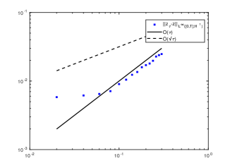
Figure 2: Errors for the approximation of the parameterized solution (62) using the local minimization scheme.

4.2 Locally uniformly convex energy

We next give a one-dimensional example, in which the energy is not globally uniformly convex. In particular, the energetic solution will no longer be continuous in time, which is seen in Figure 3. However, the parametrized solution is still Lipschitz-continuous and moreover remains in a region, where the energy is uniformly convex, see Figure 3. For this example, we set $\mathcal{Z}=\mathcal{V}=\mathcal{X}=\mathbb{R}$ as well as:

(63) $$\mathcal{R}(v)=\lvert v\rvert\quad\text{and}\quad\mathcal{I}(t,z)=\frac{1}{2}z^{2}+\mathcal{F}(z)-\ell(t)z$$

with

$$\mathcal{F}(z)=\left\{\begin{array}[]{rc}2z^{3}-5/2\,z^{2}+1&,z\geq 0\\ -2z^{3}-5/2\,z^{2}+1&,z<0\end{array}\right.\quad\text{and}\quad\ell(t)=-1/2(t-3/2)^{2}+3/2.$$

For $z_{0}=-2/3$, a (differential) solution to (RIS) with (63) reads

(64) $$z(t)=\left\{\begin{array}[]{rl}-2/3&,t\in[0,1/2)\\ -\frac{1}{3}(1+1/2\sqrt{1+3(t-3/2)^{2}})&,t\in[1/2,2)\\ -1/2&,t\in[2,3]\end{array}\right.$$

By direct calculations, one verifies that $z$ indeed stays in a region, where $\mathcal{I}$ is uniformly convex. Thus, from the analysis in Section 3, we expect the error in the approximation to be of order $\mathcal{O}(\tau)$, which can be nicely observed in the Figure 3 below.

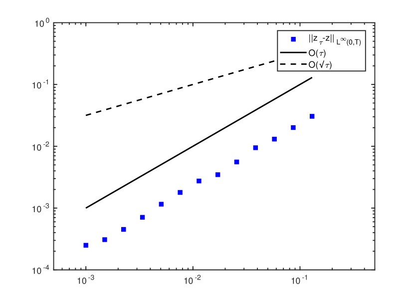
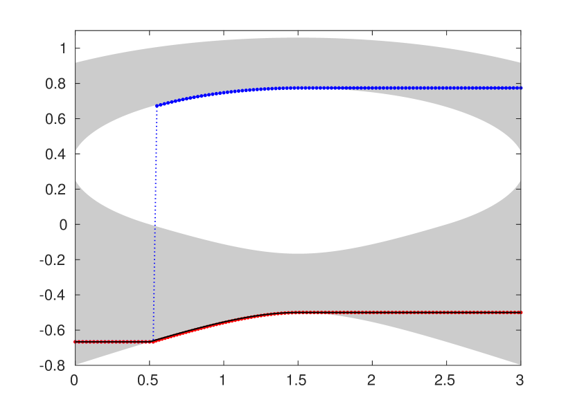
Figure 3: Left: Errors for the approximation of a parametrized solution using the local minimization scheme depending on the stepsize $\tau$; Right: Corresponding differential solution (black) as well as the numerical approximations using the global (blue) and the local iterated minimization scheme (red) as functions of the time $t$.

Appendix A Estimation of the error measure $\gamma$

In the proofs of Theorem 3.15 and Theorem 3.29, we use an adapted version of an estimate that is part of the proof of uniqueness for solutions of RIS from [15]. For convenience of the reader, we present this adapted version here. Therefor let $z_{1},z_{2}\in W^{1,\infty}([0,T];\mathcal{Z})$ and again $\gamma(t):=\langle D_{z}\mathcal{I}(t,z_{1}(t))-D_{z}\mathcal{I}(t,z_{2}(t)),z_{1}(t)-z_{2}(t)\rangle_{\mathcal{Z}^{\ast},\mathcal{Z}}$. First of all we calculate

$$\dot{\gamma}(t) =\langle D^{2}_{z}\mathcal{I}(t,z_{1}(t))[z_{1}(t)-z_{2}(t)],z_{1}^{\prime}(t)\rangle_{\mathcal{Z}^{\ast},\mathcal{Z}}-\langle D^{2}_{z}\mathcal{I}(t,z_{2}(t))[z_{1}(t)-z_{2}(t)],z_{2}^{\prime}(t)\rangle_{\mathcal{Z}^{\ast},\mathcal{Z}}$$

$$\quad+\langle D_{z}\mathcal{I}(t,z_{1}(t))-D_{z}\mathcal{I}(t,z_{2}(t)),z_{1}^{\prime}(t)-z_{2}^{\prime}(t)\rangle_{\mathcal{Z}^{\ast},\mathcal{Z}},$$

where we used the symmetry of $D_{z}^{2}\mathcal{I}$. Note that, due to the special structure of $\mathcal{I}$, the partial derivative w.r.t. $t$ is equal to zero. Rearranging terms, we arrive at

$$\dot{\gamma}(t) =\langle D^{2}_{z}\mathcal{I}(t,z_{1}(t))[z_{1}(t)-z_{2}(t)]+D_{z}\mathcal{I}(t,z_{2}(t))-D_{z}\mathcal{I}(t,z_{1}(t)),z_{1}^{\prime}(t)\rangle_{\mathcal{Z}^{\ast},\mathcal{Z}}$$

$$\quad-\langle D^{2}_{z}\mathcal{I}(t,z_{2}(t))[z_{1}(t)-z_{2}(t)]+D_{z}\mathcal{I}(t,z_{1}(t))-D_{z}\mathcal{I}(t,z_{2}(t)),z_{2}^{\prime}(t)\rangle_{\mathcal{Z}^{\ast},\mathcal{Z}}$$

$$\quad+2\langle D_{z}\mathcal{I}(t,z_{1}(t))-D_{z}\mathcal{I}(t,z_{2}(t)),z_{1}^{\prime}(t)-z_{2}^{\prime}(t)\rangle_{\mathcal{Z}^{\ast},\mathcal{Z}}$$

Now, due to $z_{1},z_{2}\in W^{1,\infty}([0,T];\mathcal{Z})$ and the regularity on $\mathcal{I}(t,\cdot)$ (see (4)), we find that

$$\dot{\gamma}(t) \leq C\lVert z_{1}(t)-z_{2}(t)\rVert_{\mathcal{Z}}^{2}\lVert z_{1}^{\prime}(t)\rVert_{\mathcal{Z}}+C\lVert z_{1}(t)-z_{2}(t)\rVert_{\mathcal{Z}}^{2}\lVert z_{2}^{\prime}(t)\rVert_{\mathcal{Z}}$$

$$\quad+2\langle D_{z}\mathcal{I}(t,z_{1}(t))-D_{z}\mathcal{I}(t,z_{2}(t)),z_{1}^{\prime}(t)-z_{2}^{\prime}(t)\rangle_{\mathcal{Z}^{\ast},\mathcal{Z}}$$

$$\leq C\lVert z_{1}(t)-z_{2}(t)\rVert_{\mathcal{Z}}^{2}+2\langle D_{z}\mathcal{I}(t,z_{1}(t))-D_{z}\mathcal{I}(t,z_{2}(t)),z_{1}^{\prime}(t)-z_{2}^{\prime}(t)\rangle_{\mathcal{Z}^{\ast},\mathcal{Z}}$$

which is the desired estimate.

Appendix B Existence and Uniqueness of differential solutions

The statements of Theorem 3.15 and Theorem 3.29 each refer to the unique differential solution of (RIS), which exists due to [15, Thm. 7.4]. However, in [15], the energy functional is assumed to be slightly more regular than as in (4). For completeness, we therefor bring together the necessary results from the literature to obtain the existence and uniqueness of differential solutions in our setting.

Theorem B.1.

Let $\mathcal{I}$ fulfill Assumption 3, i.e., it is $\kappa$-uniformly convex . Then there exists a unique differential solution $z\in W^{1,\infty}(0,T;\mathcal{Z})$, i.e. it holds

(65) $$0\in\partial\mathcal{R}(z^{\prime}(t))+D_{z}\mathcal{I}(t,z(t))\quad\text{f.a.a.\ }t\in[0,T].$$

Proof B.2.

First of all, the existence of a differential solution satisfying $z\in W^{1,\infty}(0,T;\mathcal{Z})$ follows from [14, Cor. 3.4.6(i)] combined with [14, Cor. 3.1.2]. Moreover, since $\mathcal{I}(t,\cdot)$ is uniform convex, every differential solution has to fulfill $z\in W^{1,\infty}(0,T;\mathcal{Z})$ as a result of [14, Thm. 3.4.4] (with $\alpha=2$, $\beta=1$) and [14, Cor. 3.4.6(i)]. Now, let $z_{1},z_{2}\in W^{1,\infty}(0,T;\mathcal{Z})$ be two differential solutions. We again define $\gamma(t):=\langle D_{z}\mathcal{I}(t,z_{1}(t))-D_{z}\mathcal{I}(t,z_{2}(t)),z_{1}(t)-z_{2}(t)\rangle$. Since $z^{\prime}\in L^{1}([0,T];\mathcal{Z})$, (65) is equivalent to

(66) $$\mathcal{R}(z^{\prime}(t))\geq\mathcal{R}(v)+\langle-D_{z}\mathcal{I}(t,z(t)),v-z^{\prime}(t)\rangle_{\mathcal{Z}^{\ast},\mathcal{Z}}\quad\forall v\in\mathcal{Z}.$$

Testing this variational inequality for $z_{1}$ with $z_{2}$ and vice versa and adding up the resulting inequalities, we obtain

$$0\geq\langle D_{z}\mathcal{I}(t,z_{1}(t))-D_{z}\mathcal{I}(t,z_{2}(t)),z_{1}^{\prime}(t)-z_{2}^{\prime}(t)\rangle_{\mathcal{Z}^{\ast},\mathcal{Z}}.$$

Exploiting the estimate from Section A, we thus have $\dot{\gamma}(t)\leq C\lVert z_{1}(t)-z_{2}(t)\rVert_{\mathcal{Z}}^{2}$. The $\kappa$-uniform convexity of $\mathcal{I}$ implies $\gamma(t)\geq\kappa\lVert z_{1}(t)-z_{2}(t)\rVert_{\mathcal{Z}}^{2}$, so that $\dot{\gamma}(t)\leq C\gamma(t)$ and we obtain the uniqueness result by applying the Gronwall-Lemma.

References

- [1] J. Alberty and C. Carstensen, Numerical analysis of time-depending primal elastoplasticity with hardening, SIAM Journal on Numerical Analysis, 37 (2000), pp. 1271–1294.
- [2] M. Artina, F. Cagnetti, M. Fornasier, and F. Solombrino, Linearly constrained evolutions of critical points and an application to cohesive fractures., Math. Models Methods Appl. Sci., 27 (2017), pp. 231–290, https://doi.org/10.1142/S0218202517500014.
- [3] S. Bartels, Quasi-optimal error estimates for implicit discretizations of rate-independent evolutions, SIAM Journal on Numerical Analysis, 52 (2014), pp. 708–716.
- [4] M. A. Efendiev and A. Mielke, On the rate-independent limit of systems with dry friction and small viscosity, Journal of Convex Analysis, 13 (2006), pp. 151–167.
- [5] W. Han and B. Reddy, Plasticity, Springer, New York, 1999.
- [6] D. Knees, Convergence analysis in time-discretization schemes for rate-independent systems. submitted to ESAIM:COCV, 2017, https://arxiv.org/pdf/1712.06851.pdf.
- [7] D. Knees and A. Schröder, Computational aspects of quasi-static crack propagation, Discrete and Continuous Dynamical Systems. Series S, 6 (2013), pp. 63–99, https://doi.org/10.3934/dcdss.2013.6.63.
- [8] C. Meyer and M. Sievers, Finite element discretization of local minimization schemes for rate-independent evolutions, Calcolo, 56 (2019), https://doi.org/10.1007/s10092-018-0301-4.
- [9] A. Mielke, Chapter 6 evolution of rate-independent systems, Handbook of Differential Equations, Evolutionary Equations, 2 (2006).
- [10] A. Mielke, Differential, energetic, and metric formulations for rate-independent processes, Nonlinear PDE’s and Applications, 2028 (2011), pp. 87–167.
- [11] A. Mielke, L. Paoli, A. Petrov, and U. Stefanelli, Error estimates for space-time discretizations of a rate-independent variational inequality, SIAM Journal on Numerical Analysis, 48 (2010), pp. 1625–1646.
- [12] A. Mielke, R. Rossi, and G. Savaré, BV solutions and viscosity approximations of rate-independent systems, ESAIM. Control, Optimisation and Calculus of Variations, 18 (2012), pp. 36–80, https://doi.org/10.1051/cocv/2010054.
- [13] A. Mielke, R. Rossi, and G. Savaré, Balanced viscosity (BV) solutions to infinite-dimensional rate-independent systems., J. Eur. Math. Soc. (JEMS), 18 (2016), pp. 2107–2165, https://doi.org/10.4171/JEMS/639.
- [14] A. Mielke and T. Roubíc̆ek, Rate-Independent Systems: Theory and Application, Springer-Verlag, New York, 2015.
- [15] A. Mielke and F. Theil, On rate-independent hysteresis models, NoDEA: Nonlinear Differential Equations and Applications, 11 (2004), pp. 151–189.
- [16] M. Negri, Quasi-static rate-independent evolutions: characterization, existence, approximation and application to fracture mechanics, ESAIM Control Optim. Calc. Var., 20 (2014), pp. 983–1008, https://doi.org/10.1051/cocv/2014004.
- [17] F. Rindler, S. Schwarzacher, and E. Süli, Regularity and approximation of strong solutions to rate-independent systems, Mathematical Models and Methods in Applied Sciences, 27 (2017), pp. 2511–2556, https://doi.org/10.1142/S0218202517500518.