Prior Activation Distribution (PAD): A Versatile Representation to Utilize DNN Hidden Units

Abstract

In this paper, we introduce the concept of Prior Activation Distribution (PAD) as a versatile and general technique to capture the typical activation patterns of hidden layer units of a Deep Neural Network used for classification tasks. We show that the combined neural activations of such a hidden layer have class-specific distributional properties, and then define multiple statistical measures to compute how far a test sample’s activations deviate from such distributions. Using a variety of benchmark datasets (including MNIST, CIFAR10, Fashion-MNIST & notMNIST), we show how such PAD-based measures can be used, independent of any training technique, to (a) derive fine-grained uncertainty estimates for inferences; (b) provide inferencing accuracy competitive with alternatives that require execution of the full pipeline, and (c) reliably isolate out-of-distribution test samples.

1 Introduction

Deep Neural Networks (DNNs) [27] have rapidly become an indispensable mechanism for implementing machine intelligence for a variety of tasks, such as medical image analysis [29], chatbots for conversational interactions [20] and navigation of autonomous vehicles & robots [39, 40, 10]. DNNs represent state-of-the-art techniques for multi-class classification problems, which conventionally use the point estimates of the final softmax layer to identify the class with the highest confidence value.

DNNs are still largely viewed as “black box" models that generate inferences—a significant amount of ongoing research focuses on improving their final-layer accuracy, often by increasing the depth of the inferencing pipeline (e.g., Resnet [17] with 152 layers). With a few notable exceptions (e.g., [2, 52, 6]), researchers have typically not devoted much systematic attention to characterizing or exploiting the activation values of intermediate, hidden layers. In this work, inspired by the work of Alain & Bengio [2] in understanding hidden DNN layers, we “unpack” this black box and propose the novel concept of Prior Activation Distribution (PAD) as a fundamental construct for characterizing DNNs. PAD specifically focuses on the activation values associated with hidden units (e.g., dense neurons, flattened convolutional layers, pooling layer values), and uses aggregated, statistical properties of such activation values as a formal mechanism to tackle a variety of DNN-related problems.

We initially developed the PAD construct to quantify the predictive uncertainty associated with DNN inferences. It is known that the confidence values of the softmax layer alone do not capture the uncertainty of the underlying inferencing process [36, 12, 24]. Recently proposed Bayesian Deep Learning (BDL) approaches [32, 31] can model such DNN uncertainty in a more theoretically-grounded manner, but impose significant computational complexity in both training and inference [12]. Moreover, softmax-based inferences require the execution of the entire DNN pipeline, which may impose high latency when executed on resource-limited embedded platforms. We shall show that PAD serves as a versatile, computationally-inexpensive way to quantify such uncertainty: PAD makes no assumption on the training mechanism and can be applied independent of the choice of regularization techniques (e.g., dropout,batch normalization, data augmentation). In addition, we provide evidence that (a) PAD-based uncertainty measures may enable more reliable filtering of out-of-distribution (OOD) data without compromising the base classification accuracy, and (b) the use of PADs may enable us to achieve competitive accuracy while only partially executing the DNN pipeline.

1.1 Hypothesis and Contribution

Our hypothesis is that, given any existing (trained) DNN model, the activation values of each hidden unit of a DNN contain latent information, that makes it more or less likely to be generated by a member of a specific class. By collecting the activation values from all training instances of a specific class, we can then create an appropriate, per-class, representation of the typical range, or distribution of each neuron’s values. When making inferences (on a test sample), we posit that the larger the deviation of a hidden unit’s activation value from this typical range, for a specific class, the lower the likelihood that the sample belongs to this class. By aggregating such deviation scores (through appropriate statistical features) across all the neurons in an hidden layer, we believe that we can better quantify the test sample’s likelihood of belonging to this class. Overall, PADs allow us to analyze DNNs by understanding the behavior of neurons in hidden layers, which we believe represents a step towards the goals of making deep learning models more uncertainty-aware, less computationally complex and more interpretable. PADs also provide attestation to our belief that exploiting the behavior of hidden layers can help build richer models of DNN behavior than possible solely from output layer observations.

Key Contributions: We highlight the following key contributions:

• We introduce the novel concept of Prior Activation Distribution (PAD), a simple technique to model hidden-unit activations of a DNN in multi-class classification problems. Further, we empirically demonstrate that PADs can be utilized to model different types of layers, regardless of the model architecture or regularization techniques used. We also develop statistical measures, over PAD values, that help represent such hidden unit behavior.

• We empirically demonstrate that PADs can capture and quantify the "Predictive Uncertainty" associated with a classification output. PAD-based uncertainty measures corrrespond closely to alternative, more complex models for uncertainty computation.

• We show that, by using additional PAD-based features in conjunction with conventional output confidence scores, DNN classifiers can robustly identify and discard out-of-distribution (OOD) test samples, without sacrificing the ability to reliably classify in-distribution samples. We also provide early empirical evidence that PADs can be leveraged on to provide high classification accuracy, without executing the entirety of a DNN pipeline.

2 Proposed Approach

2.1 Formulating the Hidden Units of Hidden Layers

Let’s consider a trained DNN model G for a |C|-class classification problem, which has been trained using training data $\textbf{X}_{train}=\{\textbf{x}_{1},\textbf{x}_{2},..,\textbf{x}_{m}\}$ and training labels $\textbf{Y}_{train}=\{\textbf{y}_{1},\textbf{y}_{2},..,\textbf{y}_{m}\}$ where $m$ is the training dataset size and $C$ denotes the set of class labels. Let $\textbf{Y}_{train}^{out}=\{\textbf{y}_{1}^{out},\textbf{y}_{2}^{out},..,\textbf{y}_{m}^{out}\}$ be the set of output labels, when evaluated on the $\textbf{X}_{train}$ it self. The convention is to calculate training accuracy using the instances where $\textbf{y}_{i}^{out}=\textbf{y}_{i}$ where $\textbf{y}_{i}^{out}\in\textbf{Y}_{train}^{out}$, $\textbf{y}_{i}\in\textbf{Y}_{train}$ and $i\in[1,\textbf{m}]$.

Consider a G, with a set of layers $\textbf{L}=\{\textbf{l}_{1},\textbf{l}_{2},..,\textbf{l}_{p}\}$, such that the number of hidden units in each layer be denoted by the set $\textbf{S}=\{\textbf{s}_{1},\textbf{s}_{2},..,\textbf{s}_{p}\}$, where $p$ = number of hidden layers. We can represent activation of a hidden unit $\textbf{a}_{i}$ in a particular layer $\textbf{l}_{j}$ as $\alpha_{\textbf{a}_{i}}^{\textbf{l}_{j}}$ where $\textbf{l}_{j}\in\textbf{L}$, $\textbf{a}_{i}\in[1,\textbf{s}_{j}]$, $\textbf{s}_{j}\in\textbf{S}$. Here, $\textbf{s}_{j}$ represents the number of hidden units in the layer $\textbf{l}_{j}$. To avoid ambiguity, we positionally index layers from beginning to the end (thus $\textbf{l}_{1}$ represents the input layer), and the hidden-units from top to bottom (thus $a_{1}^{\textbf{l}_{j}}$ represents the top-most neuron in the $j^{th}$ layer).

Extending this terminology, we define $\alpha_{\textbf{a}_{j},\textbf{c}_{t}}^{\textbf{l}_{i},\textbf{x}_{e}}$ where activation of a hidden unit with (1) positional index $\textbf{a}_{j}\in[1,\textbf{s}_{j}]$ in layer $\textbf{l}_{i}\in\textbf{L}$, when (2) the input to G is $\textbf{x}_{e}\in\textbf{X}_{train}$, and (3) output of the network is correct, and (4) it belongs to class $\textbf{c}_{t}\in\textbf{C}$. Here $\textbf{C}=\{\textbf{c}_{1},\textbf{c}_{2},..,\textbf{c}_{n}\}$ is the set of classification outputs. When $\textbf{X}_{train}$ is used, with 1 stochastic forward pass of each $\textbf{x}_{e}\in\textbf{X}_{train}$ through model G, using the above definitions, we are able to obtain a distribution of activations, for each class, for each hidden unit. We refer to this set of distributions, as the Prior Activation Distribution (PAD).

We make the following two important observations: (a) Independent of Learning Technique: The PAD distributions are derived merely by passing the elements of the training dataset through an already trained DNN—the definition of PAD is thus agnostic to the choice of training methods and parameters; (b) Utilizes Correct Classifications only: Only training instances that are correctly classified contribute to the PAD model. This makes intuitive sense: PAD is used to represent the distribution of neural behavior observed, per class, only when the model is accurate.

For a hidden unit in the positional index of a in layer l, PAD can be denoted using the notation;

$$\textbf{PAD}=\{\textbf{D}(\mu_{a,c_{1}}^{l},\sigma_{a,c_{1}}^{l}),\textbf{D}(\mu_{a,c_{2}}^{l},\sigma_{a,c_{2}}^{l}),...,\textbf{D}(\mu_{a,c_{n}}^{l},\sigma_{a,c_{n}}^{l})\}$$ (1)

$$\mu_{a,c_{t}}^{l}=\frac{\sum\alpha_{a,c_{t}}^{l,x_{e}}}{\text{count}_{c_{t}}}\;\;\mbox{and}\;\sigma_{a,c_{t}}^{l}=\sqrt{\frac{\sum(\alpha_{a,c_{t}}^{l,x_{e}}-\mu_{a,c_{t}}^{l})^{2}}{\text{count}_{c_{t}}}}\text{ where }\textbf{c}_{t}\in\textbf{C}\text{, }\textbf{x}_{e}\in\textbf{X}_{train}$$ (2)

In this definition, D denotes any arbitrary empirical distribution, $count_{\textbf{c}_{t}}$ is the number of accurate inferences for $\textbf{x}_{e}$ which outputs a particular class $\textbf{c}_{t}$. As suggested by our hypothesis, the above definitions allow us to model each hidden unit as a PAD which consists of several distributions, each of which characterize how the hidden-unit activations should behave to produce a particular classification ($\textbf{c}_{t}\in\textbf{C}$). Note also that we make no distributional assumptions (e.g., Gaussian, often used in prior work [12, 14, 19, 37]) on D; in Section 3.1, we shall see that these values are, in fact, quite arbitrary.

2.2 Inference Using PADs: KL-divergence Z-Score metrics

We now describe how statistical properties of such distributions are used to evaluate the ‘fit to a specific class’ of a test sample during the inferencing phase. After choosing a particular layer l which we want to model with PADs, we obtain PADs for all hidden-units in l using the training dataset, denoted by $\textbf{priors}_{l}=\{\textbf{PAD}_{1},\textbf{PAD}_{2},...,\textbf{PAD}_{s}\}$. During the inferencing process, the test sample $\textbf{input}_{test}$ is passed through the DNN and generates a set of $s_{l}$ activation values (one for each hidden unit), in addition to the output prediction (at the final softmax layer) by the DNN. Let us denote these activation values layer l with s hidden units as $\textbf{activations}_{test}=\{\gamma_{1},\gamma_{2},..,\gamma_{s}\}$. We then propose the following 2 representative statistical features to capture the similarity (or divergence) between the activation firings represented by PAD and those resulting from the test instance: (a) the KL-score feature looks at the activation values across all hidden units of a layer jointly, while (b) the Z-score feature first measures per-hidden unit divergence in activation values before aggregating across all hidden units.

2.2.1 KL-Score Metric

At a high-level, the KL-Score considers the set of individual activation values of a layer as a whole–i.e., as a $s$ dimensional vector, and compares the test-instance vector against each of the $|C|$ PAD-based vectors. More specifically, for a layer l with s nodes, the PAD vector for a class $c_{t}$ consists of $s$ elements, where the $a^{th}$ element is obtained by taking the mean value of the activation values $\mu_{a,c_{t}}^{l}$. The distance between the test instance and class $c_{t}$ is computed by the KL-divergence of the normalized values of $\textbf{activations}_{test}$ and the activation vector for class $c_{t}$. In this fashion, one can compute the overall KL-divergence vector $klscores^{l}$, whose elements consist of the KL-divergence measure for each of the $n=|C|$ classes–i.e., $\textbf{klscores}^{l}=\{klscore_{c_{1}},klscore_{c_{2}},....,klscore_{c_{n}}\}.$

Given this formulation, the higher the KL-score, the lower the likelihood of a test instance belong to that class. Accordingly, to classify the test sample using just the KL-score values at hidden layer $l$, we would generate an output corresponding to $\min(\textbf{klscores}^{l})$.

2.2.2 Z-score Metric

This approach first looks at each (hidden,class) individually and computes a Z-score, representing the degree to which the test sample’s activation value can be considered an outlier, given the representative mean ($\mu_{a,c_{t}}^{l}$) and standard deviation ($\sigma_{a,c_{t}}^{l}$). When $n=|C|$, this pseudoZ-score, across all classes, but for neuron $a$ in hidden layer $l$, is first computed as: $\textbf{zscores}_{\textbf{a}}^{\textbf{l}}=\{\frac{\gamma_{a}-\mu_{a,c_{1}}^{l}}{\sigma_{a,c_{1}}^{l}},\frac{\gamma_{a}-\mu_{a,c_{2}}^{l}}{\sigma_{a,c_{2}}^{l}},....,\frac{\gamma_{a}-\mu_{a,c_{n}}^{l}}{\sigma_{a,c_{n}}^{l}}\}.$

Subsequently, the Z-score $zscores^{l}$, across all the $s_{l}$ neurons in layer $l$, is computed as the mean of these $s_{l}$ distinct values, defined as:

$$\begin{split}\textbf{zscores}^{\textbf{l}}&=\{\frac{\sum_{a=1}^{s}\frac{\gamma_{a}-\mu_{a,c_{1}}^{l}}{\sigma_{a,c_{1}}^{l}}}{s},\frac{\sum_{a=1}^{s}\frac{\gamma_{a}-\mu_{a,c_{1}}^{l}}{\sigma_{a,c_{2}}^{l}}}{s},....,\frac{\sum_{a=1}^{s}\frac{\gamma_{a}-\mu_{a,c_{1}}^{l}}{\sigma_{a,c_{n}}^{l}}}{s}\}\\ &=\{zscore_{c_{1}},zscore_{c_{2}},....,zscore_{c_{n}}\}\end{split}$$ (3)

Given this formulation, the higher the Z-score, the lower the likelihood of a test instance belonging to that class. Accordingly, to classify the test sample using the observed activations at hidden layer $l$, we would generate an output corresponding to $\min(\textbf{zscores}^{\textbf{l}})$.

3 Preliminary Analysis

Dataset Model Summary Training Testing Split Regularization techniques Optimizer Reference MNIST C32, D128, D10 60000-10000 Dropout adam MA1 MNIST C64, C128, D128, D10 (Modified LeNet-5 [28]) 60000-10000 Dropout adam MA2 MNIST C32, C64, D128, D10 [9] 60000-10000 Dropout adam MA3 CIFAR10 C32, C32, C64, C64, D512, D10 [8] 50000-10000 Dropout adam CA1 CIFAR10 Modified All Convolutional Net [44, 23] 50000-10000 Batch Normalization, Dropout RMS(learning rate = 0.01, decay = 1e-6) CA2 CIFAR10 All Convolutional Net [44] 50000-10000 Data Augmentation SGD(learning rate = 0.01, decay = 1e-6) CA3 Fashion-MNIST C64, C32, D256, D10 [33] 60000-10000 Dropout adam FMA1 NotMNIST - NA-100000 - - NM1 Modified-MNIST - NA-10000 - - MM1

Table 1: Summary of the datasets and model architectures. The notation uses C, D to represent Conv2D & Dense units respectively, while the subsequent number specifies the number of hidden-units:e.g., D128 represents a layer with 128 dense neurons.

In this section and section 4, we extensively analyze the properties of PAD (and the related KL and Z-score features), using multiple benchmark classification datasets: MNIST [28], CIFAR10 [22], Fashion-MNIST [50], notMNIST [5], Modified-MNIST datasets. All the experiments were implemented and evaluated using Python [47] with Keras library [7] with a Tensorflow [11] backend. All the model configurations we used are summarized in Table 1.

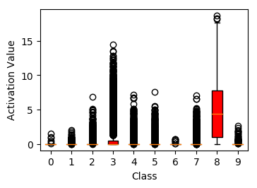
(a) Hidden-unit #1

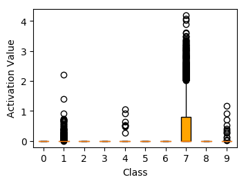
(b) Hidden-unit #65

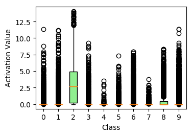
(c) Hidden-unit #128

Figure 1: Examples for activation distributions of hidden-units of a DNN trained for MNIST dataset. The hidden-units here are from a layer with 128 neurons & numbering was done from top to bottom.

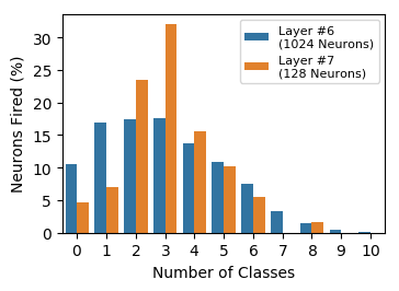
Figure 2: Histogram of number of classes against fired neurons percentage

3.1 Behavior of Hidden-Layer Activations of DNNs

We carried out several preliminary experiments to understand the behavior of hidden layer activations. We will use the following example to illustrate our findings. We trained a DNN for MNIST dataset with configuration MA3 (2) (a model with 1024 flattened values from Conv2D layers – layer 6, 128 dense neurons – layer 7 with ReLU activations). Figure 2 provides boxplot [21] based visualizations (one for each of the 10 classes) of some representative dense neurons in layer 7, and Figure 2 provides a histogram plot of the number of hidden units that fire for distinct classes (for both layer 6 & 7).

We make the following observations. hidden unit number 1 (Figure 1(a)) generates a wide range of activation values for the $9^{th}$ class, but has activation values very close to 0 for the $1^{st}$, $2^{nd}$ $7^{th}$ & $10^{th}$ classes. On a similar note, hidden-unit 128 (the middle neuron in th layer, illustrated in Figure 1(c)) shows a unique pattern for the activation value distribution for the $3^{rd}$ class. On the other hand, hidden unit 65 (Figure 1(b)) effectively does not generate non-zero activation values for 6 output classes. From similar analysis performed with both MNIST and CIFAR10 datasets, we observe that: (a) hidden unit activations typically possess a unique distributional pattern for one or more classes and (b) the distributions are not necessarily normal. These unique patterns might help in both discriminating among classes and in quantifying uncertainty–e.g., if the activation value of hidden-unit 1 for an unknown test instance (that has been declared to be the $9^{th}$ class by the softmax output) is, say, 15.0 rather than 5.1 (closer to the mean of $9^{th}$ class), the DNN is likely to be more uncertain of this classification. Our plots clearly show that distributions are not typically normal. In addition, Figure 2 plots the histogram (percentage) of hidden units, as a function of the number of distinct classes that activate each hidden unit at least once. We see that, across both layers 6 and 7, the dominant majority of hidden units are fired by three or fewer of the 10 classes. This result provides further evidence that most hidden units have distinct class-dependent activation patterns, lending further credence to our exploration of PADs as a means for identifying class labels for test samples.

3.2 Characterizing KL-score and Z-Score

In this section, we evaluate the characteristics of KL-divergence and Z-score based values obtained for several images from MNIST and CIFAR10 datasets using MA3 & CA1 configurations (Table 1 & 4), respectively. Table 2 shows different KL and Z-score values, as well as the output of the softmax layer, the classes corresponding to the minimum KL and Z-scores and the ground truth, for 4 different representative images (2 for MNIST, 2 for CIFAR10) illustrated in Figure 4.

In the MNIST sample (ground truth=6) in Figure 3(a), the minimum KL score (1.073) and Z-score (0.594) for this sample (plotted in Table 2) correspond to the correct class “6". In this case, the softmax output, the minimum KL-score and the minimum Z-score label all agree and are correct. In contrast, for Figure 3(b), the class with the minimum KL and Z-score is 9 (agreeing with the ground truth), whereas softmax output suggests the class 5. In this case, the PAD-related features provide a correct classification while the output softmax does not. Figure 3(c) depicts an interesting example where the two top softmax output candidates ("ship" with 76.5% confidence and "truck" with 18.8% confidence) are both incorrect. However, the KL and Z-score metrics provide “automobile" (the correct inference) and “truck" respectively. Further, in Figure 3(d), the softmax layer outputs the class "truck" (confidence> 73.1%), whereas the KL and/or Z-scores correctly indicate that the output should be "dog". While we defer the presentation of comprehensive results on overall accuracy till Section 4, the examples presented here do attest to the discriminative potential of PADs.

Example KL-scores Softmax Output min of KL min of Z-scores Ground truth Z-scores Figure 3(a) {2.223, 1.627, 1.653, 1.599, 1.539, 1.364, 1.073, 1.169, 1.181, 1.239} 6 (98%) 6 6 6 {1.987, 1.147, 1.062, 0.975, 0.881, 0.733,0.594, 0.633, 0.636, 0.657} Figure 3(b) {2.445, 2.038, 2.08, 1.566, 1.442, 1.207, 1.269, 1.188, 1.183, 1.125} 5 (78%) 9 9 9 {1.951, 1.321, 1.224, 0.877, 0.702, 0.58, 0.600, 0.567, 0.566, 0.547} Figure 3(c) {2.465, 1.335, 3.798, 3.483, 4.373, 4.006, 3.849, 4.244, 1.396, 1.454} ship (76.5%) automobile truck automobile {1.951, 1.321, 1.224, 0.877, 0.702, 0.58, 0.600, 0.567,0.566,0.547} Figure 3(d) {2.223, 1.627, 1.653, 1.599, 1.539, 1.364, 1.073, 1.169, 1.181, 1.239} truck (73.1%) dog dog dog {1.987, 1.147, 1.062, 0.975, 0.881, 0.733, 0.594, 0.633, 0.636, 0.657}

Table 2: Example figures and KL-score, Z-score characterization

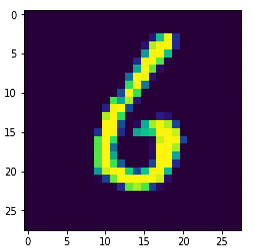
(a) MNIST:
"6"

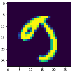
(b) MNIST:
"9"

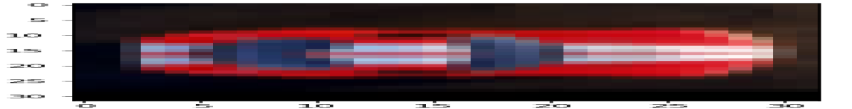
(c) CIFAR10:
"automobile"

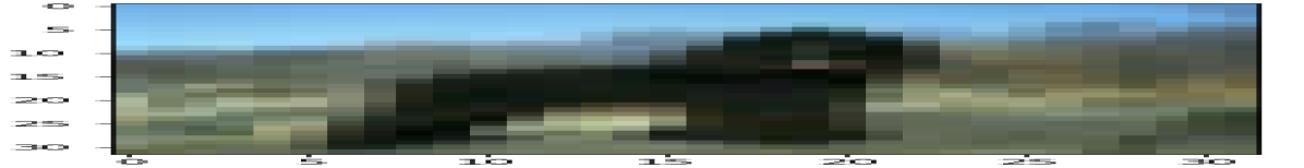
(d) CIFAR10:
"dog"

Figure 3: Examples for PAD characterization

Figure 4: Example from Modified-MNIST dataset

4 Experimental Evaluation of PAD Performance

In this section, we empirically show that PADs can be used for a variety of uses, ranging from uncertainty quantification to ensuring highly accurate inferences.

4.1 Using PADs for Uncertainty Quantification

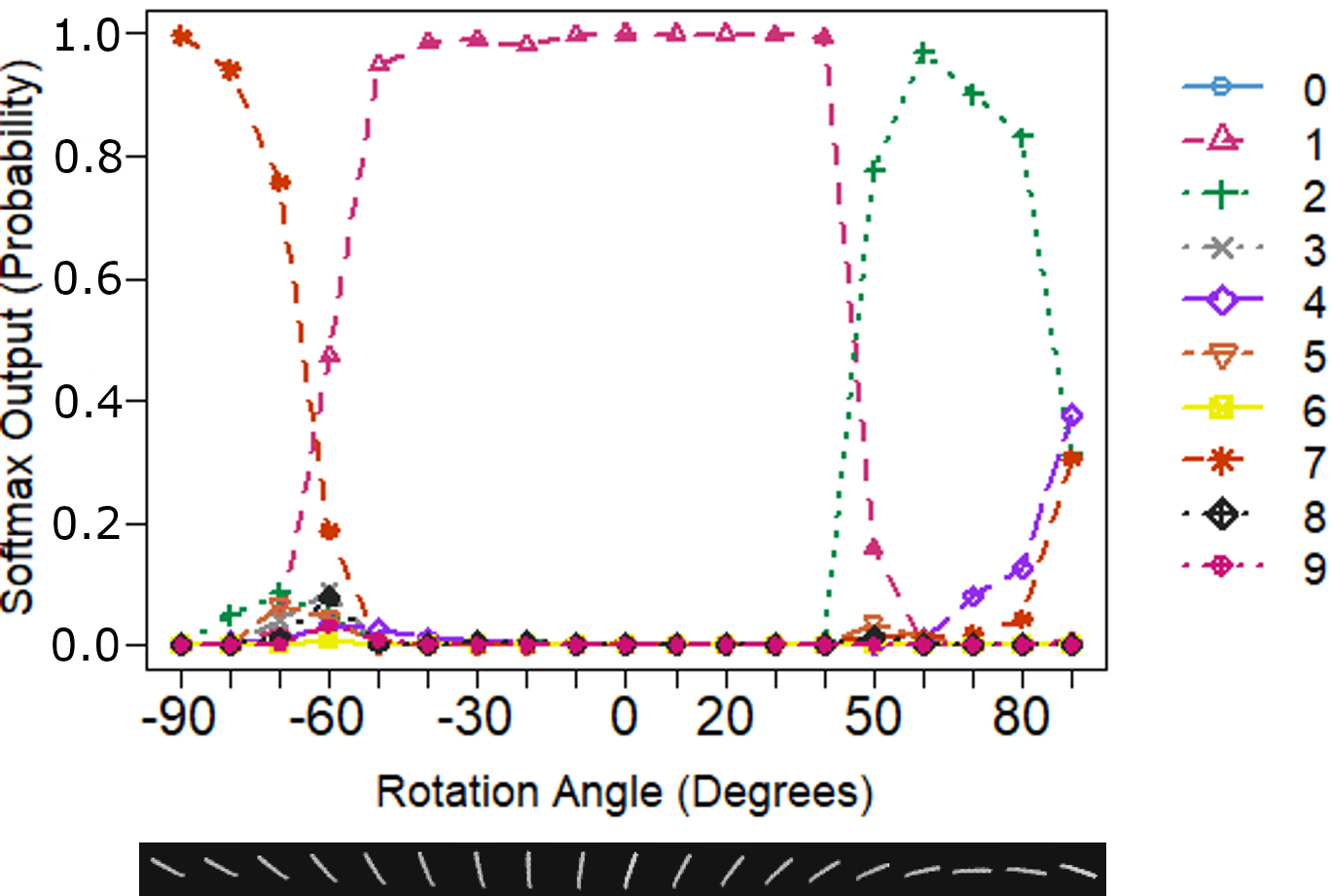
Figure 5: Softmax (MA1 model): Rotational MNIST

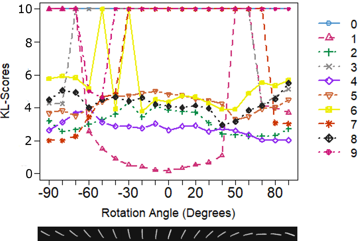
Figure 6: KL-Score (MA1 model): Roational MNIST

	MNIST	CIFAR-5
MC Dropout [14]	99.5 %	84 %
Deep Ensemble [25]	99.3 %	79 %
EDL [43]	99.3 %	83 %
Softmax	99.4 %	80 %
KL	99.1 %	79 %
Z-score	96.3 %	76 %

Table 3: Comparison of classification accuracies for MNIST and CIFAR-5 for uncertainty quantifying techniques using LeNet configuration in [30]

In this section, we observe how uncertainty is quantified using PADs of hidden layer units. Similar to experiments carried out by Gal et. al. [14] and Sensoy et. al.[43], we carried out experiments using PADs (with several configurations) on MNIST images under varying degrees of rotation. Figures 6 and  6 show the softmax outputs and KL-scores obtained using the MA1 model (Table 1), using rotations on an original “1" sample. For rotation angles between (-90^∘,-65^∘), both softmax output and KL-scores suggest that the output is in fact 7. But, the softmax output gives confidence values in excess of 75% (more than 90% for certain angles), which is over-optimistic given that the model was never trained for such images. Similar results were observed in Gal et. al., where they obtain a distribution of softmax outputs using dropout. However, even the dropout-based technique (as well as prior Bayesian approaches) result in higher confidence values. The PAD-based approach (Figure 6), however provides a more conservative picture: while the class “7" does have the lowest KL-score, the KL-scores of other classes (e.g., “2" & “4") are quite similar, indicating that the DNN is not very confident of its inference. Similar results hold for rotation angles between (50^∘,90^∘), where the softmax output continues to have a misleadingly high confidence ($>$75%). However, in the “normal range" of (-40^∘,40^∘), the KL-score for the correct class (“1") is significantly lower than that of other classes, indicating that the DNN has low inferencing uncertainty. In addition, we see that the PAD-based KL-score is able to offer a finer-grained measure for uncertainty, with the KL-score for “1" increasing gradually, even for 5^∘ increments. In contrast, the softmax output remains high ($>$96% for all rotations between (-60^∘,50^∘). Further, Table 3 compares classification accuracies of models and techniques which quantify different types of uncertainty (it should be noted that the purpose of these techniques is not to have high accuracies per se, but to have reliable uncertainty estimates).

4.2 Using PADs for Inference

We now show how the discriminative capabilities of KL-score and Z-score values (illustrated in Section 3.2) can help improve the inferencing process. To compare with the baseline approach (based on the softmax output layer), we consider several alternative PAD-based inferencing strategies which operate on the hidden-layer activation values: KL and Z-score approaches output the class with the lowest KL-Score and Z-score, respectively; EnsAND generates a class label only when all 3 measures (softmax, KL, Z-score) unanimously agree on the same class; while EnsOPT serves as an alternative optimal (oracular) baseline that picks the correct class if at least one of the 3 approaches (softmax, KL, Z-score) is correct.

Table 4 plots the classification accuracy of these approaches (for different datasets and models). We see that PAD-based KL and Z-score accuracy comparable to the softmax baseline, especially when applied to neural activations in the latter (deeper) part of the DNN. Further, an optimal ensemble technique EnsOPT, which smartly combines the PAD and softmax output inferences, can in fact exceed baseline accuracy, at least for the MNIST, CIFAR10 and Fashion-MNIST benchmark datasets. We additionally considered configurations CA2, CA3 and observed that PAD-based accuracy increases as we go deeper in the network –for example, in CA2, Z-score based accuracy was 53.1%, 69.4%, 83.45%, 84.05% for convolutional layers numbered 12,17,20 and 24 respectively. This result is consistent with prior work (Section 5) which demonstrates that deeper layers of a DNN are able to capture more specific features. While we omit results due to space limitations, we also tested PAD-based inferencing using other types of hidden layer–e.g., flattened values in CA2, pooling layers in CA3, etc., as well as when different regularization techniques (e.g., Data Augmentation, Dropout, Batch Normalization) were used. The results are consistent: PAD-based classification provides high accuracy under partial computation in all cases, demonstrating the versatility of this representation.

As a final illustration of using PAD in inferencing, we consider the use of of DNNs in mission-critical scenarios, where we desire that automated DNN classification should have ‘near-100%" accuracy–i.e., it should aggressively refer uncertain test samples to explicit manual verification. (An example would be DNNs used in medical image analysis) There is clearly a tradeoff between coverage (the percentage of samples that the DNN automatically classifies) and accuracy (defined over the covered samples). We compare three alternatives in terms of this tradeoff: (a) baseline, which uses the softmax confidence value to quantify uncertainty and thus invokes manual intervention when this confidence falls below a threshold; (b) KL-score and (c) Z-score, both of which invoke manual intervention when the corresponding metric exceeds a specified threshold. Figure 8 plots the resulting accuracy vs. coverage tradeoff. We see that the KL-score approach is able to explore this tradeoff continuum–e.g., it can ensure over 99.99% accuracy by filtering out around 20% of the test samples for manual inspection. In contrast, while the baseline softmax approach does have high initial accuracy, it cannot easily push the accuracy higher as confidence does not reliably indicate uncertainty.

Reference (Table 1) Layer Accuracy Softmax KL Zscore EnsAND EnsOPT MA1 128-Dense Layer 99.03% 98.40% 98.27% 97.88% 99.34% MA2 128-Dense Layer 99.44% 99.17% 99.04% 98.82% 99.59% MA3 128-Dense Layer 99.56% 99.31% 99.15% 99.08% 99.66% CA1 512-Dense Layer 88.17% 88.11% 88.24% 86.85% 89.63% CA2 2048-Flattened Value Layer ($24^{th}$ Layer) 89.31% 84.11% 84.05% 79.25% 92.95% CA3 Average Pooling Layer 92.75% 89.11% 85.74% 78.31% 94.97% FMA1 256-Dense Layer 91.81% 91.22% 91.32% 89.77% 93.23%

Table 4: Comparison of accuracy for different model architectures and datasets

4.3 Using PADs to identify out-of-distribution data

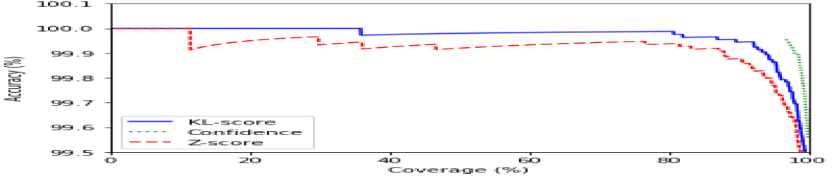
Figure 7: MNIST (MA3):
Coverage vs. Accuracy

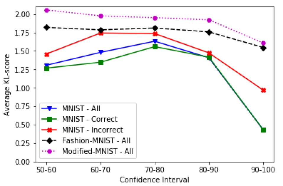
Figure 8: MNIST (MA3):KL-score vs. softmax confidence values, for MNIST & different OOD data. (notMNIST values outside plotted range)

Dataset	S1	S2	S3
notMNIST	100.00%	99.98%	99.98%
Fashion-MNIST	79.77%	97.69%	79.27%
Modified-MNIST	41.74%	98.32%	41.71%
MNIST	00.68%	15.36%	00.89%

Table 5: MA3: Rejection Rate for OOD vs. in-Distribution data for 3 different strategies. (Ideally, OOD rejection rate= 100%.)

Given PAD’s intrinsic characterization of the typical neural activity for each class, we now demonstrate its use in reliably identifying out-of-distribution data (OOD). We used Fashion-MNIST, notMNIST and Modified-MNIST as exemplars of OOD data, injecting their samples into model MA3 (Table 1) that has been trained on the MNIST dataset. For the in-distribution MNIST data, Figure 8 plots the average KL-score values for samples, categorized by the confidence value produced at the output (softmax) layer. Plots are generated separately for the entire MNIST dataset (MNIST-All), as well as the test samples that are correctly or incorrectly classified (MNIST-Correct & MNIST-Incorrect, respectively). We see that even when the classifier is highly confident (confidence values $\in\{90,100\}$%), the KL-score for incorrect samples is more than double (0.97) that of comparable correct samples. Clearly, high KL-scores can help identify incorrect classification attempts.

This trend is further borne out when MA3 is used to classify OOD samples. For both Fashion-MNIST and Modified-MNIST samples, the average KL-score is 3-4 times larger than that obtained for in-distribution samples, even though many OOD samples are associated with high softmax confidence values. To further quantify this, we evaluate 3 different OOD-identification strategies: (i) S1: this filters out samples whose softmax confidence is below a threshold $\alpha$ (=0.95 in the MNIST experiments); (ii) S2: this PAD-based strategy filters out samples whose KL-score exceeds a threshold $\beta$ (=0.65 in our experiments), and (iii) S3: this hybrid strategy filters out only those samples whose $confidence<\alpha\;\mbox{AND}\;KL-score\geq beta$. Table 5 plots the percentage of rejected samples for all 3 strategies. We see that the pure confidence-based S1 strategy is effective only when the data is completely different (notMNIST), but performs poorly (rejection rate $\sim$40%) when the OOD dataset has some similarities (Modified-MNIST). In contrast, strategy S2 can reject the vast majority of OOD samples, but at the cost of a higher rejection rate for in-distribution (MNIST) samples. By combining both predicates, strategy S3 achieves both higher OOD and low in-distribution rejection rates.

5 Related Work

Hidden-Layers of Deep Neural Networks: Researchers have explored the interpretability of Convolutional Neural Networks (CNNs) by analyzing their hidden layers [52, 53]. They have suggested that DNNs tend to learn general features such as Gabon filters or Color blobs in the first few layers, while deeper layers learn more dataset-specific features. In an interesting study, Alain & Bengio [2] discuss the possibility of creating separately trained linear classifiers aka "probes" using parameters of hidden layers. Similar to our study, they reported that linear separability (and thus classification accuracy) increases as we go deeper in the network. However, their approach requires training a separate classifiers. Another study [4] proposes using the alignment of individual hidden units of a CNN to quantify model interpretability. [41] studies class specific information in hidden layers of CNNs using Singular Vector Canonical Correlation Analysis (SVCCA). Our methodology has conceptual overlap with  [6, 41, 2]. However, we believe that PAD provides a novel, generalized construct with multiple uses (unlike [2] – focused purely on classification inference) and defines useful statistical measures on the underlying activation distributions.

Model Pruning: Researchers have proposed different model pruning strategies (e.g., [26, 51, 34, 3]) that utilize various properties of hidden layers –e.g., weight-based pruning of convolutional filters or entire nodes. PAD, on the other hand, models a neuron’s activation values on a per-class basis, and applies statistical aggregation across multiple neurons, as a means to identify class-specific activation patterns.

Uncertainty in DNNs: Bayesian Neural Networks have been discussed thoroughly in literature as a mathematically grounded way of modelling neural network uncertainty [35, 48, 31]. Recently, there has been a shift towards modelling uncertainty using Bayesian Inference [19, 37]. Variational Inference (VI) based Bayesian techniques have been proposed [18, 16] even though their validity has been questioned in subsequent research [42, 38]. Such Bayesian techniques have higher computational complexity, in both training and inference, and are not yet fully supported in mainstream deep learning libraries. Gal et. al. [12, 14] have suggested that Dropout [45] can be utilized to provide Bayesian approximations in DNNs. An alternative technique based on batch normalization was proposed by Teye et. al. [46] which has similar traits to that of [14]. Both these techniques rely on a specific regularization technique (both batch normalization & dropout in CNNs have associated problems [13, 44, 49]). They also require multiple stochastic passes (using the same test sample) to derive an uncertainty measures and are thus not suitable for real-time applications. An ensemble approach for non-Bayesian uncertainty modelling, proposed in [25], requires the use of several DNNs for both training and inferencing. Another interesting work, [43] employs Dempster-Shafer theory (a generalization of bayesian logic [15]) to model uncertainty by adding an additional “uncertainty class" to the output layer–this method requires changes in training (including loss function and logits). In contrast to several of these approaches, PADs requires no modifications to training, does not employ an explicit Bayesian framework and instead uses low dimensional statistics over the activation values of hidden layer units to distinguish between classes.

6 Conclusion

We have proposed a novel and intuitive technique, called PAD, to capture class separability in DNNs using the activation values of hidden layer units. Intuitively, PAD leverages on the collective cross-class discrimination capability of all neurons in a hidden layer, provides greater expressivity than available purely at the output layer. As exemplars of PAD’s utility, we have demonstrated its use for (a) capturing predictive uncertainty in classification; (b) obtaining highly accurate inferences early, without fully executing a DNN; and (c) filtering out out-of-distribution samples.

We believe that PADs provide a promising representation that can form the basis for interesting future work. For example, (a) PADs may need to be modified to be applicable to other tasks (e.g., regression) beyond just classification, and (b) PADs may provide a mechanism for class-aware model compression & pruning (e.g., by selectively discarding neurons that fire across multiple classes and thus are less discriminative).

References

- [1]
- Alain and Bengio [2017] Guillaume Alain and Yoshua Bengio. 2017. Understanding intermediate layers using linear classifier probes. ICLR (Workshop) (2017).
- Anwar et al. [2017] Sajid Anwar, Kyuyeon Hwang, and Wonyong Sung. 2017. Structured Pruning of Deep Convolutional Neural Networks. ACM Journal on Emerging Technologies in Computing Systems (JETC) (2017).
- Bau et al. [2017] David Bau, Bolei Zhou, Aditya Khosla, Aude Oliva, and Antonio Torralba. 2017. Network Dissection: Quantifying Interpretability of Deep Visual Representations. CVPR (2017).
- Bulatov [2011] Yaroslav Bulatov. 2011. notMNIST dataset. (2011). http://yaroslavvb.blogspot.com/2011/09/notmnist-dataset.html
- Chih-Kuan Yeh [2018] Ian E.H. Yen Pradeep Ravikumar Chih-Kuan Yeh, Joon Sik Kim. 2018. Representer Point Selection for Explaining Deep Neural Networks. NIPS (2018).
- Chollet et al. [2015] François Chollet et al. 2015. Keras. https://github.com/fchollet/keras. (2015).
- Chollet et al. [2019a] François Chollet et al. 2019a. CIFAR10 Sample Code - Keras Code Examples GitHub Repository. (2019). https://github.com/keras-team/keras/blob/master/examples/cifar10_cnn.py
- Chollet et al. [2019b] François Chollet et al. 2019b. MNIST Sample Code - Keras Code Examples GitHub Repository. (2019). https://github.com/keras-team/keras/blob/master/examples/mnist_cnn.py
- Duan et al. [2016] Yann Duan, Xi Chen, Rein Houthooft, John Schulman, and Peiter Abbeel. 2016. Benchmarking Deep Reinforcement Learning for Continuous Control. In 33 rd International Conference on Machine Learning (ICML).
- et al [2015] Martín Abadi et al. 2015. TensorFlow: Large-Scale Machine Learning on Heterogeneous Systems. (2015). http://tensorflow.org/ Software available from tensorflow.org.
- Gal [2016] Yarin Gal. 2016. Uncertainty in Deep Learning. PhD Thesis (2016).
- Gal and Ghahramani [2016a] Yarin Gal and Zoubin Ghahramani. 2016a. Bayesian Convolutional Neural Networks with Bernoulli Approximate Variational Inference. ICLR (2016).
- Gal and Ghahramani [2016b] Yarin Gal and Zoubin Ghahramani. 2016b. Dropout as a Bayesian Approximation: Representing Model Uncertainty in Deep Learning. International Conference on Machine Learning (ICML) (2016).
- Gordon and Shortliffe [1984] Jean Gordon and Edward H. Shortliffe. 1984. The Dempster-Shafer Theory of Evidence. Rule-Based Expert Systems: The MYCIN (1984).
- Graves [2011] A Graves. 2011. Practical variational inference for neural networks. NIPS (2011).
- He et al. [2015] Kaiming He, Xiangyu Zhang, Shaoqing Ren, and Jian Sun. 2015. Deep Residual Learning for Image Recognition. arXiv preprint arXiv:1512.03385 (2015).
- Hernandez-Lobato and Adams [2015] J M Hernandez-Lobato and R P Adams. 2015. Probabilistic backpropagation for scalable learning of bayesian neural networks. ICML (2015).
- Herzog and Ostwald [2013] S Herzog and D. Ostwald. 2013. Experimental biology: Sometimes Bayesian statistics are better. Nature 494 (2013).
- H.N.Io and C.B.Lee [2017] H.N.Io and C.B.Lee. 2017. Chatbots and conversational agents: A bibliometric analysis. International Conference on Industrial Engineering and Engineering Management (IEEM) (2017), 215–219. https://doi.org/10.1109/IEEM.2017.8289883
- Hunter [2007] J. D. Hunter. 2007. Matplotlib: A 2D graphics environment. Computing In Science & Engineering 9, 3 (2007), 90–95. https://doi.org/10.1109/MCSE.2007.55
- Krizhevsky [2009] Alex Krizhevsky. 2009. Learning Multiple Layers of Features from Tiny Images. (2009). https://www.cs.toronto.edu/~kriz/cifar.html
- Kumar [2018] Abhijeet Kumar. 2018. Achieving 90% accuracy in Object Recognition Task on CIFAR-10 Dataset with Keras: Convolutional Neural Networks. Applied Machine Learning Blog (2018). http://tiny.cc/c4os6y
- LABS [2019] AiOTA LABS. 2019. Quantifying Accuracy and SoftMax Prediction Confidence For Making Safe and Reliable Deep Neural Network Based AI System. UseJournal (2019).
- Lakshminarayanan et al. [2017] Balaji Lakshminarayanan, Alexander Pritzel, and Charles Blundell. 2017. Simple and Scalable Predictive Uncertainty Estimation using Deep Ensembles. 31st Conference on Neural Information Processing Systems (NIPS) (2017).
- LeCun et al. [1990] Yann LeCun, John S. Denker, and Sara A. Solla. 1990. Optimal Brain Damage. In Advances in Neural Information Processing Systems 2, D. S. Touretzky (Ed.). Morgan-Kaufmann, 598–605. http://papers.nips.cc/paper/250-optimal-brain-damage.pdf
- Lecunn et al. [2015] Yann Lecunn, Yoshua Bengio, and Geoffrey Hinton. 2015. Deep Learning. Nature 521 (2015), 436–444.
- LeCunn et al. [1998] Y. LeCunn, L. Bottou, Y. Bengio, and P. Haffner. 1998. Gradient-based learning applied to document recognition. Proc. IEEE (1998).
- Litjens et al. [2017] Geert Litjens, Thijs Kooi, Babak Ehteshami Bejnordi, Arnaud Arindra Adiyoso Setio, Francesco Ciompi, Mohsen Ghafoorian, Jeroen A.W.M. van der Laak, Bram van Ginneken, and Clara I. Sánchez. 2017. A survey on deep learning in medical image analysis. Medical Image Analysis 42 (2017), 60 – 88. https://doi.org/10.1016/j.media.2017.07.005
- Louizos and Welling [2017] C. Louizos and M. Welling. 2017. Multiplicative normalizing flows for variational bayesian neural networks. ICML (2017).
- MacKay [1992] David JC MacKay. 1992. A practical Bayesian framework for backpropagation networks. Neural computation 4(3) (1992), 448–472.
- MacKay [1995] David JC MacKay. 1995. Probable networks and plausible predictions-a review of practical Bayesian methods for supervised neural networks. Network: Computation in Neural Systems 6(3) (1995), 469–505.
- Maynard-Reid [2018] Margaret Maynard-Reid. 2018. Fashion-MNIST with tf.Keras. (2018).
- Molchanov et al. [2017] Pavlo Molchanov, Stephen Tyree, Tero Karras, Timo Aila, and Jan Kautz. 2017. Pruning Convolutional Neural Networks for Resource Efficient Inference. ICLR (2017).
- Neal [1995] R M. Neal. 1995. Bayesian learning for neural networks. PhD thesis, University of Toronto (1995).
- Nguyen et al. [2015] Anh Nguyen, Jason Yosinski, and Jeff Clune. 2015. Deep Neural Networks are Easily Fooled: High Confidence Predictions for Unrecognizable Images. Conference on Computer Vision and Pattern Recognition (CVPR) (2015).
- Nuzzo [2013] Regina Nuzzo. 2013. Statistical Errors. Nature 506(13) (2013), 150–152.
- Osband et al. [2018] I. Osband, J. Aslanides, and A. Cassirer. 2018. Randomized Prior Functions for Deep Reinforcement Learning. 32nd Conference on Neural Information Processing Systems (NIPS) (2018).
- Pal [2019] Manajit Pal. 2019. Deep Learning for Self-Driving Cars. Towards Data Science (2019).
- Pinto and Gupta [2016] Larrel Pinto and Abhinav Gupta. 2016. Supersizing self-supervision: Learning to grasp from 50K tries and 700 robot hours. IEEE International Conference on Robotics and Automation (ICRA), 3406–3413.
- Raghu et al. [2017] Maithra Raghu, Justin Gilmer, Jason Yosinski, and Jascha Sohl-Dickstein. 2017. SVCCA: Singular Vector Canonical Correlation Analysis for Deep Learning Dynamics and Interpretability. Advances in neural information processing systems(NIPS) (2017).
- Ritter et al. [2018] H. Ritter, A. Botev, and D. Barber. 2018. A scalable laplace approximation for Neural Networks. ICLR (2018).
- Sensoy et al. [2018] Murat Sensoy, Lance Kaplan, and Melih Kandemir. 2018. Evidential Deep Learning to Quantify Classification Uncertainty. 32nd Conference on Neural Information Processing Systems (NeurIPS) (2018).
- Springenberg et al. [2015] Jost Tobias Springenberg, Alexey Dosovitskiy, Thomas Brox, and Martin Riedmiller. 2015. Striving for Simplicity: The All Convolutional Net. ICLR Workshop (2015).
- Srivastava et al. [2014] N. Srivastava, G. Hinton, A. rizhevsky, I. Sutskever, and R. Salakhutdinov. 2014. Dropout: A simple way to prevent neural networks from overfitting. The Journal of Machine Learning Research (2014).
- Teye et al. [2018] Mattias Teye, Hossein Azizpour, and Kevin Smith. 2018. Bayesian Uncertainty Estimation for Batch Normalized Deep Networks. International Conference on Machine Learning (ICML) (2018).
- van Rossum [1995] G. van Rossum. 1995. Python tutorial. Technical Report CS-R9526. Centrum voor Wiskunde en Informatica (CWI), Amsterdam. Software available from python.org.
- Williams [1997] C. K. I. Williams. 1997. Computing with infinite networks. NIPS (1997).
- Xiang Li [2018] Xiaolin Hu Jian Yang Xiang Li, Shuo Chen. 2018. Understanding the Disharmony between Dropout and Batch Normalization by Variance Shift. arXiv:1801.05134 (2018).
- Xiao et al. [2017] Han Xiao, Kashif Rasul, and Roland Vollgraf. 2017. Fashion-MNIST: a Novel Image Dataset for Benchmarking Machine Learning Algorithms. (2017). arXiv:cs.LG/1708.07747
- Yao et al. [2017] Shuochao Yao, Yiran Zhao, Aston Zhang, Lu Su, and Tarek Abdelzaher. 2017. DeepIoT: Compressing Deep Neural Network Structures for Sensing Systems with a Compressor-Critic Framework. SenSys (2017).
- Yosinski et al. [2014] J. Yosinski, J. Clune, Y. Bengio, and H. Lipson. 2014. How transferable are features in deep neural networks? Advances in neural information processing systems(NIPS) (2014), 3320–3328.
- Zeiler and Fergus [2014] M. D. Zeiler and R Fergus. 2014. Visualizing and understanding convolutional networks. European conference on computer vision (ECCV) (2014), 818–833.