Head-Driven Phrase Structure Grammar Parsing on Penn Treebank

Abstract

Head-driven phrase structure grammar (HPSG) enjoys a uniform formalism representing rich contextual syntactic and even semantic meanings. This paper makes the first attempt to formulate a simplified HPSG by integrating constituent and dependency formal representations into head-driven phrase structure. Then two parsing algorithms are respectively proposed for two converted tree representations, division span and joint span. As HPSG encodes both constituent and dependency structure information, the proposed HPSG parsers may be regarded as a sort of joint decoder for both types of structures and thus are evaluated in terms of extracted or converted constituent and dependency parsing trees. Our parser achieves new state-of-the-art performance for both parsing tasks on Penn Treebank (PTB) and Chinese Penn Treebank, verifying the effectiveness of joint learning constituent and dependency structures. In details, we report 96.33 F1 of constituent parsing and 97.20% UAS of dependency parsing on PTB.

1 Introduction

Head-driven phrase structure grammar (HPSG) is a highly lexicalized, constraint-based grammar developed by Pollard and Sag (1994). As opposed to dependency grammar, HPSG is the immediate successor of generalized phrase structure grammar.

HPSG divides language symbols into categories of different types, such as vocabulary, phrases, etc. Each category has different grammar letter information. The complete language symbol which is a complex type feature structure represented by attribute value matrices (AVMs) includes phonological, syntactic, and semantic properties, the valence of the word and interrelationship between various components of the phrase structure.

Meanwhile, the constituent structure of HPSG follows the HEAD FEATURE PRINCIPLE (HFP) Pollard and Sag (1994): “the head value of any headed phrase is structure-shared with the HEAD value of the head daughter. The effect of the HFP is to guarantee that headed phrases really are projections of their head daughter” (p. 34).

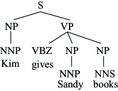
(a) Constituent

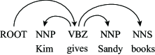
(b) Dependency

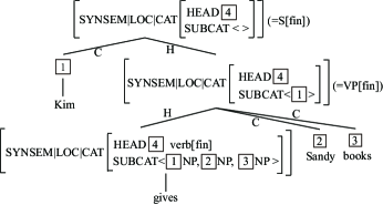
(c) HPSG

Figure 1: Constituent, dependency and HPSG trees.

Constituent and dependency are two typical syntactic structure representation forms, which have been well studied from both linguistic and computational perspective Chomsky (1981); Bresnan et al. (2015). The two formalisms carrying distinguished information have each own strengths that constituent structure is better at disclosing phrasal continuity while the dependency structure is better at indicating dependency relation among words.

Typical dependency treebanks are usually converted from constituent treebanks, though they may be independently annotated as well for the same languages. In reverse, constituent parsing can be accurately converted to dependencies representation by grammatical rules or machine learning methods De Marneffe et al. (2006); Ma et al. (2010). Such convertibility shows a close relation between constituent and dependency representations, which also have a strong correlation with the HFP of HPSG as shown in Figure 1. Thus, it is possible to combine the two representation forms into a simplified HPSG not only for even better parsing but also for more linguistically rich representation.

In this work, we exploit both strengths of the two representation forms and combine them into HPSG. To our best knowledge, it is first attempt to perform such a formulization. In this paper, we explore two parsing methods for the simplified HPSG parse tree which contains both constituent and dependency syntactic information.

Our simplified HPSG will be from the annotations or conversions of Penn Treebank (PTB) Marcus et al. (1993). Thus the evaluation for our HPSG parser will also be done on both the annotated constituent and converted dependency parse trees, which let our HPSG parser compare to existing constituent and dependency parsers individually.

Our experimental results show that our HPSG parser brings better prediction on both constituent and dependency tree structures. In addition, the empirical results show that our parser reaches new state-of-the-art for both parsing tasks. To sum up, we make the following contributions:

• For the first time, we formulate a simplified HPSG by combining constituent and dependency tree structures.

• We propose two novel methods to handle the simplified HPSG parsing.

• Our model achieves state-of-the-art results on PTB and CTB for both constituent and dependency parsing.

The rest of the paper is organized as follows: Section 2 presents the tree structure of HPSG and two span representations. Section 3 presents our model based on self-attention architecture and the adopted parsing algorithms. Section 4 reports the experiments and results on PTB and CTB treebanks to evaluate our model. At last, we survey related work and conclude this paper respectively in Sections 5 and 6.

Figure 2: HPSG sign from Miyao et al. (2004).

2 Simplified HPSG on PTB

Miyao et al. (2004) reports the first work of semi-automatically acquiring an English HPSG grammar from the Penn Treebank. Figure 2 demonstrates an HPSG unit presentation (formally called sign), in which head consists of the essential information. As the work of Miyao et al. (2004) cannot demonstrate an accurate enough HPSG from the entire source constituent treebank, we focus on the core of HPSG sign, HEAD, which is conveniently connected with dependency grammar. For the purpose of accurate HPSG building, in this work, we construct a simplified HPSG only from annotations of PTB by combining constituent and dependency parse trees.

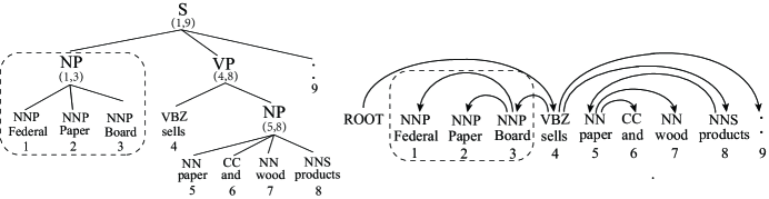
(a) Constituent and dependency.

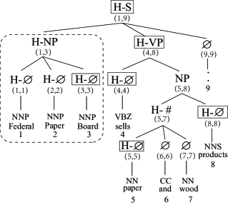
(b) Division span structure.

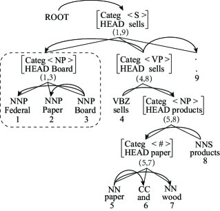
(c) Joint span structure.

Figure 3: Constituent, dependency and two different simplified HPSG structures of the same sentence which is indexed from 1 to 9 and assigned interval range for each node. Dotted box represents the same part. The special category $\#$ is assigned to divide the phrase with multiple heads. Division span structure adds token $H$ in front of the category to distinguish whether the phrase is on the left or right of the head. Thus the head is the last one of the category with $H$ which is marked with a box. Joint span structure contains constitute phrase and dependency arc. Categ in each node represents the category of each constituent and HEAD indicates the head word.

2.1 Tree Preprocessing

In standard HPSG relating to HFP, the HEAD value of any headed phrase is structure-shared with the HEAD value of the head daughter. In other words, the phrase in our simplified HPSG tree may be exactly the same as that in a constituent tree and the head word of the phrase corresponding to the parent of the head word of its children in dependency tree. For example, in the constituent tree of Figure 3(a), Federal Paper Board is a phrase $(1,3)$ assigned with category NP and in dependency tree, Board is parent of Federal and Paper, thus in our simplified HPSG tree, the head of phrase $(1,3)$ is Board.

For dependency parsing on PTB, the dependency structures are mainly obtained by converting constituent structure with three head rules: (1) Penn2Malt and the head rules of Yamada and Matsumoto (2003), noted as PTB-YM; (2) LTH Converter Johansson and Nugues (2007), noted as PTB-LTH; (3) Stanford parserDe Marneffe et al. (2006), noted as PTB-SD.

Following most of the recent work, we apply the PTB-SD representation converted by version 3.3.0 of the Stanford parser. However, this dependency representation results in around 1% of phrases containing two or three head words. As shown in Figure 3(a), the phrase (5,8) assigned with a category NP contains 2 head words of paper and products in dependency tree. In order to deal with the problem, we introduce a special category $\#$ to divide the phrase with multiple heads meeting only one head word for each phrase. After this conversion, only 50 heads are errors in Penn Treebank.

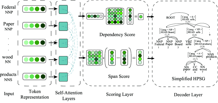
Figure 4: The framework of our joint span HPSG parsing model.

2.2 Span Representations of HPSG

Each node in the HPSG tree noted as AVM represents compound structure. Even in our simplified HPSG, each phrase (span) should be companied with its head. To facilitate the processing of existing parsers, we propose two ways to convert the simplified HPSG into a span-style tree structure.

Division Span A phrase is divided into two parts corresponding to left and right of its head. To distinguierrorsh the left and right parts, we add a special token $H$ in front of the category to indicate the left span, in which the head of the original phrase is always the last word. Since some leaves of the tree are without category, we explicitly use a special empty category $\O$ for their representation, and the token $H$ is also applied to the empty category.

As shown in Figure 3(b), the head of phrase (1,3) in the dotted box is Board, thus we add the special token $H$ in front of Federal, Paper and Board category. With this operation, head information has been encoded into span boundary of a standard constituent tree and we only need to parse such a constituent tree.

Joint Span We recursively define a structure called joint span to cover both constituent and head information. A joint span consists of all its children phrases and all dependency arcs between heads of all these children phrases.

For example, the HPSG node S_H(1, 9) in Figure 3(c) as a joint span is:

$$S_{H}(1,9)=\{S_{H}(1,3),S_{H}(4,8),S_{H}(9,9),$$

$$l(1,9),d(Board,sells),d(.,sells)\},$$

where $l$($i$, $j$) denotes category of span ($i$, $j$) and $d$($r$, $h$) indicates the dependency between the word $r$ and its parent $h$.

At last, following the recursive definition, the entire HPSG tree $T$ being a joint span can be represented as:

$$S_{H}(T)=\{S_{H}(1,9),d(sells,root)\}.$$

As all constituent and head information has been formally encoded into a span-like structure, we can use a constituent-like parser for such a joint span tree.

3 Our Model

3.1 Overview

Using an encoder-decoder backbone, our model apply self-attention encoder Vaswani et al. (2017) which is modified by position partition Kitaev and Klein (2018a). Since our two converted structures of simplified HPSG are based on the phrase, thus we can employ CKY-style Cocke (1969); Younger, Daniel H. (1975); Kasami, Tadao (1965) decoder for both to find the tree with the highest predicted scores. The difference is that for division span structure, we only need span scores while for joint span structure, we need both of span and dependency scores.

Given a sentence $s=\{w_{1},w_{2},\dots,w_{n}\}$, we attempt to predict a simplified HPSG tree. As shown in Figure 4, our parsing model includes four modules: token representation, self-attention encoder, scoring module and CKY-style decoder.

3.2 Token Representation

In our model, token representation $x_{i}$ is composed of character, word and part-of-speech (POS) embeddings. For character-level representation, we use CharLSTM Kitaev and Klein (2018a). For word-level representation, we concatenate randomly initialized and pre-trained word embeddings.

Finally, we concatenate character representation, word representation and POS embedding as our token representation:

$$x_{i}=[x_{char};x_{word};x_{POS}].$$

3.3 Self-Attention Encoder

The encoder in our model is adapted from Vaswani et al. (2017) and factor explicit content and position information in the self-attention process. The input matrices $X=[x_{1},x_{2},\dots,x_{n}]$ in which $x_{i}$ is concatenated with position embedding are transformed by a self-attention encoder. We factor the model between content and position information both in self-attention sub-layer and feed-forward network, whose setting details follow Kitaev and Klein (2018a).

3.4 Decoder for Division Span HPSG

After reconstructing of the HPSG tree as a constituent tree with head information as described in Section 2.2, we follow the constituent parsing as Kitaev and Klein (2018a); Gaddy et al. (2018) to predict constituent parse tree.

Firstly, we add a special empty category $\O$ to spans to binarize the n-ary nodes and apply a unary atomic category to deal with the nodes of the unary chain, corresponding to nested spans with the same endpoints.

Then, we train the span scorer. Span vector $s_{ij}$ is the concatenation of the vector differences $s_{ij}=[\overrightarrow{y_{j}}-\overrightarrow{y_{i-1}};\overleftarrow{y_{j+1}}-\overleftarrow{y_{i}}]$ which $\overrightarrow{y_{j}}$ is constructed by splitting in half the outputs from the self-attention encoder. We apply one-layer feedforward networks to generate span scores vector, taking span vector $s_{ij}$ as input:

$$S(i,j)=W_{2}g(LN(W_{1}s_{ij}+b_{1}))+b_{2},$$

where $LN$ denotes Layer Normalization, $g$ is the Rectified Linear Unit nonlinearity. The individual score of category $\ell$ is denoted by

$$S_{categ}(i,j,\ell)=[S(i,j)]_{\ell},$$

where $[]_{\ell}$ indicates the value of corresponding the element $\ell$ of the score vector. The score $s(T)$ of the constituent parse tree $T$ is to sum every scores of span ($i$, $j$) with category $\ell$:

$$s(T)=\sum_{(i,j,\ell)\in T}S_{categ}(i,j,\ell).$$

The goal of constituent parsing is to find the tree with the highest score: $\hat{T}=\arg\max_{T}s(T).$ We use CKY-style algorithm Stern et al. (2017a); Gaddy et al. (2018) to obtain the tree $\hat{T}$ in $O(n^{3})$ time complexity. This structured prediction problem is handled with satisfying the margin constraint:

$$s(T^{*})\geq s(T)+\Delta(T,T^{*}),$$

where $T^{*}$ denotes correct parse tree and $\Delta$ is the Hamming loss on category spans with a slight modification during the dynamic programming search. The objective function is the hinge loss,

$$J_{1}(\theta)=\max(0,\max_{T}[s(T)+\Delta(T,T^{*})]-s(T^{*})).$$

For dependency labels, following Dozat and Manning (2017), the classifier takes head and its children as features. We minimize the negative log probability of the correct dependency label $l_{i}$ for the child-parent pair $(x_{i},h_{i})$ implemented as cross-entropy loss:

$$J_{labels}(\theta)=-logP_{\theta}(l_{i}|x_{i},h_{i}).$$

Thus, the overall loss is sum of the objectives:

$$J_{Division}(\theta)=J_{1}(\theta)+J_{labels}(\theta).$$

Algorithm 1 Joint span parsing algorithm

0:  sentence leng $n$, span and dependency score $s(i,j,\ell)$, $d(r,h)$, $1\leq i\leq j\leq n,\forall r,h,\ell$

0:  maximum value $S_{H}(T)$ of tree $T$

  Initialization:

  $s_{c}[i][j][h]=s_{i}[i][j][h]=0,\forall i,j,h$

  for $len=1$ to $n$ do

     for $i=1$ to $n-len+1$ do

        $j=i+len-1$

        if $len=1$ then

           $\begin{aligned} s_{c}[i][j][i]=s_{i}[i][j][i]=\max_{\ell}s(i,j,\ell)\end{aligned}$

        else

           for $h=i$ to $j$ do

              $\begin{aligned} split_{l}=&\max_{i\leq r<h}\ \{\ \max_{r\leq k<h}\ \{\ s_{c}[i][k][r]+\\ &s_{i}[k+1][j][h]\ \}+d(r,h)\ \}\end{aligned}$

              $\begin{aligned} split_{r}=&\max_{h<r\leq j}\ \{\ \max_{h\leq k<r}\ \{\ s_{i}[i][k][h]+\\ &s_{c}[k+1][j][r]\ \}+d(r,h)\ \}\end{aligned}$

              $\begin{aligned} s_{c}[i][j][h]=&\max\ \{\ split_{l},split_{r}\ \}+\\ &\max_{\ell\neq\varnothing}s(i,j,\ell)\end{aligned}$

              $\begin{aligned} s_{i}[i][j][h]=&\max\ \{\ split_{l},split_{r}\ \}+\\ &\max_{\ell}s(i,j,\ell)\end{aligned}$

           end for

        end if

     end for

  end for

  $\begin{aligned} S_{H}(T)=\max_{1\leq h\leq n}\ \{\ s_{c}[1][n][h]+d(h,root)\ \}\end{aligned}$

3.5 Decoder for Joint Span HPSG

As our joint span is defined in a recursive way, to score the root joint span has been equally scoring all spans and dependencies in the HPSG tree.

For span scores, we continuously apply the approach and hinge loss $J_{1}(\theta)$ in the previous section. For dependency scores, we predict a distribution over the possible head for each word and use the biaffine attention mechanism Dozat and Manning (2017) to calculate the score as follow:

$$\alpha_{ij}=h_{i}^{T}Wg_{j}+U^{T}h_{i}+V^{T}g_{j}+b,$$

where $\alpha_{ij}$ indicates the child-parent score, $W$ denotes the weight matrix of the bi-linear term, $U$ and $V$ are the weight vectors of the linear term and $b$ is the bias item, $h_{i}$ and $g_{i}$ are calculated by a distinct one-layer perceptron network.

We minimize the negative log-likelihood of the golden dependency tree $Y$, which is implemented as a cross-entropy loss:

$$J_{2}(\theta)=-\left(logP_{\theta}(h_{i}|x_{i})+logP_{\theta}(l_{i}|x_{i},h_{i})\right),$$

where $P_{\theta}(h_{i}|x_{i})$ is the probability of correct parent node $h_{i}$ for $x_{i}$, and $P_{\theta}(l_{i}|x_{i},h_{i})$ is the probability of the correct dependency label $l_{i}$ for the child-parent pair $(x_{i},h_{i})$. To predict span and dependency scores simultaneously, we jointly train our parser for minimizing the overall loss:

$$J_{Joint}(\theta)=J_{1}(\theta)+J_{2}(\theta).$$

During testing, we propose a CKY-style algorithm as shown in Algorithm 1 to explicitly find the globally highest span and dependency score $S_{H}(T)$ of our simplified HPSG tree $T$. In order to binarize the constituent parse tree with head, we introduce the complete span $s_{c}$ and the incomplete span $s_{i}$ which is similar to Eisner algorithm Eisner (1996). After finding the best score $S_{H}(T)$, we backtrack the chart with split point $k$ and sub-root $r$ to construct the simplified HPSG tree $T$.

Comparing with constituent parsing CKY-style algorithm Stern et al. (2017a), the dependency score $d(r,h)$ in our algorithm affects the selection of best split point $k$. Since we need to find the best value of sub-head $r$ and split point $k$, the complexity of the algorithm is $O(n^{5})$ time and $O(n^{3})$ space. To control the effect of combining span and dependency scores, we apply a weight $\lambda$:

$$s(i,j,\ell)=\lambda S_{categ}(i,j,\ell),d(i,j)=(1.0-\lambda)\alpha_{ij},$$

where $\lambda$ in the range of 0 to 1. In addition, we can merely generate constituent or dependency parsing tree by setting $\lambda$ to 1 or 0, respectively.

4 Experiments

In order to evaluate the proposed model, we convert our simplified HPSG tree to constituent and dependency parse trees and evaluate on two benchmark treebanks, English Penn Treebank (PTB) and Chinese Penn Treebank (CTB5.1) following standard data splitting Zhang and Clark (2008); Liu and Zhang (2017b). The placeholders with the -NONE- tag are stripped from the CTB. POS tags are predicted using the Stanford tagger Toutanova et al. (2003) and we use the same pretagged dataset as Cross and Huang (2016) for PTB. For CTB, we use golden POS tags for dependency parsing and predicted POS tags for constituent parsing.

For constituent parsing, we use the standard evalb tool to evaluate the F1 score. For dependency parsing, following Dozat and Manning (2017); Kuncoro et al. (2016); Ma et al. (2018), we report the results without punctuations for both treebanks.

4.1 Setup

Hyperparameters In our experiments, we use 100D GloVe Pennington et al. (2014) and structured-skipgram Ling et al. (2015) pre-train embeddings for English and Chinese respectively. The character representations are randomly initialized, and the dimension is 64. For self-attention encoder, we use the same hyperparameters settings as Kitaev and Klein (2018a).

For span scores, we apply a hidden size of 250-dimensional feed-forward networks. For dependency biaffine scores, we employ two 1024-dimensional MLP layers with the ReLU as the activation function and a 1024-dimensional parameter matrix for biaffine attention. In addition, we augment our parser with ELMo Peters et al. (2018), a larger version of BERT Devlin et al. (2018) (24 layers, 16 attention heads per layer, and 1024-dimensional hidden vectors) and XLNet Yang et al. (2019) to compare with other pre-trained or ensemble models. We set 4 layers of self-attention for ELMo and 2 layers of self-attention for BERT or XLNet as Kitaev and Klein (2018a, b).

Training Details we use 0.33 dropout for biaffine attention and MLP layers. All models are trained for up to 150 epochs with batch size 150 on a single NVIDIA GeForce GTX 1080Ti GPU with Intel i7-7800X CPU. We use the same training settings as Kitaev and Klein (2018a) and Kitaev and Klein (2018b).

Self-attention Layers	F1	UAS	LAS
Division Span Model
8 self-attention layers	93.42	94.05	92.68
12 self-attention layers	93.57	94.40	93.05
16 self-attention layers	93.36	94.08	92.66
Joint Span Model
8 self-attention layers	93.64	95.75	94.36
12 self-attention layers	93.78	95.92	94.49
16 self-attention layers	93.54	95.54	94.21

Table 1: Different self-attention layers on English dev set.

4.2 Self-attention Layers

This subsection examines the impact of different numbers of self-attention layers varying from 8 to 16. The comparison in Table 1 indicates that the best performing setting comes from 12 self-attention layers, and more than 12 layers shows almost no promotion even reduces the accuracy. Thus the rest experiments are done with 12 layers of the self-attention encoder.

4.3 Moderating constituent and Dependency

The weight parameter $\lambda$ plays an important role to balance the scoring of span and dependency. When $\lambda$ set to 0, indicates only using dependency score to generate dependency tree as the general first-order dependency parsing Eisner (1996), while $\lambda$ set to 1, shows the constituent parsing only. $\lambda$ set to between 0 to 1 indicates our general simplified HPSG parsing, providing both constituent and dependency structure prediction.

The comparison in Figure 5 shows that our HPSG decoder is better than either separate constituent or dependency decoder, which shows the bonus of joint predicting constituent and dependency. Moreover, $\lambda$ set to 0.5 achieves the best performance in terms of both F1 score and UAS.

Model	F1	UAS	LAS
separate constituent	93.47	-	-
converted dependency		95.06	93.81
joint span $\lambda$ = 1.0	93.67	-	-
joint span $\lambda$ = 0.0	-	95.82	94.43
joint span $\lambda$ = 0.5	93.78	95.92	94.49
converted dependency		95.69	94.45

Table 2: English dev set performance of joint span HPSG parsing. The converted means the corresponding dependency parsing results are from the corresponding constituent parse tree using head rules.

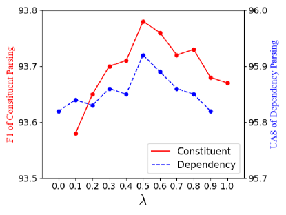
Figure 5: Balancing constituent and dependency of joint span HPSG parsing on English dev set.

4.4 Joint Span HPSG Parsing

We compare our join span HPSG parser with a separate learning constituent parsing model which takes the same token representation and self-attention encoder on PTB dev set. The constituent parsing results are also converted into dependency ones by PTB-SD for comparison.

When $\lambda$ is set to 0 and 1, our joint span HPSG parser works as the dependency-only parser and constituent-only parser respectively. Table 3 shows that even in such a work mode, our HPSG parser still outperforms the separate constituent parser in terms of either constituent and dependency parsing performance.

As $\lambda$ is set to 0.5, our HPSG parser will give constituent and dependency structures at the same time, which are shown better than the work alone mode of either constituent or dependency parsing. Besides, the comparison also shows that the directly predicted dependencies from our model are slightly better than those converted from the predicted constituent parse trees.

Model	sents/sec
Petrov and Klein (2007)	6.2
Zhu et al. (2013)	89.5
Liu and Zhang (2017b)	79.2
Stern et al. (2017a)	75.5
Shen et al. (2018)	111.1
Shen et al. (2018)(w/o tree inference)	351
Our (Division)	226.3
Our (Joint)	158.7

Table 3: Parsing speed on the PTB dataset.

Model	English		Chinese
	UAS	LAS	UAS	LAS
Chen and Manning (2014)	91.8	89.6	83.9	82.4
Andor et al. (2016)	94.61	92.79	_	_
Zhang et al. (2016)	93.42	91.29	87.65	86.17
Cheng et al. (2016)	94.10	91.49	88.1	85.7
Kuncoro et al. (2016)	94.26	92.06	88.87	87.30
Ma and Hovy (2017)	94.88	92.98	89.05	87.74
Dozat and Manning (2017)	95.74	94.08	89.30	88.23
Li et al. (2018a)	94.11	92.08	88.78	86.23
Ma et al. (2018)	95.87	94.19	90.59	89.29
Pointer Networks	96.04	94.43	-	-
Our (Division)	94.32	93.09	89.14	87.31
Our (Joint)	96.09	94.68	91.21	89.15
Our (Division*)	-	-	91.69	90.54
Our (Joint*)	-	-	93.24	91.95
Pre-training/Ensemble
Choe and Charniak (2016)	95.9	94.1	_	_
Kuncoro et al. (2017)	95.8	94.6	_	_
Wang et al. (2018b)(ELMo)	96.35	95.25	_	_
Our (Division) + ELMo	95.77	94.21	-	-
Our (Joint) + ELMo	96.76	94.93	-	-
Our (Division) + BERT	96.22	94.56	-	-
Our (Joint) + BERT	97.00	95.43	-	-
Our (Joint) + XLNet	97.20	95.72	-	-

Table 4: Dependency parsing on PTB and CTB test set. * represents CTB constituent data splitting. Pointer Networks represents the results of Fernández-González and Gómez-Rodríguez (2019).

4.5 Parsing Speed

We compare the parsing speed of our parser with other neural parsers in Table 3. Although the time complexity of our Joint span model is $O(n^{5})$, there is not much slower than Division span model with $O(n^{3})$ time complexity. The comparison suggests that training and inference times are dominated by neural network computations and our decoder consumes a small fraction of total running time.

4.6 Main Results

Tables 4, 5 and 6 compare our model to existing state-of-the-art on test sets. Division and Joint indicate the results of division and joint span parsing respectively. On PTB, our best model achieves new state-of-the-art on both constituent and dependency parsing. On CTB, our best model achieves 89.40 F1 score of constituent parsing and 91.21% UAS and 89.15% LAS of dependency parsing. Since constituent and dependency parsing have different data splitting on CTB Zhang and Clark (2008); Liu and Zhang (2017b), we report our parsing performance on both data splitting.

The comparison shows that our HPSG parsing model is more effective than learning constituent or dependency parsing separately. We also find that dependency parsing is shown much more beneficial from Joint than Division way which empirically suggests dependency score in our joint loss is helpful.

We augment our parser with ELMo, a larger version of BERT and XLNet as the sole token representation to compare with other models. Our Joint model in XLNet setting even defeats other ensemble models of both constituent and dependency parsing achieving 96.33 F1 score, 97.20% UAS and 95.72% LAS.

For fair comparison with other pre-train model on constituent parsing, we also augment our parser with Chinese larger version of RoBERTa as the sole token representation. Our Joint model in RoBERTa setting achieves the state of art performance of 92.55 F1 score on constituent parsing.

Model	LR	LP	F1
Zhu et al. (2013)	90.7	90.2	90.4
Dyer et al. (2016)	_	_	89.8
Cross and Huang (2016)	90.5	92.1	91.3
Stern et al. (2017a)	93.2	90.3	91.8
Gaddy et al. (2018)	91.76	92.41	92.08
Stern et al. (2017b)	92.57	92.56	92.56
Kitaev and Klein (2018a)	93.20	93.90	93.55
Our (Division)	93.41	93.87	93.64
Our (Joint)	93.64	93.92	93.78
Pre-training/Ensemble
Dyer et al. (2016)	_	_	93.3
Choe and Charniak (2016)	_	_	93.8
Liu and Zhang (2017a)	_	_	94.2
Fried et al. (2017)	_	_	94.66
Kitaev and Klein (2018a)
+ ELMo	94.85	95.40	95.13
Kitaev and Klein (2018b)
+ BERT	95.46	95.73	95.59
Kitaev and Klein (2018b)	95.51	96.03	95.77
Our (Division) + ELMo	94.54	95.68	95.10
Our (Joint) + ELMo	95.04	95.39	95.22
Our (Division) + BERT	95.51	95.93	95.72
Our (Joint) + BERT	95.70	95.98	95.84
Our (Joint) + XLNet	96.21	96.46	96.33

Table 5: Constituent parsing on PTB test set.

Model	LR	LP	F1
Wang et al. (2015)	_	_	83.2
Dyer et al. (2016)	_	_	84.6
Liu and Zhang (2017b)	85.9	85.2	85.5
Liu and Zhang (2017a)	_	_	86.1
Shen et al. (2018)	86.6	86.4	86.5
Fried and Klein (2018)	_	_	87.0
Teng and Zhang (2018)	87.1	87.5	87.3
Kitaev and Klein (2018b)	91.55	91.96	91.75
Our (Division)	88.75	89.79	89.27
Our (Joint)	89.09	89.70	89.40
+ RoBERTa	92.50	92.61	92.55
Our (Division*)	87.41	88.07	87.74
Our (Joint*)	87.87	87.96	87.92
+ RoBERTa	90.14	89.89	90.02

Table 6: Constituent parsing on CTB test set. * represents CTB dependency data splitting.

5 Related Work

In the earlier time, linguists and NLP researchers discussed how to encode lexical dependencies in phrase structures, like lexicalized tree adjoining grammar (LTAG) Schabes et al. (1988) and head-driven phrase structure grammar (HPSG) Pollard and Sag (1994) which is a constraint-based highly lexicalized non-derivational generative grammar framework.

In the past decade, there was a lot of large-scale HPSG-based NLP parsing systems which had been built. Such as the Enju English and Chinese parser Miyao et al. (2004); Yu et al. (2010), the Alpino parser for Dutch Van Noord et al. (2006), and the LKB & PET Copestake (2002); Callmeier (2000) for English, German, and Japanese..

Meanwhile, since HPSG represents the grammar framework in a precisely constrained way, it is difficult to broadly cover unseen real-world texts for parsing. Consequently, according to Zhang and Krieger (2011), many of these large-scale grammar implementations are forced to choose to either compromise the linguistic preciseness or to accept the low coverage in parsing. Previous works of HPSG approximation focus on two major approaches: grammar based approach Kiefer and Krieger (2004), and the corpus-driven approach Krieger (2007) and Zhang and Krieger (2011) which proposes PCFG approximation as a way to alleviate some of these issues in HPSG processing.

Recently, with the impressive success of deep neural networks in a wide range of NLP tasks Li et al. (2018b); Zhang et al. (2018a); Li et al. (2018c); Zhang et al. (2018c, b); Zhang and Zhao (2018); Cai et al. (2018); He et al. (2018); Xiao et al. (2019); Chen et al. (2018); Wang et al. (2018, 2018a, 2017b, 2017a), constituent and dependency parsing have been well developed with neural network. These models attain state-of-the-art results for dependency parsing Chen and Manning (2014); Dozat and Manning (2017); Ma et al. (2018) and constituent parsing Dyer et al. (2016); Cross and Huang (2016); Kitaev and Klein (2018a).

Since constituent and dependency share a lot of grammar and machine learning characteristics, it is a natural idea to study the relationship between constituent and dependency structures, and the joint learning of constituent and dependency parsing Collins (1997); Charniak (2000); Charniak and Johnson (2005); Farkas et al. (2011); Green and Žabokrtský (2012); Ren et al. (2013); Yoshikawa et al. (2017).

To further exploit both strengths of the two representation forms, in this work, for the first time, we propose a graph-based parsing model that formulates constituent and dependency structures as simplified HPSG.

6 Conclusions

This paper presents a simplified HPSG with two different decode methods which are evaluated on both constituent and dependency parsing. Despite the usefulness of HPSG in practice and its theoretical linguistic background, our model achieves new state-of-the-art results on both Chinese and English benchmark treebanks of both parsing tasks. Thus, this work is more than proposing a high-performance parsing model by exploring the relation between constituent and dependency structures. Our experiments show that joint learning of constituent and dependency is indeed superior to separate learning mode, and combining constituent and dependency score in joint training to parse a simplified HPSG can obtain further performance improvement.

References

- Andor et al. (2016) Daniel Andor, Chris Alberti, David Weiss, Aliaksei Severyn, Alessandro Presta, Kuzman Ganchev, Slav Petrov, and Michael Collins. 2016. Globally Normalized Transition-Based Neural Networks. In Proceedings of the 54th Annual Meeting of the Association for Computational Linguistics (ACL), pages 2442–2452.
- Bresnan et al. (2015) Joan Bresnan, Ash Asudeh, Ida Toivonen, and Stephen Wechsler. 2015. Lexical-functional syntax, volume 16. John Wiley & Sons.
- Cai et al. (2018) Jiaxun Cai, Shexia He, Zuchao Li, and Hai Zhao. 2018. A Full End-to-End Semantic Role Labeler, Syntactic-agnostic Over Syntactic-aware? In Proceedings of the 27th International Conference on Computational Linguistics (COLING), pages 2753–2765.
- Callmeier (2000) Ulrich Callmeier. 2000. PET - A platform for experimentation with efficient HPSG processing techniques. Natural Language Engineering, 6(1):99–107.
- Charniak (2000) Eugene Charniak. 2000. A Maximum-Entropy-Inspired Parser. In 1st Meeting of the North American Chapter of the Association for Computational Linguistics (NAACL).
- Charniak and Johnson (2005) Eugene Charniak and Mark Johnson. 2005. Coarse-to-Fine n-Best Parsing and MaxEnt Discriminative Reranking. In Proceedings of the 43rd Annual Meeting of the Association for Computational Linguistics (ACL), pages 173–180.
- Chen and Manning (2014) Danqi Chen and Christopher Manning. 2014. A Fast and Accurate Dependency Parser using Neural Networks. In Proceedings of the 2014 Conference on Empirical Methods in Natural Language Processing (EMNLP), pages 740–750.
- Chen et al. (2018) Kehai Chen, Rui Wang, Masao Utiyama, Eiichiro Sumita, and Tiejun Zhao. 2018. Syntax-Directed Attention for Neural Machine Translation. In Proceedings of the AAAI Conference on Artificial Intelligence, pages 4792–4799.
- Cheng et al. (2016) Hao Cheng, Hao Fang, Xiaodong He, Jianfeng Gao, and Li Deng. 2016. Bi-directional Attention with Agreement for Dependency Parsing. In Proceedings of the 2016 Conference on Empirical Methods in Natural Language Processing (EMNLP), pages 2204–2214.
- Choe and Charniak (2016) Do Kook Choe and Eugene Charniak. 2016. Parsing as Language Modeling. In Proceedings of the 2016 Conference on Empirical Methods in Natural Language Processing (EMNLP), pages 2331–2336.
- Chomsky (1981) N. Chomsky. 1981. Lectures on Government and Binding. Mouton de Gruyter.
- Cocke (1969) John Cocke. 1969. Programming Languages and Their Compilers: Preliminary Notes. New York University.
- Collins (1997) Michael Collins. 1997. Three Generative, Lexicalised Models for Statistical Parsing. In 35th Annual Meeting of the Association for Computational Linguistics (ACL).
- Copestake (2002) Ann Copestake. 2002. Implementing Typed Feature Structure Grammars, volume 110. CSLI publications Stanford.
- Cross and Huang (2016) James Cross and Liang Huang. 2016. Span-Based Constituency Parsing with a Structure-Label System and Provably Optimal Dynamic Oracles . In Proceedings of the 2016 Conference on Empirical Methods in Natural Language Processing (EMNLP), pages 1–11.
- De Marneffe et al. (2006) Marie-Catherine De Marneffe, Bill MacCartney, Christopher D Manning, et al. 2006. Generating Typed Dependency Parses from Phrase Structure Parses. In Lrec, volume 6, pages 449–454.
- Devlin et al. (2018) Jacob Devlin, Ming-Wei Chang, Kenton Lee, and Kristina Toutanova. 2018. BERT: Pre-training of Deep Bidirectional Transformers for Language Understanding. abs/1810.04805.
- Dozat and Manning (2017) Timothy Dozat and Christopher D Manning. 2017. Deep Biaffine Attention for Neural Dependency Parsing. arXiv preprint arXiv:1611.01734.
- Dyer et al. (2016) Chris Dyer, Adhiguna Kuncoro, Miguel Ballesteros, and Noah A. Smith. 2016. Recurrent Neural Network Grammars. In Proceedings of the 2016 Conference of the North American Chapter of the Association for Computational Linguistics: Human Language Technologies (NAACL), pages 199–209.
- Eisner (1996) Jason Eisner. 1996. Efficient Normal-Form Parsing for Combinatory Categorial Grammar. In 34th Annual Meeting of the Association for Computational Linguistics (ACL).
- Farkas et al. (2011) Richàrd Farkas, Bernd Bohnet, and Helmut Schmid. 2011. Features for Phrase-Structure Reranking from Dependency Parses. In Proceedings of the 12th International Conference on Parsing Technologies, pages 209–214.
- Fernández-González and Gómez-Rodríguez (2019) Daniel Fernández-González and Carlos Gómez-Rodríguez. 2019. Left-to-Right Dependency Parsing with Pointer Networks. abs/1903.08445.
- Fried and Klein (2018) Daniel Fried and Dan Klein. 2018. Policy Gradient as a Proxy for Dynamic Oracles in Constituency Parsing. In Proceedings of the 56th Annual Meeting of the Association for Computational Linguistics (ACL), pages 469–476.
- Fried et al. (2017) Daniel Fried, Mitchell Stern, and Dan Klein. 2017. Improving Neural Parsing by Disentangling Model Combination and Reranking Effects . In Proceedings of the 55th Annual Meeting of the Association for Computational Linguistics (ACL), pages 161–166.
- Gaddy et al. (2018) David Gaddy, Mitchell Stern, and Dan Klein. 2018. What’s Going On in Neural Constituency Parsers? An Analysis. In Proceedings of the 2018 Conference of the North American Chapter of the Association for Computational Linguistics: Human Language Technologies (NAACL: HLT), pages 999–1010.
- Green and Žabokrtský (2012) Nathan Green and Zdeněk Žabokrtský. 2012. Hybrid Combination of Constituency and Dependency Trees into an Ensemble Dependency Parser. In Proceedings of the Workshop on Innovative Hybrid Approaches to the Processing of Textual Data, pages 19–26.
- He et al. (2018) Shexia He, Zuchao Li, Hai Zhao, and Hongxiao Bai. 2018. Syntax for Semantic Role Labeling, To Be, Or Not To Be. In Proceedings of the 56th Annual Meeting of the Association for Computational Linguistics (ACL), pages 2061–2071.
- Johansson and Nugues (2007) Richard Johansson and Pierre Nugues. 2007. Extended Constituent-to-Dependency Conversion for English. In Proceedings of the 16th Nordic Conference of Computational Linguistics (NODALIDA 2007), pages 105–112.
- Kasami, Tadao (1965) Kasami, Tadao. 1965. An Efficient Recognition and Syntax-Analysis Algorithm for Context-Free Languages. Technical Report Air Force Cambridge Research Lab.
- Kiefer and Krieger (2004) Bernd Kiefer and Hans-Ulrich Krieger. 2004. A Context-Free Superset Approximation of Unification-Based Grammars. In New developments in parsing technology, pages 229–250.
- Kitaev and Klein (2018a) Nikita Kitaev and Dan Klein. 2018a. Constituency Parsing with a Self-Attentive Encoder. In Proceedings of the 56th Annual Meeting of the Association for Computational Linguistics (ACL), pages 2676–2686.
- Kitaev and Klein (2018b) Nikita Kitaev and Dan Klein. 2018b. Multilingual Constituency Parsing with Self-Attention and Pre-Training. arXiv preprint arXiv:1812.11760.
- Krieger (2007) Hans-Ulrich Krieger. 2007. From UBGs to CFGs A practical corpus-driven approach. Natural Language Engineering, 13(4):317–351.
- Kuncoro et al. (2017) Adhiguna Kuncoro, Miguel Ballesteros, Lingpeng Kong, Chris Dyer, Graham Neubig, and Noah A. Smith. 2017. What Do Recurrent Neural Network Grammars Learn About Syntax? In Proceedings of the 15th Conference of the European Chapter of the Association for Computational Linguistics: Volume 1, Long Papers (EACL), pages 1249–1258.
- Kuncoro et al. (2016) Adhiguna Kuncoro, Miguel Ballesteros, Lingpeng Kong, Chris Dyer, and Noah A. Smith. 2016. Distilling an Ensemble of Greedy Dependency Parsers into One MST Parser. In Proceedings of the 2016 Conference on Empirical Methods in Natural Language Processing (EMNLP), pages 1744–1753.
- Li et al. (2018a) Zuchao Li, Jiaxun Cai, Shexia He, and Hai Zhao. 2018a. Seq2seq Dependency Parsing. In Proceedings of the 27th International Conference on Computational Linguistics (COLING), pages 3203–3214.
- Li et al. (2018b) Zuchao Li, Shexia He, Jiaxun Cai, Zhuosheng Zhang, Hai Zhao, Gongshen Liu, Linlin Li, and Luo Si. 2018b. A Unified Syntax-aware Framework for Semantic Role Labeling. In Proceedings of the 2018 Conference on Empirical Methods in Natural Language Processing (EMNLP), pages 2401–2411.
- Li et al. (2018c) Zuchao Li, Shexia He, Zhuosheng Zhang, and Hai Zhao. 2018c. Joint Learning of POS and Dependencies for Multilingual Universal Dependency Parsing. In Proceedings of the CoNLL 2018 Shared Task: Multilingual Parsing from Raw Text to Universal Dependencies (CONLL), pages 65–73.
- Ling et al. (2015) Wang Ling, Chris Dyer, Alan W Black, and Isabel Trancoso. 2015. Two/Too Simple Adaptations of Word2Vec for Syntax Problems. In Proceedings of the 2015 Conference of the North American Chapter of the Association for Computational Linguistics: Human Language Technologies (NAACL: HLT), pages 1299–1304.
- Liu and Zhang (2017a) Jiangming Liu and Yue Zhang. 2017a. In-Order Transition-based Constituent Parsing. Transactions of the Association for Computational Linguistics (TACL), 5:413–424.
- Liu and Zhang (2017b) Jiangming Liu and Yue Zhang. 2017b. Shift-Reduce Constituent Parsing with Neural Lookahead Features. Transactions of the Association for Computational Linguistics (TACL), 5:45–58.
- Ma and Hovy (2017) Xuezhe Ma and Eduard Hovy. 2017. Neural Probabilistic Model for Non-projective MST Parsing. In Proceedings of the Eighth International Joint Conference on Natural Language Processing (IJCNLP), pages 59–69.
- Ma et al. (2018) Xuezhe Ma, Zecong Hu, Jingzhou Liu, Nanyun Peng, Graham Neubig, and Eduard Hovy. 2018. Stack-Pointer Networks for Dependency Parsing. In Proceedings of the 56th Annual Meeting of the Association for Computational Linguistics (ACL), pages 1403–1414.
- Ma et al. (2010) Xuezhe Ma, Xiaotian Zhang, Hai Zhao, and Bao-Liang Lu. 2010. Dependency Parser for Chinese Constituent Parsing. In CIPS-SIGHAN Joint Conference on Chinese Language Processing (CLP).
- Marcus et al. (1993) Mitchell P. Marcus, Beatrice Santorini, and Mary Ann Marcinkiewicz. 1993. Building a Large Annotated Corpus of English: The Penn Treebank. Computational Linguistics, 19(2).
- Miyao et al. (2004) Yusuke Miyao, Takashi Ninomiya, and Jun’ichi Tsujii. 2004. Corpus-Oriented Grammar Development for Acquiring a Head-Driven Phrase Structure Grammar from the Penn Treebank. In International Conference on Natural Language Processing (IJCNLP), pages 684–693.
- Pennington et al. (2014) Jeffrey Pennington, Richard Socher, and Christopher Manning. 2014. Glove: Global Vectors for Word Representation. In Proceedings of the 2014 Conference on Empirical Methods in Natural Language Processing (EMNLP), pages 1532–1543.
- Peters et al. (2018) Matthew Peters, Mark Neumann, Mohit Iyyer, Matt Gardner, Christopher Clark, Kenton Lee, and Luke Zettlemoyer. 2018. Deep Contextualized Word Representations. In Proceedings of the 2018 Conference of the North American Chapter of the Association for Computational Linguistics: Human Language Technologies (NAACL: HLT), pages 2227–2237.
- Petrov and Klein (2007) Slav Petrov and Dan Klein. 2007. Improved Inference for Unlexicalized Parsing. In Human Language Technologies 2007: The Conference of the North American Chapter of the Association for Computational Linguistics; Proceedings of the Main Conference (NAACL), pages 404–411.
- Pollard and Sag (1994) Carl Pollard and Ivan A Sag. 1994. Head-Driven Phrase Structure Grammar. University of Chicago Press.
- Ren et al. (2013) Xiaona Ren, Xiao Chen, and Chunyu Kit. 2013. Combine Constituent and Dependency Parsing via Reranking. In Proceedings of the Twenty-Third International Joint Conference on Artificial Intelligence (IJCAI), pages 2155–2161.
- Schabes et al. (1988) Yves Schabes, Anne Abeille, and Aravind K. Joshi. 1988. Parsing strategies with ’lexicalized’ grammars: Application to tree adjoining grammars. In Coling Budapest 1988 Volume 2: International Conference on Computational Linguistics (COLING).
- Shen et al. (2018) Yikang Shen, Zhouhan Lin, Athul Paul Jacob, Alessandro Sordoni, Aaron Courville, and Yoshua Bengio. 2018. Straight to the Tree: Constituency Parsing with Neural Syntactic Distance. In Proceedings of the 56th Annual Meeting of the Association for Computational Linguistics (ACL), pages 1171–1180.
- Stern et al. (2017a) Mitchell Stern, Jacob Andreas, and Dan Klein. 2017a. A Minimal Span-Based Neural Constituency Parser. In Proceedings of the 55th Annual Meeting of the Association for Computational Linguistics (ACL), pages 818–827.
- Stern et al. (2017b) Mitchell Stern, Daniel Fried, and Dan Klein. 2017b. Effective Inference for Generative Neural Parsing. In Proceedings of the 2017 Conference on Empirical Methods in Natural Language Processing (EMNLP), pages 1695–1700.
- Teng and Zhang (2018) Zhiyang Teng and Yue Zhang. 2018. Two Local Models for Neural Constituent Parsing. In Proceedings of the 27th International Conference on Computational Linguistics (COLING), pages 119–132.
- Toutanova et al. (2003) Kristina Toutanova, Dan Klein, Christopher D. Manning, and Yoram Singer. 2003. Feature-rich Part-of-speech Tagging with a Cyclic Dependency Network. In Proceedings of the 2003 Conference of the North American Chapter of the Association for Computational Linguistics on Human Language Technology (NAACL), pages 173–180.
- Van Noord et al. (2006) Gertjan Van Noord et al. 2006. At Last Parsing is Now Operational. In TALN06. Verbum Ex Machina. Actes de la 13e conference sur le traitement automatique des langues naturelles, pages 20–42.
- Vaswani et al. (2017) Ashish Vaswani, Noam Shazeer, Niki Parmar, Jakob Uszkoreit, Llion Jones, Aidan N Gomez, Ł ukasz Kaiser, and Illia Polosukhin. 2017. Attention is All you Need. In Advances in Neural Information Processing Systems (NIPS), pages 5998–6008.
- Wang et al. (2017a) Rui Wang, Andrew Finch, Masao Utiyama, and Eiichiro Sumita. 2017a. Sentence Embedding for Neural Machine Translation Domain Adaptation. In Proceedings of the 55th Annual Meeting of the Association for Computational Linguistics (ACL), pages 560–566.
- Wang et al. (2018) Rui Wang, Masao Utiyama, Andrew Finch, Lemao Liu, Kehai Chen, and Eiichiro Sumita. 2018. Sentence Selection and Weighting for Neural Machine Translation Domain Adaptation. IEEE/ACM Transactions on Audio, Speech, and Language Processing, 26(10):1727–1741.
- Wang et al. (2017b) Rui Wang, Masao Utiyama, Lemao Liu, Kehai Chen, and Eiichiro Sumita. 2017b. Instance Weighting for Neural Machine Translation Domain Adaptation. In Proceedings of the 2017 Conference on Empirical Methods in Natural Language Processing (EMNLP), pages 1482–1488.
- Wang et al. (2018a) Rui Wang, Masao Utiyama, and Eiichiro Sumita. 2018a. Dynamic Sentence Sampling for Efficient Training of Neural Machine Translation. In Proceedings of the 56th Annual Meeting of the Association for Computational Linguistics (ACL), pages 298–304.
- Wang et al. (2018b) Wenhui Wang, Baobao Chang, and Mairgup Mansur. 2018b. Improved Dependency Parsing using Implicit Word Connections Learned from Unlabeled Data. In Proceedings of the 2018 Conference on Empirical Methods in Natural Language Processing (EMNLP), pages 2857–2863.
- Wang et al. (2015) Zhiguo Wang, Haitao Mi, and Nianwen Xue. 2015. Feature Optimization for Constituent Parsing via Neural Networks. In Proceedings of the 53rd Annual Meeting of the Association for Computational Linguistics and the 7th International Joint Conference on Natural Language Processing (ACL-IJCNLP), pages 1138–1147.
- Xiao et al. (2019) Fengshun Xiao, Jiangtong Li, Hai Zhao, Rui Wang, and Kehai Chen. 2019. Lattice-Based Transformer Encoder for Neural Machine Translation. In Proceedings of the 57th Annual Meeting of the Association for Computational Linguistics (ACL).
- Yang et al. (2019) Zhilin Yang, Zihang Dai, Yiming Yang, Jaime G. Carbonell, Ruslan Salakhutdinov, and Quoc V. Le. 2019. XLNet: Generalized Autoregressive Pretraining for Language Understanding. abs/1906.08237.
- Yoshikawa et al. (2017) Masashi Yoshikawa, Hiroshi Noji, and Yuji Matsumoto. 2017. A* CCG Parsing with a Supertag and Dependency Factored Model. In Proceedings of the 55th Annual Meeting of the Association for Computational Linguistics (ACL), pages 277–287.
- Younger, Daniel H. (1975) Younger, Daniel H. 1975. Recognition and Parsing of Context-Free Languages in Time n3. Information & Control, 10(2):189–208.
- Yu et al. (2010) Kun Yu, Yusuke Miyao, Xiangli Wang, Takuya Matsuzaki, and Junichi Tsujii. 2010. Semi-automatically developing Chinese HPSG grammar from the Penn Chinese treebank for deep parsing. In Coling 2010: Posters, pages 1417–1425.
- Zhang and Krieger (2011) Yi Zhang and Hans-Ulrich Krieger. 2011. Large-Scale Corpus-Driven PCFG Approximation of an HPSG. In Proceedings of the 12th International Conference on Parsing Technologies, pages 198–208.
- Zhang and Clark (2008) Yue Zhang and Stephen Clark. 2008. A Tale of Two Parsers: Investigating and Combining Graph-based and Transition-based Dependency Parsing. In Proceedings of the 2008 Conference on Empirical Methods in Natural Language Processing (EMNLP), pages 562–571.
- Zhang et al. (2018a) Zhisong Zhang, Rui Wang, Masao Utiyama, Eiichiro Sumita, and Hai Zhao. 2018a. Exploring Recombination for Efficient Decoding of Neural Machine Translation. In Proceedings of the 2018 Conference on Empirical Methods in Natural Language Processing (EMNLP), pages 4785–4790.
- Zhang et al. (2016) Zhisong Zhang, Hai Zhao, and Lianhui Qin. 2016. Probabilistic Graph-based Dependency Parsing with Convolutional Neural Network. In Proceedings of the 54th Annual Meeting of the Association for Computational Linguistics (ACL), pages 1382–1392.
- Zhang et al. (2018b) Zhuosheng Zhang, Yafang Huang, and Hai Zhao. 2018b. Subword-augmented Embedding for Cloze Reading Comprehension. In Proceedings of the 27th International Conference on Computational Linguistics (COLING), pages 1802–1814.
- Zhang et al. (2018c) Zhuosheng Zhang, Jiangtong Li, Pengfei Zhu, Hai Zhao, and Gongshen Liu. 2018c. Modeling Multi-turn Conversation with Deep Utterance Aggregation. In Proceedings of the 27th International Conference on Computational Linguistics (COLING), pages 3740–3752.
- Zhang and Zhao (2018) Zhuosheng Zhang and Hai Zhao. 2018. One-shot Learning for Question-Answering in Gaokao History Challenge. In Proceedings of the 27th International Conference on Computational Linguistics (COLING), pages 449–461.
- Zhu et al. (2013) Muhua Zhu, Yue Zhang, Wenliang Chen, Min Zhang, and Jingbo Zhu. 2013. Fast and Accurate Shift-Reduce Constituent Parsing. In Proceedings of the 51st Annual Meeting of the Association for Computational Linguistics (ACL), pages 434–443.