Are Narrow Line Seyfert 1 Galaxies powered by low mass black holes?

Abstract

Narrow line Seyfert 1 galaxies (NLS1s) are believed to be powered by accretion of matter onto low mass black holes (BHs) in spiral host galaxies with BH masses M_BH $\sim$ 10⁶ - 10⁸ M_⊙. However, the broad band spectral energy distribution of the $\gamma$-ray emitting NLS1s are found to be similar to flat spectrum radio quasars. This challenges our current notion of NLS1s having low M_BH. To resolve this tension of low M_BH values in NLS1s, we fitted the observed optical spectrum of a sample of radio-loud NLS1s (RL-NLS1s), radio-quiet NLS1s (RQ-NLS1s) and radio-quiet broad line Seyfert 1 galaxies (RQ-BLS1s) of $\sim$500 each with the standard Shakura-Sunyaev accretion disk (AD) model. For RL-NLS1s we found a mean log($M_{BH}^{AD}$/M_$\odot$) of 7.98$\pm$0.54. For RQ-NLS1s and RQ-BLS1s we found mean log($M_{BH}^{AD}$/M_$\odot$) of 8.00$\pm$0.43 and 7.90$\pm$0.57, respectively. While the derived $M_{BH}^{AD}$ values of RQ-BLS1s are similar to their virial masses, for NLS1s the derived $M_{BH}^{AD}$ values are about an order of magnitude larger than their virial estimates. Our analysis thus indicates that NLS1s have M_BH similar to RQ-BLS1s and their available virial M_BH values are underestimated influenced by their observed relatively small emission line widths. Considering Eddington ratio as an estimation of the accretion rate and using $M_{BH}^{AD}$, we found the mean accretion rate of our RQ-NLS1s, RL-NLS1s and RQ-BLS1s as $0.06^{+0.16}_{-0.05}$, 0.05${}^{+0.18}_{-0.04}$ and $0.05^{+0.15}_{-0.04}$, respectively. Our results therefore suggest that NLS1s have BH masses and accretion rates similar to BLS1s.

1 Introduction

Narrow Line Seyfert 1 galaxies (NLS1s) are a peculiar class of active galactic nuclei (AGN) identified by Osterbrock & Pogge (1985). They are defined to have H${\beta}$ emission line full width at half maximum (FWHM) less than 2000 km s^-1, [O III]/H${\beta}$ $<$ 3, strong FeII emission, steep soft X-ray spectra (Wang et al., 1996; Boller et al., 1996), soft X-ray excess (Leighly, 1999; Boller et al., 1996) large amplitude and rapid X-ray variability (Rani et al., 2017). They have low mass black holes (M_BH $\sim$ 10⁶ $-$ 10⁸ M_⊙) and accrete close to the Eddington limit (Komossa, 2007; Williams et al., 2018). About 5% of NLS1s emit in the radio-band (Zhou et al., 2006; Rakshit et al., 2017). They are more luminous in the infrared (Moran et al., 1996; Ryan et al., 2007), less luminous in the ultraviolet (Rodriguez-Pascual et al., 1997; Constantin & Shields, 2003) and show short time scale optical flux variations (Klimek et al., 2004; Paliya et al., 2013; Kshama et al., 2017; Ojha et al., 2019). On year like time scales they show low optical flux variations compared to the broad line Seyfert 1 galaxies (BLS1s; Rakshit & Stalin, 2017). They are found to show flux variations in the infrared bands on long (Rakshit et al., 2019) and short time scales (Jiang et al., 2012; Rakshit et al., 2019).

The urge to understand NLS1s increased after the detection of $\gamma$-ray emission in about a dozen NLS1s (Abdo et al., 2009; Foschini, 2011; D’Ammando et al., 2012; Yang et al., 2018; Paliya et al., 2018) that points to the presence of relativistic jets in them. Detailed analysis of these $\gamma$-ray emitting NLS1s ($\gamma$-NLS1s) in the radio band (Yuan et al., 2008; Lähteenmäki et al., 2017) and the broad band spectral energy distribution modelling (Paliya et al., 2014, 2016, 2018) indicate that they have many properties similar to the blazar (flat spectrum radio quasar, FSRQ) category of AGN. The two properties in which NLS1s differ from blazars are that NLS1s have low mass black holes (BHs) in spiral hosts, whereas blazars are powered by high mass BHs in elliptical hosts.

From spectro-polarimetric observation of a $\gamma$-NLS1 PKS 2004$-$447, Baldi et al. (2016) found a $M_{BH}$ of 6 $\times 10^{8}$ M_$\odot$, larger than the value of 5 $\times 10^{6}$ M_$\odot$ from the total intensity spectrum. Calderone et al. (2013), by fitting accretion disk (AD) models to the spectra of 23 radio-loud NLS1s (RL-NLS1s), found them to have $M_{BH}$ similar to blazars. Also it was shown that fitting AD model to type-1 AGN spectra gives realistic estimates of $M_{BH}$ (Capellupo et al., 2015, 2016) compared to virial estimates, as virial estimates are prone to uncertainties (Mejía-Restrepo et al., 2018). Thus, available studies point to drawbacks in virial BH mass estimates, and therefore the current notion that NLS1s have low mass BHs in them from virial estimates needs a critical evaluation. Considering the current belief that powerful jets can only be fueled by elliptical galaxies with BH masses of the order of $10^{8}$ to $10^{9}$ M_$\odot$, the so called “elliptical-jet paradigm” (Foschini, 2011), NLS1s have become important candidates to test this hypothesis, particularly after the detection of $\gamma$-rays in a handful of sources. The motivation for this work is to check if RL-NLS1s are indeed powered by low mass BHs.

2 Sample

2.1 Radio-loud NLS1s

Our sources are from the catalog of NLS1s by Rakshit et al. (2017). We cross-correlated the 11,101 NLS1s with the Faint Images of the Radio Sky at Twenty cm (FIRST) survey within a search radius of 2 arcsec to find radio-emitting NLS1s. This led us to a sample of 554 NLS1s detected in FIRST, which is around 5% of the total sample of NLS1s. For this work we considered the sources that are detected in FIRST as radio loud and the sources not detected in FIRST as radio-quiet. Our sample has an average radio loudness of log R = 1.32, where R = F_(5GHz)/F_(Bband), with F_(5GHz) and F_(Bband) being the flux densities in the radio band at 5 GHz and optical B-band, respectively.

2.2 Radio-quiet NLS1s and BLS1s

To check for any differences in the derived BH masses of RL-NLS1s, relative to radio-quiet NLS1s (RQ-NLS1s) and BLS1s, we also selected a control sample of RQ-NLS1s and radio-quiet BLS1s (RQ-BLS1). For each RL-NLS1, we selected a RQ-NLS1 and a RQ-BLS1 matched in redshift and optical g-band brightness. Thus as a control sample, we selected 554 RQ-NLS1s and 471 RQ-BLS1s.

3 Analysis

We derived BH masses for all our sample of RL-NLS1s, RQ-NLS1s and RQ-BLS1s using two procedures (a) virial method (VM) and (b) fitting AD model to the observed SDSS spectra. While the BH masses for RL-NLS1s and RQ-NLS1s using VM method were taken from Rakshit et al. (2017), for RQ-BLS1s, they were estimated using the procedures in Section 3.1

3.1 M_BH using virial method

The width of the broad emission lines in AGN spectra can serve as a proxy for the velocity of the clouds in their broad line region (BLR) and in virial equilibrium, the mass of the BH is related to the observed width of the emission lines as

$$M_{BH}^{VM}=\frac{fR_{BLR}\Delta V^{2}}{G}$$ (1)

where, G is the gravitational constant, R_BLR is the average radius of the BLR from the central black hole, $\Delta$ V is the FWHM of the emission line and $f$ is the scale factor that accounts for the geometry of the BLR. We determined R_BLR using the following scaling relation between the monochromatic luminosity at 5100 Å and R_BLR

$$log\left(\frac{R_{BLR}}{\mathrm{1~{}light~{}day}}\right)=A+B\times log\left(\frac{\lambda L_{\lambda}(5100\AA)\mathrm{~{}erg\,sec^{-1}}}{10^{44}}\right)$$ (2)

Here, the values of A and B were taken from Bentz et al. (2013). Taking the value of $\lambda L_{\lambda}$ and the FHWM of the H${\beta}$ emission line and adopting $f$ = 3/4 (Rakshit et al., 2017), we derived virial BH masses using Equations 1 and 2. For RL-NLS1s, the mean virial BH mass is log($M_{BH}^{VM}$/M_$\odot$) = 6.98$\pm$0.49. For the sample of RQ-NLS1s and RQ-BLS1s, we found mean values of log($M_{BH}^{VM}$/M_$\odot$) = 7.07$\pm$0.38 and 8.01$\pm$0.48 respectively. Thus, based on VM, RQ-BLS1s have larger mass BHs than NLS1s.

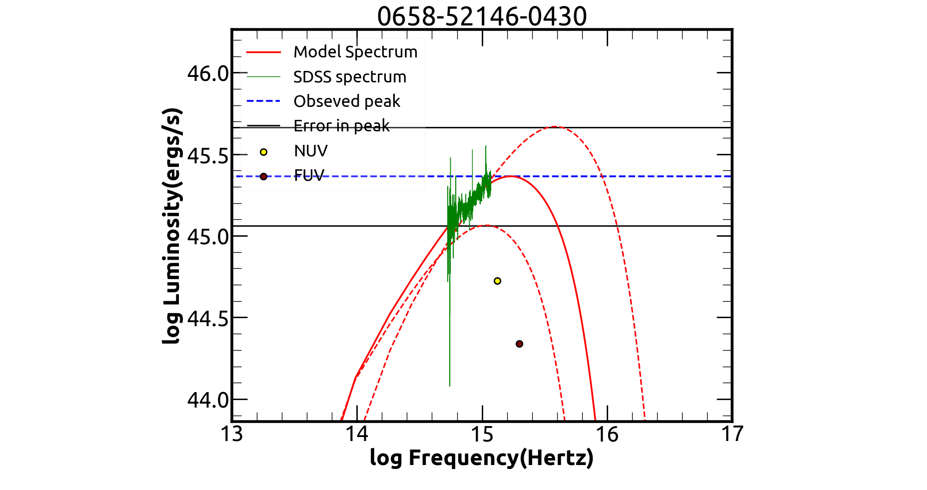
Figure 1: AD fits to the observed spectrum for two sources: 0658-52146-0430 (top panel), and 0785-52339-0007 (bottom panel). Here green is the observed SDSS spectrum, the red solid line is the calculated AD spectrum. The blue dashed line is the peak luminosity from the AD of the source derived from the H$\beta$ luminosity. The solid black lines are the 1 sigma error in the peak luminosity, that were used to estimate the error in M${}_{BH}^{AD}$. The filled circles are the GALEX measurements. They were not included in the fitting process.

3.2 M_BH using AD model fitting

Fitting Shakura-Sunyaev (S&S) AD model (Shakura & Sunyaev, 1973) to estimate M_BH is known and has been applied to type 1 AGN (Capellupo et al., 2015, 2016) and RL-NLS1s (Calderone et al., 2013). This technique is better than the virial M_BH method that is affected by uncertainties (Mejía-Restrepo et al., 2018) like (a) incomplete knowledge on the distribution of gas clouds (b) inclination of the AD to the line of sight and (c) dependence of the scale factor on inclination. For this work, we followed the procedure in Calderone et al. (2013) and described in brief below. We assumed a simple, non-relativistic, geometrically thin, optically thick AD in steady state, whose thermal emission is described by a standard S&S AD model. Each annulus of the AD emits black body radiation at a temperature, which is a function of radius R of the disk T(R), and the emitted spectrum is a superposition of several black body spectra. For evaluating the emitted spectrum the inner radius of the BH ($R_{in}$) was taken as 6$R_{g}$ and the outer radius as 2000$R_{g}$, where $R_{g}$ = G$M_{BH}$/$c^{2}$ is the gravitational radius of the BH. The radiative efficiency is $\eta$ = $R_{g}$/2$R_{in}$ and $M_{BH}^{AD}$ depends on both $R_{in}$ and $\eta$. The de-projection factor for calculating the isotropic disk luminosity was taken as $<2\cos\theta>=1.7$ corresponding to an average viewing angle ($\theta$) of $30^{\circ}$. The AD model created using the above assumptions varies with $M_{BH}^{AD}$, mass accretion rate $\dot{M}$ and $\eta$. The peak frequency ($\nu_{p}$) of the generated AD spectra and the luminosity at the peak frequency ($L_{\nu_{p}}$) scales as

$$\nu_{p}\propto\Big{(}\frac{\eta}{0.1}\Big{)}^{\nicefrac{{3}}{{4}}}\times\Big{(}\frac{M_{BH}^{AD}}{10^{6}M\textsubscript{$\odot$}}\Big{)}^{\nicefrac{{-1}}{{2}}}\times\Big{(}\frac{\dot{M}}{M\textsubscript{$\odot$}yr^{-1}}\Big{)}^{\nicefrac{{1}}{{4}}}$$ (3)

$$\nu_{p}{L_{\nu}}_{p}\propto\Big{(}\frac{\eta}{0.1}\Big{)}\times\Big{(}\frac{\dot{M}}{M\textsubscript{$\odot$}yr^{-1}}\Big{)}$$ (4)

For any given value of $\eta$, from an estimation of luminosity and $\nu_{p}$, the parameters $M_{BH}^{AD}$ and $\dot{M}$ can be determined. We obtained the isotropic disk luminosity using the sum of the broad and narrow component fluxes of $H\beta$ as:

$$L^{iso}_{d}(BLS1)=303\times L(H\beta)$$ (5)

$$L^{iso}_{d}(NLS1)=424\times L(H\beta)$$ (6)

where $L(H\beta)$ is the luminosity of the $H\beta$ line calculated from the derived fluxes using the procedures given in Rakshit et al. (2017). From the isotropic disk luminosity, we calculated the peak luminosity from the AD model as:

$$\nu_{p}L_{\nu_{p}}=0.5\times L^{iso}_{d}$$ (7)

This fixes a ’ceiling’ to the theoretical AD spectrum that was created. The error in H$\beta$ fluxes and the uncertainty of ${}_{\widetilde{~{}}}$2 in Equations 5 and 6 (Calderone et al., 2013), were propagated in the calculations to obtain an upper and lower limit to the peak disk luminosity $\nu_{p}L_{\nu_{p}}$.

The optical spectra for AD modeling were from SDSS DR-12. To avoid instrumental noise, we dropped bins equivalent to cover 110 Åfrom both the ends of each spectrum. The spectra were de-reddened following Cardelli et al. (1989) and brought to the rest frame. The contribution of the host galaxy to the observed spectra was removed following the procedure in Rakshit et al. (2017). Each of the resultant (de-reddened and host galaxy subtracted) spectrum was then matched with the generated theoretical AD spectrum.

The theoretical AD spectrum was first generated assuming an initial $M_{BH}^{AD}=5\times 10^{4}M\textsubscript{$\odot$}$, $\eta=0.1$ (fixed) and $\dot{M}=1.0M\textsubscript{$\odot$}yr^{-1}$ . The value of $\dot{M}$ was iteratively increased or decreased till the peak of the AD spectrum lies on the line defining the observed peak luminosity (shown as a blue dotted line in Figure 1) from the source. The value of $\dot{M}$ that gave the minimum $\chi^{2}$ between the peak of the AD spectrum and the line luminosity obtained via a fit of $\chi^{2}$ against $\dot{M}$ was considered as the final $\dot{M}$. Once this was achieved, $M_{BH}^{AD}$ was increased in steps of 5 $\times$ $10^{4}$ M_$\odot$. This shifts the theoretical AD spectrum horizontally. We chose two anchor points one around 2900 Å and the other around 3500 Å and evaluated $\chi^{2}$ at those two anchor points between the theoretical AD spectrum and the SDSS spectrum. This iteration was continued till we attained a minimum $\chi^{2}$ through a fit of $\chi^{2}$ against $M_{BH}^{AD}$. This constrains the BH mass of the source. The fitting was repeated for the upper and lower error limits of the peak disk luminosity (indicated by the solid black lines in Figure 1), to find the confidence limits in the estimated value of $M_{BH}^{AD}$.

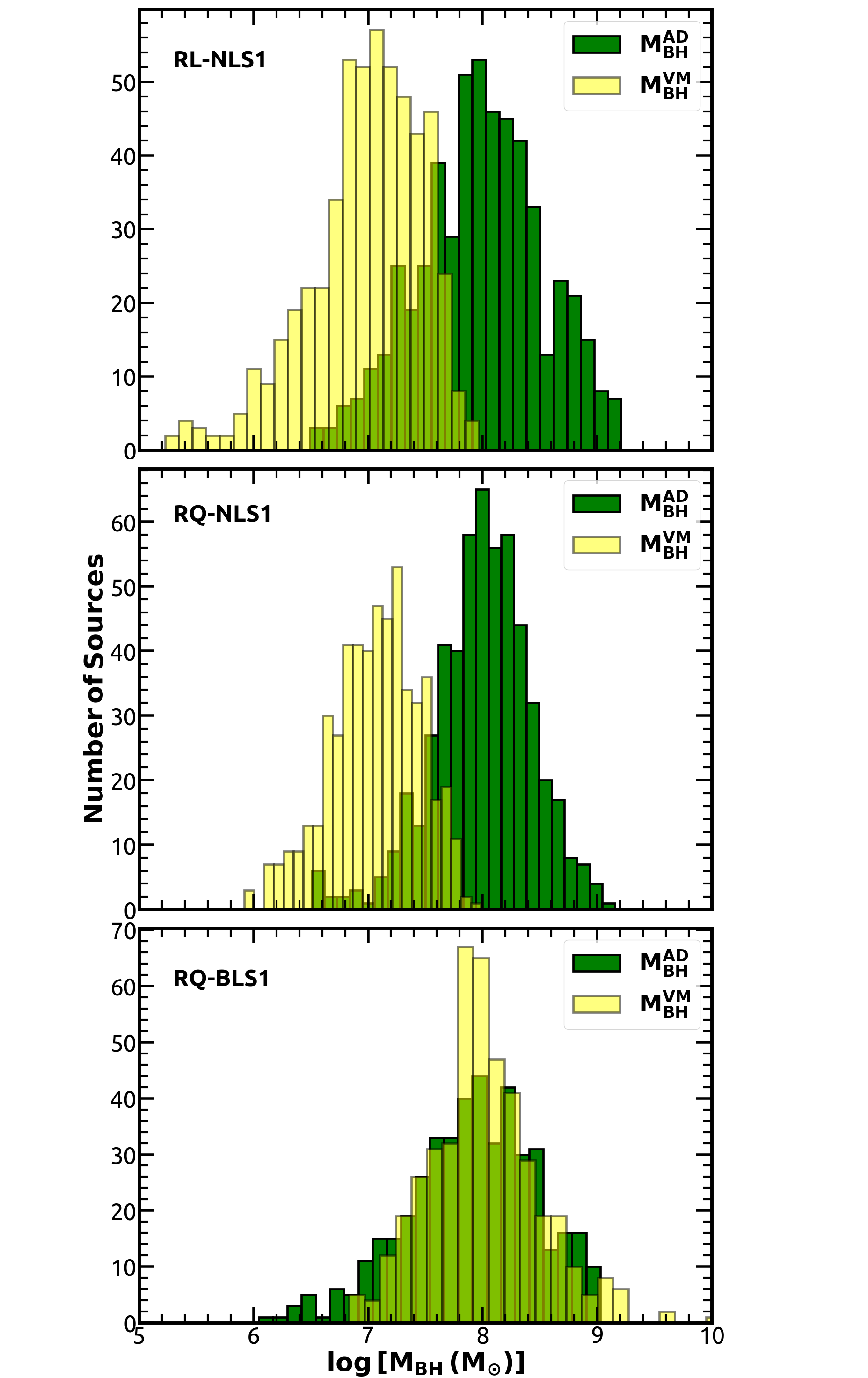
Figure 2: Distribution of logarithmic of M_BH in units of M_⊙ for different categories of sources in our sample. The yellow and green histograms are for M${}_{BH}^{VM}$ and $M_{BH}^{AD}$ respectively.

4 Results

4.1 M_BH of RL-NLS1s, RQ-NLS1s and BLS1s

The AD fitting was carried out on RL-NLS1s, RQ-NLS1s and RQ-BLS1s each consisting of 554 sources, except RQ-BLS1s that contain 471 sources. Of these, our automatic fitting procedure converged for 537 RL and RQ-NLS1s and 448 RQ-BLS1s. Spectral fits to two RL-NLS1s from our sample are shown in Figure 1 and the results are given in Table 1. In the same table are given M${}_{BH}^{VM}$ obtained for RQ-BLS1s using the VM outlined in Section 3.1 and taken from Rakshit et al. (2017) for NLS1s. Also given are the accretion rate ($\lambda_{Edd}$) calculated as $\lambda_{Edd}$ = $424\times L(H\beta)/L_{Edd}$ for NLS1s and $\lambda_{Edd}$ = $303\times L(H\beta)/L_{Edd}$ for BLS1s, where $L_{Edd}$ is the Eddington luminosity defined as $L_{Edd}=1.3\times 10^{38}\left(M_{BH}^{AD}/M_{\odot}\right)$ erg s^-1. For RQ-NLS1s, RL-NLS1s and RQ-BLS1s the calculated mean values of $\lambda_{Edd}$ are $0.06^{+0.16}_{-0.05}$, $0.05^{+0.18}_{-0.04}$ and $0.05^{+0.15}_{-0.04}$, respectively.

Table 1: Results of AD model fitting to the SDSS spectra. The table in full is available in the electronic version of the article .

$\alpha_{2000}$	$\delta_{2000}$	$z$	Type	R	log L(Hβ)	log($M_{BH}^{VM}/M_{\odot}$)	log($M_{BH}^{AD}/M_{\odot}$)	$\lambda_{Edd}$
					(ergs/s)
00:09:39.82	+13:27:17.0	0.482	RQ-NLS1	—-	41.75	6.82	7.57${}^{+0.61}_{-0.39}$	0.05${}^{+0.07}_{-0.04}$
00:08:04.17	-01:29:17.0	0.314	RL-NLS1	1.848	41.80	6.97	7.29${}^{+0.44}_{-0.35}$	0.11${}^{+0.13}_{-0.07}$
00:11:37.25	+14:42:01.4	0.132	RL-NLS1	0.711	41.93	7.16	7.69${}^{+0.47}_{-0.37}$	0.06${}^{+0.07}_{-0.04}$

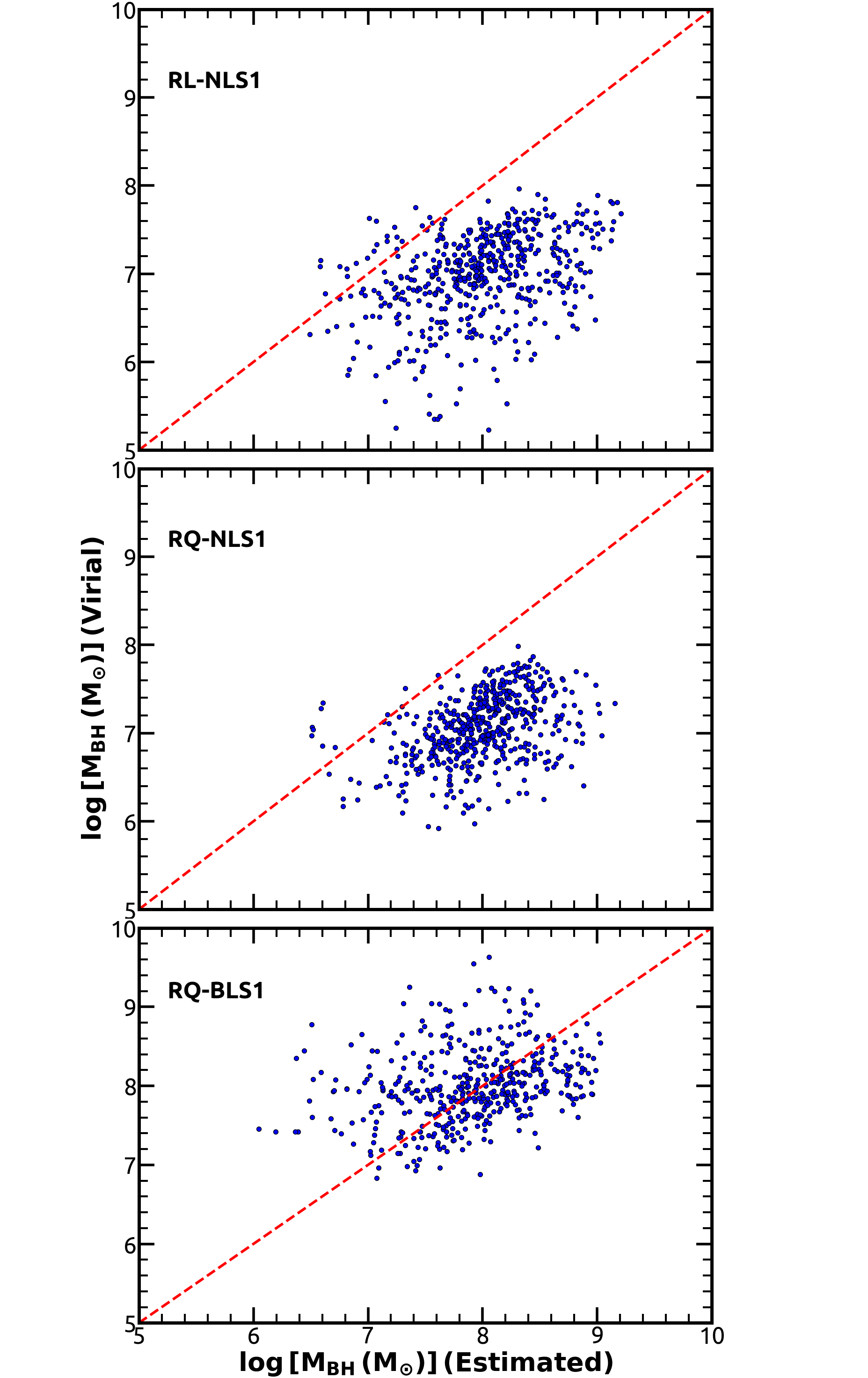
Figure 3: A comparison of the estimated M${}_{BH}^{VM}$ and M${}_{BH}^{AD}$ values for different categories of AGN. The red dashed line is for M${}_{BH}^{VM}$ = M${}_{BH}^{AD}$.

In Figure 2 (top panel) we show the distribution of $M_{BH}^{AD}$ and $M_{BH}^{VM}$ for RL-NLS1s. The mean value of log($\frac{M_{BH}^{AD}}{M\textsubscript{$\odot$}}$) is 7.98 $\pm$ 0.54. This is larger than the mean log($\frac{M_{BH}^{VM}}{M\textsubscript{$\odot$}}$) of 6.98 $\pm$ 0.49. A two sample Kolmogorov-Smirnov (KS) test at a significance of $\alpha$ = 5% confirms that the two distributions are different with a test statistics (D) of 0.70 and a null-hypothesis (the two distributions are identical) probability $p$ of 6.4 $\times$ 10^-116 . The distributions of $M_{BH}^{VM}$ and $M_{BH}^{AD}$ for RQ-NLS1s are shown in the middle panel of Figure 2. The two distributions are different with mean values of 7.07$\pm$0.38 and 8.00$\pm$0.43 for $M_{BH}^{VM}$ and $M_{BH}^{AD}$ respectively. This is confirmed by the KS test with D = 0.78 and p = 2.6 $\times$ 10^-146. The bottom panel of Figure 2 shows the distributions of $M_{BH}^{AD}$ and $M_{BH}^{VM}$ obtained for RQ-BLS1s. The distributions are nearly identical with mean values of 7.90$\pm$0.57 and 8.01$\pm$0.48 for $M_{BH}^{AD}$ and $M_{BH}^{VM}$ respectively. Though KS test rejects the null hypothesis with p=0.01, D has a small value of 0.11. Our analysis thus indicates that in both RL-NLS1s and RQ-NSL1s, $M_{BH}^{AD}$ values are systematically larger than $M_{BH}^{VM}$. However, in the case of RQ-BLS1s, both the estimates are not systematically different. This is evident from the plots in Figure 3. In the $M_{BH}^{AD}$ v/s $M_{BH}^{VM}$ diagram, for both RL-NLS1s and RQ-NLS1s the points are systematically away from the $M_{BH}^{AD}$ = $M_{BH}^{VM}$ line. In the case of RQ-BLS1s the points are scattered around the line, with the mean value of log($M_{BH}^{AD}$/$M_{BH}^{VM}$) = -0.11$\pm$0.64. For RL-NLS1s and RQ-NLS1s, we found mean log($M_{BH}^{AD}$/$M_{BH}^{VM}$) values of 1.00$\pm$0.57 and 0.93$\pm$0.45 respectively.

4.2 M_BH of $\gamma$-NLS1s

A total of 16 NLS1s are found to be emitters of $\gamma$-rays (Paliya et al., 2019). Of these, we have 9 $\gamma$-NLS1s in our sample. The values of M${}_{BH}^{AD}$ obtained for these 9 sources are given in Table 2. For these sources M${}_{BH}^{AD}$ values are larger that $M_{BH}^{VM}$ except one.

Table 2: Black hole masses of $\gamma$-NLS1s in our sample

$\alpha_{2000}$	$\delta_{2000}$	M${}_{BH}^{AD}$	M${}_{BH}^{VM}$
08:49:57.98	+51:08:29.1	7.86${}^{+0.64}_{-0.40}$	7.38
09:32:41.15	+53:06:33.8	8.01${}^{+0.53}_{-0.38}$	7.45
09:48:57.33	+00:22:25.5	8.97${}^{+0.01}_{-0.69}$	7.30
12:46:34.65	+02:38:09.1	8.63${}^{+0.27}_{-0.54}$	7.21
14:21:06.04	+38:55:22.8	8.63${}^{+0.30}_{-0.52}$	7.36
15:20:39.69	+42:11:11.2	7.07${}^{+0.35}_{-0.27}$	7.60
16:44:42.53	+26:19:13.3	8.30${}^{+0.46}_{-0.47}$	6.98
21:18:17.40	+00:13:16.8	7.98${}^{+0.78}_{-0.42}$	7.25
21:18:52.97	-07:32:27.6	7.94${}^{+0.78}_{-0.40}$	6.98

5 Discussion

It is likely that M${}_{BH}^{AD}$ values are close to the true BH masses in AGN, as this technique depends only on the ability to match the theoretical AD spectra to the observed SDSS spectra and is independent of the geometry and kinematics of the BLR (Mejía-Restrepo et al., 2018). The limitation here is the wavelength coverage of the SDSS spectra. Increased wavelength coverage into the UV region using data from GALEX could be an advantage, however we have not attempted here. This is because the SDSS spectra and the GALEX observations pertain to different epochs and our sources would have varied during those two epochs. Another important factor that can affect the M${}_{BH}^{AD}$ values is related to the contribution of relativistic jets to the SDSS spectra. This uncertainty will be there in the case of RL-NLS1s, however, unlikely to be present in RQ-NLS1s and RQ-BLS1s. We did not attempt to correct for this effect (see Calderone et al. 2013), firstly, because of the non-simultaneity of the infra-red measurements and SDSS spectra and secondly on the possibility of the sources in a faint activity state during the epoch when the SDSS spectra were taken leading to low/no contribution of jet emission to the spectra. Though AGN flux variability properties can in principle have some effect on AD model fits, they are unlikely to have any systematic effects on the estimated M${}_{BH}^{AD}$ values.

Though AD model fits to SDSS spectra to derive BH masses have the limitations described above, M${}_{BH}^{VM}$ estimation method too suffer from uncertainties like (i) lack of our knowledge on the geometry and kinematics of BLR and (ii) inclination of the source relative to the observer. From the $M_{BH}^{AD}$ values obtained for NLS1s, it is clear that our earlier knowledge of BH masses in them based on virial estimates is an underestimation. For our sample of 537 RL-NLS1s (that also includes 9 $\gamma$-NLS1s) we found mean log($M_{BH}^{AD}/M_{\odot}$) of 7.98$\pm$0.54. For our sample of RQ-NLS1s and RQ-BLS1s we found mean log($M_{BH}^{AD}/M_{\odot}$) values of 8.00$\pm$0.43 and 7.90$\pm$0.57 respectively. Thus our AD model fits to all the three categories of sources in a homogeneous manner point to similar BH masses in all the three categories. This leads us to conclude that NLS1s are not powered by low mass BHs, instead have BH masses similar to RQ-BLS1s and blazars. Report for large BH masses in NLS1s are available in literature from AD model fits (Calderone et al., 2013, 2018) and spectro-polarimetry (Baldi et al., 2016). Focussing only on the sub-set of 9 $\gamma$- NLS1s in our sample, we found mean log($M_{BH}^{AD}/M_{\odot}$) of 8.15$\pm$0.56. We are therefore inclined to argue that $\gamma$-NLS1s can no-longer be considered the “low mass BH counterparts to FSRQs”.

An explanation for the narrow width of broad emission lines in NLS1s and subsequently an underestimation of $M_{BH}^{VM}$ in them could be due to the assumption of these sources having a disk like BLR and viewed face on (Decarli et al., 2008). To probe the effects of viewing angle on the $M_{BH}^{AD}$ from AD fitting, we derived BH masses for the RL-NLS1s assuming a viewing angle of $\theta$ = $5^{\circ}$, which is typical of $\gamma$-ray emitting AGN. For RL-NLS1s we obtained mean log($M_{BH}^{AD}/M_{\odot}$) of 7.94 $\pm$ 0.54 which is similar to the mean log($M_{BH}^{AD}/M_{\odot}$) of 7.98 $\pm$ 0.54 obtained for the same sample considering a viewing angle of $30^{\circ}$. Therefore, AD model fits to the observed spectrum to find BH masses is less dependent on the viewing angle (see also Mejía-Restrepo et al. 2018). Also, Marconi et al. (2008) has proposed that the BH masses of NLS1s determined from optical spectroscopy can be underestimated when the radiation pressure from ionizing photons are neglected. In this work we have shown that the BH masses for the RQ-BLS1s obtained from AD model fitting is similar to that obtained from virial method. Therefore the method of AD model fits can be applied to find the BH masses of other AGN types.

This work clearly shows that NLS1s have BH masses and accretion rates similar to BLS1s and the BH masses of $\gamma$-NLS1s in our sample are similar to blazars. The only major difference that now persists between $\gamma$-NLS1s and FSRQs is related to their host galaxies. FSRQs are hosted by ellipticals and the scarce observations available on NLS1s point to ambiguity on their host galaxy type. NLS1s are preferentially hosted by spirals (Järvelä et al., 2018), but the hosts of some $\gamma$-NLS1s such as FBQS J1644+2619 and PKS 1502+036 seem to be elliptical (D’Ammando et al., 2017, 2018). If future deep imaging observations do confirm that $\gamma$-NLS1s are indeed hosted by spiral galaxies, launching of relativistic jets in AGN is independent of their host galaxy type. We do have reports of disk galaxies (Ledlow et al., 1998; Hota et al., 2011; Singh et al., 2015) as well as RL-NLS1s (see Rakshit et al. 2018 and references therein) having large scale relativistic jets.

6 Summary

1. We have estimated new BH masses using AD model fits and virial method for RQ-BLS1s, while for RQ-NLS1s and RL-NLS1s we have estimated new BH masses using AD model fits.

2. From AD model fits, the mean estimated values of log($M_{BH}^{AD}/M_{\odot}$) for RQ-NLS1s and RQ-BLS1s are 8.00$\pm$0.43 and 7.90$\pm$0.57, respectively. The corresponding mean values obtained from virial method are 7.07$\pm$0.38 and 8.01$\pm$0.48, respectively.

3. For RL-NLS1s and RQ-NLS1s we found that the BH masses estimated from AD model fits are about an order of magnitude times larger than the BH masses obtained from virial method. However, for RQ-BLS1s, the BH masses obtained from AD model fits are in reasonable agreement to that obtained from virial method with a mean difference of log($M_{BH}^{AD}/M_{BH}^{VM}$) = -0.11$\pm$0.64.

4. In our sample of 537 RL-NLS1s for which we were able to derive BH masses from AD fitting, 9 are emitters of $\gamma$-rays. The mean values of log(M${}_{BH}/M_{\odot}$) for these 9 sources from AD model fit and virial method are 8.15 $\pm$0.56 and 7.28 $\pm$ 0.20, respectively. This indicates that $\gamma$-ray emitting NLS1s are not low mass BH sources, instead have masses similar to blazars.

5. NLS1s are not low mass BH and highly accreting sources as believed now, instead have BH masses and accretion rates similar to BLS1s.

References

- Abdo et al. (2009) Abdo, A. A., Ackermann, M., Ajello, M., et al. 2009, ApJ, 699, 976
- Baldi et al. (2016) Baldi, R. D., Capetti, A., Robinson, A., Laor, A., & Behar, E. 2016, MNRAS, 458, L69
- Bentz et al. (2013) Bentz, M. C., Denney, K. D., Grier, C. J., et al. 2013, ApJ, 767, 149
- Boller et al. (1996) Boller, T., Brandt, W. N., & Fink, H. 1996, A&A, 305, 53
- Calderone et al. (2018) Calderone, G., D’Ammando, F., & Sbarrato, T. 2018, in Revisiting narrow-line Seyfert 1 galaxies and their place in the Universe. 9-13 April 2018. Padova Botanical Garden, Italy. Online at ¡A href=“https://pos.sissa.it/cgi-bin/reader/conf.cgi?confid=328”¿https://pos.sissa.it/cgi-bin/reader/conf.cgi?confid=328¡/A¿, id.44, 44
- Calderone et al. (2013) Calderone, G., Ghisellini, G., Colpi, M., & Dotti, M. 2013, MNRAS, 431, 210
- Capellupo et al. (2015) Capellupo, D. M., Netzer, H., Lira, P., Trakhtenbrot, B., & Mejía-Restrepo, J. 2015, MNRAS, 446, 3427
- Capellupo et al. (2016) —. 2016, MNRAS, 460, 212
- Cardelli et al. (1989) Cardelli, J. A., Clayton, G. C., & Mathis, J. S. 1989, ApJ, 345, 245
- Constantin & Shields (2003) Constantin, A., & Shields, J. C. 2003, PASP, 115, 592
- D’Ammando et al. (2018) D’Ammando, F., Acosta-Pulido, J. A., Capetti, A., et al. 2018, MNRAS, 478, L66
- D’Ammando et al. (2017) —. 2017, MNRAS, 469, L11
- D’Ammando et al. (2012) D’Ammando, F., Orienti, M., Finke, J., et al. 2012, MNRAS, 426, 317
- Decarli et al. (2008) Decarli, R., Dotti, M., Fontana, M., & Haardt, F. 2008, MNRAS, 386, L15
- Foschini (2011) Foschini, L. 2011, in Narrow-Line Seyfert 1 Galaxies and their Place in the Universe, 24
- Hota et al. (2011) Hota, A., Sirothia, S. K., Ohyama, Y., et al. 2011, MNRAS, 417, L36
- Järvelä et al. (2018) Järvelä, E., Lähteenmäki, A., & Berton, M. 2018, A&A, 619, A69
- Jiang et al. (2012) Jiang, N., Zhou, H.-Y., Ho, L. C., et al. 2012, ApJ, 759, L31
- Klimek et al. (2004) Klimek, E. S., Gaskell, C. M., & Hedrick, C. H. 2004, ApJ, 609, 69
- Komossa (2007) Komossa, S. 2007, in Astronomical Society of the Pacific Conference Series, Vol. 373, The Central Engine of Active Galactic Nuclei, ed. L. C. Ho & J.-W. Wang, 719
- Kshama et al. (2017) Kshama, S. K., Paliya, V. S., & Stalin, C. S. 2017, MNRAS, 466, 2679
- Lähteenmäki et al. (2017) Lähteenmäki, A., Järvelä, E., Hovatta, T., et al. 2017, A&A, 603, A100
- Ledlow et al. (1998) Ledlow, M. J., Owen, F. N., & Keel, W. C. 1998, ApJ, 495, 227
- Leighly (1999) Leighly, K. M. 1999, ApJS, 125, 317
- Marconi et al. (2008) Marconi, A., Axon, D. J., Maiolino, R., et al. 2008, ApJ, 678, 693
- Mejía-Restrepo et al. (2018) Mejía-Restrepo, J. E., Lira, P., Netzer, H., Trakhtenbrot, B., & Capellupo, D. M. 2018, Nature Astronomy, 2, 63
- Moran et al. (1996) Moran, E. C., Halpern, J. P., & Helfand, D. J. 1996, ApJS, 106, 341
- Ojha et al. (2019) Ojha, V., Krishna, G., & Chand, H. 2019, MNRAS, 483, 3036
- Osterbrock & Pogge (1985) Osterbrock, D. E., & Pogge, R. W. 1985, ApJ, 297, 166
- Paliya et al. (2018) Paliya, V. S., Ajello, M., Rakshit, S., et al. 2018, ApJ, 853, L2
- Paliya et al. (2019) Paliya, V. S., Parker, M. L., Jiang, J., et al. 2019, ApJ, 872, 169
- Paliya et al. (2016) Paliya, V. S., Rajput, B., Stalin, C. S., & Pandey, S. B. 2016, ApJ, 819, 121
- Paliya et al. (2014) Paliya, V. S., Sahayanathan, S., Parker, M. L., et al. 2014, ApJ, 789, 143
- Paliya et al. (2013) Paliya, V. S., Stalin, C. S., Kumar, B., et al. 2013, MNRAS, 428, 2450
- Rakshit et al. (2019) Rakshit, S., Johnson, A., Stalin, C. S., Gandhi, P., & Hoenig, S. 2019, MNRAS, 483, 2362
- Rakshit & Stalin (2017) Rakshit, S., & Stalin, C. S. 2017, ApJ, 842, 96
- Rakshit et al. (2017) Rakshit, S., Stalin, C. S., Chand, H., & Zhang, X.-G. 2017, ApJS, 229, 39
- Rakshit et al. (2018) Rakshit, S., Stalin, C. S., Hota, A., & Konar, C. 2018, ApJ, 869, 173
- Rani et al. (2017) Rani, P., Stalin, C. S., & Rakshit, S. 2017, MNRAS, 466, 3309
- Rodriguez-Pascual et al. (1997) Rodriguez-Pascual, P. M., Mas-Hesse, J. M., & Santos-Lleo, M. 1997, A&A, 327, 72
- Ryan et al. (2007) Ryan, C. J., De Robertis, M. M., Virani, S., Laor, A., & Dawson, P. C. 2007, ApJ, 654, 799
- Shakura & Sunyaev (1973) Shakura, N. I., & Sunyaev, R. A. 1973, A&A, 24, 337
- Singh et al. (2015) Singh, V., Ishwara-Chandra, C. H., Sievers, J., et al. 2015, MNRAS, 454, 1556
- Wang et al. (1996) Wang, T., Brinkmann, W., & Bergeron, J. 1996, A&A, 309, 81
- Williams et al. (2018) Williams, J. K., Gliozzi, M., & Rudzinsky, R. V. 2018, MNRAS, 480, 96
- Yang et al. (2018) Yang, H., Yuan, W., Yao, S., et al. 2018, ArXiv e-prints, arXiv:1801.03963
- Yuan et al. (2008) Yuan, W., Zhou, H. Y., Komossa, S., et al. 2008, ApJ, 685, 801
- Zhou et al. (2006) Zhou, H., Wang, T., Yuan, W., et al. 2006, ApJS, 166, 128