Fair Integral Network Flows

Abstract

A strongly polynomial algorithm is developed for finding an integer-valued feasible $st$-flow of given flow-amount which is decreasingly minimal on a specified subset $F$ of edges in the sense that the largest flow-value on $F$ is as small as possible, within this, the second largest flow-value on $F$ is as small as possible, within this, the third largest flow-value on $F$ is as small as possible, and so on. A characterization of the set of these $st$-flows gives rise to an algorithm to compute a cheapest $F$-decreasingly minimal integer-valued feasible $st$-flow of given flow-amount. Decreasing minimality is a possible formal way to capture the intuitive notion of fairness.

Keywords:  Lexicographic minimization, Network flow, Polynomial algorithm.

Mathematics Subject Classification (2010): 90C27, 05C, 68R10

1 Introduction

In optimization problems, a typical task is to find an extreme element of a set $Q$ of ‘feasible’ vectors, where extreme means that we maximize (or minimize) a certain (linear or more general) objective function. A different (though related) concept in optimization is when one is interested in finding an element of $Q$ whose components are distributed in a way which is felt the most uniform (fair, equitable, egalitarian). The term ‘fair’ in the title of this paper refers to the intuitive meaning of the word. There may be various formal definitions for capturing this intuitive feeling. For example, if the square-sum of the components is minimal, then the distribution of the components is felt rather fair. Another possible way to formally capture fairness is to minimize the sum of the absolute values of the pairwise differences of the components. A third possibility is lexicographic minimization. These definitions are equivalent in some cases while they are different in other situations. We should emphasize that the ‘fairness’ concept shows up in the literature in the most diverse contexts (such as fair resource allocation in operations research [21, 23], fair division of goods in economics [26, 29], load balancing in computer networks [15, 18], etc.). In the present work, however, fairness will be formulated into the concept of ‘decreasing minimality’ (see, below).

An early example of a possible fairness concept is due to N. Megiddo [24, 25], who introduced and solved the problem of finding a (possibly fractional) maximum flow which is ‘lexicographically optimal’ on the set of edges leaving the source node. The problem, in equivalent terms, is as follows. Let $D=(V,A)$ be a digraph with a source-node $s$ and a sink-node $t$, and let $S_{A}$ denote the set of edges leaving $s$. We assume that no edge enters $s$ and no edge leaves $t$. Let $g:A\rightarrow{\bf R}_{+}$ be a non-negative capacity function on the edge-set. By the standard definition, an $st$-flow, or just a flow, is a function $x:A\rightarrow{\bf R}_{+}$ for which $\varrho_{x}(v)=\delta_{x}(v)$ holds for every node $v\in V-\{s,t\}$. (Here $\varrho_{x}(v):=\sum[x(uv):uv\in A]$ and $\delta_{x}(v):=\sum[x(vu):vu\in A]$.) The flow is called feasible if $x\leq g$. The flow-amount of $x$ is $\delta_{x}(s)$ which is equal to $\varrho_{x}(t)$. We refer to a feasible flow with maximum flow-amount as a max-flow.

Megiddo solved the problem of finding a feasible flow $x$ which is lexicographically optimal on $S_{A}$ in the sense that the smallest $x$-value on $S_{A}$ is as large as possible, within this, the second smallest (though not necessarily distinct) $x$-value on $S_{A}$ is as large as possible, and so on. It is a known fact (implied, for example, by the max-flow algorithm of Ford and Fulkerson [6]) that a lexicographically optimal flow is a max-flow. It is a basic property of flows that for an integral capacity function $g$ there always exists a max-flow which is integer-valued. On the other hand, an easy example [10] shows that even when $g$ is integer-valued, the unique max-flow that is lexicographically optimal on $S_{A}$ may not be integer-valued.

A member $x$ of a set $Q$ of vectors is called a decreasingly minimal (dec-min, for short) element of $Q$ if the largest component of $x$ is as small as possible, within this, the next largest (but not necessarily distinct) component of $x$ is as small as possible, and so on. The term ‘decreasing minimality’ was introduced in [10, 11] as one of the possible formulations of the intuitive notion of fairness. Analogously, $x$ is an increasingly maximal (inc-max) element of $Q$ if its smallest component is as large as possible, within this, the next smallest component of $x$ is as large as possible, and so on. Therefore increasing maximality is the same as Megiddo’s lexicographic optimality and ‘lexmin optimality’ of Plaut and Roughgarden [29], whereas the notion of co-lexicographic optimality, introduced in Fujishige [14, page 264], is the same as decreasing minimality. In general, a dec-min element is not necessarily inc-max, and an inc-max element is not necessarily dec-min. However, in Megiddo’s problem where $Q$ is the restriction of a feasible maximum flow to $S_{A}$, it is known that an element of $Q$ is dec-min if and only if it is inc-max. Fujishige [13, 14] proved that this equivalence is still true in a more general setting where $Q$ is a base-polyhedron [14, 27]. He also proved that the (unique) dec-min element of $Q$ is the (unique) square-sum minimizer of $Q$.

In [10] and [11], the present authors solved the discrete counterpart of Megiddo’s problem when the capacity function $g$ is integral and one is interested in finding an integral max-flow whose restriction to the set $S_{A}$ of edges leaving $s$ is increasingly maximal. This was actually a consequence of the more general result concerning dec-min elements of an M-convex set (where an M-convex set [27], by definition, is the set of integral elements of an integral base-polyhedron). Among others, it was proved that an element $z$ is decreasingly minimal if and only if $z$ is increasingly maximal. It was also proved in [10] that an element $z$ of an M-convex set is dec-min if and only if $z$ is square-sum minimizer. A strongly polynomial algorithm was also developed for finding a dec-min element. Since the restrictions of max-flows to $S_{A}$ form a base-polyhedron, this gives an algorithm to find an integral max-flow which is decreasingly minimal (and increasingly maximal) when restricted to $S_{A}$.

A closely related previous work is due to Kaibel, Onn, and Sarrabezolles [22]. They considered (in an equivalent formulation) the problem of finding an integer-valued uncapacitated $st$-flow with specified flow-amount $K$ which is decreasingly minimal on the whole edge-set $A$. They developed an algorithm which is polynomial in the size of digraph $D=(V,A)$ plus the value of $K$ but is not polynomial in the size of number $K$ (which is roughly $\lceil\log K\rceil$). This is analogous to the well-known characteristic of the classic Ford–Fulkerson max-flow algorithm [6], where the running time is proportional to the largest value $g_{\max}$ of the capacity function $g$, and therefore this algorithm is not polynomial (unless $g_{\max}$ is small in the sense that it is bounded by a polynomial of $|A|$). It should also be mentioned that Kaibel et al. considered exclusively the uncapacitated $st$-flow problem, where no capacity (upper-bound) restrictions are imposed on the edges. (For example, the flow-value on any edge is allowed to be $K$.)

In the present work, we consider the more general question when $F\subseteq A$ is an arbitrarily specified subset of edges, and we are interested in finding a feasible integral max-flow whose restriction to $F$ is decreasingly minimal. This problem substantially differs from its special case with $F=S_{A}$ mentioned above in that the set of restrictions of max-flows to $F$ is not necessarily a base-polyhedron. The significant difference is nicely demonstrated by the fact that an element $z$ of an M-convex set, as mentioned earlier, is dec-min if and only if it is inc-max if and only if it is a square-sum minimizer, whereas these three criteria are (pairwise) different for integral feasible network flows (see Section 11.2). In this light, it is not surprising that the dec-min problem for integral network flows is much harder than for M-convex sets.

We emphasize the fundamental difference between fractional and integral dec-min flows. Figure 1 demonstrates this difference for a simple example, where all edges have a unit capacity ($g\equiv 1$) and dec-min unit flows from $s$ to $t$ are considered for $F=A$ (all edges). Whereas the dec-min fractional flow is uniquely determined, there are two dec-min integral flows.

As the theory of network flows has a multitude of applications, the algorithm presented in this paper may also be useful in these special cases. For example, the paper by Harvey, Ladner, Lovász, and Tamir [18] considered the problem of finding a subgraph of a bipartite graph $G=(S,T;E)$ for which the degree-sequence in $S$ is identically 1 and the degree-sequence in $T$ is decreasingly minimal. This problem was extended to a more general setting (see [11]) but the following version needs the present general flow approach: Find a subgraph of $G=(S,T;E)$ of $\gamma$ edges for which the degree-sequence on the whole node-set $S\cup T$ (or on an arbitrarily specified subset of $S\cup T$) is decreasingly minimal.

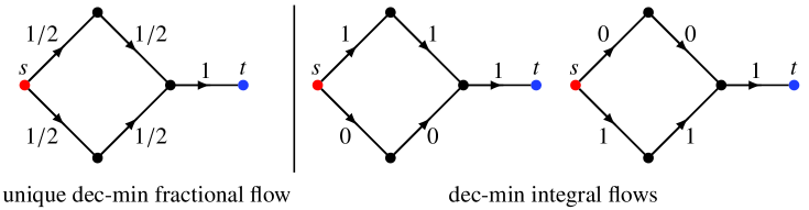
Figure 1: Difference between fractional and integral dec-min flows

Our main goal is to provide a description of the set of integral max-flows which are dec-min on $F$ as well as a strongly polynomial algorithm to find such a max-flow. The description makes it possible to solve algorithmically even the minimum cost dec-min max-flow problem. Instead of maximum $st$-flows, we consider the formally more general (though equivalent) setting of modular flows which, however, allows a technically simpler discussion.

It is quite natural to consider the dec-min problem over the intersection of two M-convex sets, which is called an M₂-convex set in the literature [27]. This problem is much harder than the dec-min problem over an M-convex set. The relationship of the difficulties is similar to that between the classic problems of finding a maximum weight basis of a matroid and finding a maximum weight common basis of two matroids (or more generally, between a maximum weight element of an M-convex set and of an M₂-convex set). An even more general framework is the set of integral submodular flows, introduced by Edmonds and Giles [4], which includes both standard integral network flows ($m$-flows) and M₂-convex sets. In [12], we have worked out a strongly polynomial algorithm for finding an integral dec-min submodular flow.

The paper is organized as follows. In Section 2, after introducing the basic definitions, we formulate Theorem 2.1 which is the main theoretical result of the paper. This is proved in Section 5 after the necessary structural results are developed in Sections 3 and 4. An important consequence of the characterization in Theorem 2.1 is that it makes possible to manage algorithmically even the minimum edge-cost version of the integral dec-min flow problem. Section 6 provides an alternative characterization of $F$-dec-min integral feasible flows by developing extensions of such standard concepts from network optimization as improving di-circuits and feasible potentials. Section 7 provides a necessary and sufficient condition for the existence of an integral $F$-dec-min flow. Sections 8–10 are devoted to algorithmic aspects. Sections 8 and 9 describe strongly polynomial algorithms for each component, and Section 10 shows how these components are synthesized. Finally, in the supplementary Section 11 of the paper, we briefly outline two closely related topics: fractional dec-min flows and the relation to convex minimization over flows.

2 Decreasingly-minimal integer-valued feasible modular flows

2.1 Modular flows

Let $D=(V,A)$ be a digraph endowed with integer-valued functions $f:A\rightarrow{\bf Z}\cup\{-\infty\}$ and $g:A\rightarrow{\bf Z}\cup\{+\infty\}$ for which $f\leq g$. Here $f$ and $g$ are serving as lower and upper bound functions, respectively. An edge $e$ is called $(f,g)$-tight or just tight if $f(e)=g(e)$. The polyhedron $T(f,g):=\{x:f\leq x\leq g\}$ is called a box.

We are given a finite integer-valued function $m$ on $V$ for which $\widetilde{m}(V)=0$. (Here and throughout, $\widetilde{m}(X):=\sum[m(v):v\in X]$.) A modular flow (with respect to $m$) or, for short, a mod-flow $x$ is a finite-valued function on $A$ (or a vector in ${\bf R}^{A}$) for which $\varrho_{x}(v)-\delta_{x}(v)=m(v)$ for each node $v\in V$. When we want to emphasize the defining vector $m$, we speak of an $m$-flow.

A mod-flow $x$ is called $(f,g)$-bounded or feasible if $f\leq x\leq g$. A circulation is an $m$-flow with respect to $m\equiv 0$, and an $st$-flow of given flow-amount $K$ is also an $m$-flow with respect to $m$ defined by

$$m(v):=\begin{cases}0&\ \ \hbox{if}\ \ \ v\in V-\{s,t\},\cr K&\ \ \hbox{if}\ \ \ v=t,\cr-K&\ \ \hbox{if}\ \ \ v=s.\end{cases}$$ (2.1)

Circulations form a subspace of ${\bf R}^{A}$ while the set of mod-flows is an affine space. The set of feasible mod-flows, which is called a feasible mod-flow polyhedron, may be viewed as the intersection of this affine subspace with the box $T(f,g)$. It follows from this definition that the face of such a polyhedron is also a feasible $m$-flow polyhedron. We note, however, that the projection along axes is not necessarily a feasible mod-flow polyhedron since its description may need an exponential number of inequalities while a feasible mod-flow polyhedron is described by at most $2|A|+|V|$ inequalities.

Let $Q=Q(f,g;m)$ denote the set of $(f,g)$-bounded $m$-flows. Hoffman’s theorem [20] states that $Q$ is non-empty if and only if the Hoffman-condition $\varrho_{g}-\delta_{f}\geq\widetilde{m}$ holds, that is,

$$\varrho_{g}(Z)-\delta_{f}(Z)\geq\widetilde{m}(Z)\quad\hbox{for every}\ \ \ Z\subseteq V.$$ (2.2)

It is well-known that $Q$ is an integral polyhedron whenever $f$, $g$, and $m$ are integral vectors. In the integral case let $\overset{....}{Q}=\overset{....}{Q}(f,g;m)$ denote the set of integral elements of $Q$, that is,

$$\overset{....}{Q}:=Q\cap{\bf Z}^{A}.$$ (2.3)

In Section 1 we introduced (the basic form of) the notion of decreasing minimality, but we actually work with the following slightly extended definition. Let $F$ be a specified subset of $A$. We say that $z\in\overset{....}{Q}(f,g;m)$ is decreasingly minimal on $F$ (or $F$-dec-min for short) if the restriction of $z$ to $F$ is decreasingly minimal among the restrictions of the vectors in $\overset{....}{Q}(f,g;m)$ to $F$.

Our first main goal is to prove the following characterization of the subset of elements of $\overset{....}{Q}$ which are decreasingly minimal on $F$.

Theorem 2.1.

Let $D=(V,A)$ be a digraph endowed with integer-valued lower and upper bound functions $f:A\rightarrow{\bf Z}\cup\{-\infty\}$ and $g:A\rightarrow{\bf Z}\cup\{+\infty\}$ for which $f\leq g$. Let $m:V\rightarrow{\bf Z}$ be a function on $V$ with $\widetilde{m}(V)=0$ such that there exists an $(f,g)$-bounded $m$-flow. Let $F\subseteq A$ be a specified subset of edges such that both $f$ and $g$ are finite-valued on $F$. There exists a pair $(f^{*},g^{*})$ of integer-valued functions on $A$ with $f\leq f^{*}\leq g^{*}\leq g$ (allowing $f^{*}(e)=-\infty$ and $g^{*}(e)=+\infty$ for $e\in A-F$) such that an integral $(f,g)$-bounded $m$-flow $z$ is decreasingly minimal on $F$ if and only if $z$ is an integral $(f^{*},g^{*})$-bounded $m$-flow. Moreover, the box $T(f^{*},g^{*})$ is narrow on $F$ in the sense that $0\leq g^{*}(e)-f^{*}(e)\leq 1$ for every $e\in F$.  

Our second main goal is to describe a strongly polynomial algorithm to compute $f^{*}$ and $g^{*}$. Once these bounds are available, one is able to compute not only a single $(f,g)$-bounded integer-valued $m$-flow which is dec-min on $F$ but a minimum cost $F$-dec-min $m$-flow as well (with the help of a standard min-cost circulation algorithm). Section 10 summarizes what the various components of the whole algorithm aim at and how these components are related to each other.

Remark 2.1.

In Section 7, we shall consider the general case when $f$ and $g$ are not required to be finite-valued on $F$. In this case, an $F$-dec-min $(f,g)$-feasible $m$-flow may not exist, and we shall provide a characterization for the existence. In Theorem 7.6, we shall show how Theorem 2.1 can be extended to the case when only the existence of an $F$-dec-min $(f,g)$-feasible $m$-flow is assumed.  

Remark 2.2.

One may also be interested in finding an (integral) $(f,g)$-bounded $m$-flow $z$ which is increasingly maximal (inc-max) on $F$ in the sense that the smallest $z$-value on $F$ is as large as possible, within this, the second smallest (but not necessarily distinct) $z$-value on $F$ is as large as possible, and so on. (Megiddo [24], [25], for example, considered the fractional inc-max problem for $st$-flows when $F$ was the set of edges leaving $s$.) But an $(f,g)$-bounded $m$-flow $z$ is increasingly maximal on $F$ precisely if $-z$ is a $(-g,-f)$-bounded $(-m)$-flow which is dec-min on $F$, implying that the inc-max and the dec-min problems are equivalent for modular flows. Hence we concentrate throughout only on decreasing minimality. Note that in [10] we investigated these problems for M-convex sets and proved that the two problems are not only equivalent but they are one and the same in the sense that an element $z$ of an M-convex set is dec-min if and only if $z$ is inc-max. (As mentioned earlier, an M-convex set, by definition, is nothing but the set of integral elements of an integral base-polyhedron).  

Remark 2.3.

It is well-known that there are strongly polynomial algorithms that find a feasible $m$-flow when it exists or find a subset $Z$ violating (2.2) (see, for example, appropriate variations of the algorithms by Edmonds and Karp [5], Dinits [3], or Goldberg and Tarjan [17]). Actually, when no feasible $m$-flow exists, not only a violating subset can be computed but the most violating set as well, that is, a set $Z^{*}$ maximizing $\widetilde{m}(Z)-\varrho_{g}(Z)+\delta_{f}(Z)$. Note that this latter function is fully supermodular (see (3.1) for definition), and there is a general algorithm to maximize an arbitrary supermodular function. The point here is that for finding $Z^{*}$ we do not have to rely on this general algorithm since much simpler (and more efficient) flow-techniques do the job.  

2.2 Approach of the proof of Theorem 2.1

By tightening an edge $e$ we mean the operation that replaces the bounding pair $(f(e),g(e))$ by $(f^{\prime}(e),g^{\prime}(e))$ where $f(e)\leq f^{\prime}(e)\leq g^{\prime}(e)\leq g(e)$ and $g^{\prime}(e)-f^{\prime}(e)<g(e)-f(e)$. Note that tightening an edge does not necessarily make the edge tight. The approach of the proof is that we tighten edges as long as possible without loosing any integral $m$-flow which is dec-min on $F$, and prove that when no more tightening step is available for the current $(f^{*},g^{*})$ then every $(f^{*},g^{*})$-bounded integral $m$-flow is an $F$-dec-min element of $\overset{....}{Q}(f,g;m)$.

A natural reduction step consists of removing a tight edge $e$ from $F$ (where $e$ could be tight originally or may have become tight during a tightening step). This simply means that we replace $F$ by $F^{\prime}:=F-e$ (but keep $e$ in the digraph itself). Obviously, an $m$-flow $z$ is $F$-dec-min if and only if $z$ is $F^{\prime}$-dec-min. Therefore, we may always assume that $F$ contains no tight edges.

We say that an integral $(f,g)$-bounded $m$-flow $z$ is an $F$-max minimizer if the largest component of $z$ in $F$ is as small as possible. Clearly, every $F$-dec-min $m$-flow $z\in\overset{....}{Q}(f,g;m)$ is $F$-max minimizer. Let $\beta_{F}$ denote this smallest maximum value, that is,

$$\beta_{F}:=\min\{\max\{z(a):a\in F\}:z\in\overset{....}{Q}(f,g;m)\}.$$ (2.4)

Note that $\beta_{F}$ may be interpreted as the smallest integer for which there is an integer-valued feasible $m$-flow after decreasing $g(e)$ to $\beta_{F}$ for each $e\in F$ with $g(e)>\beta_{F}$. In Section 9, we shall describe how $\beta_{F}$ can be computed in strongly polynomial time with the help of a discrete variant of the Newton–Dinkelbach algorithm and a standard max-flow algorithm, but for the proof of Theorem 2.1 we assume that $\beta_{F}$ is available. Therefore, we can assume that $\max\{g(e):e\in F\}=\beta_{F}$ which is equivalent to requiring that $Q(f,g;m)$ is non-empty but $Q(f,g^{-};m)=\emptyset$ where $g^{-}$ arises from $g$ by subtracting 1 from $g(e)$ for each $e\in F$ with $g(e)=\beta_{F}$.

3 Covering a supermodular function by a smallest subgraph

A family of subsets is called laminar if one of $X\subseteq Y$, $Y\subseteq X$, $X\cap Y=\emptyset$ holds for every pair of its members. We say that a digraph $D=(V,A)$ (or its edge-set $A$) covers a set-function $p$ if $\varrho_{D}(Z)\geq p(Z)$ for every subset $Z\subseteq V$, where $\varrho_{D}$ is the in-degree function of $D$. A set-function $p$ is called fully supermodular or just supermodular if the supermodular inequality

$$p(X)+p(Y)\leq p(X\cap Y)+p(X\cup Y)$$ (3.1)

holds for every pair of subsets $X$ and $Y$. When this inequality required only for intersecting pairs (that is, when $X\cap Y\neq\emptyset$), then we speak of an intersecting supermodular function [8].

Let $p:2^{V}\rightarrow{\bf Z}\cup\{-\infty\}$ be an intersecting supermodular set-function on $V$ and let $D_{L}=(V,L)$ be a digraph covering $p$. We are interested in the minimum cardinality subset of edges of $D_{L}$ that covers $p$. Let $A_{L}$ denote the $(0,1)$-matrix whose rows correspond to subsets $X$ of $V$ for which $p(X)>-\infty$ and the columns correspond to the edges in $L$. An entry of $A_{L}$ corresponding to $Z$ and $e$ is 1 if $e$ enters $Z$ and 0 otherwise. The following result was proved in [7] (see, also, Theorem 17.1.1 in the book [8]).

Theorem 3.1.

Let $p$ be an intersecting supermodular set-function on $V$. The linear inequality system $[A_{L}x_{L}\geq p,\ x_{L}\leq\underline{1},\ x_{L}\geq 0]$ is totally dual integral (TDI). (Hence) the primal linear program

$$\min\{\underline{1}x_{L}:\ A_{L}x_{L}\geq p,\ x_{L}\leq\underline{1},\ x_{L}\geq 0\}$$ (3.2)

and the dual linear program

$$\max\{yp-\underline{1}z:yA_{L}-z\leq\underline{1},\ (y,z)\geq 0\}$$ (3.3)

have integer-valued optimal solutions, where $\underline{1}$ denotes the everywhere 1 vector of dimension $|L|$. Moreover, there is an integer-valued dual optimum $(y^{*},z^{*})$ for which its support family ${\cal L}:=\{Z:y^{*}(Z)>0\}$ is laminar.  

For a family $\cal L$ of subsets of $V$, let $\varrho_{L}({\cal L})$ denote the number of edges entering at least one member of $\cal L$. The min-max theorem arising from Theorem 3.1 is as follows.

Theorem 3.2.

Given a digraph $D_{L}=(V,L)$ covering an intersecting supermodular function $p$, the minimum number of edges of $D_{L}$ covering $p$ is equal to

$$\max\{\varrho_{L}({\cal L})\ -\sum[\varrho_{L}(Z)-p(Z):\ Z\in{\cal L}]\ \},$$ (3.4)

where the maximum is taken over all laminar families $\cal L$ of subsets $Z$ of $V$ with $p(Z)>-\infty$. When $p$ is fully supermodular, the optimal laminar family ${\cal L}^{*}$ may be chosen as a chain of subsets $V_{1}\supset V_{2}\supset\cdots\supset V_{q}$ of $V$.

Proof. Suppose that we remove some edges from $L$ so that the set $X$ of the remaining edges continues to cover $p$. For each $Z\in{\cal L}$, the number of removed edges entering $Z$ is bounded by $\varrho_{L}(Z)-p(Z)$, and hence the number of removed edges entering at least one member of $\cal L$ is bounded from above by $\sum[\varrho_{L}(Z)-p(Z):Z\in{\cal L}]$. On the other hand, the number of removed edges entering at least one member of $\cal L$ is bounded from below by $\varrho_{L}({\cal L})-|X|$. Therefore we have

$$\varrho_{L}({\cal L})-|X|\leq\sum[\varrho_{L}(Z)-p(Z):Z\in{\cal L}],$$

from which the trivial direction $\max\leq\min$ follows.

To see the reverse inequality, we have to find a covering $X^{*}\subseteq L$ of $p$ and a laminar family ${\cal L}^{*}$ for which equality holds. To this end, let $x^{*}$ be a $(0,1)$-valued optimal solution of the primal problem (3.2) in Theorem 3.1 and let $(y^{*},z^{*})$ be an integer-valued optimal solution of the dual problem for which its support family ${\cal L}^{*}$ is laminar. Then the subset $X^{*}:=\{e\in L:x^{*}(e)=1\}$ is a smallest subset of $L$ covering $p$.

Observe that $y^{*}$ uniquely determines $z^{*}$, namely, $z^{*}(e)=0$ when $e$ enters no member of  ${\cal L}^{*}$ and

$$z^{*}(e)=\sum[y^{*}(Z):Z\in{\cal L}^{*},e\ \hbox{enters}\ \ Z]\ -1$$ (3.5)

when $e$ enters at least one member of ${\cal L}^{*}$.

Claim 3.3.

The optimal $y^{*}$ may be chosen $(0,1)$-valued.

Proof. Suppose that $(y^{*},z^{*})$ is an integer-valued dual optimum in which the sum of $y^{*}$-components is as small as possible. We show that $y^{*}$ is $(0,1)$-valued. Suppose indirectly that $y^{*}(Z)\geq 2$ for some set $Z$. In this case $z^{*}(e)\geq 1$ for every edge $e$ entering $Z$. If we decrease $y^{*}(Z)$ by 1 and decrease $z^{*}(e)$ by 1 on every edge $e$ entering $Z$, then the resulting $(y^{\prime},z^{\prime})$ is also a dual feasible solution for which

$$y^{*}p-\underline{1}z^{*}\ \geq\ y^{\prime}p-\underline{1}z^{\prime}\ =\ y^{*}p-\underline{1}z^{*}-p(Z)+\varrho_{L}(Z)\ \geq\ y^{*}p-\underline{1}z^{*},$$

where the last inequality follows from the assumption that $D_{L}$ covers $p$ and hence $\varrho_{L}(Z)\geq p(Z)$. Therefore we have equality throughout and hence $(y^{\prime},z^{\prime})$ is also an optimal dual solution, contradicting the minimal choice of $y^{*}$. Thus Claim 3.3 is proved.  

By the claim, (3.5) simplifies as follows:

$$z^{*}(e)=\hbox{$[$the number of members of $\cal L$ entered by $e]\ -1.$}\$$ (3.6)

Now the dual optimum value is:

$$y^{*}p-\underline{1}z^{*}$$

$$=\sum[p(Z):Z\in{\cal L}^{*}]-\sum[z^{*}(e):e\in L\ \hbox{enters a member of}\ {\cal L}^{*}]$$

$$=\sum[p(Z):Z\in{\cal L}^{*}]$$

$$\ \ {}-\sum[(\hbox{the number of members of}\ {\cal L}^{*}\hbox{entered by}\ e)-1:\ e\ \hbox{enters a member of}\ {\cal L}^{*}]$$

$$=\sum[p(Z):Z\in{\cal L}^{*}]-\sum[\varrho_{L}(Z):Z\in{\cal L}^{*}]+\varrho_{L}({\cal L}^{*})$$

$$=\varrho_{L}({\cal L}^{*})\ -\sum[\varrho_{L}(Z)-p(Z):\ Z\in{\cal L}^{*}].$$ (3.7)

Therefore $|X^{*}|$ is equal to the value in (3.7), from which the non-trivial direction $\max\geq\min$ follows, implying the requested $\min=\max$.

To see the last statement of the theorem, consider an optimal laminar family $\cal L$ with a minimum number of members. We claim that $\cal L$ is a chain of subsets when $p$ is fully supermodular. Suppose, indirectly, that $\cal L$ has two disjoint members and let $X$ and $Y$ be disjoint members of $\cal L$ whose union is maximal. Then the family ${\cal L}^{\prime}$ obtained from $\cal L$ by replacing $X$ and $Y$ with their union $X\cup Y$ is also laminar. By the full supermodularity of $p$, we have  $\sum[p(Z):\ Z\in{\cal L}]\leq\sum[p(Z):\ Z\in{\cal L}^{\prime}]$. Furthermore,

$$\varrho_{L}({\cal L})-\sum[\varrho_{L}(Z):\ Z\in{\cal L}]=\varrho_{L}({\cal L}^{\prime})-\sum[\varrho_{L}(Z):\ Z\in{\cal L^{\prime}}].$$

Therefore ${\cal L}^{\prime}$ is also a dual optimal laminar family, contradicting the minimal choice of $\cal L$. This completes the proof of Theorem 3.2.    

Theorem 3.4.

Let $D_{L}=(V,L)$ be a digraph covering a fully supermodular function $p$. There is a chain ${\cal C}^{*}$ of subsets $V_{1}\supset V_{2}\supset\cdots\supset V_{q}$ of $V$ with $p(V_{i})>-\infty$ such that a subset $X\subseteq L$ is a minimum cardinality subset of edges covering $p$ if and only if the following three optimality criteria hold.

(A)  For every $V_{i}$,  $\varrho_{X}(V_{i})=p(V_{i})$.

(B)  Every edge in $X$ enters at least one $V_{i}$. (Equivalently, if $e\in L$ enters no $V_{i}$, then $e\not\in X$.)

(C)  Every edge in $L-X$ enters at most one $V_{i}$. (Equivalently, if $e\in L$ enters at least two $V_{i}$’s, then $e\in X$.)

Proof. Let ${\cal C}^{*}$ denote the optimal chain of subsets $V_{1}\supset V_{2}\supset\cdots\supset V_{q}$  given in Theorem 3.2. This corresponded to a special integer-valued solution $(y^{*},z^{*})$ to the dual linear program (3.3) where $y^{*}$ was actually $(0,1)$-valued and $y^{*}$ (or its support family ${\cal C}^{*}$) determined uniquely $z^{*}$. Namely, $z^{*}(e)$ was 0 when $e$ did not enter any $V_{i}$, and $z^{*}(e)$ was the number of $V_{i}$’s entered by $e$ minus 1 when $e$ entered at least one $V_{i}$.

Since both the primal and the dual variables in the linear programs in Theorem 3.1 are non-negative, the optimality criteria ($=$ complementary slackness conditions) of linear programming require that if a primal variable is positive, then the corresponding dual inequality holds with equality, and symmetrically, if a dual variable is positive, then the corresponding primal inequality holds with equality.

Let $x^{*}$ be a $(0,1)$-valued primal solution and let $X^{*}:=\{e\in L:x^{*}(e)=1\}$ be the corresponding set of edges that covers $p$. The optimality criterion concerning the dual variable $y^{*}$, requires that if $y^{*}(Z)=1$ (that is, if $Z$ is one of the sets $V_{i}$), then the corresponding primal inequality holds with equality. That is, $\varrho_{X^{*}}(V_{i})=\varrho_{x^{*}}(V_{i})=p(V_{i})$, which is just Criterion (A).

The optimality criterion concerning the primal variable $x^{*}$ requires that if $x^{*}(e)=1$ for an edge $e$ (that is, if $e\in X^{*}$), then the corresponding dual inequality holds with equality. Hence $e$ must enter at least one $V_{i}$ (as $z^{*}(e)\geq 0$), which is just Criterion (B).

Finally, the optimality criterion concerning the dual variable $z^{*}(e)$ requires that if $z^{*}(e)>0$ (that is, if $e$ enters at least two $V_{i}$’s), then the corresponding primal inequality is met by equality, that is, $x^{*}(e)=1$ or equivalently $e\in X^{*}$, which is just Criterion (C).  

4 $L$-upper-minimal $m$-flows

Let $D=(V,A)$ be a digraph and $m:V\rightarrow{\bf Z}$ a function with $\widetilde{m}(V)=0$. Let $f:A\rightarrow{\bf Z}\cup\{-\infty\}$ and $g:A\rightarrow{\bf Z}\cup\{+\infty\}$ be bounding functions with $f\leq g$. Let $L$ be a subset of $A$ for which $-\infty<f(e)<g(e)<+\infty$ for every $e\in L$. (That is, $f(e)$ may be $-\infty$ and $g(e)$ may be $+\infty$ only if $e\in A-L$.) We say that an $(f,g)$-bounded integer-valued $m$-flow $x$ is $L$-upper-minimal or that $x$ is an $L$-upper-minimizer if the number of $g$-saturated edges in $L$ is as small as possible, where an edge $e\in L$ is called $g$-saturated if $x(e)=g(e)$. In this section, we are interested in characterizing the $L$-upper-minimizer integral $(f,g)$-bounded $m$-flows. For the proof of Theorem 2.1, however, we will use this characterization only in the special case when $L:=\{e:e\in F,g(e)=\beta_{F}\}$, that is, $g(e)$ is the same value for each element $e$ of $L$. The only reason for this more general setting is to get a clearer picture of the background.

Let $g^{-}:=g-\chi_{L}$, that is,

$$g^{-}(e):=\begin{cases}g(e)-1&\ \ \hbox{if \ \ $e\in L$, }\cr g(e)&\ \ \hbox{if \ \ $e\in A-L$. }\end{cases}$$ (4.1)

Since $g(e)<+\infty$ for $e\in L$, $g^{-}\not=g$. By the hypothesis, $L$ contains no tight edges and hence $f\leq g^{-}$. Define a set-function $p$ as follows:

$$p:=\widetilde{m}-\varrho_{g^{-}}+\delta_{f}.$$ (4.2)

Since $g^{-}\geq f$, the function $\varrho_{g^{-}}-\delta_{f}$ is fully submodular and hence $p$ is fully supermodular. Furthermore, $p(Z)>-\infty$ precisely if $\varrho_{g}(Z)-\delta_{f}(Z)<+\infty$.

The following lemma states a basic fact, which will be used several times in the proofs of Theorems 4.5 and 4.6.

Lemma 4.1.

(A) If $x$ is an integer-valued $(f,g)$-bounded $m$-flow, and $X\subseteq L$ is the set of $g$-saturated $L$-edges, (that is, $X:=\{e\in L:x(e)=g(e)\})$, then $X$ covers $p$.  (B) If a subset $X\subseteq L$ covers $p$, then there is an integer-valued $m$-flow which is $(f,g^{-}+\chi_{X})$-bounded.

Proof. (A) For every subset $Z\subseteq V$, we have

$$\widetilde{m}(Z)=\varrho_{x}(Z)-\delta_{x}(Z)\leq[\varrho_{g^{-}}(Z)+\varrho_{X}(Z)]-\delta_{f}(Z),$$

from which

$$\varrho_{X}(Z)\geq\widetilde{m}(Z)-\varrho_{g^{-}}(Z)+\delta_{f}(Z)=p(Z),$$

as required.

(B)  It follows from the hypothesis $\varrho_{X}\geq p=\widetilde{m}-\varrho_{g^{-}}+\delta_{f}$ that $\varrho_{g^{-}}+\varrho_{X}-\delta_{f}\geq\widetilde{m}$. Then Hoffman’s theorem implies that there is an integer-valued $(f,g^{-}+\chi_{X})$-bounded $m$-flow.  

The next lemma shows a key fact which connects an $L$-upper-minimizer flow to the general framework of supermodular covering presented in Section 3.

Lemma 4.2.

An integer-valued $(f,g)$-bounded $m$-flow $x$ is an $L$-upper-minimizer if and only if $X:=\{e\in L:x(e)=g(e)\}$  is a smallest subset of $L$ covering $p$.

Proof. The proof consists of the following two claims.

Claim 4.3.

If $x$ is an $L$-upper-minimizer $(f,g)$-bounded $m$-flow, then $X:=\{e\in L:x(e)=g(e)\}$ is a smallest subset of $L$ covering $p$.

Proof. By Part (A) of Lemma 4.1, we know that $X$ covers $p$. Let $X^{\prime}\subseteq L$ be an arbitrary cover of $p$, that is,

$$\varrho_{X^{\prime}}\geq\widetilde{m}-\varrho_{g^{-}}+\delta_{f},$$

or equivalently,

$$\varrho_{X^{\prime}}+\varrho_{g^{-}}-\delta_{f}\geq\widetilde{m}.$$

By Part (B) of Lemma 4.1, there exists an integer-valued $m$-flow $x^{\prime}$ which is $(f,g^{-}+\chi_{X^{\prime}})$-bounded. Hence every $g$-saturated $L$-edge (with respect to $x^{\prime}$) belongs to $X^{\prime}$. Since $x$ is an $L$-upper-minimizer, it follows that $|X|\leq|X^{\prime}|$, that is, $X$ is indeed a smallest subset of $L$ covering $p$.  

Claim 4.4.

If $X^{*}\subseteq L$ is a smallest subset of $L$ covering $p$, then every integer-valued $(f,g^{-}+\chi_{X^{*}})$-bounded $m$-flow $x^{*}$ is an $L$-upper-minimizer $(f,g)$-bounded $m$-flow.

Proof. Let $X^{\prime}:=\{e\in L:x^{*}(e)=g(e)\}$. By Lemma 4.1, $X^{\prime}$ covers $p$ and hence $|X^{*}|\leq|X^{\prime}|$. Since $x^{*}$ is $(f,g^{-}+\chi_{X^{*}})$-bounded, it follows that $x^{*}$ admits at most $|X^{*}|$ $g$-saturated $L$-edges from which $|X^{*}|\geq|X^{\prime}|$. Therefore $|X^{*}|=|X^{\prime}|$ and thus $x^{*}$ saturates a minimum number of elements of $L$, that is, $x^{*}$ is an $L$-upper-minimizer.  

This completes the proof of Lemma 4.2.    

The following min-max theorem shall be the basis of an optimality criterion for the decreasing minimality of a feasible $m$-flow, and hence it serves as a stopping rule of the algorithm. In the following two theorems, we use notations $D=(V,A),L,f,g,m$ introduced in the first paragraph of this section. In particular, we assume that $-\infty<f(e)<g(e)<+\infty$ holds for every edge $e\in L$.

Theorem 4.5.

The minimum number of $g$-saturated $L$-edges in an $(f,g)$-bounded integer-valued $m$-flow is equal to

$$\max\{\varrho_{L}({\cal C})\ -\sum[\varrho_{g}(Z)-\delta_{f}(Z)-\widetilde{m}(Z):\ Z\in{\cal C}]\},$$ (4.3)

where the maximum is taken over all chains $\cal C$ of subsets $Z$ of $V$ with $\varrho_{g}(Z)-\delta_{f}(Z)<+\infty$, and $\varrho_{L}({\cal C})$ denotes the number of $L$-edges entering at least one member of ${\cal C}$. In particular, if the minimum is zero, the maximum is attained at the empty chain.

Proof. Let $x$ be an $(f,g)$-bounded integer-valued $m$-flow with a minimum number of $g$-saturated $L$-edges. Let $X=\{e\in L:x(e)=g(e)\}$, that is, $X$ is the set of $g$-saturated $L$-edges. By Lemma 4.2, $X$ is a smallest subset of $L$ covering $p$.

Apply Theorem 3.2 to the digraph $D_{L}=(V,L)$ and to the set-function $p$ defined in (4.2). In this case, $p$ is fully supermodular from which we obtain that

$$|X| =\max\{\varrho_{L}({\cal C})\ -\sum[\varrho_{L}(Z)-p(Z):\ Z\in{\cal C}]:\ {\cal C}\ \hbox{a chain of subsets of}\ \ V\}$$

$$=\max\{\varrho_{L}({\cal C})\ -\sum[\varrho_{g}(Z)-\delta_{f}(Z)-\widetilde{m}(Z):\ Z\in{\cal C}]:\ {\cal C}\ \hbox{a chain of subsets of}\ V\},$$

as required. This completes the proof of Theorem 4.5.  

Our next goal is to obtain optimality criteria for $L$-upper-minimizer $m$-flows.

Theorem 4.6.

There is a chain ${\cal C}^{*}$ of subsets $V_{1}\supset V_{2}\supset\cdots\supset V_{q}$ of $V$ with $\varrho_{g}(V_{i})-\delta_{f}(V_{i})<+\infty$ such that an integer-valued $(f,g)$-bounded $m$-flow $z$ is an $L$-upper-minimizer if and only if the following optimality criteria hold.

(O1)  $z(e)=f(e)$ for every edge $e\in A$ leaving a set $V_{i}$,

(O2)  $z(e)=g(e)$ for every edge $e\in A-L$ entering a set $V_{i}$,

(O3)  $g(e)-1\leq z(e)\leq g(e)$ for every edge $e\in L$ entering exactly one $V_{i}$,

(O4)  $z(e)=g(e)$ for every edge $e\in L$ entering at least two $V_{i}$’s,

(O5)  $f(e)\leq z(e)\leq g(e)-1$ for every edge $e\in L$ neither entering nor leaving any $V_{i}$.

Proof. We shall apply Theorem 3.4 to the digraph $D_{L}=(V,L)$ and to the set-function $p$ defined in (4.2), and consider the chain ${\cal C}^{*}=\{V_{1},\dots,V_{q}\}$ ensured by the theorem, where $V_{1}\supset\cdots\supset V_{q}$. Since $p(V_{i})$ is finite for each $i=1,\dots,q$, so is $\varrho_{g}(V_{i})-\delta_{f}(V_{i})$. Note that both $f(e)$ and $g(e)$ are finite for each edge $e\in L$ and for each edge leaving or entering a member of ${\cal C}^{*}$.

To see the necessity of the conditions (O1)–(O5), suppose that $x^{*}$ is an integer-valued $(f,g)$-bounded $m$-flow which is an $L$-upper-minimizer. By Lemma 4.2, the set $X^{*}:=\{e\in L:x^{*}(e)=g(e)\}$ is a smallest subset of $L$ covering $p$. Hence the optimality criteria (A), (B), and (C) in Theorem 3.4 hold.

By Property (A), $\varrho_{X^{*}}(V_{i})=p(V_{i})$ for every $V_{i}$, which is equivalent to

$$\varrho_{g^{-}}(V_{i})+\varrho_{X^{*}}(V_{i})-\delta_{f}(V_{i})=\widetilde{m}(V_{i}),$$ (4.4)

from which

$$\widetilde{m}(V_{i})=\varrho_{x^{*}}(V_{i})-\delta_{x^{*}}(V_{i})\leq\varrho_{g^{-}}(V_{i})+\varrho_{X^{*}}(V_{i})-\delta_{f}(V_{i})=\widetilde{m}(V_{i}).$$

Hence we have equality throughout, in particular,

$$\varrho_{x^{*}}(V_{i})=\varrho_{g^{-}}(V_{i})+\varrho_{X^{*}}(V_{i})\quad[=\widetilde{m}(V_{i})+\delta_{f}(V_{i})]$$ (4.5)

and

$$\delta_{x^{*}}(V_{i})=\delta_{f}(V_{i}).$$ (4.6)

The equality in (4.6) shows that (O1) holds. Condition (4.5) implies for an edge $e\in A-L$ entering a $V_{i}$ that $x^{*}(e)=g^{-}(e)=g(e)$ and hence (O2) holds. Condition (4.5) implies for an edge $e\in L$ entering a $V_{i}$ that $g(e)-1\leq x^{*}(e)\leq g(e)$ and hence (O3) holds. By Property (C), if an edge $e\in L$ enters at least two $V_{i}$’s, then $e\in X^{*}$ and hence $x^{*}(e)=g(e)$, that is, (O4) holds. To see (O5), let $e\in L$ be an edge neither entering nor leaving any $V_{i}$. By Property (B), $e\not\in X^{*}$ and hence $x^{*}(e)\leq g(e)-1$, from which (O5) follows.

To see the sufficiency of the conditions (O1)–(O5), let $z$ be an integer-valued $(f,g)$-bounded $m$-flow satisfying the five conditions in the theorem. Let $X:=\{e\in L:z(e)=g(e)\}$. By Part (A) of Lemma 4.1, $X$ covers $p$. We claim that $X$ meets the three optimality criteria in Theorem 3.4. Let $V_{i}$ be a member of chain ${\cal C}^{*}$.

(O2) implies that

$$\sum[z(e):e\in A-L,e\ \hbox{enters}\ V_{i}]=\sum[g(e):e\in A-L,e\ \hbox{enters}\ V_{i}].$$

From the definition of $X$, we have

$$\sum[z(e):e\in X,e\ \hbox{enters}\ V_{i}]=\sum[g(e):e\in X,e\ \hbox{enters}\ V_{i}].$$

(O3) implies that

$$\sum[z(e):e\in L-X,e\ \hbox{enters}\ V_{i}]=\sum[g(e)-1:e\in L-X,e\ \hbox{enters}\ V_{i}].$$

By merging these three equalities, we obtain

$$\varrho_{z}(V_{i})=\varrho_{g^{-}}(V_{i})+\varrho_{X}(V_{i}).$$

Furthermore, (O1) implies that

$$\delta_{z}(V_{i})=\delta_{f}(V_{i}),$$

from which

$$\widetilde{m}(V_{i})=\varrho_{z}(V_{i})-\delta_{z}(V_{i})=\varrho_{g^{-}}(V_{i})+\varrho_{X}(V_{i})-\delta_{f}(V_{i}),$$

that is,

$$\varrho_{X}(V_{i})=\widetilde{m}(V_{i})-\varrho_{g^{-}}(V_{i})+\delta_{f}(V_{i})=p(V_{i}),$$

showing that Property (A) in Theorem 3.4 holds indeed.

To see Property (B), let $e\in X$ ($\subseteq L$) be an edge. Then $z(e)=g(e)$ and, by (O5), $e$ enters or leaves a $V_{i}$. But $e$ cannot leave any $V_{i}$ since if it did, then (O1) would imply $z(e)=f(e)$ and this would contradict the assumption that $L$ contains no tight edge. Therefore $e$ must enter a $V_{i}$, that is, (B) holds indeed.

To see Property (C), let $e$ be an edge in $L$ which enters at least two $V_{i}$’s. By (O4), $z(e)=g(e)$ and hence $e\in X$, that is, (C) holds.

By Theorem 3.4, $X$ is a smallest subset of $L$ covering $p$. By Lemma 4.2, $x$ is an $L$-upper-minimizer $(f,g)$-bounded $m$-flow, as stated in the theorem. This completes the proof of Theorem 4.6.  

In Section 8, we describe an algorithmic proof of Theorem 4.6. The algorithm will compute in strongly polynomial time an $(f,g)$-bounded $L$-upper-minimizer integral $m$-flow along with the optimal chain described in the theorem.

5 Description of $F$-dec-min $m$-flows: Proof of Theorem 2.1

After preparations in Sections 3 and 4, we turn to our main goal of proving Theorem 2.1. As before, let $D=(V,A)$ be a digraph and $F\subseteq A$ a specified subset of edges. We assume that the underlying undirected graph of $D$ is connected. Let $f:A\rightarrow{\bf Z}\cup\{-\infty\}$ and $g:A\rightarrow{\bf Z}\cup\{+\infty\}$ be bounding functions with $f\leq g$. We require $-\infty<f(e)\leq g(e)<+\infty$ for every $e\in F$. Let $m:V\rightarrow{\bf Z}$ be a function on the node-set for which there is an integer-valued $(f,g)$-bounded $m$-flow (that is, $\widetilde{m}(V)=0$ and Hoffman’s condition (2.2) holds). Recall from (2.3) that $\overset{....}{Q}=\overset{....}{Q}(f,g;m)$ denotes the set of integer-valued $(f,g)$-bounded $m$-flows.

In the proof we shall use induction on $|F|$. Since $f^{*}:=f$ and $g^{*}:=g$ clearly meet the requirements of the theorem when $F=\emptyset$, we can assume that $F$ is non-empty. We observed already in Section 2.2 that it suffices to prove Theorem 2.1 in the special case when $F$ contains no tight edge, therefore we assume throughout that $f(e)<g(e)$ for each edge $e\in F$.

Let $\beta=\beta_{F}$ denote the smallest integer for which $\overset{....}{Q}$ has an element $z$ satisfying $z(e)\leq\beta$ for every edge $e\in F$ (cf., (2.4)). In Section 9, we shall work out an algorithm to compute $\beta_{F}$ in strongly polynomial time. Since we are interested in $F$-dec-min members of $\overset{....}{Q}$, we may assume that the largest $g$-value of the edges in $F$ is this $\beta$. Let $L:=\{e\in F:g(e)=\beta\}$. Now Hoffman’s condition (2.2) holds but, since $F$ contains no tight edges and since $\beta$ is minimal, after decreasing the $g$-value of the elements of $L$ from $\beta$ to $\beta-1$, the resulting function $g^{-}:=g-\chi_{L}$ violates (2.2), that is, $Q(f,g^{-};m)=\emptyset$. Summing up, we shall rely on the following notation and assumptions:

$$\begin{cases}&\hbox{$F$ is non-empty and contains no $(f,g)$-tight edges,}\cr&\hbox{$\beta:=\max\{g(e):e\in F\}$},\cr&\hbox{$L:=\{e\in F:g(e)=\beta\}$},\cr&\hbox{$g^{-}:=g-\chi_{L}$},\cr&\hbox{$\overset{....}{Q}=\overset{....}{Q}(f,g;m)$ is non-empty, }\cr&\hbox{$\overset{....}{Q}(f,g^{-};m)$ is empty}.\end{cases}$$ (5.1)

As a preparation for deriving the main result Theorem 2.1, we need the following relaxation of decreasing minimality. We call a member $z$ of $\overset{....}{Q}$ pre-decreasingly minimal (pre-dec-min, for short) on $F$ if the number $\mu$ of edges $e$ in $L$ with $z(e)=\beta$ is as small as possible. Obviously, if $z$ is $F$-dec-min, then $z$ is pre-dec-min on $F$. By applying Theorem 4.6 to the present special case, we obtain the following characterization of pre-dec-min elements.

Theorem 5.1.

Given (5.1), there is a chain ${\cal C}^{\prime}$ of non-empty proper subsets $V_{1}\supset V_{2}\supset\cdots\supset V_{q}$ of $V$ with $\varrho_{g}(V_{i})-\delta_{f}(V_{i})<+\infty$ such that a member $z$ of $\overset{....}{Q}$ is pre-dec-min on $F$ if and only if the following optimality criteria hold:

(O1)  $z(e)=f(e)$ for every edge $e\in A$ leaving a member of ${\cal C}^{\prime}$,

(O2)  $z(e)=g(e)$ for every edge $e\in A-L$ entering a member of ${\cal C}^{\prime}$,

(O3)  $\beta-1\leq z(e)\leq\beta$ for every edge $e\in L$ entering exactly one member of ${\cal C}^{\prime}$,

(O4)  $z(e)=\beta$ for every edge $e\in L$ entering at least two members of ${\cal C}^{\prime}$,

(O5)  $f(e)\leq z(e)\leq\beta-1$ for every edge $e\in L$ neither entering nor leaving any member of ${\cal C}^{\prime}$.  

We call a chain with the properties in the theorem a dual optimal chain. Section 8 describes a strongly polynomial algorithm for computing a dual optimal chain.

Define the bounding pair $(f^{\prime}(e),g^{\prime}(e))$ for each edge $e$, as follows. For $e\in L$, let

$$(f^{\prime}(e),g^{\prime}(e)):=\begin{cases}(\beta,\beta)&\hbox{if $e$ enters at least two members of ${\cal C}^{\prime}$},\cr(\beta-1,\beta)&\hbox{if $e$ enters exactly one member of ${\cal C}^{\prime}$},\cr(f(e),f(e))&\hbox{if $e$ leaves a member of ${\cal C}^{\prime}$},\cr(f(e),\beta-1)&\hbox{if $e$ neither leaves nor enters any member of ${\cal C}^{\prime}$}.\end{cases}$$ (5.2)

For $e\in A-L$, let

$$(f^{\prime}(e),g^{\prime}(e)):=\begin{cases}(g(e),g(e))&\hbox{if $e$ enters a member of ${\cal C}^{\prime}$},\cr(f(e),f(e))&\hbox{if $e$ leaves a member of ${\cal C}^{\prime}$},\cr(f(e),g(e))&\hbox{if $e$ neither leaves nor enters any member of ${\cal C}^{\prime}$}.\end{cases}$$ (5.3)

It follows from this definition that $f\leq f^{\prime}\leq g^{\prime}\leq g$. Let

$$\overset{....}{Q^{\prime}}:=\overset{....}{Q}(f^{\prime},g^{\prime};m)$$.    (5.4)

Lemma 5.2.

(A)  An $m$-flow $z\in\overset{....}{Q}$ is pre-dec-min on $F$ if and only if $z\in\overset{....}{Q^{\prime}}$.  (B)  An $m$-flow $z\in\overset{....}{Q}$ is $F$-dec-min if and only if $z$ is an $F$-dec-min element of $\overset{....}{Q^{\prime}}$.

Proof. Theorem 5.1 immediately implies the equivalence in Part (A). To see Part (B), suppose first that $z$ is an $F$-dec-min element of $\overset{....}{Q}$. Then $z$ is surely $F$-pre-dec-min in $\overset{....}{Q}$ and hence, by Part (A), $z$ is in $\overset{....}{Q^{\prime}}$. If, indirectly, $\overset{....}{Q^{\prime}}$ had an element $z^{\prime}$ which is decreasingly smaller on $F$ than $z$, then $z$ could not have been an $F$-dec-min element of $\overset{....}{Q}$. Conversely, let $z^{\prime}$ be an $F$-dec-min element of $\overset{....}{Q^{\prime}}$ and suppose indirectly that $z^{\prime}$ is not an $F$-dec-min element of $\overset{....}{Q}$. Then any $F$-dec-min element $z$ of $\overset{....}{Q}$ is decreasingly smaller on $F$ than $z^{\prime}$. But any $F$-dec-min element of $\overset{....}{Q}$ is pre-dec-min on $F$ and hence, by Part (A), $z$ is in $\overset{....}{Q^{\prime}}$, contradicting the assumption that $z^{\prime}$ was an $F$-dec-min element of $\overset{....}{Q^{\prime}}$.  

Theorem 2.1 will be an immediate consequence of the following result.

Theorem 5.3.

Given (5.1), there is a pair $(f^{\prime},g^{\prime})$ of integer-valued functions on $A$ with $f\leq f^{\prime}\leq g^{\prime}\leq g$ and a set $F^{\prime}\subset F$ such that an element $z$ of $\overset{....}{Q}$ is an $F$-dec-min member of $\overset{....}{Q}$ if and only if $z$ is an $F^{\prime}$-dec-min member of  $\overset{....}{Q^{\prime}}=\overset{....}{Q}(f^{\prime},g^{\prime};m)$. In addition, the box $T(f^{\prime},g^{\prime})$ is narrow on $F-F^{\prime}$ in the sense that $0\leq g^{\prime}(e)-f^{\prime}(e)\leq 1$ holds for every $e\in F-F^{\prime}$.

Proof. Let ${\cal C}^{\prime}$ be the chain ensured by Theorem 5.1, let $(f^{\prime},g^{\prime})$ be the pair of bounding functions defined in (5.2) and (5.3), and let $\overset{....}{Q^{\prime}}:=\overset{....}{Q}(f^{\prime},g^{\prime};m)$. Let $L^{\prime}$ denote the subset of $L$ consisting of those elements of $L$ that enter at least one member of ${\cal C}^{\prime}$.

Claim 5.4.

The set $L^{\prime}\subseteq L$ is non-empty.

Proof. Let $z$ be an element of $\overset{....}{Q}$ which is pre-dec-min on $F$. By Part (A) of Lemma 5.2, $z\in\overset{....}{Q^{\prime}}$. By (5.1), there is an edge $e$ in $F$ for which $z(e)=\beta=g(e)$, and hence $e\in L$. Since $g(e)=z(e)\leq g^{\prime}(e)\leq g(e)$ and $F$ contains no $(f,g)$-tight edges, we have $f(e)<g(e)=g^{\prime}(e)=\beta$. This and definition (5.2) imply that $e$ enters at least one member of ${\cal C}^{\prime}$.  

Since $L^{\prime}\not=\emptyset$ by the claim, we have

$$\hbox{ $F^{\prime}:=F-L^{\prime}$ is a proper subset of $F$}.$$

We are going to show that $(f^{\prime},g^{\prime})$ and $F^{\prime}$ meet the requirements of the theorem. Call two vectors in ${\bf Z}^{A}$ value-equivalent on $L^{\prime}$ if their restrictions to $L^{\prime}$ (that is, their projection to ${\bf Z}^{L^{\prime}}$), when both arranged in a decreasing order, are equal.

Lemma 5.5.

The members of $\overset{....}{Q^{\prime}}$ are value-equivalent on $L^{\prime}$.

Proof. By Part (A) of Lemma 5.2, the members of $\overset{....}{Q^{\prime}}$ are exactly those elements of $\overset{....}{Q}$ which are pre-dec-min on $F$. Hence each member $z$ of $\overset{....}{Q^{\prime}}$ has the same number $\mu$ of edges $e$ in $L$ with $z(e)=\beta$.

As $F$ contains no $(f,g)$-tight edges, we have $z(e)\leq g^{\prime}(e)\leq\beta-1$ for every edge $e\in L-L^{\prime}$ and hence each element $e$ of $L$ with $z(e)=\beta$ belongs to $L^{\prime}$, from which

$$|\{e\in L^{\prime}:z(e)=\beta\}|=\mu.$$

Furthermore, we have $f^{\prime}(e)\geq\beta-1$ for every element $e$ of $L^{\prime}$, from which $L^{\prime}$ has exactly $|L^{\prime}|-\mu$ edges with $z(e)=\beta-1$, implying that the members of $\overset{....}{Q^{\prime}}$ are indeed value-equivalent on $L^{\prime}$.  

Part (B) of Lemma 5.2 implies that the $F$-dec-min elements of $\overset{....}{Q}$ are exactly the $F$-dec-min elements of $\overset{....}{Q^{\prime}}$, and hence it suffices to prove that an element $z$ of $\overset{....}{Q^{\prime}}$ is an $F$-dec-min member of $\overset{....}{Q^{\prime}}$ if and only if $z$ is an $F^{\prime}$-dec-min member of  $\overset{....}{Q^{\prime}}$. But this latter equivalence is an immediate consequence of Lemma 5.5.

To prove the last part of Theorem 5.3, recall that $F-F^{\prime}=L^{\prime}$ and $L^{\prime}$ consisted of those elements of $L$ that enter at least one member of ${\cal C}^{\prime}$. But the definition of $(f^{\prime},g^{\prime})$ in (5.2) implies that $\beta-1\leq f^{\prime}(e)\leq g^{\prime}(e)=\beta$ for every element $e$ of $L^{\prime}$, that is, the box $T(f^{\prime},g^{\prime})$ is indeed narrow on $F-F^{\prime}$. This completes the proof of Theorem 5.3.    

Proof of Theorem 2.1

We use induction on $|F|$. Since $f^{*}:=f$ and $g^{*}:=g$ clearly meet the requirements of the theorem when $F=\emptyset$, we can assume that $F$ is non-empty. As before, we may assume that $F$ contains no $(f,g)$-tight edges. By Theorem 5.3, it suffices to prove Theorem 2.1 for $\overset{....}{Q}(f^{\prime},g^{\prime};m)$ and $F^{\prime}$. But this follows by induction since $F^{\prime}$ is a proper subset of $F$.  

Cheapest integral $F$-dec-min $m$-flows

In Sections 8 and 9, we shall describe a strongly polynomial algorithm to compute $(f^{*},g^{*})$ in Theorem 2.1. Once these bounding functions are available, we can immediately solve the problem of computing a cheapest integral $F$-dec-min $(f,g)$-bounded $m$-flow with respect to a cost-function $c:A\rightarrow{\bf R}$. By Theorem 2.1, this latter problem is nothing but a minimum cost $(f^{*},g^{*})$-bounded $m$-flow problem, which can indeed be solved by a minimum cost feasible circulation algorithm. In the literature there are several strongly polynomial algorithms for the cheapest circulation problem, the first one was due to Tardos [32].

6 Characterization by improving di-circuits and by feasible potential-vectors

Let $D=(V,A)$, $F$, $f$, $g$, $m$ be the same as in Theorem 2.1. Let $\overset{....}{Q}=\overset{....}{Q}(f,g;m)$ denote the set of integral $(f,g)$-bounded $m$-flows. We assume that $\overset{....}{Q}$ is non-empty but the properties in (5.1) are not a priori expected. For an element $z\in\overset{....}{Q}$, let $D_{z}=(V,A_{z})$ denote the standard auxiliary digraph associated with $z$, that is,

$$A_{z}:=\{uv:uv\in A,z(uv)<g(uv)\}\cup\{vu:uv\in A,z(uv)>f(uv)\}.$$

An edge $uv\in A_{z}$ is called a forward edge when $z(uv)<g(uv)$ and a backward edge when $z(vu)>f(vu)$.

Theorem 2.1 provided a characterization for the set of $F$-dec-min elements of $\overset{....}{Q}$, namely, an element $z\in\overset{....}{Q}$ is $F$-dec-min precisely if $f^{*}\leq z\leq g^{*}$. The goal of this section is to describe a different characterization for $z\in\overset{....}{Q}$ to be decreasingly minimal on $F$, consisting of two equivalent properties. (For a comparison of the previous and this new characterizations, see Remark 6.3.) For the first one, we introduce a simple and natural way to obtain from $z$ a decreasingly smaller feasible $m$-flow by improving $z$ along an appropriate di-circuit of $D_{z}$. For the second property, by extending the standard notion of feasible potentials, we introduce feasible potential-vectors. The main result of the section (Theorem 6.9 in Section 6.4) states (roughly) that the following three properties for $z$ are pairwise equivalent:  (A)  $z$ is dec-min on $F$,  (B)  no di-circuit improving $z$ exists, and  (C)  there exists a feasible potential-vector.

6.1 Feasible potential-vectors

Let $c:A_{0}\rightarrow{\bf R}$ be a cost-function defined on the edge-set of a digraph $D_{0}=(V,A_{0})$. A di-circuit $C$ of $D_{0}$ is called negative (with respect to $c$) if the total $c$-cost $\widetilde{c}(C)=\sum[c(e):e\in C]$ of $C$ is negative. In the literature, $c$ is called conservative if $D_{0}$ admits no negative di-circuit. A function $\pi:V\rightarrow{\bf R}$ is called a $c$-feasible potential if $\pi(v)-\pi(u)\leq c(uv)$ holds for every edge $uv$ of $D_{0}$. A classic result of Gallai is as follows.

Theorem 6.1 (Gallai).

Given a digraph $D_{0}=(V,A_{0})$ and a cost-function $c:A_{0}\rightarrow{\bf R}$, there exists a $c$-feasible potential $\pi:V\rightarrow{\bf R}$ if and only if $c$ is conservative. If $c$ is conservative and integer-valued, then $\pi$ can be chosen integer-valued, as well.  

Given two $k$-dimensional vectors $\underline{x}=(x_{1},x_{2},\dots,x_{k})$ and $\underline{y}=(y_{1},y_{2},\dots,y_{k})$, we say that $\underline{x}$ is lexicographically smaller than $\underline{y}$, in notation $\underline{x}\prec\underline{y}$, if $\underline{x}\not=\underline{y}$ and $x_{i}<y_{i}$ where $i$ denotes the first component in which they differ. We write $\underline{x}\preceq\underline{y}$ if $\underline{x}=\underline{y}$ or $\underline{x}\prec\underline{y}$. Note that the relation $\preceq$ is a total ordering of the elements of ${\bf R}^{k}$.

Let $\underline{c}:A_{0}\rightarrow{\bf R}^{k}$ be a vector-valued function on the edge-set of $D_{0}=(V,A_{0})$ that assigns a vector $\underline{c}(e)=(c_{1}(e),c_{2}(e),\dots,c_{k}(e))$ to each edge $e$ of $D_{0}$. We call a vector-valued function $\underline{\pi}:V\rightarrow{\bf R}^{k}$ on the node-set $V$ $\underline{c}$-feasible or just feasible if

$$\underline{\pi}(v)-\underline{\pi}(u)\preceq\underline{c}(uv)$$ (6.1)

holds for every edge $uv$ of $D_{0}$.

A di-circuit $C$ is said to be $\underline{c}$-negative if the sum $\widetilde{\underline{c}}(C)=(\widetilde{c}_{1}(C),\widetilde{c}_{2}(C),\dots,\widetilde{c}_{k}(C))$ of the $\underline{c}$-vectors assigned to its edges is lexicographically smaller than the $k$-dimensional zero vector $\underline{0}_{k}$. The vector-valued function $\underline{c}$ is conservative if $D_{0}$ has no $\underline{c}$-negative di-circuit.

The following Gallai-type theorem specializes to Theorem 6.1 in case $k=1$, but in its proof we rely on Theorem 6.1.

Theorem 6.2.

Given a digraph $D_{0}=(V,A_{0})$ and a vector-valued function $\underline{c}:A_{0}\rightarrow{\bf R}^{k}$ on its edge-set, there exists a $\underline{c}$-feasible potential-vector $\underline{\pi}:V\rightarrow{\bf R}^{k}$ if and only if $\underline{c}$ is conservative, that is, $D_{0}$ admits no $\underline{c}$-negative di-circuit. If $\underline{c}$ is integer vector-valued and conservative, then a $\underline{c}$-feasible $\underline{\pi}$ can be chosen to be integer vector-valued.

Proof. Let $C$ be a di-circuit of $D_{0}$ whose nodes, in cyclic order, are $v_{1},v_{2},\dots,v_{q}$. Accordingly, the edges of $C$ are $e_{1}=v_{1}v_{2},e_{2}=v_{2}v_{3},\dots,e_{q}=v_{q}v_{1}$. Let $\underline{\pi}$ be a $\underline{c}$-feasible potential-vector. Then

$$\underline{0}_{k} =[\underline{\pi}(v_{2})-\underline{\pi}(v_{1})]+[\underline{\pi}(v_{3})-\underline{\pi}(v_{2})]+\cdots+[\underline{\pi}(v_{1})-\underline{\pi}(v_{q})]$$

$$\preceq\sum[\underline{c}(e_{i}):i=1,\dots,q]=\widetilde{\underline{c}}(C).$$

To see the reverse direction, we apply induction on $k$. When $k=1$, we are back at Theorem 6.1. Suppose now that $k\geq 2$, and assume that $D_{0}$ admits no $\underline{c}$-negative di-circuit.

Consider the functions $c_{i}:A_{0}\rightarrow{\bf R}$ formed by the $i$-th components of $\underline{c}$  ($i=1,\dots,k$). As $\underline{c}$ is conservative, so is $c_{1}$, that is $\widetilde{c}_{1}(C)\geq 0$ for every di-circuit $C$. By Theorem 6.1, there exists a $c_{1}$-feasible potential $\pi_{1}:V\rightarrow{\bf R}$ (which is integer-valued when $c_{1}$ is integer-valued). Let $A_{1}$ denote the following set of edges:

$$A_{1}:=\{uv\in A_{0}:\pi_{1}(v)-\pi_{1}(u)=c_{1}(uv)\}.$$

Let $k^{\prime}:=k-1$ and $\underline{c}^{\prime}:=(c_{2},c_{3},\dots,c_{k})$. Then $\underline{c}^{\prime}$ is conservative in $D_{1}=(V,A_{1})$ since $\underline{c}$ is conservative and $\pi_{1}(v)-\pi_{1}(u)=c_{1}(uv)$ holds for every edge $uv$ in $A_{1}$. By induction, there is a $(k-1)$-dimensional potential-vector, $\underline{\pi}^{\prime}=(\pi_{2},\dots,\pi_{k})$  which is $\underline{c}^{\prime}$-feasible on the edges in $A_{1}$. Let $\underline{\pi}:=(\pi_{1},\pi_{2},\dots,\pi_{k})$. Then $\underline{\pi}$ is $\underline{c}$-feasible on the edges in $A_{1}$. Moreover, $\pi_{1}(v)-\pi_{1}(u)<c_{1}(uv)$ for every edge $uv\in A_{0}-A_{1}$, and hence $\underline{\pi}$ is $\underline{c}$-feasible on these edges, as well.  

Remark 6.1.

A standard result of network flow theory is that if the cost-function $c$ in Theorem 6.1 is conservative, then a $c$-feasible potential $\pi$ can be computed in polynomial time with the help of the Bellman–Ford algorithm (see, e.g., [31, page 108]). Because the proof of Theorem 6.2 applies Theorem 6.1 iteratively $k$ times, we can conclude that if the cost-vector $\underline{c}$ in the theorem is conservative and $k$ is polynomially bounded by $|A_{0}|$, then a $\underline{c}$-feasible potential-vector $\underline{\pi}$ can be computed in polynomial time, and this $\underline{\pi}$ is an integral vector when $\underline{c}$ is an integral vector. We note that Theorem 6.2 and this algorithmic approach will be applied in the proof of Theorem 6.9 where $k\leq 2|F|$.  

6.2 Improving di-circuits

Let $A_{+}$ and $A_{-}$ be two disjoint sets and let $A_{*}:=A_{+}\cup A_{-}$. Let $x$ be an integer-valued function on $A_{*}$. As a preparatory lemma, we develop an equivalent condition for the function

$$x^{\prime}:=x+\chi_{A_{+}}-\chi_{A_{-}}$$ (6.2)

to be decreasingly smaller than $x$. To this end, define $x^{*}:A_{*}\rightarrow{\bf Z}$, as follows:

$$x^{*}:=x-\chi_{A_{-}}.$$ (6.3)

Let $\lambda_{1}>\lambda_{2}>\cdots>\lambda_{h}$ denote the distinct values of the components of $x^{*}$. We assign a $h$-dimensional vector $\underline{c}^{\prime}(e)$ to every element $e\in A_{*}$, as follows:

$$\underline{c}^{\prime}(e):=\begin{cases}\ \underline{\varepsilon}^{\prime}_{i}&\hbox{if $e\in A_{+}$ and $x^{*}(e)=\lambda_{i}$, }\cr-\underline{\varepsilon}^{\prime}_{i}&\hbox{if $e\in A_{-}$ and $x^{*}(e)=\lambda_{i}$, }\end{cases}$$ (6.4)

where $\underline{\varepsilon}^{\prime}_{i}$ is the $h$-dimensional unit vector $(0,\dots,0,1,0,\dots,0)$ whose $i$-th component is 1.

Lemma 6.3.

$x^{\prime}<_{\rm dec}x$  if and only if  $\widetilde{{\underline{c}}^{\prime}}(A_{*})\prec\underline{0}_{h}$.

Proof. Induction on $|A_{*}|$. If $|A_{*}|=0$, then the statement of the lemma is void, so suppose that $A_{*}\not=\emptyset$. If $A_{-}=\emptyset$ and $A_{+}\not=\emptyset$, then $x^{\prime}>_{\rm dec}x$ and $\widetilde{{\underline{c}}^{\prime}}(A_{*})\succ\underline{0}_{h}$, and hence neither of the two inequalities in the lemma holds. If $A_{-}\not=\emptyset$ and $A_{+}=\emptyset$, then $x^{\prime}<_{\rm dec}x$ and $\widetilde{{\underline{c}}^{\prime}}(A_{*})\prec\underline{0}_{h}$, and hence both of the two inequalities in the lemma hold. So we can suppose that $A_{-}\not=\emptyset$ and $A_{+}\not=\emptyset$.

Let $e_{+}$ be an element of $A_{+}$ for which $\lambda_{i}=x^{*}(e_{+})$ is maximum, and let $e_{-}$ be an element of $A_{-}$ for which $\lambda_{j}=x^{*}(e_{-})$ is maximum. If $\lambda_{i}>\lambda_{j}$, then $x^{\prime}>_{\rm dec}x$ and $\widetilde{{\underline{c}}^{\prime}}(A_{*})\succ\underline{0}_{h}$, and hence neither of the two inequalities in the lemma holds. If $\lambda_{i}<\lambda_{j}$, then $x^{\prime}<_{\rm dec}x$ and $\widetilde{{\underline{c}}^{\prime}}(A_{*})\prec\underline{0}_{h}$, that is, both of the inequalities in the lemma hold.

In the remaining case, when $\lambda_{i}=\lambda_{j}$, we have $x(e_{+})+1=x(e_{-})$. Define $A^{\prime}_{+}:=A_{+}-e_{+}$, $A^{\prime}_{-}:=A_{-}-e_{-}$, and let $A^{\prime}_{*}:=A_{*}-\{e_{-},e_{+}\}$. Observe that the restriction of $x^{\prime}$ to $A^{\prime}_{*}$ is decreasingly smaller than the restriction of $x$ to $A^{\prime}_{*}$ precisely if $x^{\prime}<_{\rm dec}x$. On the other hand, $\widetilde{{\underline{c}}^{\prime}}(A^{\prime}_{*})=\widetilde{{\underline{c}}^{\prime}}(A_{*})$ and hence $\widetilde{{\underline{c}}^{\prime}}(A^{\prime}_{*})\prec\underline{0}_{h}$ precisely if $\widetilde{{\underline{c}}^{\prime}}(A_{*})\prec\underline{0}_{h}$. Since $|A^{\prime}_{*}|<|A_{*}|$, we are done by induction.  

After this preparation, we return to $D=(V,A)$ with $F\subseteq A$ and $z\in\overset{....}{Q}=\overset{....}{Q}(f,g;m)$. Let $D_{z}=(V,A_{z})$ be the auxiliary digraph associated with $z$. We call a di-circuit $C$ of $D_{z}$ $z$-improving on $F$ (or just $z$-improving) if $z^{\prime}\in\overset{....}{Q}$ is decreasingly smaller than $z$ on $F$, where $z^{\prime}(uv)$ is defined for $uv\in A$, as follows:

$$z^{\prime}(uv):=\begin{cases}z(uv)+1&\hbox{if $uv$ is a forward edge of $C$},\cr z(uv)-1&\hbox{if $vu$ is a backward edge of $C$},\cr z(uv)&\hbox{otherwise}.\end{cases}$$ (6.5)

Note that the definition of $D_{z}$ implies that $z^{\prime}$ is indeed in $\overset{....}{Q}$.

Let $F_{z}$ denote the subset of $A_{z}$ corresponding to $F$ (that is, for $uv\in F$, if $z(uv)<g(uv)$, then the forward edge $uv$ belongs to $F_{z}$, while if $z(uv)>f(uv)$, then the backward edge $vu$ belongs to $F_{z}$). The sets of forward and backward edges in $F_{z}$ are denoted by $F_{\bf f}$ and $F_{\bf b}$, respectively. (The subscripts ${\bf f}$ and ${\bf b}$ refer to forward and backward.)

Define a function $z^{*}$ on $F_{z}$, as follows:

$$z^{*}(uv):=\begin{cases}z(uv)&\hbox{if $uv\in F_{\bf f}$},\cr z(vu)-1&\hbox{if $uv\in F_{\bf b}$}.\end{cases}$$ (6.6)

Let $\gamma_{1}>\gamma_{2}>\cdots>\gamma_{k}$ denote the distinct values of $z^{*}$, where $k\leq 2|F|$. Let $\underline{\varepsilon}_{i}$ denote the $k$-dimensional unit-vector $(0,\dots,0,1,0,\dots,0)$ whose $i$-th component is 1. We assign a $k$-dimensional vector $\underline{c}(e)$ to every edge $e$ of $D_{z}$, as follows:

$$\underline{c}(e):=\begin{cases}\ \underline{0}_{k}&\hbox{if $e\in A_{z}-F_{z}$},\cr\ \underline{\varepsilon}_{i}&\hbox{if $e\in F_{\bf f}$ and $z^{*}(e)=\gamma_{i}$, }\cr\ -\underline{\varepsilon}_{i}&\hbox{if $e\in F_{\bf b}$ and $z^{*}(e)=\gamma_{i}$}.\end{cases}$$ (6.7)

Lemma 6.4.

A di-circuit $C$ of $D_{z}$ is $z$-improving on $F$ if and only if  $\widetilde{\underline{c}}(C)\prec\underline{0}_{k}$.

Proof. Let $A_{+}:=\{uv:uv\in F_{\bf f}\cap C\}$, $A_{-}:=\{uv:vu\in F_{\bf b}\cap C\}$, and $A_{*}:=A_{+}\cup A_{-}$. Note that $A_{*}\subseteq A$. Let $x$ denote the restriction of $z$ to $A_{*}$. Then $x^{\prime}$ defined in (6.2) is the restriction of $z^{\prime}$ to $A_{*}$, and $x^{*}$ defined in (6.3) is the restriction of $z^{*}$ to $A_{*}$. Let $\lambda_{1}>\lambda_{2}>\cdots>\lambda_{h}$ denote the distinct values of $x^{*}$, and consider the vector $\underline{c}^{\prime}$ defined in (6.4). Note that $\{\lambda_{1},\lambda_{2},\dots,\lambda_{h}\}$ is a subsequence of $\{\gamma_{1},\gamma_{2},\dots,\gamma_{k}\}$, in particular, $h\leq k$. Observe that $C$ is $z$-improving if and only if $x^{\prime}$ is decreasingly smaller than $x$. Also observe that $\widetilde{\underline{c}}(C)\prec\underline{0}_{k}$ if and only if $\widetilde{{\underline{c}}^{\prime}}(A_{*})\prec\underline{0}_{h}$. Then we are done by Lemma 6.3.  

6.3 Minimizing the number of saturated edges

Let $\beta:=\max\{g(e):e\in F\}$ and let $L:=\{e\in F:g(e)=\beta\}$. We assume that $-\infty<f(e)<\beta$ for every edge $e\in L$, while $f(e)=-\infty$ and $g(e)=+\infty$ are allowed for edges $e$ in $A-L$. The goal of this section is to characterize $(f,g)$-bounded integral $m$-flows which saturate a minimum number of $L$-edges.

We need the following standard characterization of cheapest feasible $m$-flows.

Lemma 6.5.

Let $D_{1}=(V,A_{1})$ be a digraph endowed with a cost function $c_{1}:A_{1}\rightarrow{\bf R}$ and a pair $(f_{1},g_{1})$ of bounding-functions on $A_{1}$. For an $(f_{1},g_{1})$-bounded integral $m$-flow $x$, let $D_{x}=(V,A_{x})$ denote the auxiliary digraph, endowed with a cost-function $c_{x}:A_{x}\rightarrow{\bf R}$, in which $uv\in A_{x}$ is a forward edge if $x(uv)<g_{1}(uv)$, for which $c_{x}(uv):=c_{1}(uv)$, and $vu\in A_{x}$ is a backward edge if $x(uv)>f_{1}(uv)$, for which $c_{x}(vu):=-c_{1}(uv)$. Then $x$ is a cheapest $(f_{1},g_{1})$-bounded integral $m$-flow if and only if there is no negative di-circuit in $D_{x}$ (or in other words, $c_{x}$ is conservative).  

In order to characterize integral $(f,g)$-bounded $m$-flows for which the number of $g$-saturated (that is, $\beta$-valued) edges in $L$ is minimum, we introduce a parallel copy $e^{\prime}$ of each $e\in L$. Let $L^{\prime}$ denote the set of new edges. Let $A_{1}:=A\cup L^{\prime}$ and $D_{1}:=(V,A_{1})$. Define $g^{-}$ on $A$ by $g^{-}:=g-\chi_{L}$, that is, we reduce $g(e)$ from $\beta$ to $\beta-1$ for each $e\in L$.

Let $f_{1}$ and $g_{1}$ be bounding functions on $A_{1}$ defined by

$$f_{1}(e):=\begin{cases}f(e)&\hbox{if $e\in A$},\cr 0&\hbox{if $e\in L^{\prime}$},\end{cases}\qquad g_{1}(e):=\begin{cases}g^{-}(e)&\hbox{if $e\in A$},\cr 1&\hbox{if $e\in L^{\prime}$}.\end{cases}$$ (6.8)

Let $c_{1}$ be a $(0,1)$-valued cost-function on $A_{1}$ defined by

$$c_{1}(e):=\begin{cases}0&\hbox{if $e\in A$},\cr 1&\hbox{if $e\in L^{\prime}$}.\end{cases}$$ (6.9)

Lemma 6.6.

(A)  If $z$ is an integral $(f,g)$-bounded $m$-flow in $D$ having $\mu$ edges in $L$ with $z(e)=\beta$, then there exists an integral $(f_{1},g_{1})$-bounded $m$-flow $z_{1}$ in $D_{1}$ for which $c_{1}z_{1}=\mu$.
(B)  If $z_{1}$ is a minimum $c_{1}$-cost integer-valued $(f_{1},g_{1})$-bounded $m$-flow in $D_{1}$, then there is an $(f,g)$-bounded $m$-flow $z$ in $D$ for which the number of edges in $L$ with $z(e)=\beta$ is $c_{1}z_{1}$.

Proof. (A) Let $z$ be an $m$-flow given in Part (A), and let $X:=\{e\in L:z(e)=\beta\}$. Let $X^{\prime}$ denote the subset of $L^{\prime}$ corresponding to $X$. Define an $m$-flow $z_{1}$ in $D_{1}$ as follows:

$$z_{1}(e):=\begin{cases}z(e)&\hbox{if $e\in A-X$},\cr\beta-1&\hbox{if $e\in X$},\cr 1&\hbox{if $e\in X^{\prime}$},\cr 0&\hbox{if $e\in L^{\prime}-X^{\prime}$}.\end{cases}$$ (6.10)

Then $z_{1}$ is an $(f_{1},g_{1})$-bounded $m$-flow in $D_{1}$ whose $c_{1}$-cost is $|X|=\mu$.

(B) Let $z_{1}$ be an $m$-flow given in Part (B) of the lemma. Observe that if $z_{1}(e^{\prime})=1$ for some $e^{\prime}\in L^{\prime}$, then $z_{1}(e)=g_{1}(e)=\beta-1$ where $e$ is the edge in $L$ corresponding to $e^{\prime}$. Indeed, if we had $z_{1}(e)\leq\beta-2$, then the $m$-flow obtained from $z_{1}$ by adding $1$ to $z_{1}(e)$ and subtracting 1 from $z_{1}(e^{\prime})$ would be of smaller cost. It follows that the $m$-flow $z$ in $D$ defined by

$$z(e):=\begin{cases}z_{1}(e)+z_{1}(e^{\prime})&\hbox{if $e\in L$},\cr z_{1}(e)&\hbox{if $e\in A-L$ }\end{cases}$$ (6.11)

is an $(f,g)$-bounded $m$-flow in $D$, for which the number of $\beta$-valued $L$-edges is exactly the $c_{1}$-cost of $z_{1}$.  

Corollary 6.7.

An integral $(f,g)$-bounded $m$-flow $z$ in $D$ with $\max\{z(e):e\in L\}\leq\beta$ minimizes the number of the $\beta$-valued edges in $L$ if and only if the $(f_{1},g_{1})$-bounded $m$-flow $z_{1}$ in $D_{1}$ assigned to $z$ in (6.10) is a minimum $c_{1}$-cost $(f_{1},g_{1})$-bounded $m$-flow of $D_{1}$.  

Let $z$ be an $(f,g)$-bounded $m$-flow and let $D_{z}$ be the usual auxiliary digraph belonging to $z$. The sets of forward and backward edges in $F_{z}$ are denoted by $F_{{\bf f}}$ and $F_{{\bf b}}$, respectively. Let

$$L_{{\bf f}}:=\{uv\in F_{{\bf f}}:uv\in L,z(uv)=\beta-1\},\quad L_{{\bf b}}:=\{uv\in F_{{\bf b}}:vu\in L,z(vu)=\beta\}.$$

Lemma 6.8.

An integral $(f,g)$-bounded $m$-flow $z$ with $\max\{z(e):e\in L\}\leq\beta$ minimizes the number of $\beta$-valued (that is, $g$-saturated) elements of $L$ if and only if, in every di-circuit of $D_{z}$, the number of $L_{\bf b}$-edges is at most the number of $L_{\bf f}$-edges.

Proof. Suppose first that $z$ is an integral $(f,g)$-bounded $m$-flow for which the auxiliary digraph $D_{z}$ belonging to $z$ includes a di-circuit $C_{z}$ which has more $L_{\bf b}$-edges than $L_{\bf f}$-edges. Let $C$ denote the circuit of $D$ corresponding to $C_{z}$ (that is, $C$ is obtained from $C_{z}$ by reversing the backward edges of $C_{z}$). Define $z^{\prime}$ as follows:

$$z^{\prime}(uv):=\begin{cases}z(uv)+1&\hbox{if $uv\in C_{z}$ is a forward edge},\cr z(uv)-1&\hbox{if $vu\in C_{z}$ is a backward edge},\cr z(uv)&\hbox{if $uv\in A-C$}.\end{cases}$$ (6.12)

Then $z^{\prime}$ is an integral $(f,g)$-bounded $m$-flow that saturates less $L$-edges than $z$ does.

To see the converse, suppose that $z$ is an integral $(f,g)$-bounded $m$-flow for which the number of $\beta$-valued (that is, saturated) $L$-edges is not minimum.

Consider the digraph $D_{1}$ defined above along with the bounding functions $(f_{1},g_{1})$ on its edge-set in (6.8). Let $z_{1}$ be the $(f_{1},g_{1})$-bounded $m$-flow assigned to $z$ in (6.10). By Lemma 6.6, $z_{1}$ is not a minimum $c_{1}$-cost $(f_{1},g_{1})$-bounded $m$-flow in $D_{1}$. By applying Lemma 6.5 to $x:=z_{1}$, we obtain that the auxiliary digraph $D_{x}$ belonging to $x$ includes a di-circuit $C_{x}$ whose $c_{x}$-cost is negative.

Let $e=uv$ be an edge of $L$. Recall that, to define $D_{1}$, we added a new edge $e^{\prime}$ parallel to $e$. Let $e^{\prime\prime}=vu$ be the edge arising from $e^{\prime}$ by reversing it. Then we have the following equivalences:

$$z(e)=\beta-1 \Leftrightarrow uv\in L_{\bf f}\subseteq A_{z}$$

$$\Leftrightarrow\mbox{$e^{\prime}$ is a forward edge in $D_{x}$ with $c_{x}(e^{\prime})=1$},$$

$$z(e)=\beta\phantom{{}-1} \Leftrightarrow vu\in L_{\bf b}\subseteq A_{z}\Leftrightarrow z_{1}(e^{\prime})=1$$

$$\Leftrightarrow\mbox{$e^{\prime\prime}=vu$ is a backward edge in $D_{x}$ (and hence $c_{x}(e^{\prime\prime})=-1)$}.$$

In addition, the $c_{x}$-cost of the edges (forward or backward) associated with $e$ with $z(e)<\beta-1$ is equal to zero. These observations imply that the negative di-circuit $C_{x}$ (with respect to $c_{x}$) in $D_{x}$ defines a di-circuit of $D_{z}$ which contains more $L_{\bf b}$-edges than $L_{\bf f}$-edges.  

6.4 The characterization

Recall the cost-vector $\underline{c}$ defined in (6.7), which is a $k$-dimensional vector with $k\leq 2|F|$. The main result of Section 6 is as follows.

Theorem 6.9.

For an element $z\in\overset{....}{Q}=\overset{....}{Q}(f,g;m)$, the following properties are equivalent.

(A)  $z$ is decreasingly minimal on $F$.

(B)  There is no $z$-improving di-circuit in the auxiliary digraph $D_{z}$.

(C)  There is an integer-valued potential-vector function $\underline{\pi}$ on $V$ which is $\underline{c}$-feasible in $D_{z}$, that is, $\underline{\pi}(v)-\underline{\pi}(u)\preceq\underline{c}(uv)$ for every edge $uv\in A_{z}$, where the dimension of $\underline{\pi}$ is bounded by $2|F|$.

Proof. For the proof it is convenient to highlight the condition:

(B^′)  There is no di-circuit $C$ with $\widetilde{\underline{c}}(C)\prec\underline{0}_{k}$ in the auxiliary digraph $D_{z}$.

Lemma 6.4 shows the equivalence of (B) and (B^′), whereas the equivalence of (B^′) and (C) is shown in Theorem 6.2. The implication “(A) $\Rightarrow$ (B)” is obvious from the definition, and now we turn to the proof of “(B) $\Rightarrow$ (A).”

Let $z$ be an $(f,g)$-bounded integral $m$-flow for which there is no $z$-improving di-circuit in the auxiliary digraph $D_{z}$. To derive that $z$ is $F$-dec-min, we use induction on $|F|$. As $z$ is $F$-dec-min when $F$ is empty, we assume that $|F|\geq 1$. We can assume that $F$ contains no $(f,g)$-tight edges, since taking out an $(f,g)$-tight edge from $F$ affects neither the set of $z$-improving di-circuits, nor the $F$-dec-minimality of $z$.

Let $\beta:=\max\{z(e):e\in F\}$. Then $\max\{z^{\prime}(e):e\in F\}\leq\beta$ holds for any $F$-dec-min member $z^{\prime}$ of $\overset{....}{Q}$, therefore we can assume that $\beta=\max\{g(e):e\in F\}$. Let $L:=\{e\in F,g(e)=\beta\}$.

Since $D_{z}$ admits no $z$-improving di-circuit, it follows, in particular, that there is no di-circuit containing more $L_{\bf b}$-edges than $L_{\bf f}$-edges. By Lemma 6.8, $z$ minimizes the number of $F$-edges with $z(e)=\beta$, and this means that $z$ is pre-dec-min on $F$.

Consider the chain ${\cal C}^{\prime}$ used in Theorem 5.1 along with the definition of $(f^{\prime},g^{\prime})$ given in (5.2) and (5.3). By (the proof of) Theorem 5.3, $z$ is $(f^{\prime},g^{\prime})$-bounded. Recall that $L^{\prime}$ was defined before Claim 5.4 to be the subset of $L$ consisting of those elements of $L$ that enter at least one member of ${\cal C}^{\prime}$, while we defined $F^{\prime}:=F-L^{\prime}$. We pointed out that $L^{\prime}$ is non-empty, that is, $F^{\prime}$ is a proper subset of $F$. Furthermore the definitions of $(f^{\prime},g^{\prime})$ and $L^{\prime}$ imply that every edge in $A-L$ leaving or entering a member of ${\cal C}^{\prime}$ is $(f^{\prime},g^{\prime})$-tight, every edge in $L$ leaving a member of ${\cal C}^{\prime}$ is $(f^{\prime},g^{\prime})$-tight, and every edge in $L$ entering at least two members of ${\cal C}^{\prime}$ is $(f^{\prime},g^{\prime})$-tight.

Let $D^{\prime}_{z}$ denote the auxiliary digraph belonging to $z$ with respect to $(f^{\prime},g^{\prime})$. Because $(f^{\prime},g^{\prime})$-tight edges of $D$ do not define any edge of $D^{\prime}_{z}$, we conclude that, for any member $C_{i}$ of ${\cal C}^{\prime}$, if $e=uv$ is a forward edge of $D^{\prime}_{z}$ entering $C_{i}$, then $f^{\prime}(e)=\beta-1$, $g^{\prime}(e)=\beta$, and $e$ does not enter any other member of ${\cal C}^{\prime}$. Analogously, if $e=uv$ is a backward edge of $D^{\prime}_{z}$ leaving $C_{i}$, then $f^{\prime}(vu)=\beta-1$, $g^{\prime}(vu)=\beta$, and $e=uv$ does not leave any other member of ${\cal C}^{\prime}$. It follows for any di-circuit $K^{\prime}$ of $D^{\prime}_{z}$ that, if $K$ denotes the circuit of $D$ corresponding to $K^{\prime}$, then the number of $F$-edges $e$ of $K$ with $z(e)=\beta-1$ entering $C_{i}$ is equal to the number of $F$-edges of $K$ with $z(e)=\beta$ leaving $C_{i}$. This implies that if $K^{\prime}$ is a $z$-improving di-circuit of $D^{\prime}_{z}$ with respect to $F^{\prime}$, then $K^{\prime}$ is $z$-improving di-circuit in $D_{z}$ with respect to $F$.

By our hypothesis, $D_{z}$ includes no $z$-improving di-circuit, and therefore $D^{\prime}_{z}$ includes no $z$-improving di-circuit with respect to $F^{\prime}$, either. Since $|F^{\prime}|<|F|$, we conclude by induction that $z$ is $F^{\prime}$-dec-min with respect to $(f^{\prime},g^{\prime})$, implying, via Theorem 5.3, that $z$ is $F$-dec-min.  

Remark 6.2.

As we applied Theorem 6.2 for proving implication “(B) $\Rightarrow$ (C)” in Theorem 6.9 and, in the present case, we have $k\leq 2|F|$ for the $k$-dimensional cost-vector $\underline{c}$ defined in (6.7), we can conclude, by Remark 6.1, that the potential-vector $\underline{\pi}$ occurring in (C) can be computed in strongly polynomial time for a given $F$-dec-min element $z\in\overset{....}{Q}$.  

Remark 6.3.

From a theoretical computer science point of view, a slight drawback of the characterization in Theorem 2.1 is that, in order to be convinced that $z$ is indeed $F$-dec-min, one must believe the correctness of $(f^{*},g^{*})$. In this respect, Property (C) in Theorem 6.9 is more convincing since it provides a certificate for $z$ to be $F$-dec-min whose validity can be checked immediately.

Just for an analogy to understand better this aspect of certificates, consider the well-known maximum weight perfect matching problem in a bipartite graph $G=(S,T;E)$ endowed with a weight-function $w$ on $E$. On one hand, one can prove the characterization that there is a subgraph $G^{*}=(S,T;E^{*})$ of $G$ such that a perfect matching $M$ of $G$ is of maximum $w$-weight if and only if $M\subseteq E^{*}$. (This result intuitively corresponds to Theorem 2.1). This certificate $E^{*}$, however, is convincing (for the optimality of $M$) only if we can check that it has been correctly computed. On the other hand, Egerváry’s classic theorem provides an immediately checkable certificate for $M$ to be of maximum $w$-weight: a function $\pi:S\cup T\rightarrow{\bf R}$ for which $\pi(s)+\pi(t)\geq w(st)$ for every edge $st\in E$ and $\pi(s)+\pi(t)=w(st)$ for every edge $st\in M$. (This result intuitively corresponds to the equivalence of (A) and (C) in Theorem 6.9).  

7 Existence of an $F$-dec-min $m$-flow

In the previous sections, we assumed that the bounding functions $f$ and $g$ were finite-valued on $F$. In the more general case, where we allow edges in $F$ as well to have $f(e)=-\infty$ or $g(e)=+\infty$, it may occur that no $F$-dec-min feasible $m$-flow exists at all. For example, if $D$ is a di-circuit, $F=A$, $m\equiv 0$, $f\equiv-\infty$, and $g\equiv 0$, then $z\equiv k$ is a feasible $m$-flow for each integer $k\leq 0$, implying that in this case there is no $F$-dec-min feasible $m$-flow. The main goal of this section is to describe a characterization for the existence of an $F$-dec-min feasible $m$-flow. As a consequence of this characterization, we show how Theorem 2.1 and its algorithmic approach can be extended to this more general case.

As before, let $D=(V,A)$ be a digraph and $F\subseteq A$ a non-empty subset of edges. Let $m:V\rightarrow{\bf Z}$ be a function on $V$ and let $f:A\rightarrow{\bf Z}\cup\{-\infty\}$ and $g:A\rightarrow{\bf Z}\cup\{+\infty\}$ be bounding functions on $A$ such that there is a feasible (that is, $(f,g)$-bounded) $m$-flow in $D$. Recall that $\overset{....}{Q}(f,g;m)$ denoted the set of integral $(f,g)$-bounded $m$-flows. In what follows, all the occurring functions (bounds, flows) are assumed to be integer-valued even if this is not mentioned explicitly.

We start by exhibiting an easy reduction by which we can assume that $g$ is finite-valued on $F$.

Lemma 7.1.

There is a function $g^{\prime}$ on $A$ which is finite-valued on $F$ such that the (possibly empty) set of $F$-dec-min elements of $\overset{....}{Q}:=\overset{....}{Q}(f,g;m)$ is equal to the set of $F$-dec-min elements of $\overset{....}{Q^{\prime}}:=\overset{....}{Q}(f,g^{\prime};m)$.

Proof. Let $z_{1}$ be an element of $\overset{....}{Q}$ and let $\beta$ denote the maximum value of its components in $F$. Define $g^{\prime}$ as follows:

$$g^{\prime}(e):=\begin{cases}\min\{g(e),\beta\}&\ \ \hbox{if}\ \ \ e\in F,\cr g(e)&\ \ \hbox{if}\ \ \ e\in A-F.\end{cases}$$ (7.1)

As $g^{\prime}\leq g$, we have $\overset{....}{Q^{\prime}}\subseteq\overset{....}{Q}$. In particular, an $F$-dec-min element $z^{\prime}$ of $\overset{....}{Q^{\prime}}$ is in $\overset{....}{Q}$, and we claim that $z^{\prime}$ is actually $F$-dec-min in $\overset{....}{Q}$. Indeed, if we had an element $z^{\prime\prime}\in\overset{....}{Q}$ which is decreasingly smaller on $F$ than $z^{\prime}$, then $z^{\prime\prime}$ is not in $\overset{....}{Q^{\prime}}$, that is, $z^{\prime\prime}$ is not $(f,g^{\prime})$-bounded. Therefore there is an edge $a\in F$ for which $z^{\prime\prime}(a)>\beta$, implying that $\max\{z^{\prime\prime}(e):e\in F\}>\beta=\max\{z^{\prime}(e):e\in F\}$. But this contradicts the assumption that $z^{\prime\prime}$ is decreasingly smaller on $F$ than $z^{\prime}$.

Conversely, suppose that $z$ is an $F$-dec-min element of $\overset{....}{Q}$. Since the largest component of $z_{1}$ in $F$ is $\beta$, the largest component of $z$ in $F$ is at most $\beta$, and hence $z\in\overset{....}{Q^{\prime}}$. This and $\overset{....}{Q^{\prime}}\subseteq\overset{....}{Q}$ imply that $z$ is an $F$-dec-min element of $\overset{....}{Q^{\prime}}$.  

Theorem 7.2.

Let $D=(V,A)$ be a digraph and $F\subseteq A$ a subset of edges. Let $m:V\rightarrow{\bf Z}$ be a function on $V$ and let $f:A\rightarrow{\bf Z}\cup\{-\infty\}$ and $g:A\rightarrow{\bf Z}\cup\{+\infty\}$ be bounding functions on $A$ such that there is a feasible (that is, $(f,g)$-bounded) $m$-flow in $D$. Define digraph $D^{\infty}=(V,A^{\infty})$ by

$$A^{\infty}:=\{e:e\in A,f(e)=-\infty\}\cup\{vu:uv\in A-F,g(uv)=+\infty\}.$$ (7.2)

The following properties are equivalent.

(A)  There exists an $F$-dec-min $(f,g)$-bounded integral $m$-flow.

(B)  There is no di-circuit $C$ in $D^{\infty}$ with $C\cap F\neq\emptyset$.

(C)  Each edge $e\in F$ with $f(e)=-\infty$ enters a subset $S_{e}$ for which $\delta_{A^{\infty}}(S_{e})=0$.

Proof. Since each of the three properties holds when $F=\emptyset$, we can assume that $F$ is non-empty. As a first step, we make the upper bound function $g$ finite-valued on $F$.

Claim 7.3.

The theorem follows from its special case when $g(e)$ is finite for each $e\in F$.

Proof. Consider the function $g^{\prime}$ introduced in (7.1), and suppose that the theorem holds when $g$ is replaced by $g^{\prime}$. To derive the theorem for the original $g$, observe first that changing $g$ to $g^{\prime}$ does not affect the digraph $D^{\infty}$ because $g^{\prime}$ may differ from $g$ only on the elements of $F$. Since both Property (B) and Property (C) depend only on $D^{\infty}$, these properties are not affected by replacing $g$ with $g^{\prime}$, and hence they are equivalent (with respect to $g$). Furthermore, Lemma 7.1 implies that Property (A) holds with respect to $g$ precisely if it holds with respect to $g^{\prime}$.  

By the claim, we can assume that $g$ is finite-valued on $F$. Note that in this case

$$A^{\infty}=\{e:e\in A,f(e)=-\infty\}\cup\{vu:uv\in A,g(uv)=+\infty\}.$$ (7.3)

(A) $\Rightarrow$ (B)  Let $z$ be an $F$-dec-min element of $\overset{....}{Q}$. Suppose indirectly that $D^{\infty}$ includes a di-circuit $C$ intersecting $F$. For $uv\in A$, define $z^{\prime}(uv)$ as follows:

$$z^{\prime}(uv):=\begin{cases}z(uv)-1&\ \ \hbox{if}\ \ \ uv\in C,\ uv\in A,\\ z(uv)+1&\ \ \hbox{if}\ \ \ vu\in C,\ vu\in A-F,\\ z(uv)&\ \ \hbox{otherwise}.\end{cases}$$ (7.4)

Then $z^{\prime}$ is also a feasible $m$-flow in $D$, which is decreasingly smaller on $F$ than $z$, a contradiction.

(B) $\Rightarrow$ (C)  For any edge $e=ts\in F$ with $f(e)=-\infty$, let $S_{e}$ denote the set of nodes which are reachable from $s$ in $D^{\infty}$. Then $e$ enters $S_{e}$ since if we had $t\in S_{e}$, then there is an $st$-dipath $P$ in $D^{\infty}$, and the di-circuit $C=P+e$ would violate Property (B).

(C) $\Rightarrow$ (A) First we provide a condition for an edge $e\in F$ which ensures that $z(e)$ cannot be arbitrarily small for $z\in\overset{....}{Q}$.

Claim 7.4.

Let $S\subset V$ be a set for which $\delta_{A^{\infty}}(S)=0$, and let $e_{0}\in F$ entering $S$. Then, for any $(f,g)$-feasible $m$-flow $z$,

$$z(e_{0})\geq\widetilde{m}(S)-[\varrho_{g}(S)-g(e_{0})]+\delta_{f}(S),$$ (7.5)

and the right-hand side is finite.

Proof. Since $z\leq g$ and $e_{0}$ enters $S$, we have

$$\varrho_{z}(S)-z(e_{0})\leq\varrho_{g}(S)-g(e_{0}),$$

from which

$$\widetilde{m}(S)=\varrho_{z}(S)-\delta_{z}(S)=z(e_{0})+[\varrho_{z}(S)-z(e_{0})]-\delta_{z}(S)\leq z(e_{0})+[\varrho_{g}(S)-g(e_{0})]-\delta_{f}(S),$$

implying (7.5).

Furthermore, $\delta_{A^{\infty}}(S)=0$ implies that $f(e)>-\infty$ for every edge $e$ of $D$ leaving $S$ and that $g(e)<+\infty$ for every edge $e$ of $D$ entering $S$, from which the finiteness of the right-hand side of (7.5) follows.  

Assume indirectly that no $F$-dec-min $(f,g)$-bounded $m$-flow exists, that is, for every $(f,g)$-bounded $m$-flow, there exists another one which is decreasingly smaller on $F$. This implies that there is an edge $e_{0}$ in $F$ for which there is an $(f,g)$-bounded $m$-flow with $z(e_{0})\leq K$ for an arbitrarily small integer $K$. By Claim 7.4, $e_{0}$ cannot enter any subset $S\subset V$ with $\delta_{A^{\infty}}(S)=0$, contradicting Property (C). This completes the proof of Theorem 7.2.    

Corollary 7.5.

Let $Q=Q(f,g;m)$ be the set of $(f,g)$-bounded $m$-flows. If $\overset{....}{Q}$ has an $F$-dec-min element, then there are bounding functions $(f^{\prime},g^{\prime})$ for which the sets of $F$-dec-min elements of $\overset{....}{Q}(f^{\prime},g^{\prime};m)$ and of $\overset{....}{Q}$ are the same, and both $f^{\prime}$ and $g^{\prime}$ are finite-valued on $F$.

Proof. Lemma 7.1 implies that the upper-bound function $g^{\prime}$ defined in (7.1) is finite-valued on $F$, and replacing $g$ by $g^{\prime}$ does not affect the set of $F$-dec-min elements. Since $\overset{....}{Q}$ has an $F$-dec-min element, Theorem 7.2 implies that every edge $e\in F$ with $f(e)=-\infty$ enters a subset $S_{e}$ for which $\delta_{A^{\infty}}(S_{e})=0$. This and Claim 7.4 imply, that there is a finite lower bound

$$f^{\prime}(e):=\widetilde{m}(S_{e})-[\varrho_{g}(S_{e})-g(e)]+\delta_{f}(S_{e}).$$ (7.6)

For these $f^{\prime}$ and $g^{\prime}$, the set of $F$-dec-min elements of $\overset{....}{Q}$ is the same as the set of $F$-dec-min elements of $\overset{....}{Q}(f^{\prime},g^{\prime};m)$.  

Corollary 7.5 implies that our main theorem (Theorem 2.1) holds almost word for word in the general case when $(f,g)$ is not assumed to be finite-valued on $F$: the only difference is that the existence of an $F$-dec-min element of $\overset{....}{Q}$ must be assumed.

Theorem 7.6.

Let $D,F,f,g,m$ be the same as in Theorem 7.2, and let $Q=Q(f,g;m)$ be the set of $(f,g)$-bounded feasible $m$-flows. Assume that there exists an $F$-dec-min element of $\overset{....}{Q}$. Then there exists a pair $(f^{*},g^{*})$ of integer-valued functions on $A$ with $f\leq f^{*}\leq g^{*}\leq g$ (allowing $f^{*}(e)=-\infty$ and $g^{*}(e)=+\infty$ for $e\in A-F$) such that an integral $(f,g)$-bounded $m$-flow $z$ is decreasingly minimal on $F$ if and only if $z$ is an integral $(f^{*},g^{*})$-bounded $m$-flow. Moreover, the box $T(f^{*},g^{*})$ is narrow on $F$ in the sense that $0\leq g^{*}(e)-f^{*}(e)\leq 1$ for every $e\in F$.  

We mention that the description above immediately gives rise to a strongly polynomial algorithm that terminates by providing either a di-circuit $C$ in $D^{\infty}$ intersecting $F$ (which is a certificate for the non-existence of an $F$-dec-min element) or else the bounding functions $(f^{\prime},g^{\prime})$ occurring in Corollary 7.5 which are finite-valued on $F$. The only subroutine needed here is the one to compute the set $S_{e}$ of nodes reachable in $D^{\infty}$ from a specified node. This can easily be realized, for example, by a breadth-first search.

8 Computing an $L$-upper-minimizer $m$-flow and the dual optimal chain

In the previous sections we provided a necessary and sufficient condition for the existence of an $F$-dec-min integral $(f,g)$-bounded $m$-flow, characterized these $m$-flows, and described their set as the set of integral $(f^{*},g^{*})$-feasible $m$-flows. Our next goal is to consider algorithmic questions and construct strongly polynomial algorithms for the results developed earlier.

In the present section, we describe an alternative, algorithmic proof of Theorems 4.5 and 4.6. This algorithm will actually be used in the special case, described in Theorem 5.1, for computing the dual optimal chain ${\cal C^{\prime}}$ characterizing the $F$-pre-dec-min elements of $\overset{....}{Q}=\overset{....}{Q}(f,g;m)$. This chain, as described in Theorem 5.3, immediately gives rise to a tightening $(f^{\prime},g^{\prime})$ of $(f,g)$ and a proper subset $F^{\prime}$ of $F$ with the property that the set of $F$-dec-min elements of $\overset{....}{Q}$ is the same as the set of $F^{\prime}$-dec-min elements of $\overset{....}{Q^{\prime}}=\overset{....}{Q}(f^{\prime},g^{\prime};m)$.

In the light of this algorithmic proof, the original proof of Theorems 4.5 and 4.6 may seem superfluous, but we keep both proofs because the one in Section 4 is more transparent and technically simpler than the algorithmic approach to be presented below.

The algorithm computes an integer-valued $L$-upper-minimizer $(f,g)$-bounded $m$-flow as well as a maximizer chain $\cal C$ in (4.3) meeting the optimality criteria in Theorem 4.6. As before, $D=(V,A)$ is a digraph and we assume that $L$ is a subset of $A$ for which $-\infty<f(e)<g(e)<+\infty$ for each edge $e\in L$. (For edges in $A-L$, $f(e)=-\infty$ and $g(e)=+\infty$ are allowed.) Our primal goal is to find an integral $(f,g)$-bounded $m$-flow $g$-saturating a minimum number of elements of $L$. To this end, we apply the technique used already in Section 6.3 which relies on cheapest feasible flows. However, these two frameworks differ in the following respects. In Section 6.3, $\beta$ and $F$ played a role, while these parameters do not occur here. Another difference is that in Section 6.3 we relied only on the primal optimum of the min-cost flow problem, while here it is central to compute the dual optimum, as well.

Similarly to the approach of Section 6.3, we introduce a parallel copy $e^{\prime}$ for each element $e\in L$. Let $L^{\prime}$ denote the set of new edges. We shall refer to the edges in $A$ as old or original edges. Let $A_{1}:=A\cup L^{\prime}$, $D^{\prime}=(V,L^{\prime})$, and $D_{1}=(V,A\cup L^{\prime})$. Define $g^{-}$ on $A$ by $g^{-}:=g-\chi_{L}$, that is, we reduce $g(e)$ by 1 for each $e\in L$. Let $f_{1}$ and $g_{1}$ be bounding functions on $A_{1}$ defined by (6.8), and $c_{1}$ be a $(0,1)$-valued cost-function on $A_{1}$ defined by (6.9).

Our goal is to find an $(f,g)$-bounded integer-valued $m$-flow in $D$ admitting a minimum number of $g$-saturated $L$-edges. We claim that this problem is equivalent to finding a minimum $c_{1}$-cost $(f_{1},g_{1})$-bounded integer-valued $m$-flow in $D_{1}$. Indeed, let $z$ be an $(f,g)$-bounded $m$-flow in $D$ and let $X:=\{e\in L:z(e)=g(e)\}$ be the set of $g$-saturated members of $L$. Let $X^{\prime}$ denote the subset of $L^{\prime}$ corresponding to $X$. Define an $m$-flow $z_{1}$ in $D_{1}$ as follows:

$$z_{1}(e):=\begin{cases}z(e)&\hbox{if $e\in A-X$},\cr g(e)-1&\hbox{if $e\in X$},\cr 1&\hbox{if $e\in X^{\prime}$},\cr 0&\hbox{if $e\in L^{\prime}-X^{\prime}$. }\end{cases}$$

Then $z_{1}$ is an $(f_{1},g_{1})$-bounded $m$-flow in $D_{1}$ whose $c_{1}$-cost is $|X|$. Conversely, let $z_{1}$ be a minimum cost integer-valued $(f_{1},g_{1})$-bounded $m$-flow in $D_{1}$. Observe that if $z_{1}(e^{\prime})=1$ for some $e^{\prime}\in L^{\prime}$, then $z_{1}(e)=g_{1}(e)=g(e)-1$ where $e$ is the edge in $L$ corresponding to $e^{\prime}$. Indeed, if we had $z_{1}(e)\leq g(e)-2$, then the $m$-flow obtained from $z_{1}$ by adding 1 to $z_{1}(e)$ and subtracting 1 from $z_{1}(e^{\prime})$ would be of smaller cost. It follows that the $m$-flow $z$ in $D$ defined by

$$z(e):=\begin{cases}z_{1}(e)+z_{1}(e^{\prime})&\hbox{if $e\in L$},\cr z_{1}(e)&\hbox{if $e\in A-L$ }\end{cases}$$ (8.1)

is an $(f,g)$-bounded $m$-flow in $D$, for which the number of $g$-saturated $L$-edges is exactly the $c_{1}$-cost of $z_{1}$.

Therefore, we concentrate on finding an integer-valued min-cost $(f_{1},g_{1})$-bounded $m$-flow in $D_{1}$. In order to describe the dual optimization problem, let $N$ denote the node-edge signed incidence matrix of $D$, that is, the entry of $N$ corresponding to a node $u$ and to an edge $e\in A$ is 1 if $e$ enters $u$, $-1$ if $e$ leaves $u$, and 0 otherwise. Let $N^{\prime}$ denote the analogous signed incidence matrix of $D^{\prime}$, and let $N_{1}=[N,N^{\prime}]$. Note that $N_{1}$ is the signed incidence matrix of $D_{1}$ and hence it is totally unimodular. The primal linear program is as follows:

$$\min\{c_{1}z_{1}:\ N_{1}z_{1}=m,\ z_{1}\geq f_{1},\ -z_{1}\geq-g_{1}\}.$$ (8.2)

The dual linear program is as follows:

$$\max\{ym+v_{1}f_{1}-w_{1}g_{1}:\ yN_{1}+v_{1}-w_{1}=c_{1},\ v_{1}\geq 0,\ w_{1}\geq 0\}.$$ (8.3)

Note that the components of $v_{1}=(v,v^{\prime})$ correspond to the edges in $A$ and in $L^{\prime}$, respectively, and the analogous statement holds for $w_{1}=(w,w^{\prime}).$ Since $N_{1}$ is totally unimodular, both the primal and the dual optimal solution can be chosen integer-valued.

If $(y,v_{1},w_{1})$ is a dual solution and both $v_{1}(e)$ and $w_{1}(e)$ are positive on an edge $e\in A_{1}$, then reducing both $v_{1}(e)$ and $w_{1}(e)$ by their minimum $\delta:=\min\{v_{1}(e),w_{1}(e)\}$, we obtain another dual solution whose dual cost is larger by $\delta(g_{1}(e)-f_{1}(e))\geq 0$ than the dual cost $ym+v_{1}f_{1}-w_{1}g_{1}$ of $(y,v_{1},w_{1})$. Therefore it suffices to consider only those optimal dual solutions $(y,v_{1},w_{1})$ for which $\min\{v_{1}(e),w_{1}(e)\}=0$ for every edge $e\in A_{1}$. Observe that for such an optimal dual solution $(y,v_{1},w_{1})$, since $v_{1}$ and $w_{1}$ are non-negative, $y$ uniquely determines $v_{1}$ and $w_{1}$. Namely, for an edge $e=st\in A$, we have $c_{1}(e)=0$ and hence

$$v_{1}(e) :=\begin{cases}0&\hbox{if $y(t)-y(s)\geq 0$},\cr y(s)-y(t)&\hbox{if $y(t)-y(s)<0$, }\end{cases}$$ (8.4)

$$w_{1}(e) :=\begin{cases}0&\hbox{if $y(t)-y(s)\leq 0$},\cr y(t)-y(s)&\hbox{if $y(t)-y(s)>0$}.\end{cases}$$ (8.5)

For an edge $e^{\prime}=st\in L^{\prime}$, we have $c_{1}(e^{\prime})=1$ and hence

$$v_{1}(e^{\prime}) :=\begin{cases}0&\hbox{if $y(t)-y(s)\geq 1$},\cr y(s)-y(t)+1&\hbox{if $y(t)-y(s)<1$},\end{cases}$$ (8.6)

$$w_{1}(e^{\prime}) :=\begin{cases}0&\hbox{if $y(t)-y(s)\leq 1$},\cr y(t)-y(s)-1&\hbox{if $y(t)-y(s)>1.$}\end{cases}$$ (8.7)

Let $z_{1}$ be an integer-valued primal optimum, that is, $z_{1}$ is a minimum $c_{1}$-cost $(f_{1},g_{1})$-bounded $m$-flow in $D_{1}$. Let $z$ be the $(f,g)$-bounded $m$-flow in $D$ defined in (8.1). As noted above, $z$ is $L$-upper-minimizer. Let $(y,v_{1},w_{1})$ be an integer-valued dual optimum.

Note that the minimum cost flow algorithm of Ford and Fulkerson [6] computes a minimum-cost feasible flow of given amount along with the optimal dual solution. This algorithm relies on a max-flow algorithm as a subroutine. If one uses the strongly polynomial max-flow algorithm of Edmonds and Karp [5], that is, if the augmentation is made always along a shortest path in the corresponding auxiliary digraph, and, furthermore, if the cost-function is $(0,1)$-valued, then the min-cost flow algorithm of Ford and Fulkerson is strongly polynomial. (In other words, we do not need to use a more sophisticated strongly polynomial algorithm—the first one found by Tardos [32]—for the general min-cost flow problem when the cost-function is arbitrary.) With a standard reduction technique, the min-cost flow algorithm of Ford and Fulkerson can easily be transformed to one for computing a feasible min-cost $m$-flow. Therefore, we conclude that the integer-valued optimal solutions to the primal and dual linear programs above can be computed in strongly polynomial time via the Ford-Fulkerson min-cost flow algorithm.

Since $\widetilde{m}(V)=0$, by adding a constant to the components of $y$, we obtain another optimal dual solution. Therefore we may assume that the smallest component of $y$ is 0. Let $0=y_{0}<y_{1}<y_{2}<\cdots<y_{q}$ be the distinct values of the components of $y$, and consider the chain of subsets $V_{1}\supset V_{2}\supset\cdots\supset V_{q}$ of $V$ where $V_{i}:=\{u\in V:y(u)\geq y_{i}\}$. (In the special case when $y\equiv 0$, the chain in question is empty, that is, $q=0$).

Note that

$$ym=\sum_{i=1}^{q}(y_{i}-y_{i-1})\widetilde{m}(V_{i}).$$ (8.8)

We may assume that the difference of subsequent $y_{i}$ values is 1. Indeed, if $y_{i+1}-y_{i}\geq 2$ for some $i$, then by subtracting 1 from $y(u)$ for each $u\in V_{i+1}$, by subtracting 1 from $v_{1}(e)$ for each $e\in A_{1}$ leaving $V_{i+1}$, and by subtracting 1 from $w_{1}(e)$ for each $e\in A_{1}$ entering $V_{i+1}$, we obtain another dual feasible solution $(y^{\prime},v_{1}^{\prime},w_{1}^{\prime})$. By (8.8), $y^{\prime}m=ym-\widetilde{m}(V_{i+1})$. For the revised $v_{1}^{\prime}$ and $w_{1}^{\prime}$, we have

$$v_{1}^{\prime}f_{1} =v_{1}f_{1}-\delta_{f_{1}}(V_{i+1})=v_{1}f_{1}-\delta_{f}(V_{i+1}),$$

$$w^{\prime}_{1}g_{1} =w_{1}g_{1}-\varrho_{g_{1}}(V_{i+1})=w_{1}g_{1}-\varrho_{g}(V_{i+1}).$$

Therefore

$$y^{\prime}m+v_{1}^{\prime}f_{1}-w_{1}^{\prime}g_{1}=ym+v_{1}f_{1}-w_{1}g_{1}-[\widetilde{m}(V_{i+1})+\delta_{f}(V_{i+1})-\varrho_{g}(V_{i+1})].$$

Since $\varrho_{g}(V_{i+1})-\delta_{f}(V_{i+1})\geq\widetilde{m}(V_{i+1})$ by (2.2) and since $(y,v_{1},w_{1})$ is an optimal dual solution, we obtain

$$ym+v_{1}f_{1}-w_{1}g_{1}\geq y^{\prime}m+v_{1}^{\prime}f_{1}-w_{1}^{\prime}g_{1}$$

$$=ym+v_{1}f_{1}-w_{1}g_{1}-[\widetilde{m}(V_{i+1})+\delta_{f}(V_{i+1})-\varrho_{g}(V_{i+1})]\geq ym+v_{1}f_{1}-w_{1}g_{1}.$$

Therefore, equality must hold everywhere and hence $(y^{\prime},v_{1}^{\prime},w^{\prime}_{1})$ is another optimal dual solution. This reduction technique shows that we can assume that

$$\hbox{ $y_{i}=i$ \ for \ $i=1,\dots,q$}.$$ (8.9)

Note that from an algorithmic point of view, we get immediately the optimal dual $y$ given in (8.9) once the chain $V_{1}\supset V_{2}\supset\cdots\supset V_{q}$ belonging to an arbitrary optimal dual solution is available.

By (8.9), (8.4), and (8.5), we have for an edge $e\in A$,

$$v_{1}(e) =\hbox{ the number of $V_{i}$'s left by $e$, }\$$ (8.10)

$$w_{1}(e) =\hbox{ the number of $V_{i}$'s entered by $e$. }\$$ (8.11)

For an edge $e^{\prime}\in L^{\prime}$, by (8.6) and (8.7), we have

$$v_{1}(e^{\prime}) =\begin{cases}0&\hbox{if $e^{\prime}$ enters a $V_{i}$},\cr\hbox{$[$the number of $V_{i}$'s left by $e^{\prime}]+1$}\ &\hbox{if $e^{\prime}$ enters no $V_{i}$, }\end{cases}$$ (8.12)

$$w_{1}(e^{\prime}) =\begin{cases}0&\hbox{if $e^{\prime}$ enters no $V_{i}$},\cr\hbox{$[$the number of $V_{i}$'s entered by $e^{\prime}]-1$}\ &\hbox{if $e^{\prime}$ enters a $V_{i}$}.\end{cases}$$ (8.13)

The optimality criteria (complementary slackness conditions) for the primal and dual linear programs (8.2) and (8.3) are as follows:

$$\hbox{if $v_{1}(e)>0$ for some $e\in A_{1}$, then $z_{1}(e)=f_{1}(e)$},$$ (8.14)

$$\hbox{if $w_{1}(e)>0$ for some $e\in A_{1}$, then $z_{1}(e)=g_{1}(e)$}.$$ (8.15)

Lemma 8.1.

The chain $V_{1}\supset V_{2}\supset\cdots\supset V_{q}$ and the $m$-flow $z$ defined in (8.1) meet the five optimality criteria in Theorem 4.6. Furthermore, $\varrho_{g}(V_{i})-\delta_{f}(V_{i})<+\infty$ holds for each $i=1,\dots,q$.

Proof. (O1)  Let $e\in A$ be an edge leaving a $V_{i}$. Then $v_{1}(e)>0$ by (8.10). By (8.14), $z_{1}(e)=f_{1}(e)=f(e)$, from which $z(e)=z_{1}(e)=f(e)$ follows whenever $e\in A-L$. If $e\in L$, then (8.12) implies $v_{1}(e^{\prime})>0$ for the corresponding parallel edge $e^{\prime}$ in $L^{\prime}$. By (8.14), $z_{1}(e^{\prime})=f_{1}(e^{\prime})=0$, and hence $z(e)=z_{1}(e)+z_{1}(e^{\prime})=f(e)$, as required for Criterion (O1).

(O2)  Let $e=A-L$ be an edge entering a $V_{i}$. Then $w_{1}(e)>0$ by (8.11). By (8.15), we have $z(e)=z_{1}(e)=g_{1}(e)=g(e)$, as required for Criterion (O2).

(O3)  Let $e\in L$ be an edge entering $V_{i}$ and let $e^{\prime}$ be the corresponding parallel edge in $L^{\prime}$. Then $w_{1}(e)>0$ by (8.11). By (8.15), we have $z_{1}(e)=g_{1}(e)=g(e)-1$. Since $0=f_{1}(e^{\prime})\leq z_{1}(e^{\prime})\leq g_{1}(e^{\prime})=1$ and $z(e)=z_{1}(e)+z_{1}(e^{\prime})$, we obtain that $g(e)-1\leq z(e)\leq g(e)$, as required for Criterion (O3).

(O4)  Let $e\in L$ be an edge entering at least two $V_{i}$’s, and let $e^{\prime}$ be the corresponding parallel edge in $L^{\prime}$. By (8.11), we have $w_{1}(e)>0$, from which (8.15) implies that $z_{1}(e)=g_{1}(e)=g(e)-1$. By (8.13), we have $w_{1}(e^{\prime})>0$, from which (8.15) implies $z_{1}(e^{\prime})=g_{1}(e^{\prime})=1$. Therefore $z(e)=z_{1}(e)+z_{1}(e^{\prime})=g(e)$, as required for Criterion (O4).

(O5)  Let $e\in L$ be an edge neither entering nor leaving any $V_{i}$, and let $e^{\prime}$ be the corresponding parallel edge in $L^{\prime}$. Since $z$ is $(f,g)$-bounded, we have $f(e)\leq z(e)$. By (8.12), $v_{1}(e^{\prime})=1$, from which (8.14) implies that $z_{1}(e^{\prime})=f_{1}(e^{\prime})=0$. Hence $z(e)=z_{1}(e)+z_{1}(e^{\prime})\leq g_{1}(e)=g(e)-1$, as required for Criterion (O5).

To see the second part of the lemma, observe that Criterion (O1) implies that $\delta_{f}(V_{i})=\delta_{z}(V_{i})>-\infty$. As $g(e)<+\infty$ for every edge $e\in L$, and, by Criterion (O2) $g(e)=v(e)<+\infty$ for every edge $e\in A-L$ entering $V_{i}$, we conclude that $\varrho_{g}(V_{i})<+\infty$, from which $\varrho_{g}(V_{i})-\delta_{f}(V_{i})<+\infty$, as required.  

Lemma 8.1 and Theorem 4.6 imply that the chain $V_{1}\supset V_{2}\supset\cdots\supset V_{q}$ computed by the algorithm above in the special case described in Theorem 5.3 is a dual optimal chain. Also, the algorithm computes a minimum $c_{1}$-cost integral $(f_{1},g_{1})$-bounded $m$-flow in $D_{1}$ in (8.1) and an integral $L$-upper-minimizer $m$-flow $z$ in the original digraph $D$.

Finally, we remark that the algorithm described above can be applied to the special case treated by Theorems 5.1 and 5.3 only if the value $\beta=\beta_{F}$ defined in (2.4) is already available. In the next section, we show how $\beta$ can be computed efficiently.

9 Algorithm for minimizing the largest $m$-flow value on $F$

Our remaining algorithmic task is to describe a strongly polynomial algorithm for computing the smallest integer $\beta=\beta_{F}$ for which $\overset{....}{Q}$ has an element $z$ satisfying $z(e)\leq\beta$ for every edge $e\in F$. The main tool for this computation is the following variant of the Newton–Dinkelbach algorithm.

9.1 Maximizing $\lceil{p(X)/b(X)}\rceil$ with a variant of the Newton–Dinkelbach algorithm

Let $S$ be a finite ground-set. In this section we describe a variant of the Newton–Dinkelbach (ND) algorithm to compute the maximum $\lceil{p(X)/b(X)}\rceil$ over the subsets $X$ of $S$ with $b(X)>0$, provided this maximum is non-negative. We assume that $p$ and $b$ are integer-valued set-functions on $S$ with $n\geq 1$ elements, $p(\emptyset)=0$, $p(S)$ is finite ($p(X)$ may be $-\infty$ for some $X$ but it is never $+\infty$), and $b$ is finite-valued and non-negative. We emphasize that there is no sign constraint on $p$ whereas $b$ is assumed to be non-negative. The present algorithm generalizes the one described in [11] for the special case of $b(X)=|X|$, where $S$ is used to denote the ground-set. In this paper, however, the algorithm will be applied to $S:=V$.

An excellent overview by Radzik [30] analyses several versions and applications of the ND-algorithm, while a work by Goemans et al. [16] describes the most recent developments. We present a variant of the ND-algorithm whose specific feature is that it works throughout with integers $\lceil{p(X)/b(X)}\rceil$. This has the advantage that the proof is simpler than the original one working with the fractions ${p(X)/b(X)}$.

The algorithm works if a subroutine is available to

find a subset of $$S p(X)-\mu b(X) (X\subseteq S) \mu\geq 0$$ maximizing    for any fixed integer .    (9.1)

This routine will actually be needed only for special values of $\mu$ when $\mu=\lceil p(X)/\ell\rceil$ $\geq 0$ with $X\subseteq S$ and $1\leq\ell\leq M$, where $M$ denotes the largest value of $b$. Note that we do not have to assume that $p$ is supermodular and $b$ is submodular, the only requirement for the ND-algorithm is that Subroutine (9.1) should be available. This is certainly the case when $p$ happens to be supermodular and $b$ submodular, since then $\mu b-p$ is submodular when $\mu\geq 0$ and we can use any submodular function minimization subroutine (which we abbreviate as submod-minimizer).

In several applications, the requested general purpose submod-minimizer can be superseded by a direct and more efficient algorithm such as the one for network flows or for matroid partition. Subroutine (9.1) is also available in the more general case (needed in applications) when the function $p^{\prime}$ defined by $p^{\prime}(X):=p(X)-\mu b(X)$ is only crossing supermodular (meaning that the supermodular inequality is expected only for pairs $X,Y$ of subsets with $X\cap Y\neq\emptyset$ and $X\cup Y\neq S$). Indeed, for a given ordered pair of elements $s,t\in S$, the restriction of $p^{\prime}$ to subsets containing $s$ and avoiding $t$ is fully supermodular, and therefore we can apply a submod-minimizer to each of the $n(n-1)$ ordered pairs $(s,t)$ to get the requested maximum of $p^{\prime}$.

We call a value $\mu$  good  if $\mu b(X)\geq p(X)$  [i.e., $p(X)-\mu b(X)\leq 0$]  for every $X\subseteq S$. A value that is not good is called bad. Clearly, if $\mu$ is good, then so is every integer larger than $\mu$. We assume that

$$\mbox{$p(X)\leq 0$ \quad whenever \ $b(X)=0$},$$ (9.2)

which is equivalent to requiring that there is a good $\mu$. We also assume that

$$\mbox{there exists a subset \ $Y\subseteq S$ \ with \ $p(Y)>0$},$$ (9.3)

which is equivalent to requiring that the value $\mu=0$ is bad. Our goal is to compute the minimum $\mu_{\rm min}$ of the good integers. This number is nothing but the maximum of  $\lceil{p(X)/b(X)}\rceil$  over the subsets of $S$ with $b(X)>0$.

The algorithm starts with the bad $\mu_{0}:=0$. Let

$$X_{0}\in\arg\max\{p(X)-\mu_{0}b(X):\ X\subseteq S\},$$

that is,  $X_{0}$ is a set maximizing the function $p(X)-\mu_{0}b(X)=p(X)$. Note that the badness of $\mu_{0}$ implies that $p(X_{0})>0$. Since, by the assumption, there is a good $\mu$, it follows that $\mu b(X_{0})\geq p(X_{0}),$ and hence $b(X_{0})>0$.

The procedure determines one by one a series of pairs $(\mu_{j},X_{j})$ for subscripts $j=1,2,\dots$ where each integer $\mu_{j}$ is a tentative candidate for $\mu$ while $X_{j}$ is a non-empty subset of $S$ with $b(X_{j})>0$. Suppose that the pair $(\mu_{j-1},X_{j-1})$ has already been determined for a subscript $j\geq 1$. Let $\mu_{j}$ be the smallest integer for which $\mu_{j}b(X_{j-1})\geq p(X_{j-1})$, that is,

$$\mu_{j}:=\bigg{\lceil}{p(X_{j-1})\over b(X_{j-1})}\bigg{\rceil}.$$

If $\mu_{j}$ is bad, that is, if there is a set $X\subseteq S$ with $p(X)-\mu_{j}b(X)>0$, then let

$$X_{j}\in\arg\max\{p(X)-\mu_{j}b(X):\ X\subseteq S\},$$

that is,  $X_{j}$ is a set maximizing the function  $p(X)-\mu_{j}b(X)$. (If there are more than one maximizing set, we can take any). Since $\mu_{j}$ is bad, $X_{j}\not=\emptyset$ and $p(X_{j})-\mu_{j}b(X_{j})>0$, which implies $b(X_{j})>0$ by the assumption (9.2).

Claim 9.1.

If $\mu_{j}$ is bad for some subscript $j\geq 0$, then $\mu_{j}<\mu_{j+1}$.

Proof. The badness of $\mu_{j}$ means that $p(X_{j})-\mu_{j}b(X_{j})>0$ from which

$$\mu_{j+1}=\bigg{\lceil}{p(X_{j})\over b(X_{j})}\bigg{\rceil}=\bigg{\lceil}{p(X_{j})-\mu_{j}b(X_{j})\over b(X_{j})}\bigg{\rceil}+\mu_{j}\ >\ \mu_{j}.$$

 

Since there is a good $\mu$ and the sequence $\mu_{j}$ is strictly monotone increasing by Claim 9.1, there will be a first subscript $h\geq 1$ for which $\mu_{h}$ is good. The algorithm terminates by outputting this $\mu_{h}$ (and in this case $X_{h}$ is not computed).

Theorem 9.2.

If $h$ is the first subscript during the run of the algorithm for which $\mu_{h}$ is good, then $\mu_{\rm min}=\mu_{h}$ (that is, $\mu_{h}$ is the requested smallest good $\mu$-value) and $h\leq M$, where $M$ denotes the largest value of $b$.

Proof. Since $\mu_{h}$ is good and $\mu_{h}$ is the smallest integer for which $\mu_{h}b(X_{h-1})\geq p(X_{h-1})$, the set $X_{h-1}$ certifies that no good integer $\mu$ can exist which is smaller than $\mu_{h}$, that is, $\mu_{\rm min}=\mu_{h}$.

Claim 9.3.

If $\mu_{j}$ is bad for some subscript $j\geq 1$, then $b(X_{j-1})>b(X_{j})$.

Proof. As $\mu_{j}$  ($=\lceil{p(X_{j-1})/b(X_{j-1})}\rceil$) is bad, we obtain that

$$p(X_{j})-\mu_{j}b(X_{j})>0 =p(X_{j-1})-{p(X_{j-1})\over b(X_{j-1})}b(X_{j-1})$$

$$\geq p(X_{j-1})-\bigg{\lceil}{p(X_{j-1})\over b(X_{j-1})}\bigg{\rceil}b(X_{j-1})=p(X_{j-1})-\mu_{j}b(X_{j-1}),$$

from which we get

$$p(X_{j})-\mu_{j}b(X_{j})>p(X_{j-1})-\mu_{j}b(X_{j-1}).$$ (9.4)

Since $X_{j-1}$ maximizes $p(X)-\mu_{j-1}b(X)$, we have

$$p(X_{j-1})-\mu_{j-1}b(X_{j-1})\geq p(X_{j})-\mu_{j-1}b(X_{j}).$$ (9.5)

By adding up (9.4) and (9.5), we obtain

$$(\mu_{j}-\mu_{j-1})b(X_{j-1})>(\mu_{j}-\mu_{j-1})b(X_{j}).$$

As $\mu_{j}$ is bad, so is $\mu_{j-1}$, and hence, by applying Claim 9.1 to $j-1$ in place of $j$, we obtain that $\mu_{j}>\mu_{j-1}$, from which we arrive at $b(X_{j-1})>b(X_{j})$, as required.  

Claim 9.3 implies that $M\geq b(X_{0})>b(X_{1})>\cdots>b(X_{h-1})$, from which $1\leq b(X_{h-1})\leq M-(h-1)$, and hence $h\leq M$ follows. This completes the proof of Theorem 9.2.    

Remark 9.1.

The presented variant of the Newton–Dinkelbach algorithm to maximize $\left\lceil{p(X)/{b(X)}}\right\rceil$ over subsets $X$ with $b(X)>0$ has been shown to be a polynomial algorithm for a supermodular function $p$ and a non-negative and submodular function $b$ when the largest value $M$ of $b$ is bounded by a polynomial of $|S|$, provided that the seemingly artificial additional assumptions in (9.2) and (9.3) hold true. However, there is a tiny but sensitive issue here, indicating that, without these additional assumptions, the Newton–Dinkelbach (or any other) algorithm cannot solve this maximization problem. To see this, consider the special case when $b$ is a (finite-valued) submodular function which is strictly positive on every non-empty subset, and let $N$ be an integer upper bound for the squared maximum value of $b$. Let $p$ be the function that is identically equal to $-N$ except for $p(\emptyset)=0$. Then $p$ is supermodular. Now maximizing $\left\lceil{p(X)/{b(X)}}\right\rceil$ is the same as minimizing $\lfloor{N/{b(X)}}\rfloor$, which is equivalent to maximizing $b(X)$, a well-known NP-hard problem, even in the case when the maximum value $M$ of $b$ is bounded by a polynomial of $|S|$. Note that for this special choice of $p$ and $b$, the hypothesis (9.3) fails to hold.  

9.2 Computing $\beta_{F}$ in strongly polynomial time

We describe a strongly polynomial algorithm to compute $\beta:=\beta_{F}$ in (2.4), which is the smallest integer for which $\overset{....}{Q}$ has an element $z$ satisfying $z(e)\leq\beta$ for every edge $e\in F$. We shall apply the Newton–Dinkelbach algorithm described in Section 9.1 to a supermodular function $p^{\prime}$ and a submodular function $b$ to be defined in (9.6) and (9.7).

As before, we suppose that there is an $(f,g)$-bounded $m$-flow, and also that $F$ contains no $(f,g)$-tight edges. Our first goal is to find the smallest integer $\beta$ such that by decreasing $g(e)$ to $\beta$ for each edge $e\in F$ for which $g(e)>\beta$, the resulting $g^{\prime}$ and the unchanged $f$ continue to meet the inequality $f\leq g^{\prime}$ and the Hoffman-condition (2.2). The first requirement implies that $\beta$ is at least the largest $f$-value on the edges in $F$, which is denoted by $f_{1}$.

Let $g_{1}>g_{2}>\cdots>g_{q}$ denote the distinct $g$-values of the edges in $F$, and let $L:=\{e\in F:g(e)=g_{1}\}$. Let $\beta_{1}:=\max\{f_{1},g_{2}\}$.

By an $m$-flow feasibility computation, we can check whether the $g$-value $g_{1}$ on the elements of $L$ can be uniformly decreased to $\beta_{1}$ without destroying (2.2). If this is the case, then either $\beta_{1}=f_{1}$ in which case a tight edge arises in $F$ and we can remove this tight edge from $F$, or $\beta_{1}=g_{2}$ in which case the number of distinct $g$-values becomes one smaller. Clearly, as the total number of distinct $g$-values in $F$ is at most $|F|$, this kind of reduction may occur at most $|F|$ times.

Therefore, we are at a case when $g_{1}$ cannot be decreased to $\beta_{1}$ without violating (2.2). Let us try to figure out the lowest integer value $\beta$ to which $g_{1}$ can be decreased without violating (2.2).

Recall that $L=\{e\in F:g(e)=g_{1}\}$ and let $A_{0}:=A-L$ (that is, $A_{0}$ is the complement of $L$ with respect to the whole edge-set $A$). Let $g^{\prime}$ denote the function arising from $g$ by reducing $g(e)$ on the elements of $L$ (where $g(e)=g_{1}$) to $\beta_{1}$. Since $g^{\prime}\geq f$ holds and $\varrho_{g^{\prime}}-\delta_{f}$ is submodular, the set-function $p^{\prime}$ on $V$ defined by

$$p^{\prime}(Z):=\widetilde{m}(Z)-\varrho_{g^{\prime}}(Z)+\delta_{f}(Z)$$ (9.6)

is supermodular. Define a submodular function $b$ on $V$ by

$$b(Z):=\varrho_{L}(Z).$$ (9.7)

Note that the maximum of $b$ is bounded by a polynomial of the size of the digraph, and hence the variant of the Newton–Dinkelbach algorithm described above is strongly polynomial in this case.

Since $g_{1}$ in the present case cannot be decreased to $\beta_{1}$ without violating (2.2), there is a subset $Z^{*}$ violating $\varrho_{g^{\prime}}(Z)-\delta_{f}(Z)\geq\widetilde{m}(Z)$, or for short, $p^{\prime}(Z^{*})>0$.

We say that a non-negative integer $\mu$ is good if it meets the requirement that after increasing uniformly $g(e)=\beta_{1}$ by $\mu$ on the edges $e\in L$, Hoffman’s condition should hold. Our problem to find the smallest $\beta$ is equivalent to computing the smallest good $\mu$. This is definitely positive since the existence of $Z^{*}$ implies that $\mu=0$ is not good.

Claim 9.4.

A positive integer $\mu$ is good if and only if

$$\mu b(Z)\geq p^{\prime}(Z)\quad\hbox{\rm for every $Z\subseteq V$}.$$ (9.8)

Proof. By definition, $\mu$ is good precisely if

$$\mu\varrho_{L}(Z)+\varrho_{g^{\prime}}(Z)-\delta_{f}(Z)\geq\widetilde{m}(Z)$$

for every $Z\subseteq V$, which is just equivalent to (9.8).  

The original $g$ meets (2.2), meaning that $\varrho_{g}-\delta_{f}\geq\widetilde{m}$, which is equivalent to

$$(g_{1}-\beta_{1})\varrho_{L}(Z)+\varrho_{g^{\prime}}(Z)-\delta_{f}(Z)=\varrho_{g}(Z)-\delta_{f}(Z)\geq\widetilde{m}(Z)$$

holds for every $Z\subseteq V$. This shows that $\mu=g_{1}-\beta_{1}$ is good, and our problem requires finding the smallest good $\mu$. Since $b$ is submodular, $p^{\prime}$ is supermodular, and we have $\max\{b(Z):Z\subseteq V\}\leq|L|\leq|A|$, we can apply the Newton–Dinkelbach algorithm described in Section 9.1 to this case.

That algorithm needs the subroutine (9.1) to compute a subset of $V$ maximizing $p^{\prime}(Z)-\mu b(Z)$  ($Z\subseteq V$) for any fixed integer $\mu\geq 0$. This subroutine is applied at most $M$ times, where $M$ denotes the largest value of $b$. Since the largest value of $b$ is at most $|A|$, the subroutine (9.1) is applied at most $|A|$ times. Furthermore, by the definition of $p^{\prime}$ and $b$, the equivalent subroutine to minimize

$$\mu b(Z)-p^{\prime}(Z)=\mu\varrho_{L}(Z)+\varrho_{g^{\prime}}(Z)-\delta_{f}(Z)-\widetilde{m}(Z)$$

can be realized with the help of a straightforward reduction to a max-flow min-cut computation in a related edge-capacitated digraph on node-set $V\cup\{s,t\}$ with extra source-node $s$ and sink-node $t$.

Therefore, by relying on an efficient max-flow computation, the smallest $\mu$ can be computed in strongly polynomial time, and hence the smallest $\beta\ (=\beta_{1}+\mu)$ is available for which $\beta>\beta_{1}=\max\{f_{1},g_{2}\}$ and the value $g_{1}$ can be reduced to $\beta$ on the edges in $L$ without violating (2.2).

10 Summary of the algorithm

In this section, we summarize the algorithmic framework discussed in previous sections. We emphasize that each part of the algorithm below is strongly polynomial. The input of the algorithm is a digraph $D=(V,A)$, integral bounding functions $f\leq g$ on $A$, a (finite-valued) integral function $m$ with $\widetilde{m}(V)=0$, and a subset $F\subseteq A$ of edges, as described in Theorem 7.2. Let $Q=Q(f,g;m)$ denote the set of $(f,g)$-bounded $m$-flows, while $\overset{....}{Q}$ is the set of integral elements of $Q$.

Part 1 of the algorithm decides whether $\overset{....}{Q}$ is empty or not. This can be done with an adaptation of a max-flow min-cut algorithm. So we assume henceforth that $\overset{....}{Q}$ is non-empty.

If $F=\emptyset$, then the algorithm terminates with the conclusion that every member of $\overset{....}{Q}$ is $F$-dec-min. So we assume henceforth that $F$ is non-empty.

Part 2 of the algorithm decides whether $\overset{....}{Q}$ has an $F$-dec-min element. The answer is obviously yes when $f$ and $g$ are finite-valued on $F$. In the general case, Part 2 can be realized by the algorithm described in Section 7, which was based on Theorem 7.2 and Corollary 7.5. Part 2 may terminate in two ways. In the first one, it outputs a di-circuit $C$ in $D^{\infty}$ (defined in (7.2)) intersecting $F$. Such a di-circuit certifies that no $F$-dec-min element exists. In this case, the algorithm terminates with the conclusion that $\overset{....}{Q}$ has no $F$-dec-min element. The other possible output of Part 2 is a new bounding pair $(f^{\prime},g^{\prime})$ (described in Corollary 7.5) for which the set of $F$-dec-min elements of $\overset{....}{Q}(f,g;m)$ is equal to the set of $F$-dec-min elements of $\overset{....}{Q}(f^{\prime},g^{\prime};m)$, where $f^{\prime}$ and $g^{\prime}$ are finite-valued on $F$. In this case there is an $F$-dec-min element of $\overset{....}{Q}$. Henceforth, we can assume for the remaining parts of the algorithm that $f$ and $g$ themselves are finite-valued on $F$.

Suppose that Part 2 is finished. In the next parts of the algorithm we need the operation of $F$-reductions.

$F$-reductions and termination  During its run, the algorithm carries out edge-tightening steps. Such a step (by its definition) does not make necessarily an edge $e\in F$ tight, but when it does, we carry out an $F$-reduction (or an $F$-reducing step) which is simply the replacement of $F$ by $F-e$. An $F$-reduction does not change the set of $F$-dec-min elements. If $F$ becomes empty here, the whole algorithm terminates with the current bounding pair $(f^{*},g^{*})$. The number of $F$-reductions is at most $|F|\leq|A|$. After an application of $F$-reduction, we can assume that the updated $F$ contains no tight edges and $F$ is non-empty.

Part 3 of the algorithm computes $\beta:=\beta_{F}$ defined in (2.4), which is the smallest integer for which $\overset{....}{Q}$ has an element $z$ satisfying $z(e)\leq\beta$ for every edge $e\in F$. This is done with the help of the discrete variant of the Newton–Dinkelbach algorithm in Section 9.1. If we reduce $g(e)$ to $\beta$ for each edge $e\in F$ with $g(e)>\beta$, then the set of $F$-dec-min elements does not change. Therefore we assume henceforth that $\beta=\max\{g(e):e\in F\}$. For each edge $e\in F$ with $f(e)=g(e)$, we carry out an $F$-reducing step. Let $L:=\{e\in F:g(e)=\beta\}$. Note that $L\neq\emptyset$ and $f(e)<g(e)=\beta$ for each $e\in L$, and hence the conditions in (5.1) hold.

Part 3 finishes by outputting $\beta$. Recall that an element $z\in\overset{....}{Q}$ is said to be pre-dec-min on $F$ if the number $\mu$ of edges $e\in L$ with $z(e)=g(e)$ ($=\beta$) is minimum. Theorem 5.1 states the existence of a certain chain ${\cal C}^{\prime}$ of subsets of $V$, called a dual optimal chain, which provides a certificate for an element $z\in\overset{....}{Q}$ to be pre-dec-min on $F$. In what follows, the algorithm shall apply iteratively Part 4.

Part 4 first computes a dual optimal chain ${\cal C}^{\prime}$ by the algorithm described in Section 8. Next, we consider the updated bounds $(f^{\prime},g^{\prime})$ defined in (5.2) and (5.3) with reference to ${\cal C}^{\prime}$. As in the proof of Theorem 5.3, let $L^{\prime}\subseteq L$ consist of those elements of $L$ that enter at least one member of ${\cal C}^{\prime}$, and let $F^{\prime}:=F-L^{\prime}$. If $F^{\prime}=\emptyset$, then the whole algorithm terminates with the conclusion that the pair $(f^{*},g^{*})$ defined by $f^{*}:=f^{\prime}$ and $g^{*}:=g^{\prime}$ meets the requirement of Theorem 2.1. If $F^{\prime}\neq\emptyset$, then we iterate Part 4 for $(f,g):=(f^{\prime},g^{\prime})$ and $F:=F^{\prime}$. Clearly, the algorithm terminates after at most $|A|$ iterations.

If necessary, we can compute a vector-potential certificate, described by Property (C) in Theorem 6.9, from the pair $(f^{*},g^{*})$ computed above, as follows.

Part 5 of the algorithm computes a vector-potential $\underline{\pi}$ for a given $F$-dec-min element $z$ of $\overset{....}{Q}$. To this end, consider the $k$-dimensional cost-vector $\underline{c}$ defined in (6.7). By Theorem 6.9 and Lemma 6.4, $\underline{c}$ is conservative, implying that there exists a $\underline{c}$-feasible potential-vector $\underline{\pi}$, and this can actually be computed by Remark 6.1.

11 Remarks on two related problems

11.1 Fractional dec-min flows

While we have so far been concerned exclusively with integral flows, it is also natural to consider decreasing minimality among real-valued (or fractional) flows with respect to a specified subset $F$ of edges. Indeed, the seminal work of Megiddo [24], [25] dealt with this continuous (fractional) case when $F$ is the set of edges leaving a source node. In the following we briefly describe how our structural results (Theorems 2.1, 6.9, and 7.2) for the discrete case can be adapted to real-valued (fractional) flows.

Let $D=(V,A)$ be a digraph and $F\subseteq A$ a non-empty subset of edges. Let $m:V\rightarrow{\bf R}$ be a function on $V$ with $\widetilde{m}(V)=0$, and let $f:A\rightarrow{\bf R}\cup\{-\infty\}$ and $g:A\rightarrow{\bf R}\cup\{+\infty\}$ be bounding functions on $A$ such that there is an $(f,g)$-bounded $m$-flow in $D$. Let $Q=Q(f,g;m)$ denote the set of $(f,g)$-bounded $m$-flows, where $Q$ is a non-empty subset of ${\bf R}^{A}$ consisting of real vectors. We are interested in $F$-decreasing minimality among members of $Q$.

Concerning the existence of an $F$-dec-min element of $Q$, we have the following theorem, which is the continuous counterpart of Theorem 7.2.

Theorem 11.1.

There exists a (possibly fractional) $F$-dec-min $(f,g)$-bounded $m$-flow if and only if there is no di-circuit $C$ with $C\cap F\not=\emptyset$ in the digraph $D^{\infty}=(V,A^{\infty})$ defined by (7.2).

Proof. The proof is essentially the same as that of Theorem 7.2. The only difference is that the definition of $z^{\prime}(uv):=z(uv)\pm 1$ in (7.4) should be changed to $z^{\prime}(uv):=z(uv)\pm\delta$ using an arbitrary positive number $\delta>0$.  

The characterizations of an $F$-dec-min flow for the discrete case in terms of an improving di-circuit and a potential-vector (Theorem 6.9) can be adapted to the continuous case as follows. For a real-valued flow $x:A\rightarrow{\bf R}$ we consider the standard auxiliary graph $D_{x}$, introduced at the beginning of Section 6. The expressions (11.1), (11.2), and (11.3) below are the continuous counterparts of (6.5), (6.6), and (6.7), respectively.

A di-circuit $C$ of $D_{x}$ is called $x$-improving on $F$ (or just $x$-improving) if there exists a positive number $\delta$ such that $x^{\prime}$ defined by

$$x^{\prime}(uv):=\begin{cases}x(uv)+\delta&\hbox{if $uv$ is a forward edge of $C$,}\cr x(uv)-\delta&\hbox{if $vu$ is a backward edge of $C$,}\cr x(uv)&\hbox{otherwise}\end{cases}$$ (11.1)

for $uv\in A$ is a member of $Q$ and is decreasingly smaller than $x$ on $F$. Note that the definition of $D_{x}$ implies that $x^{\prime}$ is indeed in $Q$ for a sufficiently small $\delta>0$.

The potential-vector $\underline{c}$ is defined as follows. Let $F_{x}$ denote the subset of $A_{x}$ corresponding to $F$, and let $F_{\bf f}$ and $F_{\bf b}$ be the sets of forward and backward edges in $F_{x}$. Using the $\delta>0$ above, define a function $x^{*}$ on $F_{x}$ by

$$x^{*}(uv):=\begin{cases}x(uv)&\hbox{if $uv\in F_{\bf f}$,}\cr x(vu)-\delta&\hbox{if $uv\in F_{\bf b}$.}\end{cases}$$ (11.2)

Denoting by $\gamma_{1}>\gamma_{2}>\cdots>\gamma_{k}$ the distinct values of $x^{*}$, we define a $k$-dimensional vector $\underline{c}(e)$ for every edge $e$ of $D_{x}$ as follows:

$$\underline{c}(e):=\begin{cases}\ \underline{0}_{k}&\hbox{if $e\in A_{x}-F_{x}$,}\cr\ \underline{\varepsilon}_{i}&\hbox{if $e\in F_{\bf f}$ and $x^{*}(e)=\gamma_{i}$, }\cr\ -\underline{\varepsilon}_{i}&\hbox{if $e\in F_{\bf b}$ and $x^{*}(e)=\gamma_{i}$,}\end{cases}$$ (11.3)

where $\underline{\varepsilon}_{i}$ is the $k$-dimensional unit-vector $(0,\dots,0,1,0,\dots,0)$ whose $i$-th component is 1. Note that the dimension $k$ is bounded by $2|F|$.

With the modified definitions of an improving di-circuit and a potential-vector, the following result can be proved by modifying the proof of Theorem 6.9 in Section 6.

Theorem 11.2.

For a (possibly fractional) element $x\in Q=Q(f,g;m)$, the following properties are equivalent.

(A)  $x$ is decreasingly minimal on $F$.

(B)  There is no $x$-improving di-circuit in the auxiliary digraph $D_{x}$.

(B^′)  There is no di-circuit $C$ with $\widetilde{\underline{c}}(C)\prec\underline{0}_{k}$ in the auxiliary digraph $D_{x}$.

(C)  There is a potential-vector function $\underline{\pi}$ on $V$ which is $\underline{c}$-feasible in $D_{x}$, that is, $\underline{\pi}(v)-\underline{\pi}(u)\preceq\underline{c}(uv)$ for every edge $uv\in A_{x}$.  

In the discrete case we have given a description of the set of $F$-dec-min integral $m$-flows in Theorem 2.1 in terms of a pair of bounding functions $(f^{*},g^{*})$. In the continuous case, the flow-values of an $F$-dec-min element of $Q$ are uniquely determined on $F$ (see Proposition 11.3 below), and therefore, the corresponding statement reads as follows:

There exists a pair $(f^{*},g^{*})$ of bounding functions on $A$ satisfying $f(e)\leq f^{*}(e)=g^{*}(e)\leq g(e)$ for $e\in F$ and $f^{*}(e)=f(e)$, $g^{*}(e)=g(e)$ for $e\in A-F$, such that an $(f,g)$-bounded (real-valued) $m$-flow $x$ is $F$-dec-min if and only if $x$ is an $(f^{*},g^{*})$-bounded $m$-flow.

Although the above statement is rather easy to see, it will be useful when we want to find a cheapest fractional feasible $m$-flow that is dec-min on $F$. It is of course nontrivial to design an algorithm for finding such $(f^{*},g^{*})$, which is left for future investigations.

The statement above shows that an $F$-dec-min element of $Q$, when restricted to $F$, is unique, which is equivalent to saying that the dec-min element of the projection of $Q$ to ${\bf R}^{F}$ is unique. This is, actually, a special case of the following observation concerning general convex sets.

Proposition 11.3.

Let $P$ be a convex subset of ${\bf R}^{n}$. If a dec-min element of $P$ exists, it is uniquely determined.

Proof. Suppose, indirectly, that $x$ and $y$ are distinct dec-min elements of $P$. Let $\gamma_{1}>\gamma_{2}>\cdots>\gamma_{k}$ denote the distinct values of the components of $x$ and $y$, and define $L_{i}(x):=\{j:x(j)=\gamma_{i},\ 1\leq j\leq n\}$ and $L_{i}(y):=\{j:y(j)=\gamma_{i},\ 1\leq j\leq n\}$ for $i=1,2,\dots,k$. Let $r$ be the smallest index $i$ such that $L_{i}(x)\not=L_{i}(y)$. Since $|L_{r}(x)|=|L_{r}(y)|$ there exist $j^{\prime}\in L_{r}(x)-L_{r}(y)$ and $j^{\prime\prime}\in L_{r}(y)-L_{r}(x)$, for which $x(j^{\prime})=\gamma_{r}>y(j^{\prime})$ and $y(j^{\prime\prime})=\gamma_{r}>x(j^{\prime\prime})$. This implies that $(x+y)/2$ is decreasingly smaller than $x$, whereas $(x+y)/2$ is in $P$ by the convexity of $P$. This is a contradiction.  

11.2 Relation to convex minimization

The dec-min problem is often related to minimization of a convex cost function. For example, if $Q$ is a base-polyhedron, an element of $Q$ is dec-min in $Q$ if and only if it is a square-sum minimizer of $Q$ [13, 14]. The corresponding statement is also true in its discrete version where $Q$ is an M-convex set [10].

However, the equivalence between dec-minimality and square-sum minimality fails for network flows. The following example demonstrates that, both in integral and fractional cases, an $F$-dec-min flow is not characterized as a feasible flow with minimum square-sum of flow-values on $F$.

Example 11.1.

Consider $D=(V,A)$ with $F\subseteq A$ (see Fig. 2) defined by

$$V:=\{s_{1},s_{2};u_{1},u_{2},u_{3},u_{4};v_{1},v_{2},v_{3},v_{4};t_{1},t_{2}\},$$

$$F:=\{u_{1}v_{1},u_{2}v_{2},u_{3}v_{3},u_{4}v_{4}\},$$

$$A:=\{s_{1}u_{1},s_{1}u_{4},s_{2}u_{2},s_{2}u_{3}\}\cup F\cup\{v_{1}t_{1},v_{3}t_{1},v_{2}t_{2},v_{4}t_{2}\}.$$

Let $f(e)=0$ and $g(e)=4$ for all $e\in A$, and define $m:V\to{\bf Z}$ as follows:

$$m(s_{1})=m(s_{2})=-1;\ m(t_{1})=m(t_{2})=+1,$$

$$m(u_{1})=-2,\ m(u_{2})=-2,\ m(u_{3})=-3,\ m(u_{4})=0,$$

$$m(v_{1})=+2,\ m(v_{2})=+2,\ m(v_{3})=+3,\ m(v_{4})=0.$$

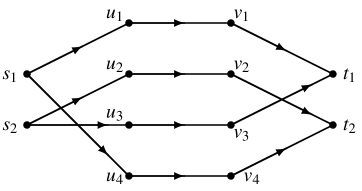
Figure 2: Graph $D=(V,A)$ in Example 11.1

There are (precisely) two integral feasible flows, say, $x_{1}$ and $x_{2}$, each corresponding to a pair of disjoint paths from $\{s_{1},s_{2}\}$ to $\{t_{1},t_{2}\}$, with additional flows on $F$ required by the condition $m(u_{i})=-m(v_{i})$ for $i=1,2,3,4$. Their flow-values on $F$ are given by

$$x_{1}|_{F}=(2,2,3,0)+(1,1,0,0)=(3,3,3,0),\quad x_{2}|_{F}=(2,2,3,0)+(0,0,1,1)=(2,2,4,1),$$

where $x_{1}$ is the unique $F$-dec-min integral flow. Nevertheless, $x_{1}$ has a larger square-sum on $F$ than that of $x_{2}$; the square-sum of $x_{1}|_{F}$ is $27$ and that of $x_{2}|_{F}$ is $25$.

In the fractional (or continuous) case, the feasible flows are precisely the convex combinations of $x_{1}$ and $x_{2}$. That is, $x^{(\lambda)}=\lambda x_{1}+(1-\lambda)x_{2}$ with $0\leq\lambda\leq 1$, and

$$x^{(\lambda)}|_{F}=\lambda(3,3,3,0)+(1-\lambda)(2,2,4,1)=(2+\lambda,2+\lambda,4-\lambda,1-\lambda).$$ (11.4)

This shows that $x_{1}=x^{(1)}$ is the unique $F$-dec-min fractional flow. The square-sum of components of $x^{(\lambda)}|_{F}$ is equal to $4\lambda^{2}-2\lambda+25$, which is minimized at $\lambda=1/4$. We have $x^{(1/4)}|_{F}=(9/4,9/4,15/4,3/4)$, which is decreasingly larger than $x^{(1)}|_{F}=(3,3,3,0)$. Thus, the minimality of square-sum on $F$ does not characterize $F$-dec-minimality even in the fractional case.  

The above example implies, in particular, that an $F$-dec-min fractional flow cannot be obtained by applying the (strongly polynomial) algorithm of Végh [33] for quadratic-cost fractional flows.

Although the above example denies the use of a quadratic cost function for the dec-min flow problem, there remains the possibility of using a more general convex function to formulate the dec-min flow problem. However, the following example indicates that, in the fractional case, the dec-min flow problem cannot be formulated as a minimum-cost flow problem for any choice of a separable convex objective.

Example 11.2.

Let $\varphi$ be an arbitrary strictly convex (smooth) function on ${\bf R}$. Referring to the expression (11.4) of $x^{(\lambda)}|_{F}$, we consider

$$\Phi(\lambda):=\varphi(2+\lambda)+\varphi(2+\lambda)+\varphi(4-\lambda)+\varphi(1-\lambda),$$

which is a separable convex function in the components of $x^{(\lambda)}|_{F}$. Recall that $\lambda=1$ corresponds to $(3,3,3,0)$, which is dec-min among the vectors $x^{(\lambda)}|_{F}$ with $0\leq\lambda\leq 1$. The derivative of $\Phi$ at $\lambda=1$ is positive. Indeed, we have

$$\Phi^{\prime}(\lambda) =2\varphi^{\prime}(2+\lambda)-\varphi^{\prime}(4-\lambda)-\varphi^{\prime}(1-\lambda),\quad\Phi^{\prime}(1)=\varphi^{\prime}(3)-\varphi^{\prime}(0)>0.$$

This implies that the $F$-dec-min flow $x^{(1)}$ is not a minimizer of the separable convex function $\sum_{e\in F}\varphi(x(e))$ over all feasible (fractional) flows $x$. It is emphasized that such discrepancy exists for any choice of $\varphi$.  

The discrepancy of dec-min from convex minimizer demonstrated above implies, in particular, that algorithms for convex cost flows, such as those described in the book of Ahuja, Magnanti, and Orlin [1], cannot be used directly for fractional dec-min flow problem. In this connection, we mention that the fractional dec-min flow problem can be solved in (weakly) polynomial time by solving a sequence of linear programs; see Nace and Orlin [28].

In contrast to the fractional case, the dec-min problem for $Q\subseteq{\bf Z}^{n}$ (in general) can be formulated as a separable convex function minimization, as discussed in [9, Section 3]. In our integral $F$-dec-min flow problem, we can take, for example, a real-valued cost function $\sum_{e\in F}|F|^{x(e)}$ for an integral flow $x$. Here the function $\varphi(k)=|F|^{k}$, defined for all integers $k$, is increasing and strictly convex in the sense that $\varphi(k-1)+\varphi(k+1)>2\varphi(k)$ $(k\in{\bf Z})$. Such convex formulation enables us to solve the dec-min flow problem in (weakly) polynomial time using the approach of Hochbaum and Shanthikumar [19].

References

- [1] Ahuja, R.K., Magnanti, T.L., Orlin, J.B.: Network Flows—Theory, Algorithms and Applications. Prentice-Hall, Englewood Cliffs (1993)
- [2] Borradaile, G., Iglesias, J., Migler, T., Ochoa, A., Wilfong, G., Zhang, L.: Egalitarian graph orientations. Journal of Graph Algorithms and Applications 21, 687–708 (2017)
- [3] Dinits, E.A.: Algorithm for solution of a problem of maximum flow in a network with power estimation (in Russian). Soviet Mathematics Doklady 11, 1277–1280 (1970)
- [4] Edmonds, J., Giles, R.: A min-max relation for submodular functions on graphs. Annals of Discrete Mathematics 1, 185–204 (1977)
- [5] Edmonds, J., Karp, R.M.: Theoretical improvements in algorithmic efficiency for network flow problems. Journal of the ACM 19, 248–264 (1972)
- [6] Ford, L. R., Jr., Fulkerson, D.R.: Flows in Networks. Princeton University Press, Princeton (1962)
- [7] Frank, A.: Kernel systems of directed graphs. Acta Scientiarum Mathematicarum 41, 63–76 (1979)
- [8] Frank, A.: Connections in Combinatorial Optimization. Oxford University Press, Oxford (2011)
- [9] Frank, A., Murota, K.: Discrete decreasing minimization, Part II: Views from discrete convex analysis, arXiv: 1808.08477, August 2018.
- [10] Frank, A., Murota, K.: Decreasing minimization on M-convex sets: Background and structures. Mathematical Programming, published online (October 27, 2021) https://doi.org/10.1007/s10107-021-01722-2
- [11] Frank, A., Murota, K.: Decreasing minimization on M-convex sets: Algorithms and applications. Mathematical Programming, published online (October 15, 2021) https://doi.org/10.1007/s10107-021-01711-5
- [12] Frank, A., Murota, K.: Fair integral submodular flows. Submitted for publication, arXiv: http://arxiv.org/abs/2012.07325 (December, 2020)
- [13] Fujishige, S.: Lexicographically optimal base of a polymatroid with respect to a weight vector. Mathematics of Operations Research 5, 186–196 (1980)
- [14] Fujishige, S.: Submodular Functions and Optimization, 2nd edn. Annals of Discrete Mathematics 58, Elsevier, Amsterdam (2005)
- [15] Georgiadis, L., Georgatsos, P., Floros, K., Sartzetakis, S.: Lexicographically optimal balanced networks. IEEE/ACM Transactions on Networking 10, 818–829 (2002)
- [16] Goemans, M.X., Gupta, S., Jaillet, P.: Discrete Newton’s algorithm for parametric submodular function minimization. In: Eisenbrand, F., Koenemann, J. (eds.) Integer Programming and Combinatorial Optimization. Lecture Notes in Computer Science, vol. 10328, pp. 212–227 (2017)
- [17] Goldberg, A.V., Tarjan, R.E.: A new approach to the maximum-flow problem. Journal of the ACM 35, 921–940 (1988)
- [18] Harvey, N.J.A., Ladner, R.E., Lovász, L., Tamir, T.: Semi-matchings for bipartite graphs and load balancing. Journal of Algorithms 59, 53–78 (2006)
- [19] Hochbaum, D.S., Shanthikumar, J.G.: Convex separable optimization is not much harder than linear optimization. Journal of the Association for Computing Machinery 37, 843–862 (1990)
- [20] Hoffman, A.J.: Some recent applications of the theory of linear inequalities to extremal combinatorial analysis. In: Bellman, R., Hall, M., Jr. (eds.) Combinatorial Analysis (Proceedings of the Symposia of Applied Mathematics 10) pp. 113–127. American Mathematical Society, Providence, Rhode Island (1960)
- [21] Ibaraki, T., Katoh, N.: Resource Allocation Problems: Algorithmic Approaches. MIT Press, Cambridge, MA (1988)
- [22] Kaibel, V., Onn, S., Sarrabezolles, P.: The unimodular intersection problem. Operations Research Letters 43, 592–594 (2015)
- [23] Katoh, N., Shioura, A., Ibaraki, T.: Resource allocation problems. In: Pardalos, P.M., Du, D.-Z., Graham, R.L. (eds.) Handbook of Combinatorial Optimization, 2nd ed., Vol. 5, pp. 2897-2988, Springer, Berlin (2013)
- [24] Megiddo, N.: Optimal flows in networks with multiple sources and sinks. Mathematical Programming 7, 97–107 (1974)
- [25] Megiddo, N.: A good algorithm for lexicographically optimal flows in multi-terminal networks. Bulletin of the American Mathematical Society 83, 407–409 (1977)
- [26] Moulin, H.: Fair Division and Collective Welfare. MIT Press, Cambridge, MA (2003)
- [27] Murota, K.: Discrete Convex Analysis. Society for Industrial and Applied Mathematics, Philadelphia (2003)
- [28] Nace, D., Orlin, J.B.: Lexicographically minimum and maximum load linear programming problems. Operations Research 55, 182–187 (2007)
- [29] Plaut, B., Roughgarden, T.: Almost envy-freeness with general valuations. SIAM Journal on Discrete Mathematics 34, 1039–1068 (2020)
- [30] Radzik, T.: Fractional combinatorial optimization. In: Pardalos, P.M., Du, D.-Z., Graham, R.L. (eds.) Handbook of Combinatorial Optimization, 2nd edn., pp. 1311–1355. Springer Science+Business Media, New York (2013)
- [31] Schrijver, A.: Combinatorial Optimization—Polyhedra and Efficiency. Springer, Heidelberg (2003)
- [32] Tardos, É.: A strongly polynomial minimum cost circulation algorithm. Combinatorica 5, 247–255 (1985)
- [33] Végh, L.A.: A strongly polynomial algorithm for a class of minimum-cost flow problems with separable convex objectives. SIAM Journal on Computing 45, 1729–1761 (2016)