FINAL MASSES OF GIANT PLANETS III: EFFECT OF PHOTOEVAPORATION AND A NEW PLANETARY MIGRATION MODEL

Abstract

We herein develop a new simple model for giant planet formation, which predicts the final mass of a giant planet born in a given disk, by adding the disk mass loss due to photoevaporation and a new type II migration formula to our previous model. The proposed model provides some interesting results. First, it gives universal evolution tracks in the diagram of planetary mass and orbital radius, which clarifies how giant planets migrate at growth in the runaway gas accretion stage. Giant planets with a few Jupiter masses or less suffer only a slight radial migration in the runaway gas accretion stage. Second, the final mass of giant planets is approximately given as a function of only three parameters: the initial disk mass at the starting time of runaway gas accretion onto the planet, the mass loss rate due to photoevaporation, and the starting time. On the other hand, the final planet mass is almost independent of the disk radius, viscosity, and planetary orbital radius. The obtained final planet mass is $\lesssim$10% of the initial disk mass. Third, the proposed model successfully explains properties in the mass distribution of giant exoplanets with the mass distribution of observed protoplanetary disks for a reasonable range of the mass loss rate due to photoevaporation.



1 INTRODUCTION

One of the main goals of the planet formation theory is to explain the statistics of thousands of exoplanets using the statistical properties of observed protoplanetary disks (e.g., Andrews et al. 2010) in a consistent manner. In the present paper, we try to explain the masses of giant exoplanets.

In the core accretion model, giant planets are formed with the following two growth stages in a protoplanetary disk (e.g., Mizuno 1980). The first stage is the formation of the planetary solid core via accumulation of planetesimals and pebbles (e.g., Kokubo & Ida 2002; Lambrechts & Johansen 2014). Once the solid core grow to the critical mass ($\sim$10$M_{\oplus}$) for gravitational collapse of its envelope, a rapid runaway accretion of the disk gas onto the planet proceeds after a relatively slow contraction of the envelope (e.g., Pollack et al. 1996; Ikoma et al. 2000; Hubickyj et al. 2005), which is the second stage. In the present paper, we focus on the latter runaway gas accretion stage of the giant planet formation since the final masses of the gaseous giant planets is governed by the runaway gas accretion. Although a fast type-I planetary migration at the stage of the solid core growth is also one of serious problems in giant planet formation (e.g., Tanaka et al. 2002; Paardekooper et al. 2011), this first stage is out of scope of the present study.

The formation of giant planets is governed by the gas accretion rate onto the planets and the radial migration speed. A massive planet with $\gtrsim$ several tens of earth masses opens a low-density gap around its orbit in the protoplanetary disk with the planetary torque (e.g., Lin & Papaloizou 1986; Crida et al. 2006). The disk gap considerably changes the planetary growth and migration, as originally proposed by Lin & Papaloizou (1986). Their original gap model assumes that almost no gas exists inside the gap and that no mass flow across the gap exists. Then the gap opening terminates growth of the planet. Because of no gap-crossing flow, the planet is locked in the gap and migrates with the disk viscous evolution, which is the mechanism of the original type II migration. Many studies on planet formation have adopted the type II planetary migration and termination of growth due to the gap.

However, two- and three-dimensional hydro-dynamical simulations showed that disk gas can easily cross the gap and also accrete onto the planet even for the gap created by a Jupiter-mass planet or larger (e.g., Kley 1999; Lubow et al. 1999; Masset & Snellgrove 2001; D’Angelo et al. 2003; Machida et al. 2010; Zhu et al. 2011). Thus the planetary growth continues even after the gap opening though the low-density gap reduces the mass accretion rate. The surface density inside the gap was examined by recent hydro-dynamical simulations and an empirical model of the gap surface density is proposed (e.g., Duffell & MacFadyen 2013; Fung et al. 2014; Kanagawa et al. 2015a, 2016, 2017). Tanigawa & Tanaka (2016, hereinafter Paper 2) constructed an analytic formula for the mass accretion rate onto the planet, by using the empirical model for the gap surface density. This formula reproduces very well the results of hydro-dynamical simulations by D’Angelo et al. (2003) and Machida et al. (2010). The present paper also uses this formula.

The type II migration of giant planets has been problematic in previous studies on giant planet formation (e.g., Ida & Lin 2004; Mordasini et al. 2009; Hasegawa & Ida 2013; Ida et al. 2018; Bitsch et al. 2015, 2019). Duffell et al. (2014) found a further faster type II migration in their hydro-dynamical simulations. Their obtained migration speeds are higher than those of the planet-dominated type II migration based on the original model (e.g., Armitage 2007) by a factor of 3. Their type II migration speeds were confirmed by Dürmann & Kley (2015, 2017) and Robert et al. (2018). In Paper 2, however, we found that the reduction in the disk surface density due to gas accretion onto the planet slows down the type II migration sufficiently. Moreover, Kanagawa et al. (2018) recently proposed a new model for type II migration. In their new model, the planet mainly interact with the disk gas inside the gap and the planetary migration speed is proportional to the reduced surface density in the gap. A similar idea on the type II migration had been first pointed out by D’Angelo and Lubow(2008). The new model proposed by Kanagawa et al. reproduces very well the results obtained from the previous hydro-dynamical simulations of type II migration (Duffell et al. 2014; Dürmann & Kley 2015) and from the simulations by Kanagawa et al. The present paper uses their new formula for type II migration to revise our model.

In Paper 2, we also suggested that the final mass of a giant planet should be much more massive in the MMSN disk than the Jupiter mass. However, we did not take into account the disk mass loss due to the photoevaporation directly. Such a dissipation effect of photoevaporation is required in order to explain the disk lifetime and the rareness of the transitional disks (e.g., Clarke et al. 2001; Alexander et al. 2014). The present paper considers the disk mass loss due to photoevaporation, which would reduce the final planet mass for a given disk.

Previous studies on the population synthesis of giant planets have already examined the origin of statistics of exoplanets in detail (e.g., Benz et al. 2004 and papers therein; Ida et al. 2018). In order to examine the distributions of the final masses and orbital radii of planets, they performed Monte Carlo simulations with probability distribution functions of various disk parameters. However, it is not clear yet what mass and orbital radius a planet will finally have in a given disk, because of uncertainties in disk models, the viscosity parameter, and models of planetary growth and migration. Moreover, the dependence of the final planet mass on the disk parameters (e.g., disk mass, radius, viscosity, and mass loss rate due to photoevaporation) is unclear. In addition, accurate empirical formulas for planetary growth rate and migration speed mentioned above were not used properly in their population synthesis calculations.

In the present paper, we revise our simple model for giant planet formation by including a new type II migration formula and the disk mass loss due to photoevaporation by EUV. We show that our new model can clearly predict the final mass of giant planets for a given disk, despite of many unfixed parameters in current disk models.

In Section 2, we briefly describe formulas of accretion rate and migration speed that have already been tested through hydro-dynamical simulations. These formulas directly give universal evolution tracks in the diagram of planetary mass and orbital radius for the runaway gas accretion stage, although the prediction of the final planet mass also requires the disk model. In Section 3, we present a very simple disk model that includes the disk mass loss due to photoevaporation by EUV. Using this simple disk model, we derive a direct expression for the planetary growth rate. In Section 4, we examine the time evolution and the final mass of giant planets for a reasonable parameter range. Our results for the final planet mass will also be applied to the origin of exoplanets. In Section 5, we summarize our results.

2 Models of growth and migration for giant planets

2.1 Assumptions

For giant planet formation, we adopt the core-accretion model. We focus on the stage in which the solid core of a planet is more massive than the critical core mass (Mizuno 1980, Ikoma et al. 2000). Then, the planet grows primarily via runaway accretion of the disk gas. In the proposed model, as an initial condition, we assume that such a massive solid core exists in the disk. For simplicity, we examine the growth and migration of a single giant planet in the gaseous disk and neglect the effect of other planets.

2.2 Growth Rate and Migration Rate of a Planet

We adopt the rate of gas accretion onto a planet modeled by Paper 2. The growth rate of the planet via the runaway gas accretion (or the accretion rate to the planet), $dM_{p}/dt$, is given by

$$\frac{dM_{p}}{dt}=D\,\Sigma_{\mbox{\scriptsize{gap}}}.$$ (1)

The coefficient $D$ is empirically obtained as (Tanigawa & Watanabe 2002)

$$D=0.29\left(\frac{M_{p}}{M_{*}}\right)^{4/3}\left(\frac{h_{p}}{r_{p}}\right)^{-2}r_{p}^{2}\Omega_{p},$$ (2)

where $M_{*}$ and $r_{p}$ are the mass of the central star and the orbital radius of the planet, respectively. The subscript $p$ of the scale height $h$ and the Keplerian angular velocity $\Omega$ indicates values at $r=r_{p}$. The surface density in the planetary gap, $\Sigma_{\mbox{\scriptsize{gap}}}$, is also given by an empirical formula (e.g., Duffell & MacFadyen 2013; Kanagawa et al. 2015a, 2015b)

$$\Sigma_{\mbox{\scriptsize{gap}}}=\frac{\Sigma_{\mbox{\scriptsize{out}}}}{1+0.04K},$$ (3)

where the non-dimensional parameter $K$ is given by

$$K=\left(\frac{M_{p}}{M_{*}}\right)^{2}\left(\frac{h_{p}}{r_{p}}\right)^{-5}\alpha^{-1}.$$ (4)

Moreover, $\Sigma_{\mbox{\scriptsize{out}}}$ is the surface density just outside of the gap, and $\alpha$ is the viscosity parameter of the disk (Shakura & Sunyaev 1973). Note that Equation (3) derived from hydro-dynamical simulations gives a much shallower gap than the previous one-dimensional analytic models (e.g., Lubow & D’Angelo 2006; Tanigawa & Ikoma (Paper 1)). Owing to the shallow gap, the gas accretion onto the giant planet does not terminate even after the gap is formed. The mass accretion rate of Equation (1) reproduces very well the results of hydro-dynamical simulations by D’Angelo et al. (2003) and Machida et al. (2010) for planets heavier than 10$M_{\oplus}$, as shown in Figure 1 of Paper 2.

Exactly speaking, the gap surface density of Equation (3) represents the surface density around $r=r_{p}\pm 2R_{\mbox{\scriptsize{Hill}}}$ rather than the lowest value at $r_{p}$ for a deep gap, where $R_{\mbox{\scriptsize{Hill}}}$ is the Hill radius of the planet (e.g., Fung et al. 2014; Kanagawa et al. 2017). It would be reasonable that Equation (3) is used for the estimates of the accretion rate and the type II migration speed since those rates are determined by the surface densities around $r=r_{p}\pm 2R_{\mbox{\scriptsize{Hill}}}$ rather than that at $r_{p}$ (Tanigawa & Watanabe 2002; D’Angelo & Lubow 2008).

It should be also noted that a slow Kelvin-Helmholtz contraction of the planetary envelope occurs between the stages of the solid core growth and the runaway gas accretion (e.g., Pollack et al. 1996; Ikoma et al. 2000). The slow contraction of the envelope regulates the mass accretion rate for planets with $M_{p}\sim M_{\mbox{\scriptsize{crit}}}$. In this slow contraction stage, Equation (1) overestimates the mass accretion rate. The timing of the transition from the slow contraction stage to the runaway accretion stage where the accretion rate of Equation (1) is valid can be estimated as follows. We can estimate the Kelvin-Helmholtz contraction time for the envelope of a planet with the mass $M_{p}$ as

$$\tau_{\mbox{\scriptsize{KH}}}\simeq 1\times 10^{3}\left(\frac{M_{p}}{30M_{\oplus}}\right)^{-2.5}\left(\frac{\kappa}{0.05\mbox{cm}^{2}\mbox{g}^{-1}}\right)\mbox{yr},$$ (5)

by replacing the core mass $M_{\mbox{\scriptsize{core}}}$ with $M_{p}$ in the analytic contraction time derived by Ikoma et al. (2000). In Equation (5), $\kappa$ is the opacity of the planetary envelope. The opacity of $\kappa$ =0.05 g cm^-2 is consistent with Movshovitz & Podolak (2008) who calculated the envelop opacity, taking into account dust growth and sedimentation in the envelope. A contraction time similar to Equation (5) is adopted in the planetary population synthesis calculations (e.g., Ida & Lin 2004, Benz et al. 2014, Ida et al. 2018). Equation (5) can also explain the mass accretion rates obtained by Lambrechts et al. (2019) with their three-dimensional non-isothermal hydro-dynamical simulations for $M_{p}<100M_{\oplus}$, by using the value of the opacity they adopted. The mass accretion rate regulated by the slow contraction is given by $M_{p}/\tau_{\mbox{\scriptsize{KH}}}$. By equating this accretion rate with Equation (1), we can estimate the planet mass at the transition from the slow contraction to the runaway accretion as $30(\kappa/0.05\mbox{cm}^{2}\mbox{g}^{-1})^{6/13}M_{\oplus}$ for $\Sigma_{\mbox{\scriptsize{gas}}}=\mbox{100g}\,\mbox{cm}^{2}$ and the disk aspect ratio of $h/r=0.05$ at 5AU. Hence, for planets with $M_{p}>30M_{\oplus}$, the envelope contraction is rapid enough and Equation (1) is valid.

The radial migration speed of the planet is generally expressed with the torque on a planet, $\Gamma$, as

$$\frac{d}{dt}\ln r_{p}=2\frac{d}{dt}\ln L_{p}=\frac{2\Gamma}{M_{p}r_{p}^{2}\Omega_{p}},$$ (6)

where $L_{p}$ is the angular momentum of the planet. Kanagawa et al. (2018) found that by using the gap surface density $\Sigma_{\mbox{\scriptsize{gap}}}$, the torque on a planet embedded in the disk gap (i.e., the torque of type II planetary migration) is given by an expression similar to that for the type I torque (e.g., Tanaka et al. 2002):

$$\Gamma=-3.0\left(\frac{M_{p}}{M_{*}}\right)^{2}\left(\frac{h_{p}}{r_{p}}\right)^{-2}r_{p}^{4}\Omega_{p}^{2}\Sigma_{\mbox{\scriptsize{gap}}}.$$ (7)

From Equations (6) and (7), the migration speed of a planet is given by

$$\frac{d}{dt}\ln r_{p}=-6.0\,\frac{M_{p}}{M_{*}}\left(\frac{h_{p}}{r_{p}}\right)^{-2}\frac{r_{p}^{2}\,\Sigma_{\mbox{\scriptsize{gap}}}}{M_{*}}\Omega_{p}.$$ (8)

The migration speed for type II migration also reproduces very well the results obtained from the previous hydro-dynamical simulations of type II migration (Dürmann & Kley 2014, Duffell et al. 2014) and from the simulations by Kanagawa et al. Type II migration was previously thought to be caused by the interaction with gap edges (i.e., outside of the gap) (e.g., Lin & Papaloizou 1986, 1993; Armitage 2007). On the other hand, the new more accurate formula by Kanagawa et al. indicates that the planet mainly interacts with the gas inside the gap. For a less massive planet forming no gap, Kanagawa et al’s formula is reduced to that of type I migration. In the present paper, we use this new formula for the type II planetary migration speed, although Paper 2 basically adopted the previous type II migration model.

The present paper does not include type III migration or dynamical corotation torque which appear only in very massive disks (e.g., Masset & Papaloizou 2003; Paardekooper 2014; Pierens & Raymond 2016). Pierens & Raymond (2016) showed with their hydro-dynamical simulations that planets experience a more rapid (outward) migration than type II due to the dynamical corotation torque during their growth. In their simulations, however, planets grow to about 10 jupiter masses within $1\times 10^{4}$ yrs. Thus it is expected that those bodies might grow to several tens of jupiter masses (i.e., the mass range of brown dwarfs or red dwarfs) within the typical disk lifetime of $\sim 10^{6}$ yrs. Formation of such massive bodies are beyond the scope of the present study.

2.3 Universal Evolution Tracks in the Mass-Orbit Diagram

In our model, the growth rate and the migration speed are both proportional to $\Sigma_{\mbox{\scriptsize{gap}}}$. The time evolution of the planet mass and orbital radius depends on $\Sigma_{\mbox{\scriptsize{gap}}}(t)$ or the disk model described in the next section. Here, we consider planetary evolution tracks in the diagram of mass and orbital radius. Interestingly, the evolution tracks are independent of the model of the protoplanetary disk, as shown below.

Dividing Equation (1) by (8) and using (2), we obtain a simple differential equation for the evolution tracks:

$$\frac{d\ln M_{p}}{d\ln r_{p}}=\frac{0.29}{6.0}\left(\frac{M_{p}}{M_{*}}\right)^{-2/3}=\left(\frac{M_{p}}{M_{\mbox{\scriptsize{th}}}}\right)^{-2/3},$$ (9)

where the threshold mass $M_{\mbox{\scriptsize{th}}}$ is given by

$$M_{\mbox{\scriptsize{th}}}=\left(\frac{0.29}{6.0}\right)^{3/2}M_{*}=0.011M_{*}.$$ (10)

This simple form of Equation (9) is available because $dM_{p}/dt$ and $d\ln r_{p}/dt$ are both proportional to $(h_{p}/r_{p})^{-2}\Sigma_{\mbox{\scriptsize{gap}}}$. Solving Equation (9), we obtain an analytic expression for the universal evolution tracks in the diagram of planetary mass and orbital radius as

$$\frac{r_{p}}{r_{0}}=\exp\left\{-\frac{3}{2}\left[\left(\frac{M_{p}}{M_{\mbox{\scriptsize{th}}}}\right)^{2/3}-\left(\frac{M_{0}}{M_{\mbox{\scriptsize{th}}}}\right)^{2/3}\right]\right\},$$ (11)

where $M_{0}$ and $r_{0}$ are the initial mass and initial orbital radius of the planet, respectively. We recall that the obtained evolution tracks are completely independent of the disk model. Our evolution tracks are independent of the disk gap model of Equation (3), too.

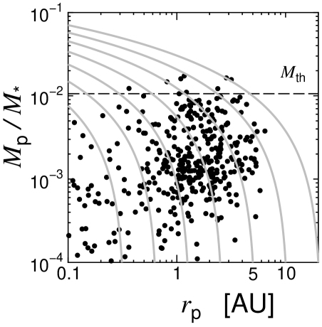
Figure 1: Universal evolution tracks of giant planets in the mass-orbit diagram in the runaway gas accretion stage. Our evolution tracks are completely independent of the disk model whereas the disk model affects termination of planetary growth on each track. The initial mass, $M_{0}$, is set to be $10^{-4}M_{*}$ and the initial orbital radii, $r_{0}$, are varied from 0.31AU to 20AU. Data of exoplanets observed by the radial-velocity method (http://exoplanets.org) are also plotted. As for masses of exoplanets, the observed values of $M_{p}\sin i$ are simply used.

Figure 1 shows the universal evolution tracks of Equation (11) in the diagram of planet mass and orbital radius. In Figure 1, we also plot the data of exoplanets observed by the radial-velocity method, which have a weak observational bias compared with the radial distribution of the exoplanets discovered by transit surveys. Planets less massive than the threshold mass $M_{\mbox{\scriptsize{th}}}$ ($\simeq\!\!10M_{J}$ for a solar-mass star) do not suffer much radial migration. This is because the migration timescale is longer than the growth time for $M_{p}<M_{\mbox{\scriptsize{th}}}$. The final orbital radius of a planet with $M_{\mbox{\scriptsize{th}}}$ is approximately 1/5 of the initial orbital radius. Previous studies reported a problematic rapid type II migration in the giant planet formation, as described in Introduction. However, our model shows that very massive exoplanets exceeding $M_{\mbox{\scriptsize{th}}}$ plotted in Figure 1 can also be formed from solid cores initially located within 20 AU. Our model succeeds in fixing the problem of type II migration in giant planet formation.

Slight migrations for Jupiter-mass planets or less, on the other hand, make the origin of hot Jupiters difficult to explain. Orbital radii of planets can be shifted by mutual interactions between multiple planets, which are not included in our model. As an explanation of hot Jupiters, the model that considers the planet-planet scattering followed by the tidal circularization (e.g., Rasio & Ford 1996; Nagasawa et al. 2008; Winn et al. 2010) is more plausible than the model that considers type II migration. The type I migration of solid planetary cores before the runaway gas accretion stage can be an alternative possible origin of hot Jupiters. Solid planetary cores can easily migrate inward since their growth time is expected to be much longer than that at the runaway gas accretion stage.

A relatively large number of giant exoplanets are observed in the radial range of from 1 to 3 AU in Figure 1. These crowded exoplanets can be explained if a large number of massive solid cores are formed from 1.5 AU to 4 AU of protoplanetary disks. Such massive planetary embryos may be naturally formed just outside of the snow line, which is located at 1 to 3 AU.

Note that the disk model affects where and how the planetary growth terminates on an evolution track (i.e., the final mass and location of the planet). We will discuss these items, using a simple disk model described in the next section.

It should be also noticed that the torque and the migration speed in Kanagawa et al’s formulas (Equations (7) and (8)) can be underestimated in the absolute values in the regime of type I migration (i.e., for $M_{p}\lesssim 10^{-4}M_{*}$). Although the coefficient of the torque is fixed as $-3.0$ in Equation (7), the torque depends on the radial gradients of the disk surface density and temperature in the accurate type I formulas (e.g., Tanaka et al. 2002; Paardekooper et al. 2011). Owing to steep radial distributions in $\Sigma$ and/or $T$, the accurate type I migration can be faster than Equation (8) by the factor of 2 or 3. However, such a possible enhancement in the migration speed would hardly change the result of a slight migration for $M_{p}\sim 10^{-4}M_{*}$ because the migration timescale given by Equation (8) is about 20 times as long as the growth time at $M_{p}\sim 10^{-4}M_{*}$.

3 Disk model

3.1 Self-similar Solution of Accretion Disks

Our simple disk model is based on the self-similar solution of accretion disks with the viscosity $\nu$ being proportional to $r^{\gamma}$ (Lynden-Bell & Pringle 1974; Hartmann et al. 1998). The temperature distribution can be more complex than a single power-law in realistic disk models. Such a complex disk model should be examined in the future work. In this simple model, we also include the effects of photoevaporation of disk gas by EUV radiation from the central star and gas accretion onto a planet. We assume that the orbital radius of the planet $r_{p}$ and the radial location $r_{g}$, where the photoevaporation primarily occurs, are much smaller than the disk radius. Then, the planet and the photoevaporation would have only minor effects on the evolution of the outer part of the disk, which contains most of the (total) disk mass. Gorti & Hollenbach (2009) suggested that FUV radiation from the central star can cause rapid erosion of the outer disk. Such strong photoevaporation by FUV can reduce the disk mass in a relatively short time ($\sim 10^{6}$yr). However, since the mass loss rate by FUV photoevaporation is still uncertain to about an order of magnitude (e.g., Alexander et al. 2014), we do not include photoevaporation by FUV in our disk model.

At an outer part of the disk, the surface density is then simply given by the self-similar solution:

$$\Sigma(r,t)=\frac{M_{d}(t)}{6\pi(2-\gamma)\nu t}\exp\left[-\left(\frac{r}{R_{d}(t)}\right)^{2-\gamma}\right].$$ (12)

where $\nu=\nu_{0}r^{\gamma}$ and the characteristic disk radius $R_{d}$ is given by

$$R_{d}=[\,3(2-\gamma)^{2}\nu_{0}\,t\,]^{\frac{1}{2-\gamma}}.$$ (13)

The disk mass $M_{d}$ decreased as follows:

$$M_{d}(t)=M_{d}(t_{0})\left(\frac{t}{t_{0}}\right)^{-\frac{1}{4-2\gamma}}.$$ (14)

At the intermediate disk region in which $r_{p},r_{g}\ll r\ll R_{d}$, the surface density and the disk accretion rate $\dot{M}_{d}$ are approximately given by

$$\Sigma=\frac{M_{d}(t)}{3\pi(4-2\gamma)\nu t},\qquad\!\!\dot{M}_{d}=\frac{M_{d}(t)}{(4-2\gamma)t}\!\!\qquad(\mbox{for }\>\>r\ll R_{d})$$ (15)

and we obtain the well-known relation between them as

$$\Sigma=\frac{\dot{M}_{d}}{3\pi\nu}\qquad\qquad(\mbox{for }\>\>r\ll R_{d}).$$ (16)

Note that the time-evolution of the disk mass and the accretion rate are independent of the disk viscosity in Equations (14) and (15). Then, the disk surface density is inversely proportional to the viscosity.

We assume the disk temperature as $280(r/1\mbox{AU})^{-1/2}$K (Hayashi et al. 1985). Then, the disk aspect ratio (i.e., the ratio of the scale height to the radius) is given by

$$\frac{h}{r}=0.05\left(\frac{r}{5\mbox{AU}}\right)^{1/4}.$$ (17)

Using the parameter $\alpha$, the disk viscosity is also expressed as

$$\nu=\alpha h^{2}\Omega.$$ (18)

In the next section, we adopt $\gamma=1$ in the nominal case, assuming a constant $\alpha$.

3.2 Effect of Photoevaporation

In our model, we regard the mass loss rate due to the photoevaporation $\dot{M}_{\mbox{\scriptsize{w}}}$ as a parameter. We assume that the mass loss due to photoevaporation occurs primarily outside the planet orbit. Even for the case in which the photoevaporation inside the planet orbit is not negligible, the following treatment for photoevaporation would also be valid by considering $\dot{M}_{\mbox{\scriptsize{w}}}$ as the mass loss rate only outside of the planet orbit.

If no mass loss due to photoevaporation exists, then the mass supply rate to the planet-forming inner region, $\dot{M}_{\mbox{\scriptsize{sup}}}$, is equal to the disk accretion rate, $\dot{M}_{d}$. When the photoevaporation is effective, the mass supply rate to the planet-forming region is given by

$$\dot{M}_{\mbox{\scriptsize{sup}}}=\dot{M}_{d}-\dot{M}_{\mbox{\scriptsize{w}}}$$ (19)

if $\dot{M}_{d}\geq\dot{M}_{\mbox{\scriptsize{w}}}$. Then, the disk surface density in the planet-forming inner region is given by

$$\Sigma=\frac{\dot{M}_{\mbox{\scriptsize{sup}}}}{3\pi\nu}=\frac{\dot{M}_{d}-\dot{M}_{\mbox{\scriptsize{w}}}}{3\pi\nu}.$$ (20)

The disk accretion rate decreases gradually. The time at which planet growth stops, $t_{\mbox{\scriptsize{end}}}$, is determined by the equation $\dot{M}_{\mbox{\scriptsize{sup}}}=0$, i.e.,

$$\dot{M}_{d}(t_{\mbox{\scriptsize{end}}})=\dot{M}_{\mbox{\scriptsize{w}}}.$$ (21)

Using Equation (15), we can rewrite Equation (21) as

$$\left(\frac{t_{\mbox{\scriptsize{end}}}}{t_{0}}\right)^{\frac{5-2\gamma}{4-2\gamma}}=\frac{{M}_{d}(t_{0})}{(4-2\gamma)t_{0}\dot{M}_{\mbox{\scriptsize{w}}}}.$$ (22)

We regard $t_{0}$ as the starting time of the runaway gas accretion onto the planet, and $M_{d}(t_{0})$ is the disk mass at the starting time. When $M_{d}(t_{0})<(4-2\gamma)t_{0}\dot{M}_{\mbox{\scriptsize{w}}}$, Equation (22) gives $t_{\mbox{\scriptsize{end}}}<t_{0}$. This means that runaway gas accretion onto the planet cannot occur because of gas dissipation at the planet-forming region before $t_{0}$ due to strong photoevaporation. By integrating Equation (19) from $t_{0}$ to $t_{\mbox{\scriptsize{end}}}$, we can also obtain the total gaseous mass supplied to the planet-forming region from $t_{0}$ up to $t_{\mbox{\scriptsize{end}}}$, $M_{\mbox{\scriptsize{sup}}}$, as

$$M_{\mbox{\scriptsize{sup}}} = \int^{t_{\mbox{\scriptsize{end}}}}_{t_{0}}\dot{M}_{\mbox{\scriptsize{sup}}}\,dt$$

$$= {M}_{d}(t_{0})\left[1-\left(\frac{t_{\mbox{\scriptsize{end}}}}{t_{0}}\right)^{-\frac{1}{4-2\gamma}}\right]-\dot{M}_{\mbox{\scriptsize{w}}}(t_{\mbox{\scriptsize{end}}}-t_{0})$$

$$= {M}_{d}(t_{0})\left[1-\frac{5-2\gamma}{4-2\gamma}\left(\frac{t_{\mbox{\scriptsize{end}}}}{t_{0}}\right)^{-\frac{1}{4-2\gamma}}\right]+\,t_{0}\dot{M}_{\mbox{\scriptsize{w}}}.$$

3.3 Effects of Gas Accretion onto the Planet

Lubow & D’Angelo (2006) gave the analytic expression of the surface density reduced by the gas accretion onto a planet as:

$$\Sigma_{\mbox{\scriptsize{out}}}(r_{p})=\frac{\dot{M}_{d}-\dot{M}_{p}}{3\pi\nu(r_{p})}.$$ (24)

In the above, we used the notation, $\Sigma_{\mbox{\scriptsize{out}}}$, which is the surface density just outside the planetary gap. This is because the effect of the planetary gap is not included in Equation (24). This expression is not valid when the photoevaporation is effective. However, we can readily include the effect of photoevaporation in Equation (24), by simply replacing $\dot{M}_{d}$ with $\dot{M}_{\mbox{\scriptsize{sup}}}$:

$$\Sigma_{\mbox{\scriptsize{out}}}(r_{p})=\frac{\dot{M}_{d}-\dot{M}_{\mbox{\scriptsize{w}}}-\dot{M}_{p}}{3\pi\nu(r_{p})}.$$ (25)

This is the expression of $\Sigma_{\mbox{\scriptsize{out}}}$ including both the effects of photoevaporation and gas accretion onto the planet. The mass flux crossing the gap to the innermost disk is given by $\dot{M}_{d}-\dot{M}_{\mbox{\scriptsize{w}}}-\dot{M}_{p}$ and it is reduced by the gas accretion onto the planet and the photoevaporation. In Figure 2, we summarize our simple disk model.

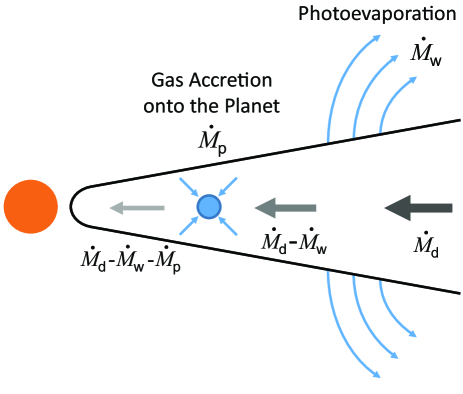
Figure 2: Schematic diagram of the proposed simple disk model. Because of photoevaporation with mass loss rate $\dot{M}_{\mbox{\scriptsize{w}}}$, the mass supply rate to the planet-forming region is reduced to $\dot{M}_{d}-\dot{M}_{\mbox{\scriptsize{w}}}$. The disk accretion rate at the innermost disk is further reduced to $\dot{M}_{d}-\dot{M}_{\mbox{\scriptsize{w}}}-\dot{M}_{p}$ due to gas accretion onto the planet. From these disk accretion rates, the surface density distribution of this viscous accretion disk is obtained in the proposed disk model.

3.4 Direct Expression for the Planetary Growth Rate

The growth rate, $\dot{M}_{p}$, included in Equation (25) depends on $\Sigma_{\mbox{\scriptsize{gap}}}$ (or $\Sigma_{\mbox{\scriptsize{out}}}$), as shown in Equation (1). By solving the coupled equations (1), (3), and (25), we obtain

$$\Sigma_{\mbox{\scriptsize{gap}}}=\frac{1}{1+0.04K}\left(1+\frac{D^{\prime}}{3\pi\nu(r_{p})}\right)^{-1}\frac{\dot{M}_{d}-\dot{M}_{\mbox{\scriptsize{w}}}}{3\pi\nu(r_{p})}$$ (26)

and

$$\dot{M}_{p}=\frac{D^{\prime}/3\pi\nu(r_{p})}{1+D^{\prime}/3\pi\nu(r_{p})}\,(\dot{M}_{d}-\dot{M}_{\mbox{\scriptsize{w}}}),$$ (27)

where $D^{\prime}$ is given by

$$D^{\prime}=\frac{D}{1+0.04K}$$ (28)

and $D$ and $K$ both depend on $M_{p}$ and $r_{p}$, as shown in Equations (2) and (4). The first and second factors in the RHS of Equation (26) represent the reduction factors of the surface density due to the planetary gap and due to the gas accretion onto the planet, respectively. Both factors reduces the type II migration speed as well as the gas accretion rate onto the planet since these rates are proportional to $\Sigma_{\mbox{\scriptsize{gap}}}$. Equation (27) gives a direct expression for the planetary growth rate. Note that the disk accretion rate $\dot{M}_{d}$ is given by Equation (15) and that the orbital radius $r_{p}$ is dependent on $M_{p}$, as show in Equation (11).

When the ratio $D^{\prime}/(3\pi\nu)$ is large, the mass accretion rate $\dot{M}_{p}$ is nearly equal to the supply rate $\dot{M}_{d}-\dot{M}_{\mbox{\scriptsize{w}}}$. This means that an insufficient mass supply rate (or a low disk accretion rate) regulates $\dot{M}_{p}$. The regulation of $\dot{M}_{p}$ due to a small disk accretion rate is taken into account in many population synthesis calculations. The regulation of $\dot{M}_{p}$ are originated from the surface density reduction due to the second factor in Equation (26). This surface density reduction due to a low disk accretion rate also slow down the type II migration, as first pointed out by Tanigawa & Tanaka (2016). Robert et al. (2018) also found the slow-down of type II migration due to a rapid gas accretion on the planet in their hydro-dynamical simulations. However, recent population synthesis calculations does not include the slowing mechanism yet, even though they include the regulation of $\dot{M}_{p}$ due to a low disk accretion rate (e.g., Ida et al. 2018, Johansen et al. 2019, Bitsch et al. 2019). Such an inconsistent treatment in the growth rate and the migration speed breaks down the universality of the evolution tracks proposed in Section 2.3.

Estimating the non-dimensional ratio $D^{\prime}/(3\pi\nu)$ is valuable. We consider a deep-gap case in which $0.04K\gg 1$. From Equation (4), this corresponds to the case of relatively massive planets having masses that satisfy

$$M_{p}\gg 0.1\left(\frac{h/r}{0.05}\right)^{5/2}\left(\frac{\alpha}{10^{-3}}\right)^{1/2}M_{J}.$$ (29)

The ratio is then estimated as

$$\frac{D^{\prime}}{3\pi\nu} \simeq \frac{D/(0.04K)}{3\pi\nu}=0.8\left(\frac{M_{p}}{M_{*}}\right)^{-2/3}\frac{h_{p}}{r_{p}}$$ (30)

$$= 1\left(\frac{M_{p}}{7M_{J}}\right)^{-2/3}\left(\frac{M_{*}}{M_{\odot}}\right)^{2/3}\frac{h_{p}/r_{p}}{0.05}.$$

For a planet much less massive than $7M_{J}$ (at 5 AU around a solar-mass star), $D^{\prime}/(3\pi\nu)\gg 1$, and Equation (27) gives $\dot{M}_{p}=\dot{M}_{\mbox{\scriptsize{sup}}}$. That is, the gas supplied to the planet-forming region almost perfectly accretes onto the planet. Almost perfect accretion onto the planet reduces much the mass flux across the gap. Hydro-dynamical simulations by Zhu et al. (2011) also show similar reductions in the mass flux to the innermost disk by rapid gas accretion onto the planet. For a planet more massive than 7$M_{J}$, on the other hand, the first factor in the RHS of Equation (27) becomes small. Then, only a minor portion accretes onto the planet, and most of the gas flows into the innermost disk in spite of a deep gap created by the massive planet. Although one may expect that a deep gap might prevent the gas flow across the gap, hydrodynamical simulations show that disk gas can easily cross even a deep gap formed by a jupiter-mass planet (e.g., Zhu et al. 2011; Dürmann & Kley 2015, 2017).

Moreover, note that $D^{\prime}/(3\pi\nu)$ is independent of the viscosity parameter $\alpha$ when $0.04K\gg 1$. Then, from Equations (27) and (9), we find that the time evolution rates $dM_{p}/dt$ and $dr_{p}/dt$ are also independent of $\alpha$. Although there still exists a large uncertainty in the value of $\alpha$, we can discuss the growth and migration of a giant planet embedded in a protoplanetary disk independently of $\alpha$ using the proposed model

4 results

4.1 Final Planet Masses in Various Disks

Under our simple disk model described in last section, we can calculate the time evolution of the planet mass, by integrating Equation (27) with Equations (2), (4), (11), (14), (17), (18), and (28). These equations have six parameters, i.e., the viscosity parameter $\alpha$, the mass loss rate due to photoevaporation $\dot{M}_{\mbox{\scriptsize{w}}}$, the starting time of the runaway gas accretion onto the planet $t_{0}$, the initial disk mass $M_{d}(t_{0})$, the initial planet mass $M_{0}$, and the initial orbital radius $r_{0}$ of the planet. As nominal values, we set $\alpha=10^{-3}$, $M_{0}=6\times 10^{-5}M_{*}$ ($=20M_{\oplus}$), $r_{0}=5$ AU, and $t_{0}=2\times 10^{6}$ yr. In our model, however, the final masses of giant planets depend on $\alpha$, $M_{0}$, and $r_{0}$ only weakly, as will be shown in Figure 4. In the calculation of the final planet mass, $t_{0}$ and $\dot{M}_{\mbox{\scriptsize{w}}}$ are included only in the form of the product $t_{0}\dot{M}_{\mbox{\scriptsize{w}}}$ (e.g., Equation (22)) if we use the normalized time $t/t_{0}$. Thus, we can consider this product as a single parameter. In the nominal case, we also set $\gamma=1$, assuming a constant $\alpha$ (Section 3.2). The disk observations also suggest $\gamma\simeq 1$ (e.g., Andrews et al. 2010). The cases with $\gamma\neq 1$ will be shown in Figure 8.

Figure 3: Time evolution of the planet mass in the runaway gas accretion stage for various initial disk masses in the case of $\dot{M}_{\mbox{\scriptsize{w}}}=10^{-9}M_{*}/\mbox{yr}$. The initial disk masses $M_{d}(t_{0})$ are 0.007, 0.01, 0.02, and $0.1M_{*}$ in the case of $\dot{M}_{\mbox{\scriptsize{w}}}=10^{-9}M_{*}/\mbox{yr}$. Other parameters are set to be nominal values (see the text). Filled circles represent the final planet mass at $t_{\mbox{\scriptsize{end}}}$.

Figure 3 shows the time evolution of the planet mass via the gas accretion for various initial disk masses $M_{d}(t_{0})$ in the case of $\dot{M}_{\mbox{\scriptsize{w}}}=10^{-9}M_{*}/\mbox{yr}$. Note that these planets radially migrate along the evolution track starting from 5AU of Figure 1. The gas accretion onto the planet terminates due to the photoevaporation at $t_{\mbox{\scriptsize{end}}}$. Filled circles represent the final planet mass at $t_{\mbox{\scriptsize{end}}}$. The final planet mass increases with the initial disk mass. A Jupiter-mass planet is produced in a disk with $M_{d}(t_{0})=0.01M_{\odot}$ for $M_{*}=M_{\odot}$ and $\dot{M}_{\mbox{\scriptsize{w}}}=10^{-9}M_{\odot}/\mbox{yr}$.

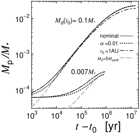
Figure 4: Same as Fig. 3 but with one of the parameters $\alpha$, $M_{0}$, or $r_{0}$ varied from the nominal values for $M_{d}(t_{0})=0.007$ and $0.01M_{*}$. The solid lines represent nominal cases. For dotted lines, $\alpha$ is set to be 0.01. The initial planet mass and orbital radius are five earth masses and 1 AU for gray dashed lines and dot-dashed lines, respectively.

Figure 5: Final planet mass as a function of the initial disk mass $M_{d}(t_{0})$ (solid line) in the case of $\dot{M}_{\mbox{\scriptsize{w}}}=10^{-9}M_{*}/\mbox{yr}$. For comparison, $M_{d}(t_{0})$ (dashed line) and $M_{\mbox{\scriptsize{sup}}}+M_{0}$ (dotted line) are also plotted. The latter is the planet mass when all of the gas supplied from the outer disk perfectly accretes onto the planet. All masses are normalized by $M_{*}$.

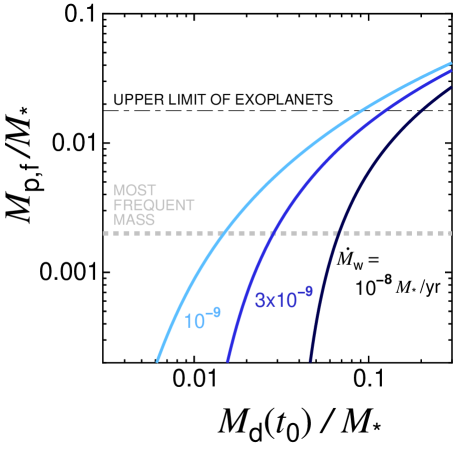
Figure 6: Same as Figure 5 but for various mass loss rates due to photoevaporation, $\dot{M}_{\mbox{\scriptsize{w}}}$. The light blue, blue, and black lines represent the cases with $\dot{M}_{\mbox{\scriptsize{w}}}=10^{-9}$, $3\times 10^{-9}$, and $10^{-8}M_{*}/\mbox{yr}$, respectively. The dot-dashed line is the upper mass limit of exoplanets, and the gray dotted line indicates the most frequent mass of exoplanets in Figure 1.

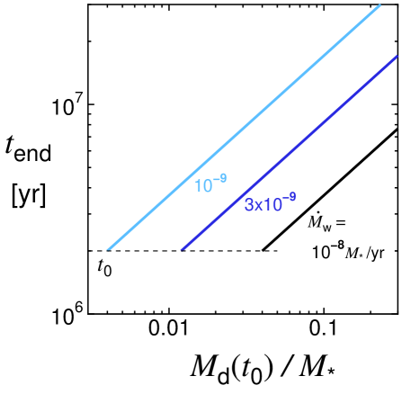
Figure 7: Disk dissipation time, $t_{\mbox{\scriptsize{end}}}$, at the planet-forming region as function of the initial disk mass $M_{d}(t_{0})$ for various mass loss rates.

In Figure 4, we check for the dependence of the time evolution on the parameters $\alpha$, $M_{0}$, and $r_{0}$. As predicted in Section 3.4, we find that the dependence on the viscosity parameter $\alpha$ is slight, especially for $M_{p}>3\times 10^{-4}M_{*}$. The dependence on the initial planet mass $M_{0}$ is also very weak when $M_{p}\gg M_{0}$. The time evolution and the final value of the planet mass is weakly dependent on $r_{0}$ for $M_{p}\gtrsim 10^{-2}M_{*}$. This is because the ratio $D^{\prime}/3\pi\nu$ is proportional to $r_{p}^{1/4}$. Hence, we can say that the dependence of the final planet mass on these parameters is weak. As a result of the independence of $\alpha$, the final planet mass is also approximately independent of the initial disk radius, $R_{d}(t_{0})$, because $R_{d}(t_{0})$ depends on $\alpha$ (see Equations (13) and (18)).

Figure 5 shows the final planet mass as a function of the initial disk mass $M_{d}(t_{0})$ in the case of $\dot{M}_{\mbox{\scriptsize{w}}}=10^{-9}M_{*}/\mbox{yr}$. If all of the gas supplied from the outer disk perfectly accretes onto the planet, the final planet mass is $M_{\mbox{\scriptsize{sup}}}+M_{0}$, where $M_{\mbox{\scriptsize{sup}}}$ is given by Equation (LABEL:msup). This approximate final planet mass is also plotted.

Both lines agree well with each other for $M_{p}\lesssim 10^{-3}M_{*}$ because the assumption of perfect accretion onto the planet is valid for such less massive planets (see Section 3.4). For $M_{p}\gtrsim 10^{-2}M_{*}$, on the other hand, a major part of the gas supplied from the outer disk does not accrete onto the planet but flows to the innermost disk. That is, the accretion onto the planet is imperfect in this case.

Note that, for a much less massive disk with $M_{d}(t_{0})<2t_{0}\dot{M}_{\mbox{\scriptsize{w}}}$ ($=4\times 10^{-3}M_{*}$ in this case), the planet cannot grow through gas accretion because of early gas dissipation at the planet-forming region due to photoevaporation. Then, such a less massive disk produces no giant planet. For $M_{d}(t_{0})=0.01M_{*}$, the final planet mass (or the supplied mass) is only approximately 10% of $M_{d}(t_{0})$. In this case, the disk mass at $t_{\mbox{\scriptsize{end}}}$ is approximately 70% of $M_{d}(t_{0})$ and 20% of $M_{d}(t_{0})$ is dissipated by the photoevaporation.

Figure 6 shows the dependence of the final planet mass on the initial disk mass but for various mass loss rates $\dot{M}_{\mbox{\scriptsize{w}}}$. From this result, we are able to determine how massive a disk is required at $t_{0}$ for each final planet mass. The required disk mass increases with the mass loss rate $\dot{M}_{\mbox{\scriptsize{w}}}$ for a given final planet mass. In these mass loss rates, the final planet mass is always less than or equal to 20% of $M_{d}(t_{0})$. For Jupiter-mass planets ($M_{p}\simeq 10^{-3}M_{*}$), the ratios $M_{p,f}/M_{d}(t_{0})$ are only 10, 5, and 2%, with $\dot{M}_{\mbox{\scriptsize{w}}}=10^{-9}$, $3\times 10^{-9}$, and $10^{-8}M_{*}/$yr, respectively. In Paper 2, we expected that the final planet mass should be comparable to the disk mass at $t_{0}$. This expectation was inaccurate because Paper 2 did not include photoevaporation. Although Paper 2 suggested a much less massive disk than the MMSN disk for the formation of Jupiter, our new model requires the mass (or the surface density) of the MMSN disk for Jupiter because of mass loss due to photoevaporation. Even for massive disks with $M_{d}(t_{0})\sim 0.1M_{*}$, the ratio, $M_{p,f}/M_{d}(t_{0})$, does not increases much because of the imperfect accretion onto massive planets, as shown in Figure 5. Thus, $M_{p,f}/M_{d}(t_{0})$ is always kept small by the mass loss due to photoevaporation and imperfect accretion onto the planet.

Figure 7 shows the disk dissipation time, $t_{\mbox{\scriptsize{end}}}$, for the planet-forming region due to photoevaporation. The disk dissipation time is shortened for a higher mass loss rate $\dot{M}_{\mbox{\scriptsize{w}}}$. For a much lower mass loss rate than $10^{-9}M_{*}/$yr, the disk lifetime is too long ($t_{\mbox{\scriptsize{end}}}\gg 2\times 10^{7}$ yr). Such a weak photoevaporation with a rate of $\leq 3\times 10^{-10}M_{*}/$yr would be inconsistent with the observed disk lifetime. Moreover, too strong photoevaporation with a rate of $\geq 3\times 10^{-8}M_{*}/$yr would be inconsistent. Such strong photoevaporation would dissipate the disk before the planetary cores grow to the critical core mass. Thus, we can say that the mass loss rates in Figure 6 cover the entire reasonable range. This reasonable range of $\dot{M}_{\mbox{\scriptsize{w}}}=10^{-9}$-$10^{-8}M_{*}/$yr is consistent with previous estimations (e.g., Armitage et al. 2003; Mordasini et al. 2009).

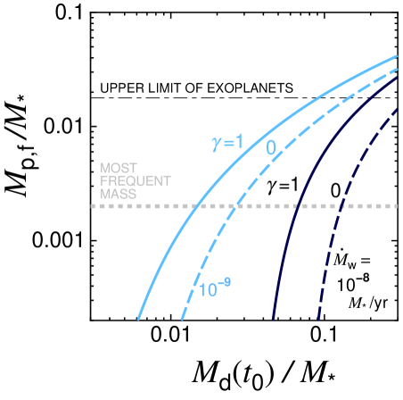
Figure 8: Dependence of the final planet mass on the disk surface density gradient.

Although, thus far, we have assumed $\gamma=1$ (i.e. $\nu\propto r$), we also examine the $\gamma$-dependence of the final planet mass. The index $\gamma$ also determines the radial surface density distribution as $\Sigma\propto r^{-\gamma}$. In Figure 8, we also plot the final planet masses for $\gamma=0$ (i.e., for a flat surface density distribution) as an extreme case. The flat surface density case produces planets with relatively low masses as compared with the case of $\gamma=1$. This is because the disk dissipation is earlier in $\gamma=0$, as shown in Equation (22). Since the case of $\gamma=0$ would be extreme, the $\gamma$-dependence of the final planet mass would not be so significant.

4.2 Which Disks Produce Giant Exoplanets?

With our planet formation model, we can connect the data of giant exoplanets to observed disk masses. In Figure 6, we also plot two reference planet masses, the upper limit mass ($0.018M_{*}$) and most frequent mass ($\simeq 0.002M_{*}$) of giant exoplanets. These masses are obtained from data of exoplanets observed by the radial-velocity methods (in Figure 1).

The required disk mass for the upper limit of exoplanets is 0.1-0.2 $M_{*}$ for the reasonable mass loss rates of $\dot{M}_{\mbox{\scriptsize{w}}}=10^{-9}$-$10^{-8}M_{*}/$ yr. The mass of the most massive observed disk is also $\simeq 0.1M_{*}$. Thus, our model succeeds in reproducing the most massive exoplanets within the observed disk masses and the reasonable disk mass loss rates. It is also expected that exoplanets with the most frequent mass might be produced in disks with the most frequent disk mass, which is $\sim 0.03M_{*}$ for a relatively old star-forming region of $\sim 10^{6}$ yr (Andrews et al. 2010). This indicates that the disk mass loss rate of a few $10^{-9}M_{*}/$yr is plausible for reproducing the most frequent exoplanets in Figure 6.

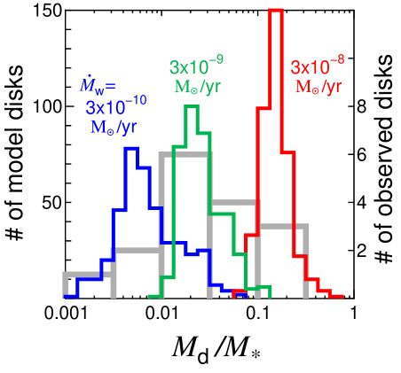
Figure 9: Mass distributions of model disks forming exoplanets observed by the radial velocity survey. The disk masses at $t_{0}$ are estimated using our simple model for $\dot{M}_{\mbox{\scriptsize{w}}}=3\times 10^{-10}$(blue), $3\times 10^{-9}$(green), and $3\times 10^{-8}M_{\odot}/$yr (red). For other parameter settings, see the text. The disk mass is normalized by the mass of the central star. For comparison, we also plot the mass distribution of disks observed in the Ophiuchus star-forming region (gray) given by Andrews et al. (2010).

We also estimate the masses of the disks forming each exoplanet in Figure 1 for a given mass loss rate $\dot{M}_{\mbox{\scriptsize{w}}}$, using our simple model. As for data of exoplanets, we use the planet mass $M_{p}\sin i$, the orbital radius (semi-major axis) $r_{p}$, and the mass of the central star $M_{*}$ obtained from the radial velocity survey data in http://exoplanets.org. We simply put sin $i=$ 1.

We set $M_{0}$, $\alpha$, and $\gamma$ to be nominal values. The estimated disk masses depend primarily on the masses of exoplanets and the mass loss rate $\dot{M}_{\mbox{\scriptsize{w}}}$. As shown in Figure 4, the orbital radii of exoplanets and the parameters of $M_{0}$ and $\alpha$ do not greatly affect the estimation of disk mass. Planets less massive than $M_{0}$ are excluded from our estimations. We consider exoplanets with $r_{p}>0.1$ AU only. Disk mass estimation is performed for three mass loss rates of $\dot{M}_{\mbox{\scriptsize{w}}}=3\times 10^{-10}$, $3\times 10^{-9}$, and $3\times 10^{-8}M_{\odot}/$yr. The starting time of runaway gas accretion onto planets, $t_{0}$, is set to be $2\times 10^{6}$ yr.

Figure 9 shows the distributions of the estimated masses of the disks forming each exoplanet. The disk mass is normalized by the mass of the central star. For comparison, we also plot the mass distribution of disks observed in the Ophiuchus star-forming region obtained by Andrews et al. (2010). Note that the disk masses are normalized by the masses of each central star. The distribution obtained for $\dot{M}_{\mbox{\scriptsize{w}}}=3\times 10^{-9}M_{\odot}/$yr has almost the same peak as the observed disks. In this case, the maximum disk masses in our model (0.13$M_{*}$) and the observation (0.24$M_{*}$) are also close to each other. These results are consistent with Figure 6. The obtained distribution has no disks with $M_{d}<0.9\times 10^{-3}M_{*}$ for $\dot{M}_{\mbox{\scriptsize{w}}}=3\times 10^{-9}M_{\odot}/$yr. This is because giant planets are not formed in less massive disks with $M_{d}(t_{0})<2t_{0}\dot{M}_{\mbox{\scriptsize{w}}}$ ($=0.012M_{\odot}$ in this case) due to early disk dissipation (see Section 3.3). Only planets of Neptune size or less are formed in such disks.

For $\dot{M}_{\mbox{\scriptsize{w}}}=3\times 10^{-8}M_{\odot}/$yr, 90% of disks have masses greater than 0.1$M_{*}$. Some are estimated as $M_{d}>0.5M_{*}$. Thus it is difficult to explain the origin of giant exoplanets with the observed disks under the relatively high mass loss rate of $3\times 10^{-8}M_{\odot}/$yr. For a low mass loss rate of $3\times 10^{-10}M_{\odot}/$yr, on the other hand, the obtained mass distribution has a peak at $5\times 10^{-3}M_{*}$, which is inconsistent with the observed disks. This low mass loss rate also causes a very long disk lifetime of $3\times 10^{7}$yr for massive disks with 0.07$M_{*}$. In addition, from Figure 9, therefore, we can conclude that the mass loss rate of $3\times 10^{-9}M_{\odot}/$yr is plausible to explain giant exoplanets with realistic disks in our simple model.

5 Summary and Discussion

We developed a new model for giant planet formation by including the effect of photoevaporation and a new model for type II planetary migration proposed by Kanagawa et al. (2018). As an effect of photoevaporation, we included disk mass loss with a constant rate outside of the planet orbit. This mass loss dissipates the disk gas at the planet-forming region and terminates planet growth. Our model can predict the final mass of a giant planet produced in a given disk. Our results are summarized as follows.

1. Our simple model gives analytical and universal evolution tracks of planets growing via runaway gas accretion in the mass-orbit diagram (Equation (11) and Figure 1), which are completely independent of disk properties (i.e., the mass, radius, temperature, or viscosity). Planets with a few Jupiter masses or less suffer only a slight radial migration at the runaway gas accretion stage because of their rapid growth. Even the massive exoplanet with $\sim 20M_{J}$ at 3 AU is formed from solid cores initially located within 20 AU. Giant exoplanets crowded around 2 AU can be explained if a large number of massive solid cores are formed from 1.5 AU to 4 AU of protoplanetary disks. Such massive planetary embryos may be formed just outside of the snow line, which is located at 1 to 3 AU.

2. We examined the time evolution and the final mass of a planet, using a simple disk model including the effects of photoevaporation and gas accretion onto the planet. The final planet mass depends primarily on two parameters only (Figure 6). One is the product of the starting time of accretion onto the planet, $t_{0}$, and the mass loss rate due to photoevaporation, and the other is the initial disk mass at $t_{0}$. The final planet mass depends only slightly on the initial disk radius, the viscosity, the initial planet mass, and the initial orbital radius (Figure 4). The mass loss rate due to photoevaporation is a parameter, but is constrained in the range of $10^{-9}$-$10^{-8}M_{*}/$yr by the lifetime of the observed disks (Figure 7).

3. Giant planets grow through the accretion of the disk gas supplied from the outer disk. Planets of Jupiter-mass or less can capture the supplied disk gas almost perfectly. The final masses of such small planets are given by the total supplied mass $M_{\mbox{\scriptsize{sup}}}$ of Equation (LABEL:msup). For massive planets with several Jupiter masses or larger, a major part of the gas passes by the planet and flows into the innermost disk (Figure 5).

4. The ratio of the final planet mass to the initial disk mass at $t_{0}$ is always $\lesssim 0.1$, because of photoevaporation and imperfect accretion onto the planet (Figure 6).

5. With our formation model, we can connect the data of giant exoplanets to the observed disk masses. The most massive exoplanet ($\simeq 20M_{J}$) is born in the most massive T Tauri disk with $M_{d}\sim 0.1M_{*}$ for the reasonable range of mass loss rate due to photoevaporation. Our model also succeeds in explaining the most frequent mass of giant exoplanets ($\sim 2M_{J}$) with the most common disk mass with $\sim 0.02M_{*}$ for a disk mass loss rate of $3\times 10^{-9}M_{\odot}/$yr (Figures 6 and 9). Thus our model successfully explains properties in the mass distribution of giant exoplanets with the observed mass distribution of protoplanetary disks for a reasonable range of the mass loss rate due to photoevaporation.

In our simple model, we focused on the formation of a single giant planet in each protoplanetary disk and did not consider any interaction between multiple planets. Interactions between multiple planets, however, can be important to explain observed giant exoplanets. Due to their gravitational interactions, multiple gas giant systems can be orbitally unstable. The orbital instability of such multiple systems often produces giant planets in eccentric orbits and ejects some planets from the system at the same time (jumping Jupiters model; e.g., Rasio & Ford 1996; Weidenschilling & Marzari 1996; Lin & Ida 1997). Planet-planet scattering followed by tidal circularization can form hot Jupiters with small orbital radii (e.g., Rasio & Ford 1996; Nagasawa et al. 2008; Winn et al. 2010). Since our universal evolution tracks indicate insufficient type II migration for planets of Jupiter-mass or less because of their rapid growth via runaway gas accreion (Figure 1), the scenario of planet-planet scattering would be plausible for hot Jupiters. The type I migration of solid planetary cores before the runaway gas accretion stage can be an alternative possible origin of hot Jupiters since their growth time is expected to be much longer than that at the runaway gas accretion stage.

Indirect interaction through gas accretion onto planets would also be important. We consider multiple giant planets growing by gas accretion. If the outermost giant planet has a Jupiter mass or less, the gas accretion onto the outer planet is almost perfect (Figure 5) and the mass supply to inner planets is significantly reduced. Thus, only the outermost giant planet can grow with gas accretion in this system. When the outermost giant planet has grown to several Jupiter masses or larger, however, its gas accretion becomes imperfect and the inner planets can also grow. Jupiter and Saturn are also expected to have been influenced by such an indirect interaction in their growth stages. Once Saturn starts runaway gas accretion, Jupiter, which is located inside Saturn’s orbit, cannot grow further due to the perfect accretion onto Saturn. Thus, Saturn’s runaway gas accretion should start just after Jupiter had grown to its present mass. Such a formation scenario for Jupiter and Saturn is suggested by our simple model. Both direct and indirect interactions should be included in future formation models for multiple systems of giant planets.

The empirical formula of the gas accretion rate onto a planet used in our model might need to be improved. Our empirical formula of the mass accretion rate has been confirmed by the hydro-dynamic simulations by D’Angelo et al. (2003) and Machida et al. (2010), but only for Jupiter-mass planets or smaller. Only a few hydro-dynamic simulations have been performed for gas accretion onto a giant planet much heavier than Jupiter. Kley & Dirksen (2006) showed through their hydro-dynamical simulations that massive giant planets with masses $\geq 3M_{J}$ strongly excite an eccentric motion of gas at the edge of the planetary gap. Owing to the eccentric motion, the gas accretion rate onto the planet is greatly enhanced in their simulations with the planet masses $\geq 5M_{J}$. On the other hand, Bodenheimer et al. (2013) obtained much lower gas accretion rates than in our formula in their hydro-dynamical simulations with $\geq 3M_{J}$. Further extensive hydro-dynamical simulations on gas accretion onto high-mass giant planets should be performed in order to fix the accretion rate accurately.

The authors would like to thank anonymous referees for valuable comments. The authors also thank Shigeru Ida and Kazuhiro Kanagawa for providing detailed comments. The present study was supported by JSPS KAKENHI grant numbers 17H01103, 18H05438, 19K03941, and 15H02065.

References

- Alexander et al. (2014) Alexander, R.,Pascucci, I.,Andrews, S.,Armitage, P., & Cieza, L. 2014, in Protostars and Planets VI, ed. H. Beuther et al. (Tucson, AZ: Univ. Arizona Press), 475
- Andrews et al. (2010) Andrews, S. M., Wilner, D. J., Hughes, A. M., Qi, C., & Dullemond, C. P. 2010, ApJ, 723, 1241
- Armitage (2007) Armitage, P. J. 2007, ApJ, 665, 1381
- Armitage et al. (2003) Armitage, P. J., Clarke, C. J., & Palla, F. 2003, MNRAS, 342, 1139
- Benz et al. (2014) Benz, W., Ida, S., Alibert, Y., Lin, D., & Mordasini, C. 2014, in Protostars and Planets VI, ed. H. Beuther et al. (Tucson, AZ: Univ. Arizona Press), 691
- Bitsch et al. (2015) Bitsch, B., Lambrechts, M., & Johansen, A. 2015, A&A, 582, 112
- Bitsch et al. (2019) Bitsch, B., Izidoro, A., Johansen, A., Raymond, S. N., et al. 2019, A&A, 623, 88
- Bodenheimer et al. (2013) Bodenheimer, P., D’Angelo, G., Lissauer, J. J., Fortney, J. J., & Saumon, D. 2013, ApJ, 770, 120
- Clarke et al. (2001) Clarke, C. J., Gendrin, A., & Sotomayer, M. 2001, MNRAS, 328, 48
- Crida et al. (2006) Crida, A., Morbidelli, A., & Masset, F. 2006, Icarus, 181, 587
- D’Angelo et al. (2003) D’Angelo, G., Kley, W., & Henning, T. 2003, ApJ, 586, 540
- D’Angelo & Lubow (2008) D’Angelo, G., & Lubow, S. H. 2008, ApJ, 685, 560
- Duffell et al. (2014) Duffell, P. C., Haiman, Z., MacFadyen, A. I., D’Orazio, D. J., & Farris, B. D. 2014, ApJ, 792, 10
- Duffell & MacFadyen (2013) Duffell, P. C., & MacFadyen, A. I. 2013, ApJ, 769, 41
- Dürmann & Kley (2015) Dürmann, C., & Kley, W. 2015, A&A, 574, A52
- Dürmann & Kley (2017) Dürmann, C., & Kley, W. 2017, A&A, 598, 80
- Fung et al. (2014) Fung, J., Shi, J., & Chiang, E. 2014, ApJ, 782, 88
- Ginzburg & Chiang (2019) Ginzburg, S., & Chiang, E. 2019, MNRAS, 487, 681
- Gorti & Hollenbach (2009) Gorti, U., Hollenbach, D. 2009, ApJ, 690, 1539
- Hubickyj et al. (2005) Hubickyj, O., Bodenheimer, P., & Lissauer, J. J. 2005, Icarus, 179, 415
- Hartmann et al. (1998) Hartmann, L., Calvet, N., Gullbring, E., & D’Alessio, P. 1998, ApJ, 495, 385
- Hasegawa & Ida (2013) Hasegawa, Y., & Ida, S. 2013, ApJ, 774, 146
- Hayashi et al. (1985) Hayashi, C., Nakazawa, K., & Nakagawa, Y. 1985, in Protostars and Planets II, ed. D. C. Black, & M. S. Matthews (Tucson, AZ: Univ. Arizona Press), 1100
- Ida & Lin (2004) Ida, S., & Lin, D. N. C. 2004, ApJ, 604, 388
- Ida et al. (2018) Ida, S.,Tanaka, H., Johansen, A., Kanagawa, K. D., & Tanigawa T. 2018, ApJ, 864, 77
- Ikoma et al. (2000) Ikoma, M., Nakazawa, K., & Emori, H. 2000, ApJ, 537, 1013
- Johansen et al. (2019) Johansen, A., Ida, S., & Brasser, R. 2019, A&A, 622, 202
- Kanagawa et al. (2015a) Kanagawa, K. D., Muto, T., Tanaka, H., Tanigawa, T., & Takeuchi, T. 2015a, MNRAS, 448, 994
- Kanagawa et al. (2015b) Kanagawa, K. D., Tanaka, H., Muto, T., Tanigawa, T., et al. 2015b, ApJ, 806, L15
- Kanagawa et al. (2016) Kanagawa, K. D., Muto, T., Tanaka, H., Tanigawa, T., et al. 2016, PASJ, 68, 43
- Kanagawa et al. (2017) Kanagawa, K. D., Tanaka, H., Muto, T., & Tanigawa, T. 2017, PASJ, 69, 97
- Kanagawa et al. (2018) Kanagawa, K. D., Tanaka, H., & Szuszkiewicz, E. 2018, ApJ, 861, 140
- Kley (1999) Kley, W. 1999, MNRAS, 303, 696
- Kley & Dirksen (2006) Kley, W., & Dirksen, G. 2006, A&A, 447, 369
- Kokubo & Ida (2002) Kokubo, E., & Ida, S. 2002, ApJ, 581, 666
- Lambrechts & Johansen (2014) Lambrechts, M., & Johansen, A. 2014, A&A, 572, 107
- Lambrechts et al. (2019) Lambrechts, M., Lega, E.; Nelson, R. P., Crida, A., & Morbidelli, A. 2019, A&A, 630, 82
- Lin & Ida (1997) Lin, D. N. C., & Ida, S. 1997, ApJ, 477, 781
- Lin & Papaloizou (1986) Lin, D. N. C., & Papaloizou, J. 1986, ApJ, 309, 846
- Lin & Papaloizou (1993) Lin, D. N. C., & Papaloizou, J. 1993, in Protostars and Planets III, ed. E. H. Levy & J. Lunine (Tucson, AZ: Univ. Arizona Press), 749
- Lin et al. (1996) Lin, D. N. C., Bodenheimer, P., & Richardson, D. C. 1996, Nature, 380, 606
- Lubow et al. (1999) Lubow, S. H., Seibert, M., & Artymowicz, P. 1999, ApJ, 526, 1001
- Lubow & D’Angelo (2006) Lubow, S. H., & D’Angelo, G. 2006, ApJ, 641, 526
- Lynden-Bell & Pringle (1974) Lynden-Bell, D., & Pringle, J. E. 1974, MNRAS, 168, 603
- Machida et al. (2010) Machida, N. M., Kokubo, E., Inutsuka, S., & Matsumoto, T. 2010, MNRAS, 405, 1227
- Masset & Snellgrove (2001) Masset, F., & Snellgrove, M. 2001, MNRAS, 320, L55
- Masset & Papaloizou (2003) Masset, F., & Papaloizou, J. C. B. 2003, ApJ, 588, 494
- Mizuno (1980) Mizuno, H. 1980, PThPh, 64, 544
- Mordasini et al. (2009) Mordasini, C., Alibert, Y., & Benz, W. 2009, A&A, 501, 1139
- Movshovitz & Podolak (2008) Movshovitz, N., Podolak, M. 2008, Icarus, 194, 36
- Nagasawa et al. (2008) Nagasawa, M., Ida, S., & Bessho, T. 2008, ApJ, 678, 498
- Paardekooper et al. (2011) Paardekooper, S.-J., Baruteau, C., & Kley, W. 2011, MNRAS, 410, 293
- Paardekooper (2014) Paardekooper, S.-J. 2014, MNRAS, 444, 2031
- Pierens & Raymond (2016) Pierens, A., & Raymond, S. N. 2016, MNRAS, 462, 4130
- Pollack et al. (1996) Pollack, J. B., Hubickyj, O., Bodenheimer, P., Lissauer, J. J. et al. 1996, Icarus, 124, 62
- Rasio & Ford (1996) Rasio, F., & Ford, E. 1996, Science, 274, 954
- Robert et al. (2018) Robert, C. M. T., Crida, A., Lega, E., Méheut, H., & Morbidelli, A. 2018, A&A, 617, 98
- Shakura & Sunyaev (1973) Shakura, N. I., & Sunyaev, R. A. 1973, A&A, 24, 337
- Tanaka et al. (2002) Tanaka, H., Takeuchi, T., & Ward, W. R. 2002, ApJ, 565, 1257
- Tanigawa& Ikoma (2007) Tanigawa, T. & Ikoma, M. 2007, ApJ, 667, 557 (Paper 1)
- Tanigawa& Tanaka (2016) Tanigawa, T. & Tanaka, H. 2016, ApJ, 823, 48 (Paper 2)
- Tanigawa& Watanabe (2002) Tanigawa, T. & Watanabe, S. 2002, ApJ, 586, 506
- Weidenschilling & Marzari (1996) Weidenschilling, S. J., & Marzari, F. 1996, Nature, 384, 619
- Winn et al. (2010) Winn, J. N., Fabrycky, D., Albrecht, S., & Johnson, J. A. 2010, ApJ, 718, L145
- Zhu et al. (2011) Zhu, Z., Nelson, R. P., Hartmann, L., Espaillat, C., Calvet, N. 2011, ApJ, 729, 47