A Note on Costs Minimization with Stochastic Target Constraints

Abstract.

We study the minimization of the expected costs under stochastic constraint at the terminal time. The first and the main result says that for a power type of costs, the value function is the minimal positive solution of a second order semi–linear ordinary differential equation (ODE). Moreover, we establish the optimal control. In the second example we show that the case of exponential costs leads to a trivial optimal control.

1. Introduction and Main Results

This note was inspired by a series of papers which dealt with stochastic tracking problems; see, e.g., [1, 2, 3, 4, 5, 6, 7, 8, 10] and the references therein.

Consider a complete probability space $(\Omega,\mathcal{F},\mathbb{P})$ together with a standard one–dimensional Brownian motion $W_{t},t\geq 0$ and the Brownian filtration $\mathcal{F}^{W}_{t}:=\sigma\{W_{u}:u\leq t\}$ completed by the null sets.

For any $(T,x)\in(0,\infty)\times\mathbb{R}$ and a progressively measurable processes $u=\{u_{t}\}_{t=0}^{T}$ which satisfies the integrability condition $\int_{0}^{T}|u_{t}|dt<\infty$ a.s. we denote

$$X^{x,u}_{t}:=x+\int_{0}^{t}u_{s}ds,\ \ t\in[0,T].$$

For any $(T,x,c)\in(0,\infty)\times\mathbb{R}^{2}$ let $U(T,x,c)$ be the set of all progressively measurable processes $u=\{u_{t}\}_{t=0}^{T}$ (with the above integrability condition) which satisfy $X^{x,u}_{T}\geq\mathbb{I}_{W_{T}>c}$ a.s. As usual, we set $\mathbb{I}_{Q}=1$ if an event $Q$ occurs and $\mathbb{I}_{Q}=0$ if not.

For a given $p>1$ introduce the stochastic control problem

(1.1) $$v(T,x,c):=\inf_{u\in U(T,x,c)}\mathbb{E}\left[\int_{0}^{T}|u_{t}|^{p}dt\right].$$

For a given $(T,x,c)\in(0,\infty)\times[0,1]\times\mathbb{R}$ we say that $u\in U(T,x,c)$ is optimal if $\mathbb{E}[\int_{0}^{T}|u_{t}|^{p}dt]=v(T,x,c).$ Let $U^{+}(T,x,c)\subset U(T,x,c)$ be the set of all $u\in U(T,x,c)$ such that $u\geq 0$ $dt\otimes\mathbb{P}$ a.s. and $X^{x,u}_{T}\leq 1$ a.s.

Lemma 1.1.

For any $(T,x,c)\in(0,\infty)\times[0,1]\times\mathbb{R}$

$$v(T,x,c)=\inf_{u\in U^{+}(T,x,c)}\mathbb{E}\left[\int_{0}^{T}|u_{t}|^{p}dt\right].$$

Proof.

Let $u\in U(T,x,c)$. Define

$$\hat{u}_{t}:=\max(0,u_{t}),\ \ t\in[0,T],$$

$$\theta:=T\wedge\inf\{t:X^{x,\hat{u}}_{T}=1\},$$

and

$$\tilde{u}_{t}:=\hat{u}_{t}\mathbb{I}_{t<\theta},\ \ t\in[0,T].$$

Observe that,

$$X^{x,\tilde{u}}_{T}\geq 1\wedge X^{x,u}_{T}\geq\mathbb{I}_{W_{T}>c}$$

and

$$\mathbb{E}\left[\int_{0}^{T}|\tilde{u}_{t}|^{p}dt\right]\leq\mathbb{E}\left[\int_{0}^{T}|u_{t}|^{p}dt\right].$$

This completes the proof. ∎

The following Proposition will be crucial for deriving the main results.

Proposition 1.2.

For any $(T,x,c)\in(0,\infty)\times[0,1]\times\mathbb{R}$

$$v(T,x,c)=\frac{(1-x)^{p}}{T^{p-1}}v\left(1,0,\frac{c}{\sqrt{T}}\right).$$

Proof.

The statement is obvious for $x=1$. Thus assume that $x<1$.

We use the scaling property of Brownian motion. Define the Brownian motion $B_{t}:=\frac{W_{tT}}{\sqrt{T}}$, $t\geq 0$. Let $\mathcal{F}^{B}_{t}:=\sigma\{B_{u}:u\leq t\}$ be the filtration generated by $B$ completed with the null sets. Clearly, $\mathcal{F}^{B}_{t}=\mathcal{F}^{W}_{tT}$, $t\geq 0$. Let $\tilde{U}$ be the set of all stochastic processes $\tilde{u}=\{\tilde{u}_{t}\}_{t=0}^{1}$ which are non negative, progressively measurable with respect to $\mathcal{F}^{B}$ and satisfy

$$\mathbb{I}_{B_{1}>\frac{c}{\sqrt{T}}}\leq\int_{0}^{1}\tilde{u}_{t}dt\leq 1.$$

We notice that there is a bijection $U^{+}(T,x,c)\leftrightarrow\tilde{U}$ which is given by

$$u_{t}=\frac{(1-x)\tilde{u}_{\frac{t}{T}}}{T},\ t\in[0,T].$$

Thus, from Lemma 1.1

$$v(T,x,c)=\min_{u\in U^{+}(T,x,c)}\mathbb{E}\left[\int_{0}^{T}u^{p}_{t}dt\right]$$

$$=\min_{\tilde{u}\in\tilde{U}}\frac{(1-x)^{p}}{T^{p-1}}\mathbb{E}\left[\int_{0}^{1}\tilde{u}^{p}_{t}dt\right]=\frac{(1-x)^{p}}{T^{p-1}}v\left(1,0,\frac{c}{\sqrt{T}}\right).$$

∎

Next, let $\Phi(\cdot)=\frac{1}{\sqrt{2}\pi}\int_{-\infty}^{\cdot}e^{-\frac{y^{2}}{2}}dy$ be the cumulative distribution function of the standard normal distribution. For any $T>0$ and $c\in\mathbb{R}$ consider the martingale $\{M^{T,c}_{t}\}_{t=0}^{T}$ given by

(1.2) $$M^{T,c}_{T}=\mathbb{I}_{W_{T}<c},\ \ M^{T,c}_{t}=\mathbb{P}(W_{T}<c|\mathcal{F}^{W}_{t})=\Phi\left(\frac{c-W_{t}}{\sqrt{T-t}}\right),\ t\in[0,T).$$

Define the function $g:(0,1)\rightarrow\mathbb{R}_{+}$ by

$$g(z)=v\left(1,0,\Phi^{-1}(z)\right)$$

where $\Phi^{-1}$ is the inverse function. From Proposition 1.2 we have

(1.3) $$v(t,x,c)=\frac{(1-x)^{p}}{t^{p-1}}g\left(\Phi\left(\frac{c}{\sqrt{t}}\right)\right)=\frac{(1-x)^{p}}{t^{p-1}}g(M^{t,c}_{0}),\ \ \forall(t,x,c)\in(0,\infty)\times[0,1]\times\mathbb{R}.$$

Now, we are ready to state the main results which will be proved in Section 2.

Theorem 1.3.

(I) Let $h:(0,1)\rightarrow\mathbb{R}_{+}$ be given by $h(y)=\frac{\exp\left(-[\Phi^{-1}(y)]^{2}\right)}{4\pi}.$ The function $g:(0,1)\rightarrow\mathbb{R}_{+}$ is a non increasing solution of the ODE

(1.4) $$h(y)g^{\prime\prime}(y)+(p-1)\left(g(y)-g^{\frac{p}{p-1}}(y)\right)=0,\ \ y\in(0,1)$$

with the boundary conditions

(1.5) $$\lim_{y\rightarrow 0}g(y)=1\ \mbox{and}\ \lim_{y\rightarrow 1}g(y)=0.$$

Moreover, the following minimality holds. If $\hat{g}:(0,1)\rightarrow\mathbb{R}_{+}$ is another solution to (1.4) ($\hat{g}(y_{0})\neq g(y_{0})$ for some $y_{0}$) and satisfies

(1.6) $$\lim_{y\rightarrow 0}\hat{g}(y)>0$$

then $\hat{g}(y)>g(y)$ for all $y\in(0,1)$.
(II) Let $(T,x,c)\in(0,\infty)\times[0,1]\times\mathbb{R}$. The optimal control is given by

$$\hat{u}_{t}=(1-x)\frac{g^{\frac{1}{p-1}}(M^{T,c}_{t})}{T-t}\exp\left(-\int_{0}^{t}\frac{g^{\frac{1}{p-1}}(M^{T,c}_{s})}{T-s}ds\right),\ \ \ t\in[0,T).$$

Namely, for the optimal control we have the ODE:

$$\frac{dX^{x,\hat{u}}_{t}}{dt}=g^{\frac{1}{p-1}}(M^{T,c}_{t})\frac{1-X^{x,\hat{u}}_{t}}{T-t},\ \ \ t\in[0,T).$$

(III) Let $T>0$ and $c\in\mathbb{R}$. Then the pair $(Y,Z)$ given by

$$Y_{t}:=\frac{g(M^{T,c}_{t})}{(T-t)^{p-1}},\ \ Z_{t}:=-\frac{g^{\prime}(M^{T,c}_{t})e^{-\frac{(c-W_{t})^{2}}{2(T-t)}}}{\sqrt{2\pi(T-t)^{2p-1}}},\ \ t\in[0,T)$$

is the minimal solution of the backward stochastic differential equation (BSDE)

(1.7) $$dY_{t}=(p-1)Y^{\frac{p}{p-1}}_{t}dt+Z_{t}dW_{t},\ \ t\in[0,T)$$

with the singular terminal condition $Y_{T}=\infty\mathbb{I}_{W_{T}>c}$. This terminal condition means that $\lim_{t\rightarrow T}Y_{t}=\infty\mathbb{I}_{W_{T}>c}$ a.s. where we use the convention $\infty\cdot 0:=0$.

Remark 1.4.

It is easy to see that the optimal control is unique. Indeed, if by contradiction $u,\tilde{u}\in U(T,x,c)$ are optimal controls and $dt\otimes\mathbb{P}(u\neq\tilde{u})>0$. Then, the process $\frac{u+\tilde{u}}{2}$ satisfies $\frac{u+\tilde{u}}{2}\in U(T,x,c)$ and from the strict convexity of the function $z\rightarrow|z|^{p}$ we have

$$\mathbb{E}\left[\int_{0}^{T}\left|\frac{u_{t}+\tilde{u}_{t}}{2}\right|^{p}dt\right]<\frac{1}{2}\left(\mathbb{E}\left[\int_{0}^{T}|u_{t}|^{p}dt\right]+\mathbb{E}\left[\int_{0}^{T}|\tilde{u}_{t}|^{p}dt\right]\right)=v(T,x,c)$$

which is a contradiction.

Remark 1.5.

A natural question is whether there exists a unique positive, non increasing solution to the ODE (1.4) with the boundary conditions (1.5). Due to the fact that $h$ takes the value $0$ at the end points $\{0,1\}$ the uniqueness seems to be far from obvious and we leave it for future research.

2. Proof of the Main Results

We start with the following regularity result.

Lemma 2.1.

The function $g:(0,1)\rightarrow\mathbb{R}_{+}$ is concave, non increasing and satisfies $\lim_{y\rightarrow 0}g(y)=1$.

Proof.

The fact that $g$ is non increasing is obvious.

Next, we establish the equality $\lim_{y\rightarrow 0}g(y)=1$. From the Jensen inequality it follows that for any $u\in U(1,0,c)$

$$\mathbb{E}\left[\int_{0}^{1}|u_{t}|^{p}dt\right]\geq(\mathbb{P}(W_{1}>c))^{p}=(1-\Phi(c))^{p}.$$

Thus, $g(y)=v(1,0,\Phi^{-1}(y))\geq(1-y)^{p}$ and we conclude that $\lim_{y\rightarrow 0}g(y)=1$.

It remains to prove concavity. Fix $a_{1}<a<a_{2}$. Let us show that

$$g(a)\geq g(a_{1})\frac{a_{2}-a}{a_{2}-a_{1}}+g(a_{2})\frac{a-a_{1}}{a_{2}-a_{1}}.$$

Let $c=\Phi^{-1}(a)$. Choose $\epsilon>0$. There exists $u\in U^{+}(1,0,c)$ such that

(2.1) $$g(a)>\mathbb{E}\left[\int_{0}^{1}|u_{t}|^{p}dt\right]-\epsilon.$$

Consider the martingale $M:=M^{1,c}$ given by (1.2). Observe that $M_{0}=a$. Define the stopping time

$$\tau=\inf\{t:M_{t}\notin(a_{1},a_{2})\}.$$

Clearly, $\tau<1$ a.s. and so from the equality $\mathbb{E}[M_{\tau}]=M_{0}$ we conclude that

(2.2) $$\mathbb{P}(M_{\tau}=a_{1})=\frac{a_{2}-a}{a_{2}-a_{1}}\ \mbox{and}\ P(M_{\tau}=a_{2})=\frac{a-a_{1}}{a_{2}-a_{1}}.$$

Next, let $D=\int_{0}^{\tau}u_{t}dt$. From the Holder inequality

(2.3) $$\int_{0}^{\tau}|u_{t}|^{p}dt\geq\frac{D^{p}}{\tau^{p-1}}\ \ \mbox{a.s.}$$

From (1.3), the fact that $\{W_{s+\tau}-W_{\tau}\}_{s=0}^{\infty}$ is a Brownian motion independent of $\mathcal{F}^{W}_{\tau}$, and the inequality $D+\int_{\tau}^{1}u_{t}dt\geq\mathbb{I}_{W_{1}-W_{\tau}>c-W_{\tau}}$ (notice that $D\in[0,1]$) we get

$$\mathbb{E}\left[\int_{\tau}^{1}|u_{t}|^{p}dt\big{|}\mathcal{F}^{W}_{\tau}\right]\geq v\left(1-\tau,D,c-W_{\tau}\right)$$

$$=\frac{\left(1-D\right)^{p}}{(1-\tau)^{p-1}}g\left(\Phi\left(\frac{c-W_{\tau}}{\sqrt{1-\tau}}\right)\right)=\frac{\left(1-D\right)^{p}}{(1-\tau)^{p-1}}g(M_{\tau}).$$

Thus,

(2.4) $$\mathbb{E}\left[\int_{\tau}^{1}|u_{t}|^{p}dt\right]\geq\mathbb{E}\left[\frac{\left(1-D\right)^{p}}{(1-\tau)^{p-1}}g(M_{\tau})\right].$$

By combining (2.1)–(2.4), the fact that $g\leq 1$ and the simple inequality $\frac{z^{p}}{y^{p-1}}+\frac{(1-z)^{p}}{(1-y)^{p-1}}\geq 1$ for $0<y,z<1$ we obtain

$$g(a)+\epsilon>\mathbb{E}\left[\int_{0}^{1}|u_{t}|^{p}dt\right]\geq\mathbb{E}\left[\left(\frac{D^{p}}{\tau^{p-1}}+\frac{\left(1-D\right)^{p}}{(1-\tau)^{p-1}}\right)g(M_{\tau})\right]$$

$$\geq\mathbb{E}[g(M_{\tau})]=g(a_{1})\frac{a_{2}-a}{a_{2}-a_{1}}+g(a_{2})\frac{a-a_{1}}{a_{2}-a_{1}}.$$

Since $\epsilon>0$ was arbitrary we complete the proof. ∎

The proof of the main results will be based on the theory developed in [8]. We start with preparations. For any $(T,x,c)\in(0,\infty)\times[0,1]\times\mathbb{R}$ introduce the optimal position targeting problem

$$\hat{v}(T,x,c):=\inf_{u}\mathbb{E}\left[\int_{0}^{T}|u_{t}|^{p}dt+\xi|X^{x,u}_{T}|^{p}\right]$$

where the infimum is taken over all progressively measurable processes $u=\{u_{t}\}_{t=0}^{T}$, $\xi:=\infty\mathbb{I}_{W_{T}>c}$ and as before, we use the convention $\infty\cdot 0:=0$.

Using same arguments as in Lemma 1.1 gives that

$$\hat{v}(T,x,c)=\inf_{u\in\hat{U}^{-}(T,x,c)}\mathbb{E}\left[\int_{0}^{T}|u_{t}|^{p}dt+\xi|X^{x,u}_{T}|^{p}\right]$$

where $\hat{U}^{-}(T,x,c)$ is the set of all progressively measurable processes $u=\{u_{t}\}_{t=0}^{T}$ such that $u\leq 0$ $dt\otimes\mathbb{P}$ a.s., $X^{x,u}_{T}\geq 0$ a.s. and $X^{x,u}_{T}=0$ on the event $\{W_{T}>c\}$.

Clearly, there is a bijection $U^{+}(T,x,c)\leftrightarrow\hat{U}^{-}(T,1-x,c)$ given by $u\leftrightarrow-u$. Moreover, for any $u\in U^{-}(T,1-x,c)$ we have

(2.5) $$\mathbb{E}\left[\int_{0}^{T}|-u_{t}|^{p}dt\right]=\mathbb{E}\left[\int_{0}^{T}|u_{t}|^{p}dt+\xi|X^{1-x,u}_{T}|^{p}\right].$$

Thus, from Lemma 1.1 we conclude that

(2.6) $$v(t,x,c)=\hat{v}(t,1-x,c),\ \ \ \forall(t,x,c)\in(0,\infty)\times[0,1]\times\mathbb{R}.$$

This brings us to the following corollary.

Corollary 2.2.

Let $T>0$ and $c\in\mathbb{R}$. There exists a progressively measurable process $\{Z_{t}\}_{0\leq t<T}$ such that the pair $\left(\frac{g(M^{T,c}_{t})}{(T-t)^{p-1}},Z_{t}\right)_{0\leq t<T}$ is the minimal supersolution (see Definition 1 in [8]) to the BSDE given by (1.7) with the singular terminal condition $Y_{T}=\infty\mathbb{I}_{W_{T}>c}$.

Proof.

From Theorem 3 in [8] it follows that there exists a minimal supersoution $(Y,Z)$ to the above BSDE. Moreover, by combining Theorem 3 in [8] together with the Markov property of Brownian motion, (1.3) and (2.6) we obtain that $Y_{t}=\frac{g(M^{T,c}_{t})}{(T-t)^{p-1}}$, $t\in[0,T)$. ∎

Remark 2.3.

A priori we do not know that $g$ is continuously differentiable and so we can not apply the Ito formula and find $Z$. In the proof of Theorem 1.3 we will show that $g$ satisfies the ODE (1.4) and then we will find $Z$.

Now, we are ready to prove Theorem 1.3.

Proof.

Proof of Theorem 1.3.

First step: Proving that the minimal supersolution is a solution.
Fix $T>0$ and $c\in\mathbb{R}$. Let $\xi:=\infty\mathbb{I}_{W_{T}>c}$. Let us show that the supersolution $(Y,Z)$ from Corollary 2.2 is actually a solution. To that end, we need to establish the inequality $\lim\sup_{t\rightarrow T}Y_{t}\leq\xi$.

We wish to apply Theorem 4 in [9]. There is a technical problem that the indicator function is not continuous and so condition (4) in [9] does not hold. Still, this issue can be simply solved by the following density argument. Define a sequence of functions $\phi^{(n)}:\mathbb{R}\rightarrow\mathbb{R}\cup\{\infty\}$, $n\in\mathbb{N}$ by

$$\phi^{(n)}(z)=\left(\frac{1}{c-z}-n\right)\mathbb{I}_{c-\frac{1}{n}\leq z<c}+\infty\mathbb{I}_{z\geq c}.$$

Observe that for any $n$, $\phi^{(n)}$ satisfies condition (4) in [9]. Hence, from Theorem 4 in [9] there exists a pair $(Y^{(n)},Z^{(n)})$ which satisfies the BSDE (1.7) with the terminal constraint $Y^{(n)}_{T}=\phi^{(n)}(W_{T})$. Since $\phi^{(n)}(W_{T})\geq\xi$, then from the minimality property of $(Y,Z)$ we obtain that for any $n$, $Y_{t}\leq Y^{(n)}_{t}$ a.s. for any $t\in[0,T)$. Thus,

$$\lim\sup_{t\rightarrow T}Y_{t}\leq\lim\inf_{n\rightarrow\infty}Y^{(n)}_{T}=\lim_{n\rightarrow\infty}\phi^{(n)}(W_{T})=\xi,$$

as required.

Second step: Establishing statement (I) in Theorem 1.3.
From Corollary 2.2 and the previous step it follows that $\lim_{t\rightarrow 1}\frac{g(M^{1,0}_{t})}{(1-t)^{p-1}}=0$ on the event $\{W_{1}<0\}$. Clearly, $\lim_{t\rightarrow 1}M^{1,0}_{t}=1$ on the event $\{W_{1}<0\}$, and so we conclude that $\lim_{y\rightarrow 1}g(y)=0.$ This together with the boundary condition $\lim_{y\rightarrow 0}g(y)=1$ (was established in Lemma 2.1) gives (1.5).

Next, we prove (1.4). Extend the function $g$ to the closed interval $[0,1]$ by $g(0):=1$ and $g(1):=0$. Choose $a\in(0,1)$. Let $c=\Phi^{-1}\left(\frac{a}{2}\right)$. Consider the martingale $M:=M^{1,c}$. From Lemma 2.1 it follows that $g:[0,1]\rightarrow[0,1]$ is concave and continuous. Thus, $g(M_{t})$, $t\in[0,1]$ is a continuous and uniformly integrable super–martingale. From Doob’s decomposition

$$g(M_{t})=N_{t}-A_{t},\ \ t\in[0,1]$$

where $N=\{N_{t}\}_{t=0}^{1}$ is a martingale and $A=\{A_{t}\}_{t=0}^{1}$ is a continuous, non decreasing process with $A_{0}=0$.

Recall the minimal supersolution $\left(\frac{g(M_{t})}{(1-t)^{p-1}},Z_{t}\right)_{0\leq t<1}$ from Corollary 2.2. From the product rule and (1.7) we get

$$(p-1)\frac{g^{\frac{p}{p-1}}(M_{t})}{(1-t)^{p}}dt+Z_{t}dW_{t}=d\left(\frac{g(M_{t})}{(1-t)^{p-1}}\right)$$

$$=\frac{dN_{t}}{(1-t)^{p-1}}-\frac{dA_{t}}{(1-t)^{p-1}}+(p-1)\frac{g(M_{t})}{(1-t)^{p}}dt.$$

Hence,

$$\frac{dA_{t}}{dt}=(p-1)\frac{g(M_{t})-g^{\frac{p}{p-1}}(M_{t})}{1-t}.$$

We conclude that,

(2.7) $$g(M_{t})=N_{t}-(p-1)\int_{0}^{t}\frac{g(M_{s})-g^{\frac{p}{p-1}}(M_{s})}{1-s}ds\ \ \forall t\in[0,1]\ \ \mathbb{P}\ \mbox{a.s.}$$

Next, observe that $M_{0}=\frac{a}{2}$ and define the function $f:\left[\frac{a}{3},\frac{1+a}{2}\right]\rightarrow\mathbb{R}$ by

$$f(y)=-(p-1)\int_{\beta=a/3}^{y}\int_{\alpha=\frac{a}{3}}^{\beta}\frac{g(\alpha)-g^{\frac{p}{p-1}}(\alpha)}{h(\alpha)}d\alpha d\beta.$$

Notice that $f\in C^{2}\left[\frac{a}{3},\frac{1+a}{2}\right]$ and $f^{\prime\prime}(y)=-(p-1)\frac{g(y)-g^{\frac{p}{p-1}}(y)}{h(y)}$, $y\in\left[\frac{a}{3},\frac{a+1}{2}\right]$.

For any $y\in\left(M_{0},\frac{1+a}{2}\right)$ consider the stopping time $\tau_{y}=\inf\{t:M_{t}\notin\left(\frac{a}{3},y\right)\}$. Clearly, $\tau_{y}<T$ a.s.

We notice that $\frac{d\langle M\rangle}{dt}=\frac{2h(M_{t})}{1-t}$, and so from the Ito Formula and (2.7) we obtain

$$g(M_{\tau_{y}})-f(M_{\tau_{y}})=N_{\tau_{y}}-f(M_{0})-\int_{0}^{\tau_{y}}f^{\prime}(M_{t})dM_{t}.$$

Hence,

(2.8) $$\mathbb{E}[g(M_{\tau_{y}})]-\mathbb{E}[f(M_{\tau_{y}})]=g(M_{0})-f(M_{0}).$$

Similarly, to (2.2)

$$\mathbb{P}(M_{\tau_{y}}=y)=\frac{M_{0}-\frac{a}{3}}{y-\frac{a}{3}}\ \mbox{and}\ \mathbb{P}\left(M_{\tau_{y}}=\frac{a}{3}\right)=\frac{y-M_{0}}{y-\frac{a}{3}}.$$

This together with (2.8) yields that $g(y)-f(y)$ is a linear function on the interval $\left(M_{0},\frac{1+a}{2}\right)$. In particular

$$g^{\prime\prime}(a)=f^{\prime\prime}(a)=-(p-1)\frac{g(a)-g^{\frac{p}{p-1}}(a)}{h(a)}.$$

Since $a\in(0,1)$ was arbitrary we complete the proof of (1.4).

Finally, we prove minimality. Assume that there exists a positive function $\hat{g}\neq g$ which satisfies (1.4) and (1.6). Define the pair $(\hat{Y},\hat{Z})$ by

$$\hat{Y}_{t}:=\frac{\hat{g}(M^{1,0}_{t})}{(1-t)^{p-1}},\ \ \hat{Z}_{t}:=-\frac{\hat{g}^{\prime}(M^{1,0}_{t})e^{-\frac{W^{2}_{t}}{2(1-t)}}}{\sqrt{2\pi(1-t)^{2p-1}}},\ \ t\in[0,1).$$

From the Ito formula ($\hat{g}$ satisfies (1.4) and so continuously differentiable) it follows that the pair $(\hat{Y},\hat{Z})$ is a supersolution to the BSDE (1.7) with the singular terminal condition $\hat{Y}_{T}=\infty\mathbb{I}_{W_{1}>0}$. From Corollary 2.2 we conclude that $\frac{\hat{g}(M^{1,0}_{t})}{(1-t)^{p-1}}\geq\frac{g(M^{1,0}_{t})}{(1-t)^{p-1}}$ a.s. for any $t\in[0,1)$. Thus, $g(y)\geq\hat{g}(y)$ for all $y\in(0,1)$.

Let us argue strict inequality. Indeed, assume by contradiction that there is $y_{0}\in(0,1)$ for which $\hat{g}(y_{0})=g(y_{0})$, then clearly $y_{0}$ is a minimum point for the function $\hat{g}-g$. Hence, $\hat{g}^{\prime}(y_{0})=g^{\prime}(y_{0})$. Since $h(y)$ is bounded away from zero if $y$ is bounded away from the end points $\{0,1\}$, then from standard uniqueness for initial value problems we conclude that $\hat{g}=g$ on the interval $(0,1)$. This is a contradiction and the proof of (I) is completed.

Third step: Completion of the proof.
In this step we complete the proof of statements (II)–(III) in Theorem 1.3. Since $g$ is continuously differentiable (satisfies (1.4)) then from the Ito formula, Corollary 2.2 and the first step of the proof we obtain statement (III).

It remains to prove Statement (II). Let $(T,x,c)\in(0,\infty)\times[0,1]\times\mathbb{R}$ and let $\xi:=\infty\mathbb{I}_{W_{T}>c}$. From Theorem 3 in [8] and Corollary 2.2 it follows that the optimal control for the optimization problem

$$\hat{v}(T,1-x,c)=\inf_{u\in\hat{U}^{-}(T,1-x,c)}\mathbb{E}\left[\int_{0}^{T}|u_{t}|^{p}dt+\xi|X^{x,u}_{T}|^{p}\right]$$

is given by

$$u_{t}=\frac{dX^{1-x,u}_{t}}{dt}=-(1-x)\frac{g^{\frac{1}{p-1}}(M^{T,c}_{t})}{T-t}\exp\left(-\int_{0}^{t}\frac{g^{\frac{1}{p-1}}(M^{T,c}_{s})}{T-s}ds\right),\ \ t\in[0,T].$$

From (2.5)–(2.6) we obtain that

$$\hat{u}_{t}:=-u_{t}=(1-x)\frac{g^{\frac{1}{p-1}}(M^{T,c}_{t})}{T-t}\exp\left(-\int_{0}^{t}\frac{g^{\frac{1}{p-1}}(M^{T,c}_{s})}{T-s}ds\right),\ \ t\in[0,T)$$

is the optimal control for the optimization problem (1.1), as required. ∎

3. The Exponential Case

Let $\lambda>0$ and consider the optimization problem

$$w(T,x,c):=\inf_{u\in U(T,x,c)}\mathbb{E}\left[\int_{0}^{T}\left(e^{\lambda|u_{t}|}-1\right)dt\right].$$

Namely, we consider a stochastic target problem with exponential costs $z\rightarrow e^{\lambda|z|}-1$ and the same stochastic target as in (1.1).

The following result says that for any $(T,x,c)$ the optimal control is targeting towards $1$ with a constant speed.

Theorem 3.1.

Let $(T,x,c)\in(0,\infty)\times\mathbb{R}^{2}$. Then

$$w(T,x,c)=T\left(e^{\frac{\lambda(1-x)^{+}}{T}}-1\right),$$

and the unique optimal control is given by $u=\frac{{(1-x)}^{+}}{T}$ $dt\otimes\mathbb{P}$ a.s.

Proof.

Choose $(T,x,c)\times(0,\infty)\times\mathbb{R}^{2}$. The statement is obvious for $x\geq 1$. Hence, without loss of generality we assume that $x<1$. The cost function is strictly convex, and so, by using the same arguments as in Remark 1.4 we obtain that the optimal control is unique. Thus, in order to prove the theorem it is sufficient to show that the value function satisfies the inequality

(3.1) $$w(T,x,c)\geq T\left(e^{\frac{\lambda(1-x)}{T}}-1\right).$$

Let $\mathcal{C}$ be the set of all adapted, continuous and uniformly bounded processes. Let $\mathcal{M}$ be the set of all strictly positive and uniformly bounded martingales $\mathbb{M}=\{\mathbb{M}_{t}\}_{t=0}^{T}$ with $\mathbb{M}_{0}=1$.

Applying the standard technique of Lagrange multipliers we obtain

$$w(T,x,c)$$

$$\geq\inf_{C\in\mathcal{C}}\sup_{\alpha>0}\sup_{\mathbb{M}\in\mathcal{M}}\mathbb{E}\left[\int_{0}^{T}\left(e^{\lambda|C_{t}|}-1\right)dt-\alpha\mathbb{M}_{T}\left(x+\int_{0}^{T}C_{t}dt-\mathbb{I}_{W_{T}>c}\right)\right]$$

$$\geq\sup_{\alpha>0}\sup_{\mathbb{M}\in\mathcal{M}}\inf_{C\in\mathcal{C}}\mathbb{E}\left[\int_{0}^{T}\left(e^{\lambda|C_{t}|}-1\right)dt-\alpha\mathbb{M}_{T}\left(x+\int_{0}^{T}C_{t}dt-\mathbb{I}_{W_{T}>c}\right)\right]$$

$$\geq\sup_{\alpha>0}\sup_{\mathbb{M}\in\mathcal{M}}\inf_{C\in\mathcal{C}}\mathbb{E}\left[\int_{0}^{T}\left(e^{\lambda C_{t}}-1\right)dt-\alpha x-\alpha\int_{0}^{T}\mathbb{M}_{t}C_{t}dt+\alpha\mathbb{M}_{T}\mathbb{I}_{W_{T}>c}\right].$$

Observe that for a given $\alpha>0$ and a martingale $\mathbb{M}$ the minimum of the above expression is obtained by taking $C_{t}=\frac{\ln(\alpha\mathbb{M}_{t}/\lambda)}{\lambda}$, $t\in[0,T]$. Hence,

$$w(T,x,c)+T$$

$$\geq\sup_{\alpha>0}\sup_{\mathbb{M}\in\mathcal{M}}\left[\mathbb{E}\left(\alpha\mathbb{M}_{T}\mathbb{I}_{W_{T}>c}+\int_{0}^{T}\left(\frac{\alpha}{\lambda}\mathbb{M}_{t}-\frac{\alpha}{\lambda}\ln(\alpha/\lambda)\mathbb{M}_{t}-\frac{\alpha}{\lambda}\mathbb{M}_{t}\ln\mathbb{M}_{t}\right)dt\right)-\alpha x\right]$$

$$=\sup_{\alpha>0}\sup_{\mathbb{M}\in\mathcal{M}}\left[\alpha\mathbb{E}\left(\mathbb{M}_{T}\mathbb{I}_{W_{T}>c}-\frac{1}{\lambda}\int_{0}^{T}\mathbb{M}_{t}\ln\mathbb{M}_{t}dt\right)+\frac{\alpha T}{\lambda}\left(1+\ln\lambda-\ln\alpha\right)-\alpha x\right].$$

Clearly for a given $z_{1}\in\mathbb{R}$ and $z_{2}>0$ we have $\max_{\alpha>0}[\alpha z_{1}-z_{2}\alpha\ln\alpha]=z_{2}e^{\frac{z_{1}}{z_{2}}-1}$. We conclude that

$$w(T,x,c)+T\geq Te^{-\frac{\lambda x}{T}}\sup_{\mathbb{M}\in\mathcal{M}}\exp\left[\frac{1}{T}\mathbb{E}\left(\lambda\mathbb{M}_{T}\mathbb{I}_{W_{T}>c}-\int_{0}^{T}\mathbb{M}_{t}\ln\mathbb{M}_{t}dt\right)\right]$$

and (3.1) follows from the following lemma. ∎

Lemma 3.2.

For any $\epsilon>0$ there exists $\mathbb{M}\in\mathcal{M}$ such that

(3.2) $$\mathbb{E}\left[\mathbb{M}_{T}\mathbb{\mathbb{missing}}I_{W_{T}>c}\right]>1-\epsilon$$

and

(3.3) $$\mathbb{E}\left[\int_{0}^{T}\mathbb{M}_{t}\ln\mathbb{M}_{t}dt\right]<\epsilon.$$

Proof.

Choose $\epsilon>0$. First, assume that we found a strictly positive martingale $\mathbb{M}$ with $\mathbb{M}_{0}=1$ which satisfy (3.2)–(3.3). Then for any $N\in\mathbb{N}$ define $\mathbb{M}^{(N)}\in\mathcal{M}$ by $\mathbb{M}^{(N)}_{t}:=\mathbb{M}_{t\wedge\sigma_{N}}$, $t\in[0,T]$ where $\sigma_{N}:=T\wedge\inf\{t:\mathbb{M}_{t}=N\}$. Clearly,

$$\mathbb{M}^{(N)}_{t}=\mathbb{E}\left[\mathbb{M}_{t}|\mathcal{F}^{W}_{\sigma_{N}}\right],\ \ t\in[0,T].$$

Thus, from the Jensen inequality for the function $z\rightarrow z\ln z$ and the Fubini theorem

$$\mathbb{E}\left[\int_{0}^{T}\mathbb{M}^{(N)}_{t}\ln\mathbb{M}^{(N)}_{t}dt\right]\leq\mathbb{E}\left[\int_{0}^{T}\mathbb{M}_{t}\ln\mathbb{M}_{t}dt\right]<\epsilon.$$

Next, from the Fatou Lemma and the fact that $\sigma_{N}\uparrow T$ as $n\rightarrow\infty$

$$\mathbb{E}\left[\mathbb{M}_{T}\mathbb{\mathbb{missing}}I_{W_{T}>c}\right]\leq\lim\inf_{N\rightarrow\infty}\mathbb{E}\left[\mathbb{M}^{(N)}_{T}\mathbb{\mathbb{missing}}I_{W_{T}>c}\right].$$

We conclude that in order to prove the statement, it is sufficient to find a strictly positive martingale which satisfy (3.2)–(3.3).

To this end, consider a strictly positive martingale of the form

$$\mathbb{M}_{t}:=e^{\int_{0}^{t}\zeta_{u}dW_{u}-\int_{0}^{t}\frac{1}{2}\zeta^{2}_{u}du},\ \ t\in[0,T]$$

where $\{\zeta_{t}\}_{t=0}^{1}$ is a continuous deterministic function. There exists a probability measure $\mathbb{Q}$ such that $\frac{d\mathbb{Q}}{d\mathbb{P}}|\mathcal{F}_{t}=\mathbb{M}_{t}.$ Moreover, from the Girsanov theorem the process $\tilde{W}_{t}:=W_{t}-\int_{0}^{t}\zeta_{u}du$, $t\in[0,T]$ is a Brownian motion under $\mathbb{Q}$. Thus,

(3.4) $$\mathbb{E}\left[\mathbb{M}_{T}\mathbb{\mathbb{missing}}I_{W_{T}>c}\right]=\mathbb{Q}\left(W_{T}>c\right)=\mathbb{Q}\left(\tilde{W}_{T}+\int_{0}^{T}\zeta_{t}dt>c\right)$$

and

$$\mathbb{E}\left[\int_{0}^{T}\mathbb{M}_{t}\ln\mathbb{M}_{t}dt\right]=\mathbb{E}_{\mathbb{Q}}\left[\int_{0}^{T}\ln\mathbb{M}_{t}dt\right]$$

$$=\mathbb{E}_{\mathbb{Q}}\left[\int_{0}^{T}\left(\int_{0}^{t}\zeta_{u}d\tilde{W}_{u}+\frac{1}{2}\int_{0}^{t}\zeta^{2}_{u}du\right)dt\right]$$

(3.5) $$=\frac{1}{2}\left[\int_{0}^{T}\int_{0}^{t}\zeta^{2}_{u}dudt\right]=\frac{1}{2}\int_{0}^{T}\zeta^{2}_{t}(T-t)dt.$$

Observe that for the sequence of continuous functions $\zeta^{(n)}:[0,T]\rightarrow\mathbb{R}$, $n\in\mathbb{N}$ given by

$$\zeta^{(n)}_{t}:=\frac{n^{-\frac{2}{3}}}{\left(T+\frac{1}{n^{n}}-t\right)^{1-\frac{1}{n}}},\ \ t\in[0,T]$$

we have

$$\lim_{n\rightarrow\infty}\int_{0}^{T}\zeta^{(n)}_{t}dt\geq\lim_{n\rightarrow\infty}n^{\frac{1}{3}}\left(T^{\frac{1}{n}}-\frac{1}{n}\right)=\infty$$

and

$$\lim_{n\rightarrow\infty}\int_{0}^{T}[\zeta^{(n)}_{t}]^{2}(T-t)dt\leq\lim_{n\rightarrow\infty}n^{-\frac{4}{3}}\int_{0}^{T}\frac{dt}{(T-t)^{1-\frac{1}{n}}}=0.$$

This together with (3.4)–(3) yields that for sufficiently large $n$ the martingale given by $\mathbb{M}_{t}:=e^{\int_{0}^{t}\zeta^{(n)}_{u}dW_{u}-\frac{1}{2}[\zeta^{(n)}_{u}]^{2}du}$, $t\in[0,T]$ satisfies (3.2)–(3.3).

∎

4. Numerical Results

In this section we focus on the case of quadratic costs (i.e. $p=2$) and provide numerical results for the value function and simulations for the optimal control.

From (1.3) we have

$$g\left(\frac{1}{2}\right)=\inf_{u\in U(1,0,0)}\mathbb{E}\left[\int_{0}^{1}u^{2}_{t}dt\right].$$

By approximating the Brownian motion with scaled random walks we compute numerically the right hand side of the above equality. The result is $g\left(\frac{1}{2}\right)=0.88$. Then, we apply the shooting method and look for the correct value of the derivative $g^{\prime}\left(\frac{1}{2}\right)$. Namely we look for a real number $\gamma$ such that the unique ($h\neq 0$ in the interval $(0,1)$) solution of the initial value problem

$$h(y)g^{\prime\prime}(y)+g(y)-g^{2}(y)=0,\ \ g\left(\frac{1}{2}\right)=0.88\ \ \mbox{and}\ \ g^{\prime}\left(\frac{1}{2}\right)=\gamma$$

will satisfy the boundary conditions $g(0)=1$ and $g(1)=0$. We get (numerically) a unique value $\gamma=-0.21$. The result is illustrated in Figure 1.

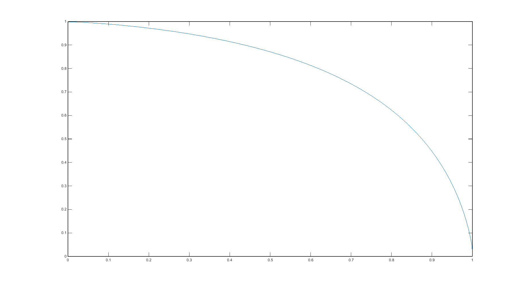
Figure 1. A plot of the function $g$ for the case $p=2$.

Next, for $T=1$ and $x=c=0$ we simulate a path of the optimal control $u\in U(1,0,0)$ and the corresponding strategy $X^{0,u}_{t}=\int_{0}^{t}u_{s}ds$, $t\in[0,1]$. This is done by simulating a Brownian path and applying Theorem 1.3 (see Figures 2-3 below).

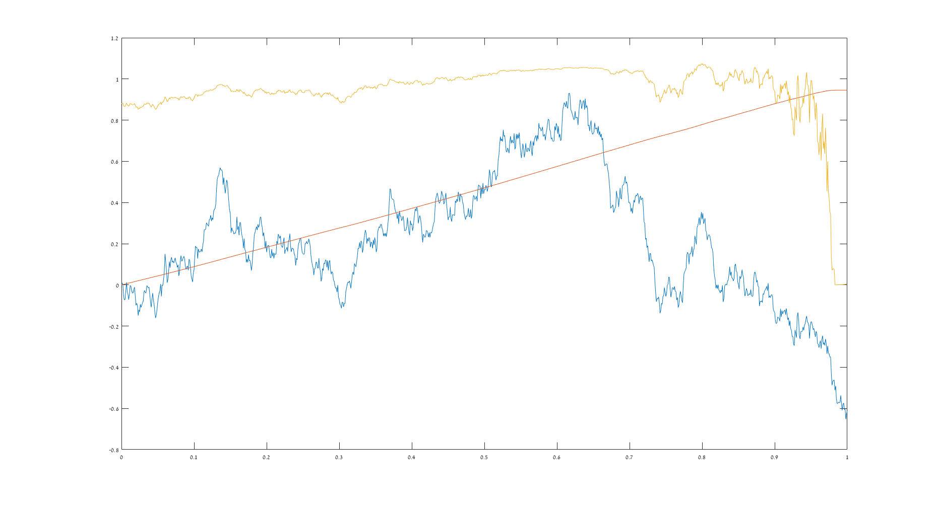
Figure 2. This simulation corresponds to the case where $W_{1}<0$. The Brownian path is in blue, the optimal control $u\in U(1,0,0)$ is in orange and $X^{0,u}_{t}=\int_{0}^{t}u_{s}ds$ is in red.

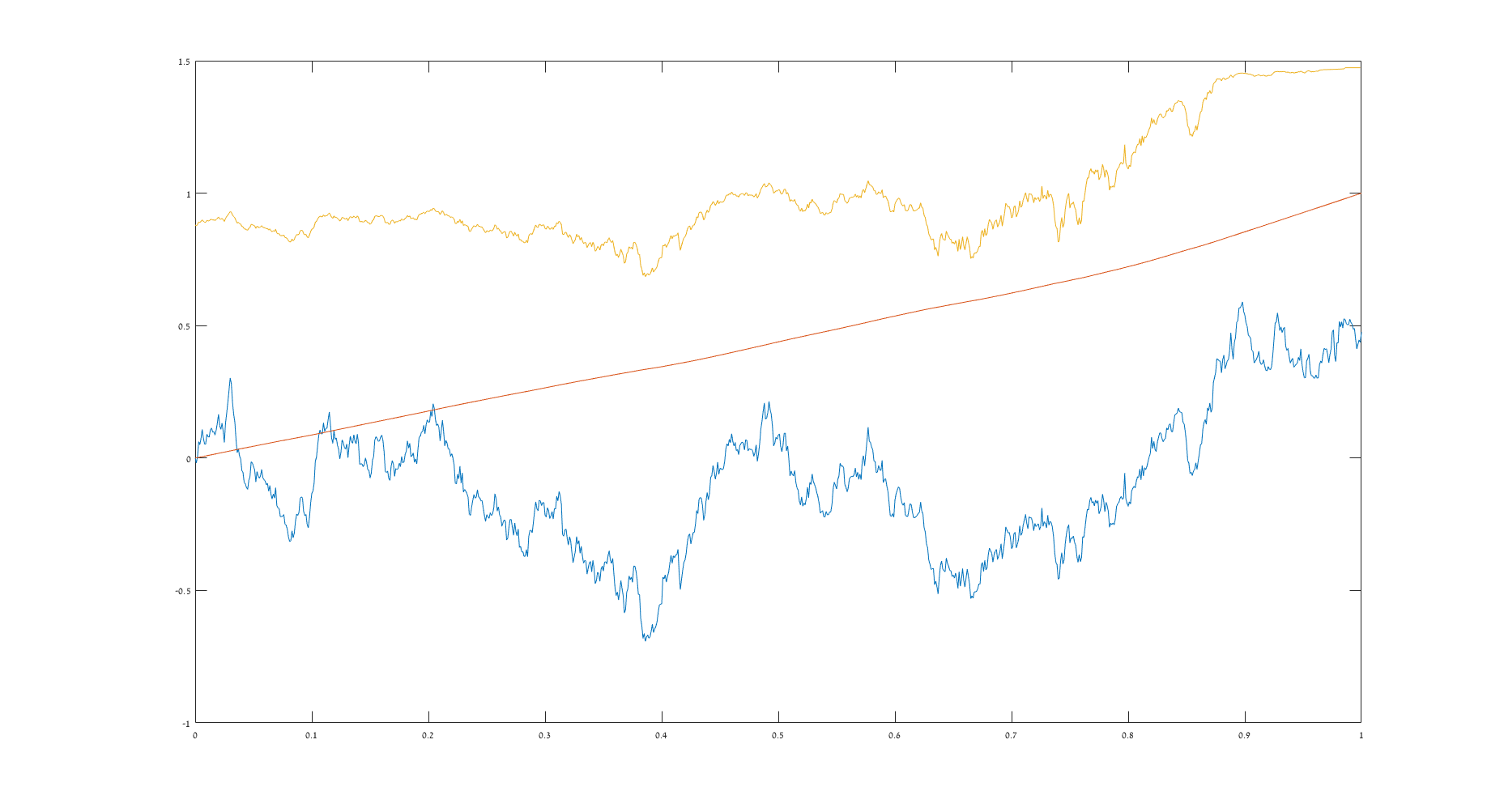
Figure 3. This simulation corresponds to the case where $W_{1}>0$. The Brownian path is in blue, the optimal control $u\in U(1,0,0)$ is in orange and $X^{0,u}_{t}=\int_{0}^{t}u_{s}ds$ is in red.

References

- [1] S. Ankirchner, A. Fromm, T. Kruse and A. Popier, Optimal position targeting via decoupling fields, to appear in Annals of Applied Probability, (2019).
- [2] S. Ankirchner, M. Jeanblanc, and T. Kruse, BSDEs with singular terminal condition and a control problem with constraints, SIAM J. Control Optim., 52, 893–913, (2014).
- [3] S. Ankirchner and T. Kruse, Optimal position targeting with stochastic linear–quadratic costs, Banach Center Publications, 104, 9–24, (2015).
- [4] P. Bank, H.M. Soner, and M. Voss, Hedging with Temporary Price Impact, Mathematics and Financial Economics, 11, 215–239, (2017).
- [5] P. Bank and M. Voss, Linear quadratic stochastic control problems with singular stochastic terminal constraint, SIAM J. Control Optim., 56, 672–699, (2018).
- [6] P. Graewe, U. Horst, and J. Qiu, A non-Markovian liquidation problem and backward SPDEs with singular terminal conditions, SIAM J. Control Optim., 53, 690–711, (2015).
- [7] P. Graewe, U. Horst, and E. Séré, Smooth solutions to portfolio liquidation problems under price-sensitive market impact, Stochastic Processes and their Applications, 128, 976–1006, (2018).
- [8] T. Kruse and A. Popier, Minimal supersolutions for BSDEs with singular terminal condition and application to optimal position targeting, Stochastic Processes and their Applications, 126, 2554 –2592, (2016).
- [9] A. Popier, Backward stochastic differential equations with singular terminal condition, Stochastic Processes and their Applications, 116, 2014–2056, (2006).
- [10] A. Schied, A control problem with fuel constraint and Dawson–Watanabe superprocesses, Ann. Appl. Probab., 23, 2472–2499, (2013).